Workspace Partitioning and Topology Discovery Algorithms for Heterogeneous Multi-Agent Networks

Abstract

In this paper, we consider a class of workspace partitioning problems that arise in the context of area coverage and spatial load balancing for spatially distributed heterogeneous multi-agent networks. It is assumed that each agent has certain directions of motion or directions for sensing and exploration that are more preferable than others. These preferences are measured by means of convex and anisotropic (direction-dependent) quadratic proximity metrics which are, in general, different for each agent. These proximity metrics induce Voronoi-like partitions of the network’s workspace that are comprised of cells which may not always be convex (or even connected) sets but are necessarily contained in ellipsoids that are known to their corresponding agents. The main contributions of this work are 1) a distributed algorithm for the computation of a Voronoi-like partition of the workspace of a heterogeneous multi-agent network and 2) a systematic process to discover the network topology induced by the latter Voronoi-like partition. Numerical simulations that illustrate the efficacy of the proposed algorithms are also presented.

I Introduction

Area coverage and spatial load balancing correspond to two fundamental classes of problems for spatially distributed multi-agent networks. Such problems are typically addressed by means of distributed control algorithms that rely on the use of Voronoi or Voronoi-like (also known as generalized Voronoi) partitions of the workspace of the multi-agent network. For the distributed implementation of these algorithms, each agent has to rely on information encoded in its own cell from the spatial partition and perhaps the cells of its neighbors. However, unless the Voronoi-like partitions are computed by means of distributed partitioning algorithms, the induced control algorithms are not truly distributed. Therefore, the development of distributed partitioning algorithms constitutes an integral component of any Voronoi-distributed control architecture for a multi-agent network. A partitioning algorithm can be characterized as distributed when each agent can compute its own cell independently from its teammates without utilizing a global reference frame while relying on exchange of information with only a subset of them (e.g., those that lie within its communication or sensing range). Ideally, an agent can compute its own cell if it can exchange information with the agents that correspond to its neighbors in the topology of the Voronoi-like partition; these neighboring relations, however, are unknown before the computation of the Voronoi-partition itself. We will refer to the problem of characterizing the set of neighbors (or more realistically, a superset of the latter set) in the topology induced by the Voronoi-like partition as the “network topology discovery problem.”

In this work, we propose distributed algorithms that 1) compute Voronoi-like partitions of the workspace of spatially distributed heterogeneous multi-agent networks and 2) discover the network topology induced by the latter partitions. In our approach, the agents are allowed to have different preferences (hence the qualifier “heterogeneous”) which are measured in terms of relevant proximity (generalized) metrics such as the sensing cost that an agent will incur to obtain measurements from an arbitrary point in its spatial domain or the transition cost (e.g., fuel or battery / energy consumption) that will have to incur to reach it. In our approach, we assume that the proximity metric associated with an agent can be expressed as the sum of a convex quadratic form associated with a positive definite matrix, which we refer to as distance operator [1], and a constant term, which we refer to as additive gain. The distance operators are not necessarily the same for all the agents given that their workspace may exhibit anisotropic features (e.g., certain directions of motion or exploration/sensing are more preferable than others). Some characteristic examples of anisotropic workspaces are oceanic environments, atmospheric domains and hilly terrains in which anisotropic features are induced by ocean currents, winds and elevation variance, respectively. Typically, such anisotropic features are spatially varying and thus it is natural to associate each agent with a different distance operator. We will refer to the Voronoi-like partition of the workspace of a multi-agent network whose agents utilize proximity metrics with different distance operators as the Heterogeneous Quadratic Voronoi Partition (HQVP). In general, the cells that comprise the HQVP may not be convex, or even connected, sets. Consequently, the computation of HQVP and the discovery of the induced network topology is not a straightforward task in sharp contrast with standard Voronoi partitions or other classes of well studied Voronoi-like partitions (e.g., power diagrams).

Literature review: Area coverage and spatial load balancing problems for multi-agent networks have received significant attention in the relevant literature. A well received approach which leverages the so-called Lloyd’s algorithm [2] together with sequences of standard Voronoi partitions can be found in [3]. Several extensions of [3] have appeared in the relevant literature (see, for instance, [4, 5, 6, 7, 8, 9, 10, 11, 12, 13, 14, 15]). The aforementioned papers deal with multi-agent networks that are homogeneous in the sense that all of their agents employ the same proximity metric modulo, perhaps, a different constant term (additive gain). In this work, a multi-agent network will not be classified as heterogeneous unless at least two of its agents have different distance operators and regardless if their additive gains are the same or not. Coverage problems for heterogeneous networks with different distance operators are considered in [16] based on, however, centralized techniques. Finally, the problem of discovering the neighbors of an agent in the topology induced by a standard Voronoi partition has been studied in [17, 18]. The applicability of the methods proposed in these references is limited to standard Voronoi partitions and cannot be extended to the class of spatial partitions considered in this paper.

In our previous work, we have addressed workspace partitioning problems for area coverage by homogeneous multi-agent networks based on proximity (generalized) metrics corresponding to the optimal cost-to-go functions of relevant optimal control problems [19, 20, 21]. In the special case of linear quadratic optimal control problems, the latter metrics correspond to convex quadratic functions whose associated distance operators are, however, the same for all them. Under this strong assumption, the induced Voronoi-like partitions admit a special structure that renders them amenable to computation by means of simple decentralized or distributed algorithms [22, 23, 24]. The problem of inferring the neighbors of an agent in the topology induced by these class of spatial partitions is studied in [24, 21].

Statement of contributions: The main contribution of this work is two-fold. First, we show that under some mild technical assumptions, each cell of the proposed Voronoi-like partition is necessarily contained inside an ellipsoid that is known a priori to its corresponding agent. Next, we present an algorithm which, by leveraging the latter key geometric property, allows each agent to independently compute its own cell from the HQVP. The proposed partitioning algorithm executes a certain number of line searches that seek for the boundary points of the cell of an agent. In contrast with the algorithms proposed in our previous work [25, 26, 24, 21], whose applicability is limited to partitions comprised of convex or star convex cells, the algorithms proposed herein can successfully characterize the cells of a HQVP despite the fact that the latter may be non-convex or even disconnected sets. The proposed algorithms rely on relative position measurements only and thus, neither a global reference frame nor a common grid are required, which is in contrast with most computational geometric techniques for non-standard Voronoi-like partitions [27]. More importantly, the proposed partitioning algorithm can be executed in a distributed way (based on local information) when combined with a network topology discovery algorithm. The main idea of the latter algorithm is to have each agent adjust its communication range so that it can communicate directly (point-to-point communication) with a group of agents from the same network which is a superset of its set of neighbors in the topology of the HQVP without having computed the latter partition.

Structure of the paper: The problem formulation and corresponding preliminaries are presented in Section II. In Section III, we analyze the partitioning problem and present certain key properties enjoyed by its solution. The distributed partitioning algorithm is presented in Section IV whereas the network topology discovery problem is analyzed and solved in Section V. Section VI presents numerical simulations, and finally, Section VII concludes the paper with a summary of remarks together with directions for future work.

II Preliminaries and Problem Formulation

II-A Notation

We denote by $\mathbb{R}^{n}$ the set of $n$-dimensional real vectors and by $\mathbb{R}_{\geq 0}$ the set of non-negative real numbers. We write $\mathbb{Z}$ to denote the set of integers. Given $\tau_{1}$, $\tau_{2}\in\mathbb{Z}$ with $\tau_{1}\leq\tau_{2}$, we define the discrete interval from $\tau_{1}$ to $\tau_{2}$ as follows: $[\tau_{1},\tau_{2}]_{\mathbb{Z}}=[\tau_{1},\tau_{2}]\cap\mathbb{Z}$. We write $|\alpha|$ to denote the 2-norm of a vector $\alpha\in\mathbb{R}^{n}$. Moreover, we write $\mathbf{A}\succ\mathbf{0}$ to denote that a symmetric matrix $\mathbf{A}=\mathbf{A}^{\mbox{\scriptsize T}}$ is positive definite. Given $\mathbf{A}=\mathbf{A}^{\mbox{\scriptsize T}}$, $\mathbf{B}=\mathbf{B}^{\mbox{\scriptsize T}}$, we write $\mathbf{A}\succ\mathbf{B}$ if and only if $\mathbf{A}-\mathbf{B}\succ\mathbf{0}$. Furthermore, given a symmetric matrix $\mathbf{P}=\mathbf{P}^{\mbox{\scriptsize T}}$, we denote by $\lambda_{\min}(\mathbf{P})$ and $\lambda_{\max}(\mathbf{P})$ its minimum and maximum (real) eigenvalues, respectively. Given $x\in\mathbb{R}^{n}$, $\mathbf{\Sigma}\succ\mathbf{0}$, and $\gamma>0$, we write $\mathcal{E}_{\gamma}(x;\mathbf{\Sigma}^{-1})$ to denote the ellipsoid $\{z\in\mathbb{R}^{n}:(z-x)^{\mbox{\scriptsize T}}\mathbf{\Sigma}(z-x)\leq\gamma\}$. We denote by $\mathcal{B}_{\rho}(x_{c})$ the closed ball of radius $\rho>0$ centered at $x_{c}$, that is, $\mathcal{B}_{\rho}(x_{c}):=\{z\in\mathbb{R}^{n}:|z-x_{c}|\leq\rho\}$. Furthermore, $\mathrm{bd}(\mathcal{A})$ and $\mathrm{rbd}(\mathcal{A})$ denote the boundary and the relative boundary of a set $\mathcal{A}$, whereas $\operatorname{int}(\mathcal{A})$ and $\mathrm{rint}(\mathcal{A})$ denote its interior and relative interior. The powerset of a set $\mathcal{A}$ is denoted as $\wp(\mathcal{A})$. Given $\mathcal{A}$, $\mathcal{B}\subseteq\mathbb{R}^{n}$, we denote by $\mathcal{A}\oplus\mathcal{B}$ their Minkowski sum, that is, $\mathcal{A}\oplus\mathcal{B}:=\{x=y+z:y\in\mathcal{A}~{}\text{and}~{}z\in\mathcal{B}\}$, and by $\mathcal{A}\ominus\mathcal{B}$ their Minkowski difference, that is, $\mathcal{A}\ominus\mathcal{B}:=\{x:\{x\}\oplus\mathcal{B}\subseteq\mathcal{A}\}$. Given $\alpha$, $\beta\in\mathbb{R}^{n}$, we denote by $[\alpha,\beta]$ the line segment connecting them (including the two endpoints), that is, $[\alpha,\beta]:=\{{x}\in\mathbb{R}^{n}:~{}{x}=t\alpha+(1-t)\beta,~{}t\in[0,1]\}$. In addition, we denote by $]\alpha,\beta]$ and $[\alpha,\beta[$ the sets $[\alpha,\beta]\backslash\{\alpha\}$ and $[\alpha,\beta]\backslash\{\beta\}$, respectively.

II-B The Partitioning Problem for a Heterogeneous Multi-Agent Network

In this section, we formulate the partitioning problem for a multi-agent network comprised of $n$ agents distributed over a spatial domain $\mathcal{S}$, which is assumed to be a convex and compact set. To the latter network we attach an additional agent, which we refer to as the $0$-th agent of the network. The latter agent may correspond, for instance, to a vehicle station from which vehicles are dispatched in response to requests issued in the vicinity of the station or a “mother vehicle” that can deploy $n$ mobile sensors to collect measurements from various nearby locations. We will refer to the network that includes the $0$-th agent as the extended network. It is assumed that the agents are located at $n+1$ distinct locations in $\mathcal{S}$, which form the point-set $X:=\{x_{i}\in\mathcal{S}:~{}i\in[0,n]_{\bm{\mathbb{Z}}}\}$.

Our first objective is to subdivide $\mathcal{S}$ into $n+1$ non-overlapping subsets that will be associated with the $n+1$ agents of the extended network in an one-to-one way. We will refer to these subsets of $\mathcal{S}$ as regions of influence (ROI) or simply cells that comprise a spatial partition of the network’s workspace. In particular, the interior of each cell will consist exclusively of points in $\mathcal{S}$ that are “closer” to its corresponding agent than to any other agent of the extended network. The closeness between the $i$-th agent and an arbitrary point $x\in\mathcal{S}$ will be measured in terms of an appropriate convex quadratic proximity (generalized) metric $\delta(\cdot;x_{i}):\mathcal{S}\rightarrow\mathbb{R}_{\geq 0}$ with

$$\delta_{i}(x;x_{i}):=(x-x_{i})^{\mbox{\scriptsize T}}\mathbf{P}_{i}(x-x_{i})+\mu_{i},$$ (1)

where $\mu_{i}\geq 0$ and $\mathbf{P}_{i}\succ\mathbf{0}$ for all $i\in[0,n]_{\mathbb{Z}}$. We will refer to $\mu_{i}$ and $\mathbf{P}_{i}$ as the $i$-th additive gain and distance operator, respectively. The proximity metric $\delta_{i}(x;x_{i})$ corresponds, for instance, to the cost that the $i$-th agent will incur for its transition from point $x_{i}$ to point $x$. Alternatively, it may reflect the sensing cost that the $i$-th agent, which is located at $x_{i}$, will incur in order to obtain measurements from point $x$. In particular, let us consider the bivariate Gaussian distribution with mean $m_{i}\in\mathbb{R}^{2}$ and covariance $\mathbf{\Sigma}_{i}\succ\mathbf{0}$ whose probability density function is given by

$$\rho_{i}(x):=\big{(}2\pi\sqrt{\det(\mathbf{\Sigma}_{i})}\big{)}^{-1}\mathrm{exp}\big{(}-\tfrac{1}{2}(x-m_{i})^{\mbox{\scriptsize T}}\mathbf{\Sigma}^{-1}_{i}(x-m_{i})\big{)}$$

and let us define the sensing cost as follows [28]:

$$c_{i}(x) :=-\mathrm{log}(\rho_{i}(x))$$

$$=\log\big{(}2\pi\sqrt{\det(\mathbf{\Sigma}_{i})}\big{)}+\tfrac{1}{2}(x-m_{i})^{\mbox{\scriptsize T}}\mathbf{\Sigma}^{-1}_{i}(x-m_{i}).$$

Therefore, by taking $\mathbf{P}_{i}:=\tfrac{1}{2}\mathbf{\Sigma}^{-1}_{i}$, $x_{i}=m_{i}$ and $\mu_{i}:=\log(2\pi\sqrt{\det(\mathbf{\Sigma}_{i})}$, we have $\delta_{i}(x;x_{i})=c_{i}(x)$.

It is worth noting that the $i$-th additive gain $\mu_{i}$ corresponds to the minimum value of $\delta_{i}(x;x_{i})$, which is attained at $x=x_{i}$, that is, $\mu_{i}=\min_{x\in\mathcal{S}}\delta_{i}(x;x_{i})=\delta_{i}(x_{i};x_{i})$. In addition, the $i$-th distance operator $\mathbf{P}_{i}$ determines which directions, if any, are more preferable to the $i$-th agent than others. In particular, if $\mathbf{P}_{i}=\lambda_{i}\mathbf{I}$, where $\lambda_{i}>0$, then the level sets of the quadratic form $(x-x_{i})^{\mbox{\scriptsize T}}\mathbf{P}_{i}(x-x_{i})$ are circles and thus there are no preferable directions; otherwise, the latter level sets become ellipses whose major axes determine the most preferable directions. In the first case, $\mathbf{P}_{i}$ is an isotropic distance operator (i.e., direction independent), whereas in the second, and more interesting case, is an anisotropic (i.e., direction-dependent) distance operator. It is worth noting that requiring the existence of a matrix $\overline{\mathbf{P}}\succ\mathbf{0}$ such that $\mathbf{P}_{i}=\overline{\mathbf{P}}$ for all $i\in[0,n]_{\mathbb{Z}}$ can be a very restrictive assumption in practice. In this work, we will consider the more general case in which there always exists $(i,j)$ with $i\neq j$ such that $\mathbf{P}_{i}\neq\mathbf{P}_{j}$ and we will refer to the multi-agent network as “heterogeneous.”

Next, we provide a number of technical, yet practically intuitive, assumptions that will help us streamline the subsequent discussion and analysis.

Assumption 1

For any $i\in[0,n]_{\mathbb{Z}}$, we have that $\delta_{i}(x_{i};x_{i})<\delta_{j}(x_{i};x_{j})$ or, equivalently,

$$(x_{j}-x_{i})^{\mbox{\scriptsize T}}\mathbf{P}_{j}(x_{j}-x_{i})+\mu_{j}>\mu_{i},$$ (2)

for all $j\neq i$, provided that $x_{i}\neq x_{j}$.

The previous assumption implies that the distance of the $j$-th agent from the location $x_{i}$ of the $i$-th agent, which is equal to $\delta_{j}(x_{i};x_{j})$, has to be greater than the distance of the $i$-th agent from itself, which is equal to $\delta_{i}(x_{i};x_{i})=\mu_{i}$. For instance, in the case of a sensor network, condition (2) implies that no sensor different from the $i$-th sensor can obtain more accurate measurements from the location $x_{i}$ of the $i$-th agent.

• Although Assumption 1 is quite intuitive, one may argue that there may exist applications in which it may not hold true. It should be mentioned here that the partitioning algorithm that will be presented herein can be applied even when Assumption 1 is removed, after the necessary modifications have been carried out (we will comment on some of these modifications later on). Assumption 1 will allow us to streamline the presentation and avoid discussing special cases of low interest.

Assumption 2

We assume that

$$\mathbf{P}_{i}\succ\mathbf{P}_{0}\succ\mathbf{0},~{}~{}~{}~{}\mu_{i}\geq\mu_{0}\geq 0,~{}~{}~{}~{}\forall i\in[1,n]_{\bm{\mathbb{Z}}}.$$ (3)

The following proposition will allow us to better understand the implications of Assumption 2.

Proposition 1

Let $\gamma>\max_{i\in[1,n]_{\bm{\mathbb{Z}}}}\mu_{i}$ and let $\mathsf{x}\in\mathcal{S}$. In addition, let $\mathcal{D}^{0}_{\gamma}(\mathsf{x})$ and $\mathcal{D}^{i}_{\gamma}(\mathsf{x})$ denote the $\gamma$- sublevel-sets of, respectively, $\delta_{0}(\cdot;x_{0})$ and $\delta_{i}(\cdot;x_{i})$ when $x_{i}\equiv x_{0}\equiv\mathsf{x}$ for all $i\in[1,n]_{\bm{\mathbb{Z}}}$, that is, $\mathcal{D}_{\gamma}^{0}(\mathsf{x}):=\{x\in\mathcal{S}:~{}\delta_{0}(x;\mathsf{x})\leq\gamma\}$ and $\mathcal{D}_{\gamma}^{i}(\mathsf{x}):=\{x\in\mathcal{S}:~{}\delta_{i}(x;\mathsf{x})\leq\gamma\}$, for $i\in[1,n]_{\bm{\mathbb{Z}}}$. Then, the following set inclusion holds:

$$\mathcal{D}_{\gamma}^{i}(\mathsf{x})\subsetneq\mathcal{D}_{\gamma}^{0}(\mathsf{x}),~{}~{}~{}\forall i\in[1,n]_{\bm{\mathbb{Z}}}.$$ (4)

Proof:

In view of (1), $\mathcal{D}_{\gamma}^{0}(\mathsf{x})$ and $\mathcal{D}_{\gamma}^{i}(\mathsf{x})$ can be expressed as follows:

$$\mathcal{D}_{\gamma}^{0}(\mathsf{x}) =\{x\in\mathcal{S}:~{}(x-\mathsf{x})^{\mbox{\scriptsize T}}\mathbf{P}_{0}(x-\mathsf{x})\leq\gamma-\mu_{0}\},$$

$$\mathcal{D}_{\gamma}^{i}(\mathsf{x}) =\{x\in\mathcal{S}:~{}(x-\mathsf{x})^{\mbox{\scriptsize T}}\mathbf{P}_{i}(x-\mathsf{x})\leq\gamma-\mu_{i}\}.$$

By hypothesis $\gamma>\mu_{i}\geq\mu_{0}\geq 0$, and thus

$$\mathcal{D}_{\gamma}^{0}(\mathsf{x}) \supseteq\{x\in\mathcal{S}:~{}(x-\mathsf{x})^{\mbox{\scriptsize T}}\mathbf{P}_{0}(x-\mathsf{x})\leq\gamma-\mu_{i}\}$$

$$\supsetneq\{x\in\mathcal{S}:~{}(x-\mathsf{x})^{\mbox{\scriptsize T}}\mathbf{P}_{i}(x-\mathsf{x})\leq\gamma-\mu_{i}\}$$

$$=\mathcal{D}_{\gamma}^{i}(\mathsf{x}),$$

where the second set inclusion follows from the fact that $\mathbf{P}_{i}\succ\mathbf{P}_{0}\succ\mathbf{0}$. Thus, the set inclusion (4) holds true. ∎

• It is worth noting that $\mathcal{D}_{\gamma}^{0}(\mathsf{x})=\mathcal{E}_{\gamma-\mu_{0}}(\mathsf{x};\mathbf{P}_{0}^{-1})\cap\mathcal{S}$ and $\mathcal{D}_{\gamma}^{i}(\mathsf{x})=\mathcal{E}_{\gamma-\mu_{i}}(\mathsf{x};\mathbf{P}_{i}^{-1})\cap\mathcal{S}$. Proposition 1 implies that the footprint of the set of points that are within distance $\gamma$ from the $0$-th agent (distance measured in terms of $\delta_{0}$) is greater than the footprint of the set of points that are within distance $\gamma$ from the $i$-th agent (distance measured now in terms of $\delta_{i}$) when both of the agents are placed at an arbitrary common point $\mathsf{x}\in\mathcal{S}$.

II-C Formulation of the Workspace Partitioning Problem

We can now give the precise definitions of the Voronoi-like partition of $\mathcal{S}$ generated by the extended multi-agent network based on the quadratic proximity metrics defined in (1).

Definition 1

Suppose that $\mathcal{S}\in\mathbb{R}^{2}$ is a compact and convex set and let $X\subset\mathcal{S}$ be a set comprised of $n+1$ distinct points (locations of the agents). Then, we say that the collection of sets $\mathcal{V}(X;\mathcal{S}):=\{\mathcal{V}^{i}\in\wp(\mathcal{S}):~{}i\in[0,n]_{\bm{\mathbb{Z}}}\}$ where

$$\mathcal{V}^{i}:=\{x\in\mathcal{S}:~{}\delta_{i}(x;x_{i})\leq\min_{j\neq i}\delta_{j}(x;x_{j})\},$$ (5)

forms a Heterogeneous Quadratic Voronoi Partition (HQVP) of $\mathcal{S}$ that is generated by $X$. In particular, $\mathrm{i})$ $\mathcal{S}=\cup_{i\in[0,n]_{\mathbb{Z}}}\mathcal{V}^{i}$ and $\mathrm{ii})$ $\operatorname{int}(\mathcal{V}^{i})\cap\operatorname{int}(\mathcal{V}^{j})=\varnothing$, for $i\neq j$. We will refer to the set $\mathcal{V}^{i}$ as the $i$-th cell or region-of-influence (ROI).

The following proposition highlights some fundamental properties of the HQVP.

Proposition 2

Let $\mathcal{V}^{i}\in\mathcal{V}(X;\mathcal{S})$. Then, $\delta_{i}(x;x_{i})\leq\min_{j\neq i}\delta_{j}(x;x_{j})$ for all $x\in\mathcal{V}^{i}$ and in particular,

1. $\delta_{i}(x;x_{i})<\min_{j\neq i}\delta_{j}(x;x_{j}),~{}~{}\forall x\in\operatorname{int}(\mathcal{V}^{i})$

2. $\delta_{i}(x;x_{i})=\min_{j\neq i}\delta_{j}(x;x_{j}),~{}~{}\forall x\in\mathrm{bd}(\mathcal{V}^{i})\backslash\mathrm{bd}(\mathcal{S})$, that is, there exists $j=j_{x}$ such that $\delta_{i}(x;x_{i})=\delta_{j_{x}}(x;x_{j_{x}})$.

It is worth considering what would happen if we dropped Assumption 2 and assumed instead that $\mu_{i}=\bar{\mu}$ and $\mathbf{P}_{i}=\lambda\mathbf{I}$, for all $i\in[0,n]_{\bm{\mathbb{Z}}}$, where $\bar{\mu}\geq 0$ and $\lambda>0$. In this special case, each agent employs the same proximity metric; in particular, $\delta_{i}(x;x_{i})=\lambda|x-x_{i}|^{2}+\bar{\mu}$, for all $i\in[0,n]_{\bm{\mathbb{Z}}}$. In this case,

$$\mathcal{V}^{i} :=\{x\in\mathcal{S}:~{}\lambda|x-x_{i}|^{2}\leq\lambda\min_{j\in[0,n]_{\bm{\mathbb{Z}}}}|x-x_{j}|^{2}\}$$

$$=\{x\in\mathcal{S}:~{}|x-x_{i}|\leq\min_{j\in[0,n]_{\bm{\mathbb{Z}}}}|x-x_{j}|\},$$

which is precisely the definition of the $i$-th cell of the standard Voronoi partition [29]. Consequently, in this special case, the HQVP reduces to the standard Voronoi partition which has combinatorial complexity in $\mathcal{O}(n)$ and computational complexity in $\mathcal{O}(n\log(n))$. Another special case while keeping Assumption 2 inactive, is when there is a pair $(i,j)$, with $i\neq j$, such that $\mu_{i}\neq\mu_{j}$ and $\mathbf{P}_{i}=\overline{\mathbf{P}}$, for all $i\in[0,n]_{\bm{\mathbb{Z}}}$, where $\overline{\mathbf{P}}\succ\mathbf{0}$. As we have shown in [22], the HQVP in the latter case reduces to an affine diagram, which has combinatorial complexity in $\Theta(n)$ and computational complexity in $\Theta(n\log n+n)$ [30] (note that the latter complexities are modest and close to those of the standard Voronoi partition). In this work, in view of Assumption 2, there always exists a pair $(i,j)$, with $i\neq j$, such that $\mathbf{P}_{i}\neq\mathbf{P}_{j}$ (one can take $j=0$ and any $i\in[1,n]_{\bm{\mathbb{Z}}}$). According to [31], the HQVP has combinatorial complexity $\Theta(n^{3})$ and computational complexity in $\mathcal{O}(n^{3}+n\log(n))$; these complexities are significantly higher than those of the standard and the affine Voronoi partitions. One important fact is that the cells of HQVP are not necessarily convex sets (they may even be disconnected sets), which makes their computation by means of distributed algorithms quite challenging. By virtue of the previous discussion, it should become clear that the partitioning algorithms proposed in our previous work [25, 26, 24, 21], which can only compute affine partitions or partitions comprised of star convex cells for homogeneous multi-agent networks, are not applicable to the partitioning problem for heterogeneous networks which is considered herein. The latter problem requires the development of new and more powerful tools which are applicable to partitions comprised of cells which can be non-convex or even disconnected sets.

Next, we formulate the uncoupled partitioning problem in which the $i$-th agent of the network is required to compute its own cell in HQVP independently from its teammates.

Problem 1

Uncoupled Partitioning Problem over $\mathcal{S}$: Let $\mathcal{V}(X;\mathcal{S})=\{\mathcal{V}_{i}\in\wp(\mathcal{S}):~{}i\in[0,n]_{\bm{\mathbb{Z}}}\}$ be the HQVP of $\mathcal{S}$ generated by the point-set $X:=\{x_{i}\in\mathcal{S}:~{}i\in[0,n]_{\bm{\mathbb{Z}}}\}$. For a given $i\in[1,n]_{\bm{\mathbb{Z}}}$, compute the cell $\mathcal{V}^{i}\in\mathcal{V}(X;\mathcal{S})$, independently from the other cells of the same partition.

• It is worth noting that the computation of the cell $\mathcal{V}^{0}$ which is assigned to the $0$-th agent of the extended network is not included in the formulation of Problem 1. The latter set corresponds to the part of the spatial domain $\mathcal{S}$ that is not claimed by any agent of the actual network or in other words, the coverage hole of the latter network, that is, $\mathcal{V}^{0}=\mathcal{S}\backslash\big{(}\cup_{i=1}^{n}\mathcal{V}^{i}\big{)}$. Intuitively, this means that at any point in $\mathcal{V}^{0}$, the ground station or mother vehicle (the latter correspond to interpretations of the hypothetical $0$-th agent) can rely to their own sensing capabilities and therefore, they do not have to dispatch any mobile sensors from the actual network to take in-situ measurements there. Note that the non-emptiness of the coverage hole $\mathcal{V}^{0}$ is a direct consequence of Assumption 2.

II-D Formulation of the Network Topology Discovery Problem

In a nutshell, the goal of the network topology discovery problem is to find a systematic way that will allow the $i$-th agent of the network to determine its neighbors in the topology induced by the HQVP.

Definition 2

The $i$-th agent and the $j$-th agent, which are located at $x_{i}\in X$ and $x_{j}\in X$, respectively, are neighbors in the topology of $\mathcal{V}(X;\mathcal{S})$, if the boundaries of their cells have a non-empty intersection, that is, $\mathrm{bd}(\mathcal{V}^{i})\cap\mathrm{bd}(\mathcal{V}^{j})\neq\varnothing$.

Now, let us denote by $\mathcal{N}_{i}$ the index set of the neighbors of the $i$-th agent. In view of Definition 2,

$$\mathcal{N}_{i}:=\{\ell\in[0,n]_{\bm{\mathbb{Z}}}\backslash\{i\}:\mathrm{bd}(\mathcal{V}^{\ell})\cap\mathrm{bd}(\mathcal{V}^{i})\neq\varnothing\}.$$ (6)

Proposition 3

The index-set of the neighbors of the $i$-th agent, $\mathcal{N}_{i}$, consists of all $\ell\in[0,n]_{\bm{\mathbb{Z}}}\backslash\{i\}$ such that $\delta_{\ell}(x;x_{\ell})=\delta_{i}(x;x_{i})$ for some $x\in\mathrm{bd}(\mathcal{V}^{i})\backslash\mathrm{bd}(\mathcal{S})$.

Proof:

The proof follows readily from Proposition 2. ∎

The network topology discovery problem seeks for a lower bound on the communication range $\eta_{i}$ of the $i$-th agent such that its communication region $\mathcal{B}_{\eta_{i}}(x_{i})$ contains all of its neighbors in the topology of HQVP.

Problem 2

Network Topology Discovery Problem: Find a lower bound $\underline{\eta_{i}}>0$ on the communication range $\eta_{i}$ of the $i$-th agent, for $i\in[1,n]_{\bm{\mathbb{Z}}}$, such that its communication region, $\mathcal{B}_{\eta_{i}}(x_{i})$, contains all of its neighbors, that is,

$$\mathcal{B}_{\eta_{i}}(x_{i})\supsetneq\{x_{k}\in X:~{}k\in\mathcal{N}_{i}\},~{}~{}\forall\eta_{i}\geq\underline{\eta_{i}}.$$ (7)

III Analysis and Solution of the Uncoupled Partitioning Problem

III-A Analysis of the Uncoupled Partitioning Problem

In this section, we will present some useful properties enjoyed by the cells comprising the HQVP which we will subsequently leverage to develop distributed algorithms for the computation of the solution to Problem 1. The first step of our analysis will be the characterization of the bisector, $\mathfrak{B}_{i,j}$, that corresponds to the loci of all points in $\mathcal{S}$ that are equidistant from the $i$-th and the $j$-th agents with $i\neq j$, that is,

$$\mathfrak{B}_{i,j}:=\{x\in\mathcal{S}:~{}\delta_{i}(x;x_{i})=\delta_{j}(x;x_{j})\}.$$ (8)

The equation $\delta_{i}(x;x_{i})=\delta_{j}(x;x_{j})$ is equivalent to

$$(x-x_{i})^{\mbox{\scriptsize T}}\mathbf{P}_{i}(x-x_{i})+\mu_{i}=(x-x_{j})^{\mbox{\scriptsize T}}\mathbf{P}_{j}(x-x_{j})+\mu_{j}$$

which can be written more compactly as follows

$$x^{\mbox{\scriptsize T}}\mathbf{P}_{i,j}x-2\chi_{i,j}^{\mbox{\scriptsize T}}x+\sigma_{i,j}=0,$$ (9)

where

$$\mathbf{P}_{i,j} :=\mathbf{P}_{i}-\mathbf{P}_{j},$$ (10a)

$$\chi_{i,j} :=\mathbf{P}_{i}x_{i}-\mathbf{P}_{j}x_{j},$$ (10b)

$$\sigma_{i,j} :=|\mathbf{P}_{i}^{1/2}x_{i}|^{2}+\mu_{i}-|\mathbf{P}^{1/2}_{j}x_{j}|^{2}-\mu_{j}.$$ (10c)

If $\mathbf{P}_{i,j}=\mathbf{0}$, that is, $\mathbf{P}_{i}=\mathbf{P}_{j}$, equation (9) describes a straight line. In the more interesting case when $\mathbf{P}_{i,j}\neq\mathbf{0}$, (9) corresponds to a quadratic vector equation that determines a conic section.

Next, we will leverage Assumption 2 to show that the cell $\mathcal{V}^{i}$, for $i\in[1,n]_{\bm{\mathbb{Z}}}$, enjoys an important property that will prove very useful in our subsequent analysis. To this aim, we first note that, in view of Assumption 2, $\mathbf{P}_{i}\succ\mathbf{P}_{0}$ or equivalently $\mathbf{P}_{i,0}\succ\mathbf{0}$. Next, by completing the square in (9) and then setting $j=0$, we get

$$0 =x^{\mbox{\scriptsize T}}\mathbf{P}_{i,0}x-2\chi_{i,0}^{\mbox{\scriptsize T}}\mathbf{P}_{i,0}^{-1/2}\mathbf{P}_{i,0}^{1/2}x+\chi_{i,0}^{\mbox{\scriptsize T}}\mathbf{P}_{i,0}^{-1}\chi_{i,0}$$

$$~{}~{}~{}-\chi_{i,0}^{\mbox{\scriptsize T}}\mathbf{P}_{i,0}^{-1}\chi_{i,0}+\sigma_{i,0}$$

from which it follows that

$$|\mathbf{P}_{i,0}^{1/2}(x-\mathbf{P}_{i,0}^{-1}\chi_{i,0})|^{2}=|\mathbf{P}_{i,0}^{-1/2}\chi_{i,0}|^{2}-\sigma_{i,0}.$$ (11)

Therefore, the bisector $\mathfrak{B}_{i,0}$ consists of all points $x\in\mathcal{S}$ that satisfy Eq. (11), which is the equation of an ellipse provided that the right hand side of the latter equation is a strictly positive number.

Proposition 4

Let $i\in[1,n]_{\bm{\mathbb{Z}}}$ and let

$$\ell_{i,0}:=|\mathbf{P}_{i,0}^{-1/2}\chi_{i,0}|^{2}-\sigma_{i,0},$$ (12)

where $\mathbf{P}_{i,0}$, $\chi_{i,0}$ and $\sigma_{i,0}$ are as defined in (10a)–(10c) for $j=0$. Then, $\ell_{i,0}>0$ and the bisector $\mathfrak{B}_{i,0}$ satisfies

$$\mathfrak{B}_{i,0}=\mathrm{bd}(E_{i})\cap\mathcal{S},$$ (13)

where $E_{i}:=\mathcal{E}_{\ell_{i,0}}(\mathbf{P}_{i,0}^{-1}\chi_{i,0};\mathbf{P}_{i,0}^{-1})$.

Proof:

In view of (10a)-(10b) for $j=0$, we have

$$|\mathbf{P}_{i,0}^{-1/2}\chi_{i,0}|^{2} =|\mathbf{P}_{i,0}^{-1/2}(\mathbf{P}_{i}x_{i}-\mathbf{P}_{0}x_{0})|^{2}$$

$$=x_{i}^{\mbox{\scriptsize T}}\mathbf{P}_{i}\mathbf{P}_{i,0}^{-1}\mathbf{P}_{i}x_{i}+x_{0}^{\mbox{\scriptsize T}}\mathbf{P}_{0}\mathbf{P}_{i,0}^{-1}\mathbf{P}_{0}x_{0}$$

$$~{}~{}~{}~{}-2x_{i}^{\mbox{\scriptsize T}}\mathbf{P}_{i}\mathbf{P}_{i,0}^{-1}\mathbf{P}_{0}x_{0}$$

$$=[x_{i}^{\mbox{\scriptsize T}},~{}x_{0}^{\mbox{\scriptsize T}}]\begin{bmatrix}\mathbf{P}_{i}\mathbf{P}_{i,0}^{-1}\mathbf{P}_{i}&-\mathbf{P}_{i}\mathbf{P}_{i,0}^{-1}\mathbf{P}_{0}\\ -\mathbf{P}_{0}\mathbf{P}_{i,0}^{-1}\mathbf{P}_{i}&\mathbf{P}_{0}\mathbf{P}_{i,0}^{-1}\mathbf{P}_{0}\end{bmatrix}\begin{bmatrix}x_{i}\\ x_{0}\end{bmatrix}.$$

In addition, from (10c) for $j=0$, we get

$$\sigma_{i,0} =|\mathbf{P}_{i}^{1/2}x_{i}|^{2}+\mu_{i}-|\mathbf{P}^{1/2}_{0}x_{0}|^{2}-\mu_{0}$$

$$=x_{i}^{\mbox{\scriptsize T}}\mathbf{P}_{i}x_{i}-x_{0}^{\mbox{\scriptsize T}}\mathbf{P}_{0}x_{0}+\mu_{i}-\mu_{0}$$

$$=[x_{i}^{\mbox{\scriptsize T}},~{}x_{0}^{\mbox{\scriptsize T}}]\begin{bmatrix}\mathbf{P}_{i}&\mathbf{0}\\ \mathbf{0}&-\mathbf{P}_{0}\end{bmatrix}\begin{bmatrix}x_{i}\\ x_{0}\end{bmatrix}+\mu_{i}-\mu_{0}.$$

Therefore, we have that

$$\ell_{i,0} =|\mathbf{P}_{i,0}^{-1/2}\chi_{i,0}|^{2}-\sigma_{i,0}$$

$$=[x_{i}^{\mbox{\scriptsize T}},~{}x_{0}^{\mbox{\scriptsize T}}]\begin{bmatrix}\mathbf{P}_{i}\mathbf{P}_{i,0}^{-1}\mathbf{P}_{i}-\mathbf{P}_{i}&-\mathbf{P}_{i}\mathbf{P}_{i,0}^{-1}\mathbf{P}_{0}\\ -\mathbf{P}_{0}\mathbf{P}_{i,0}^{-1}\mathbf{P}_{i}&\mathbf{P}_{0}\mathbf{P}_{i,0}^{-1}\mathbf{P}_{0}+\mathbf{P}_{0}\end{bmatrix}\begin{bmatrix}x_{i}\\ x_{0}\end{bmatrix}$$

$$~{}~{}~{}+\mu_{0}-\mu_{i}.$$ (14)

Now, in view of (2) for $j=0$, we have that

$$\mu_{0}-\mu_{i} >-(x_{0}-x_{i})^{\mbox{\scriptsize T}}\mathbf{P}_{0}(x_{0}-x_{i})$$

$$=[x_{i}^{\mbox{\scriptsize T}},~{}~{}x_{0}^{\mbox{\scriptsize T}}]\begin{bmatrix}-\mathbf{P}_{0}&\mathbf{P}_{0}\\ \mathbf{P}_{0}&-\mathbf{P}_{0}\end{bmatrix}\begin{bmatrix}x_{i}\\ x_{0}\end{bmatrix}.$$ (15)

Therefore, in view of (14), (III-A) gives

$$\ell_{i,0}>[x_{i}^{\mbox{\scriptsize T}},~{}x_{0}^{\mbox{\scriptsize T}}]\mathbf{\Psi}\begin{bmatrix}x_{i}\\ x_{0}\end{bmatrix},~{}~{}~{}~{}~{}~{}\mathbf{\Psi}:=\begin{bmatrix}\mathbf{\Psi}_{11}&\mathbf{\Psi}_{12}\\ \mathbf{\Psi}_{12}^{\mbox{\scriptsize T}}&\mathbf{\Psi}_{22}\end{bmatrix},$$ (16)

where $\mathbf{\Psi}_{11},\mathbf{\Psi}_{12}$, $\mathbf{\Psi}_{13}\in\mathbb{R}^{2\times 2}$ are defined as follows:

$$\mathbf{\Psi}_{11} :=\mathbf{P}_{i}\mathbf{P}_{i,0}^{-1}\mathbf{P}_{i}-\mathbf{P}_{i}-\mathbf{P}_{0},$$ (17a)

$$\mathbf{\Psi}_{12} :=-\mathbf{P}_{i}\mathbf{P}_{i,0}^{-1}\mathbf{P}_{0}+\mathbf{P}_{0},$$ (17b)

$$\mathbf{\Psi}_{22} :=\mathbf{P}_{0}\mathbf{P}_{i,0}^{-1}\mathbf{P}_{0}.$$ (17c)

Note that $\mathbf{\Psi}_{22}=\mathbf{P}_{0}\mathbf{P}_{i,0}^{-1}\mathbf{P}_{0}\succ\mathbf{0}$. Next, we show that the Schur complement of the block $\mathbf{\Psi}_{22}$ of the block matrix $\mathbf{\Psi}$, which is denoted as $(\mathbf{\Psi}/\mathbf{\Psi}_{22})$ and defined as $(\mathbf{\Psi}/\mathbf{\Psi}_{22}):=\mathbf{\Psi}_{11}-\mathbf{\Psi}_{12}\mathbf{\Psi}_{22}^{-1}\mathbf{\Psi}_{12}^{\mbox{\scriptsize T}}$, is positive definite, that is, $(\mathbf{\Psi}/\mathbf{\Psi}_{22})\succ\mathbf{0}$. Indeed, in view of (17a)-(17c)

$$(\mathbf{\Psi}/\mathbf{\Psi}_{22}) =\mathbf{P}_{i}\mathbf{P}_{i,0}^{-1}\mathbf{P}_{i}-\mathbf{P}_{i},$$ (18)

where $\mathbf{P}_{i,0}=\mathbf{P}_{i}-\mathbf{P}_{0}$. Furthermore, in light of (3), we have that $\mathbf{0}\prec\mathbf{P}_{i,0}=\mathbf{P}_{i}-\mathbf{P}_{0}\prec\mathbf{P}_{i}$ which implies that $\mathbf{0}\prec\mathbf{P}^{-1}_{i}\prec\mathbf{P}_{i,0}^{-1}$ and thus

$$\mathbf{I}\prec\mathbf{P}^{1/2}_{i}\mathbf{P}_{i,0}^{-1}\mathbf{P}^{1/2}_{i}.$$ (19)

After pre- and post-multiply (19) with $\mathbf{P}^{1/2}_{i}$, we take

$$\mathbf{P}_{i}\mathbf{P}_{i,0}^{-1}\mathbf{P}_{i}\succ\mathbf{P}_{i}.$$ (20)

In view of (20), (18) implies that $(\mathbf{\Psi}/\mathbf{\Psi}_{22})\succ\mathbf{0}$. The fact that $(\mathbf{\Psi}/\mathbf{\Psi}_{22})\succ\mathbf{0}$ and $\mathbf{\Psi}_{22}\succ\mathbf{0}$ imply that $\mathbf{\Psi}\succ\mathbf{0}$. Consequently, by virtue of (16), we take $\ell_{i,0}>0$, for all $i\in[1,n]_{\bm{\mathbb{Z}}}$. Then, all points $x\in\mathcal{S}$ that satisfy (11) belong to the boundary of the ellipsoid $E_{i}$, and thus $\mathfrak{B}_{i,0}\subseteq\mathrm{bd}(E_{i})\cap\mathcal{S}$. The set inclusion $\mathfrak{B}_{i,0}\supseteq\mathrm{bd}(E_{i})\cap\mathcal{S}$ can be shown similarly and thus, equation (13) follows readily. The proof is now complete. ∎

Proposition 5

Let $i\in[1,n]_{\bm{\mathbb{Z}}}$ and let $E_{i}:=\mathcal{E}_{\ell_{i,0}}(\mathbf{P}_{i,0}^{-1}\chi_{i,0};\mathbf{P}_{i,0}^{-1})$. Then, the cell $\mathcal{V}^{i}\in\mathcal{V}(X;\mathcal{S})$ satisfies the following set inclusion:

$$\mathcal{V}^{i}\subseteq E_{i}\cap\mathcal{S}.$$ (21)

Proof:

Let us consider the two disjoint sets $\mathcal{S}_{i,0}:=\{x\in\mathcal{S}:\delta_{i}(x;x_{i})\leq\delta_{0}(x;x_{0})\}$ and $\mathcal{S}^{c}_{i,0}:=\{x\in\mathcal{S}:\delta_{i}(x;x_{i})>\delta_{0}(x;x_{0})\}$ whose union is equal to $\mathcal{S}$. By definition,

$$\mathcal{S}_{i,0}\supseteq\{x\in\mathcal{S}:\delta_{i}(x;x_{i})\leq\min_{j\in[0,n]_{\bm{\mathbb{Z}}}}\delta_{j}(x;x_{j})\}=\mathcal{V}^{i},$$ (22)

where the last set equality follows from (5). Next, we show that $\mathcal{S}_{i,0}=E_{i}\cap\mathcal{S}$. Indeed, let $x\in E_{i}\cap\mathcal{S}$. Then, in view of (11) and (12), we have that

$$|\mathbf{P}_{i,0}^{1/2}(x-\mathbf{P}_{i,0}^{-1}\chi_{i,0})|^{2}\leq\ell_{i,0},$$ (23)

which implies, after following backwards the derivation from (8)–(10c) for $j=0$, that

$$(x-x_{i})^{\mbox{\scriptsize T}}\mathbf{P}_{i}(x-x_{i})+\mu_{i}\leq(x-x_{0})^{\mbox{\scriptsize T}}\mathbf{P}_{j}(x-x_{0})+\mu_{0}$$

which proves that $x\in\mathcal{S}_{i,0}$ and thus $\mathcal{S}_{i,0}\subseteq E_{i}\cap\mathcal{S}$. The set inclusion $E_{i}\cap\mathcal{S}\subseteq\mathcal{S}_{i,0}$ can be proven similarly. Therefore, $\mathcal{S}_{i,0}=E_{i}\cap\mathcal{S}$ and thus, in view of (22), we conclude that $\mathcal{V}^{i}\subseteq E_{i}\cap\mathcal{S}$ which completes the proof. ∎

• Proposition 5 implies that the $i$-th agent can determine the compact and convex set $E_{i}\cap\mathcal{S}$ that will necessarily contain its cell $\mathcal{V}^{i}$ provided that the quantities $\mathbf{P}_{0}$, $\mu_{0}$, and $x_{0}$, which are associated with the $0$-th agent of the extended network, are known to it. All of these quantities can be determined by the agents of the actual network by means of distributed algorithms. For instance, $x_{0}$ can be taken to be the average position of the agents of the actual network and thus can be computed by means of standard average consensus algorithms [32, 33]. In addition, we can set $\mu_{0}:=\min\{\mu_{i}\in\mathbb{R}_{\geq 0}:~{}i\in[1,n]_{\bm{\mathbb{Z}}}\}$, which is in accordance with Assumption 2 and can be computed by means of, for instance, the flooding algorithm which is one of the simplest distributed algorithms [34]. Furthermore, we can take $\mathbf{P}_{0}=\lambda_{0}I$, where $0<\lambda_{0}<\min\{\lambda_{\min}(\mathbf{P}_{i}):~{}i\in[1,n]_{\bm{\mathbb{Z}}}\}$ so that Assumption 2 is respected; again, one can compute $\lambda_{0}$ by means of a flooding-type distributed algorithm.

III-B The $i$-th lower envelope $\Delta_{i}$

Let us consider the $i$-th lower envelope function $\Delta_{i}(\cdot;X):\mathcal{S}\rightarrow\mathbb{R}$ with

$$\Delta_{i}(x;X):=\min_{\ell\neq i}\delta_{\ell}(x;x_{\ell})-\delta_{i}(x;x_{i}).$$ (24)

Proposition 6

Let $i\in[1,n]_{\bm{\mathbb{Z}}}$ and let $E_{i}:=\mathcal{E}_{\ell_{i,0}}(\mathbf{P}_{i,0}^{-1}\chi_{i,0};\mathbf{P}_{i,0}^{-1})$. Then, $x\in\mathcal{V}^{i}$ if and only if $\Delta_{i}(x;X)\geq 0$, that is,

$$\mathcal{V}^{i}=\{x\in E_{i}\cap\mathcal{S}:\Delta_{i}(x;X)\geq 0\}.$$ (25)

Moreover,

$$\Delta_{i}(x;X) >0,~{}~{}~{}\forall x\in\mathrm{int}(\mathcal{V}^{i}),$$ (26a)

$$\Delta_{i}(x;X) =0,~{}~{}~{}\forall x\in\mathrm{bd}(\mathcal{V}^{i})\backslash\mathrm{bd}(\mathcal{S}).$$ (26b)

Proof:

Equation (25) follows from Definition 1 and Proposition 5. In addition, (26a)–(26b) follows from Proposition 2 and 5. ∎

Besides the $i$-th lower envelope, we can also define the global lower envelope function $\Delta(\cdot;X):\mathcal{S}\rightarrow\mathbb{R}$ with

$$\Delta(x;X):=\min_{\ell\in[0,n]_{\mathbb{Z}}}\delta_{\ell}(x;x_{\ell}).$$ (27)

In view of the definition of the $\mathcal{V}^{i}$ given in (5), it follows immediately that a point $x\in\mathcal{V}^{i}$ if and only if $\delta_{i}(x;x_{i})=\Delta(x;X)$. In this work, we will use the $i$-th lower envelope $\Delta_{i}(x;X)$ because we are interested in solving the decoupled partitioning problem (the global lower envelope is relevant to the centralized computation of $\mathcal{V}(X;\mathcal{S})$). Figure 1 illustrates the concepts of both the $i$-th lower envelope $\Delta_{i}$ and the global lower envelope $\Delta$ for a scenario with three agents. To make the illustrations more transparent, we consider an one-dimensional scenario in which the domain $\mathcal{S}$ is the line segment $[0,1]$ and the set of generators $X$ is the point-set $\{x_{0},x_{1},x_{2}\}$ with $0<x_{0}<x_{1}<x_{2}<1$ which are denoted as black crosses in the $x$-axis. In addition, $\delta_{i}(x;X)=c+\alpha_{i}(x-x_{i})^{2}$, for $i\in\{0,1,2\}$, with $0<\alpha_{0}<\alpha_{1}<\alpha_{2}$ and $c\geq 0$ (which is in accordance with Assumption 1). The graphs of the (generalized) proximity metrics $\delta_{i}$ and the cells $\mathcal{V}^{i}$, for $i\in\{0,1,2\}$ are illustrated with different colors for each agent. The three cells correspond to line segments in $\mathcal{S}$ whose boundaries are denoted as black squares. We note that $\mathcal{V}^{1}$ consists of two disconnected components. The global lower envelope $\Delta$ is illustrated as a dashed curve which corresponds to what an observer sees while looking at the graphs of $\delta_{0}$, $\delta_{1}$, and $\delta_{2}$ from below (from the $x$-axis in Fig. 1). Note that the projection on $\mathcal{S}$ of the part of the graph of $\Delta$ over which the latter overlaps with the graph of the $i$-th proximity metric $\delta_{i}$ corresponds to the cell $\mathcal{V}^{i}$. The 1st lower envelope $\Delta_{1}$ (associated with agent $i=1$) is illustrated as a grey dashed-dotted curve. In agreement with Proposition 6, $\Delta_{1}\geq 0$ over the two disconnected line segments of $\mathcal{S}$ that comprise $\mathcal{V}^{1}$ and $\Delta_{1}<0$ elsewhere.

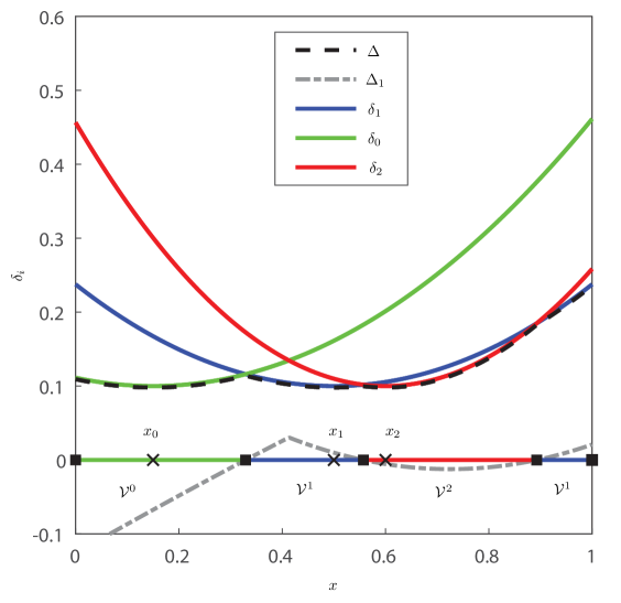
Figure 1: Illustration of the global lower envelope function $\Delta(x;X)$ for a network of three agents located in the interval $\mathcal{S}:=[0,1]$ together with the lower envelope function $\Delta_{1}(x;X)$ associated with agent $i=1$.

It is worth noting that for the computation of $\Delta_{i}(x;X)$, the $i$-th agent doesn’t need to know neither $x$ nor the set $X$ but instead the relative position $x-x_{i}$ and the positions of the other agents relative to itself (no global reference frame is required).

Proposition 7

Let $i\in[0,n]_{\bm{\mathbb{Z}}}$. There exists a function $\phi_{i}:\mathcal{S}\ominus\{x_{i}\}\rightarrow\mathbb{R}$ such that

$$\Delta_{i}(x;X)=\phi_{i}(x-x_{i};X\ominus\{x_{i}\}),~{}~{}\forall x\in\mathcal{S}.$$ (28)

Proof:

Indeed, for any $\ell\in[0,n]_{\bm{\mathbb{Z}}}\backslash\{i\}$, we have that

$$\delta_{\ell}(x;x_{\ell}) =(x-x_{\ell})^{\mbox{\scriptsize T}}\mathbf{P}_{\ell}(x-x_{\ell})+\mu_{\ell}$$

$$=(x-x_{i}+x_{i}-x_{\ell})^{\mbox{\scriptsize T}}\mathbf{P}_{\ell}(x-x_{i}+x_{i}-x_{\ell})+\mu_{\ell}$$

$$=(x-x_{i})^{\mbox{\scriptsize T}}\mathbf{P}_{\ell}(x-x_{i})+(x_{i}-x_{\ell})^{\mbox{\scriptsize T}}\mathbf{P}_{\ell}(x_{i}-x_{\ell})$$

$$~{}~{}~{}+2(x-x_{i})^{\mbox{\scriptsize T}}\mathbf{P}_{\ell}(x_{i}-x_{\ell})+\mu_{\ell}.$$

Therefore,

$$\Delta_{i}(x;X) =\min_{\ell\neq i}\big{(}(x-x_{i})^{\mbox{\scriptsize T}}\mathbf{P}_{\ell}(x-x_{i})$$

$$~{}~{}~{}\qquad~{}~{}+(x_{\ell}-x_{i})^{\mbox{\scriptsize T}}\mathbf{P}_{\ell}(x_{\ell}-x_{i})$$

$$~{}~{}~{}\qquad~{}~{}-2(x-x_{i})^{\mbox{\scriptsize T}}\mathbf{P}_{\ell}(x_{\ell}-x_{i})+\mu_{\ell}$$

$$~{}~{}~{}\qquad~{}~{}-(x-x_{i})^{\mbox{\scriptsize T}}\mathbf{P}_{i}(x-x_{i})-\mu_{i}\big{)}$$

$$=\min_{\ell\neq i}\big{(}(x-x_{i})^{\mbox{\scriptsize T}}(\mathbf{P}_{\ell}-\mathbf{P}_{i})(x-x_{i})$$

$$~{}~{}~{}\qquad~{}~{}+(x_{\ell}-x_{i})^{\mbox{\scriptsize T}}\mathbf{P}_{\ell}(x_{\ell}-x_{i})$$

$$~{}~{}~{}\qquad~{}~{}-2(x-x_{i})^{\mbox{\scriptsize T}}\mathbf{P}_{\ell}(x_{\ell}-x_{i})+\mu_{\ell}-\mu_{i}\big{)}.$$

Therefore, $\Delta_{i}(x;X)$ depends on the relative positions $x-x_{i}$ and $x_{i}-x_{\ell}$, for $\ell\neq i$. The result follows readily. ∎

• In light of Proposition 7, the computation of the $i$-th lower envelope $\Delta_{i}$ does not require a global reference frame but it does require, in principle, that all the agents communicate with each other in order to compute the quantity $\min_{\ell\neq i}\delta_{\ell}(x;x_{\ell})$ in a centralized way (all-to-all communication). Later on, however, we will see that the $i$-th agent can characterize $\Delta_{i}$ by communicating with only a subset of its teammates (the $i$-th agent will find the latter agents by discovering the network topology induced by the HQVP; the latter problem is addressed in Section V), and thus, the computation of $\Delta_{i}$ can take place in a distributed way.

III-C Parametrization of $\mathcal{V}^{i}$ and $\mathrm{bd}(\mathcal{V}^{i})$

Next, we will show that the cell $\mathcal{V}^{i}\in\mathcal{V}(X;\mathcal{S})$ and its boundary $\mathrm{bd}(\mathcal{V}^{i})$, for $i\in[1,n]_{\bm{\mathbb{Z}}}$, admit convenient parametrizations. These parametrizations will allow us to propose a systematic way to compute proxies of $\mathcal{V}^{i}$ and $\mathrm{bd}(\mathcal{V}^{i})$ in a finite number of steps. Before we proceed any further, we introduce some useful notation. In particular, for a given $i\in[1,n]_{\mathbb{Z}}$ and $\theta\in[0,2\pi[$, we will denote by $\Gamma_{\theta}$ the ray that starts from $x_{i}$ and is parallel to the unit vector $e_{\theta}=[\cos\theta,~{}\sin\theta]^{\mbox{\scriptsize T}}$, that is, $\Gamma_{\theta}:=\{x\in\mathbb{R}^{2}:~{}x=x_{i}+\rho e_{\theta},~{}\rho\geq 0\}$. In addition, we denote as $\overline{x}_{\theta}$ the point of intersection of $\Gamma_{\theta}$ with $\mathrm{bd}(E_{i}\cap\mathcal{S})$ where $E_{i}:=\mathcal{E}_{\ell_{i,0}}(\mathbf{P}_{i,0}^{-1}\chi_{i,0};\mathbf{P}_{i,0}^{-1})$.

In view of Proposition 6, to characterize $\mathrm{bd}(\mathcal{V}^{i})$ one has to find the roots of $\Delta_{i}=0$ in $E_{i}\cap\mathcal{S}$ and also check if $\mathrm{bd}(\mathcal{V}^{i})$ contains boundary points of $\mathcal{S}$. What we propose to do is to find the roots of $\Delta_{i}=0$ incrementally by searching along the ray $\Gamma_{\theta}$, or more precisely, the line segment $\Gamma_{\theta}\cap(E_{i}\cap\mathcal{S})=[x_{i},~{}\overline{x}_{\theta}]$, for a different $\theta\in[0,2\pi]$ at each time. For a given $\theta\in[0,2\pi]$, we will denote as $P_{\theta}^{i}$ the point-set comprised of the roots of the equation $\Delta_{i}=0$ in $[x_{i},~{}\overline{x}_{\theta}[$, that is,

$$P_{\theta}^{i}:=\{x\in[x_{i},~{}\overline{x}_{\theta}[:~{}\Delta_{i}(x;X)=0\}.$$ (29)

If $P_{\theta}^{i}\neq\varnothing$, then let $M:=\mathrm{card}(P_{\theta}^{i})$ and let us consider the ordered point-set

$$\mathfrak{P}_{\theta}^{i}=\{\mathfrak{p}_{m}\in[x_{i},~{}\overline{x}_{\theta}]:~{}m\in[0,M+1]_{\bm{\mathbb{Z}}}\},$$

which is comprised of the same points as the set $P_{\theta}^{i}\cup\{x_{i},\overline{x}_{\theta}\}$ with the latter points be arranged as follows:

$$\mathfrak{p}_{0}:=x_{i},~{}|x_{i}-\mathfrak{p}_{1}|<\dots<|x_{i}-\mathfrak{p}_{M}|,~{}\mathfrak{p}_{M+1}:=\overline{x}_{\theta}.$$ (30)

The points of $\mathfrak{P}_{\theta}^{i}$ determine a partition $\{I^{m}:m\in[1,M+1]_{\bm{\mathbb{Z}}}\}$, where $I^{m}:=[\mathfrak{p}_{m-1},~{}\mathfrak{p}_{m}]$, of the line segment $[x_{i},\overline{x}_{\theta}]$. Next, we provide one of the main results of this section regarding the characterization of the intersection of the cell $\mathcal{V}^{i}$ and its boundary $\mathrm{bd}(\mathcal{V}^{i})$ with the ray $\Gamma_{\theta}$.

Proposition 8

Let $i\in[1,n]_{\mathbb{Z}}$ and $\theta\in[0,2\pi]$. Let also $\{I^{m}:=[\mathfrak{p}_{m-1},~{}\mathfrak{p}_{m}]:m\in[1,M+1]_{\bm{\mathbb{Z}}}\}$ be the partition of $[x_{i},~{}\overline{x}_{\theta}]$ that is induced by the ordered point-set $\mathfrak{P}_{\theta}^{i}$ whose points are arranged according to (30). In addition, let $\hat{\mathfrak{p}}_{m}$ denote the midpoint of the line segment $I^{m}$ and let $\hat{\Delta}^{m}_{i}:=\Delta_{i}(\hat{\mathfrak{p}}_{m};X)$. Further, let us consider the index-sets

$$\mathcal{M}^{+} :=\{m\in[1,M+1]_{\bm{\mathbb{Z}}}:\hat{\Delta}^{m}_{i}>0\}$$

$$\mathcal{M}^{-} :=\{m\in[1,M+1]_{\bm{\mathbb{Z}}}:\hat{\Delta}^{m}_{i}<0\}.$$

Then,

$$\mathcal{V}^{i}\cap\Gamma_{\theta}=\mathfrak{f}_{\theta}(x_{i}),~{}~{}~{}\mathrm{bd}(\mathcal{V}^{i})\cap\Gamma_{\theta}=\mathfrak{g}_{\theta}(x_{i}),$$ (31)

where the set-valued maps $\mathfrak{f}_{\theta}(\cdot):X\rightrightarrows\wp([x_{i},~{}\overline{x}_{\theta}])$ and $\mathfrak{g}_{\theta}(\cdot):X\rightrightarrows\wp([x_{i},~{}\overline{x}_{\theta}])$ are defined as follows:

$\mathrm{i})$ If $P_{\theta}^{i}=\varnothing$, then

$$\mathfrak{f}_{\theta}(x_{i}):=[x_{i},\overline{x}_{\theta}],~{}~{}~{}\mathfrak{g}_{\theta}(x_{i}):=\{\overline{x}_{\theta}\}.$$

$\mathrm{ii})$ If $P_{\theta}^{i}\neq\varnothing$, then

$$\mathfrak{f}_{\theta}(x_{i}):=\bigcup_{m\in\mathcal{M}_{\mathfrak{f}}}I^{m},~{}~{}~{}\mathfrak{g}_{\theta}(x_{i}):=\{\mathfrak{p}_{m}:m\in\mathcal{M}_{\mathfrak{g}}\},$$

where $\mathcal{M}_{\mathfrak{f}}=\mathcal{M}^{+}$ and $\mathcal{M}_{\mathfrak{g}}:=\mathcal{M}_{\mathfrak{g}}^{+}\cup\mathcal{M}_{\mathfrak{g}}^{-}$. In particular, the index-set $\mathcal{M}_{\mathfrak{g}}^{+}$ is comprised of all $m\in\mathcal{M}^{+}\cap[1,M]_{\bm{\mathbb{Z}}}$ such that $m+1\in\mathcal{M}^{-}$ plus the index $M+1$ if $M+1\in\mathcal{M}^{+}$. Finally, the index-set $\mathcal{M}_{\mathfrak{g}}^{-}$ is comprised of all $m\in\mathcal{M}^{-}\cap[1,M]_{\bm{\mathbb{Z}}}$ such that $m+1\in\mathcal{M}^{+}$.

Proof:

First, we consider the case when $P_{\theta}^{i}=\varnothing$, that is, $\Delta_{i}$ has no roots in $[x_{i},\overline{x}_{\theta}[$. In view of Assumption 1, we have

$$\Delta_{i}(x_{i};X)=\min_{\ell\neq i}\delta_{\ell}(x_{i};x_{\ell})-\mu_{i}>0.$$

By continuity, we conclude that in this case $\Delta_{i}(x;X)>0$, for all $x\in[x_{i},\overline{x}_{\theta}[$, which implies that $\mathfrak{f}_{\theta}(x_{i})=\mathcal{V}^{i}\cap\Gamma_{\theta}=[x_{i},\overline{x}_{\theta}]$ and $\mathfrak{g}_{\theta}(x_{i})=\mathrm{bd}(\mathcal{V}^{i})\cap\Gamma_{\theta}=\{\overline{x}_{\theta}\}$.

Next, we consider the case when $P_{\theta}^{i}\neq\varnothing$. By definition, $\hat{\Delta}^{m}_{i}>0$ for all $m\in\mathcal{M}^{+}$. By continuity of $\Delta_{i}$, we have that $\Delta_{i}(x;X)\geq 0$ for all $x\in I_{m}=[\mathfrak{p}_{m-1},~{}\mathfrak{p}_{m}]$ and for all $m\in\mathcal{M}^{+}$. Therefore, in view of equation (26a), we have $\bigcup_{m\in\mathcal{M}_{\mathfrak{f}}}I_{m}=\mathcal{V}^{i}\cap\Gamma_{\theta}=\mathfrak{f}_{\theta}(x_{i})$ with $\mathcal{M}_{\mathfrak{f}}=\mathcal{M}^{+}$. Now, a point $\mathfrak{p}_{m}$ with $m\in[1,M]_{\bm{\mathbb{Z}}}$ belongs to $\mathrm{bd}(\mathcal{V}^{i})\cap\Gamma_{\theta}=\mathfrak{g}_{\theta}(x_{i})$ if and only if as one transverses $\Gamma_{\theta}$ (with direction from $x_{i}$ towards $\overline{x}_{\theta}$), one of the following two events takes place: 1) $\Delta_{i}$, which is negative “before” $\mathfrak{p}_{m}$, becomes positive “after” $\mathfrak{p}_{m}$ (in which case $m\in\mathcal{M}_{\mathfrak{g}}^{+}$) or 2) $\Delta_{i}$, which is positive “before” $\mathfrak{p}_{m}$, becomes negative “after” $\mathfrak{p}_{m}$ (in which case $m\in\mathcal{M}_{\mathfrak{g}}^{-}$). Finally, if $\Delta_{i}(\hat{\mathfrak{p}}_{M+1};X)>0$, then $\mathfrak{p}_{M+1}\in\mathfrak{g}_{\theta}(x_{i})$ and $M+1\in\mathcal{M}_{\mathfrak{g}}^{+}$. This completes the proof. ∎

Example: To better understand the implications of Proposition 8 as well as the meaning of each index-set introduced therein, let us consider the example illustrated in Figure 2. We have that $\mathfrak{P}_{\theta}^{i}=\{\mathfrak{p}_{m}:~{}m\in[0,5]_{\bm{\mathbb{Z}}}\}$ where $\mathfrak{p}_{0}\equiv x_{i}$ and $\mathfrak{p}_{5}\equiv\overline{x}_{\theta}$ and its induced partition is $\{I_{m}=[\mathfrak{p}_{m-1},\mathfrak{p}_{m}]:~{}m\in[1,5]_{\bm{\mathbb{Z}}}\}$. The sign of $\Delta_{i}$ at the mid-points of the segments $I_{1},I_{2},I_{4},I_{5}$, which are enclosed by dashed blue ellipses in the figure, is positive and thus $\mathcal{M}^{+}=\mathcal{M}_{\mathfrak{f}}=\{1,2,4,5\}$ whereas $\mathcal{M}^{-}=\{3\}$. We conclude that $\mathfrak{f}_{\theta}(x_{i})=[x_{i},\mathfrak{p}_{2}]\cup[\mathfrak{p}_{3},\overline{x}_{\theta}]$. Furthermore, as one transverses $\Gamma_{\theta}$ (from $x_{i}$ towards $\overline{x}_{\theta}$) $\Delta_{i}$ changes sign from positive to negative at $\mathfrak{p}_{2}$ and in addition, $\Delta_{i}>0$ at the mid-point of $I_{5}$; thus, $\mathcal{M}^{+}_{\mathfrak{g}}=\{2,5\}$. Also, $\Delta_{i}$ changes sign from negative to positive at $\mathfrak{p}_{3}$, and thus $\mathcal{M}^{-}_{\mathfrak{g}}=\{3\}$. Hence, $\mathcal{M}_{\mathfrak{g}}=\mathcal{M}_{\mathfrak{g}}^{+}\cup\mathcal{M}_{\mathfrak{g}}^{-}=\{2,3,5\}$. We conclude that $\mathfrak{g}_{\theta}(x_{i})=\{\mathfrak{p}_{2},\mathfrak{p}_{3},\mathfrak{p}_{5}\}$. The points from $\mathfrak{P}^{i}_{\theta}$ that form $\mathfrak{g}_{\theta}(x_{i})$ are encircled by blue circles in Figure 2.

• A careful interpretation of the results presented in Proposition 8 reveals that under some mild and intuitive modifications, one can characterize the cell $\mathcal{V}^{i}$ and its boundary $\mathrm{bd}(\mathcal{V}^{i})$ even for the more general case when Assumption 1 may not hold true. For instance, in the previous example, the sign of $\Delta_{i}$ in the segment $]x_{i},\mathfrak{p}_{1}[$ will not necessarily be positive (it is always positive if Assumption 1 holds true) and, instead, it will be equal to the sign of $\Delta_{i}$ at any interior point in that segment. For the sake of the argument, let us take the latter sign to be negative. Then, assuming that the signs of $\Delta_{i}$ in all the other segments remain the same as in Fig. 2, it follows that $\mathfrak{g}_{\theta}(x_{i})=\{\mathfrak{p}_{1},\mathfrak{p}_{2},\mathfrak{p}_{3},\mathfrak{p}_{5}\}$ and $\mathcal{M}^{+}=\mathcal{M}_{\mathfrak{f}}=\{2,4,5\}$.

Proposition 9

Let us consider a family of rays $\{\Gamma_{\theta}:~{}\theta\in[0,2\pi]\}$, where the ray $\Gamma_{\theta}$ emanates from $x_{i}$ and is parallel to the unit vector $e_{\theta}:=[\cos\theta,~{}\sin\theta]^{\mbox{\scriptsize T}}$. Then,

$$\mathcal{V}^{i} =\bigcup_{\theta\in[0,2\pi]}\mathfrak{f}_{\theta}(x_{i}),\qquad\mathrm{bd}(\mathcal{V}^{i})=\bigcup_{\theta\in[0,2\pi]}\mathfrak{g}_{\theta}(x_{i}),$$ (32)

where the set-valued maps $\mathfrak{f}_{\theta}(\cdot)$ and $\mathfrak{g}_{\theta}(\cdot)$ are defined as in Proposition 8 for each $\theta\in[0,2\pi]$.

Proof:

We have that

$$\bigcup_{\theta\in[0,2\pi]}\mathfrak{f}_{\theta}(x_{i})=\bigcup_{\theta\in[0,2\pi]}(\mathcal{V}^{i}\bigcap\Gamma_{\theta})=\mathcal{V}^{i}\bigcap(\bigcup_{\theta\in[0,2\pi]}\Gamma_{\theta})=\mathcal{V}^{i},$$

where in the first equality, we used (31) and in the last one, we used that $\bigcup_{\theta\in[0,2\pi]}\Gamma_{\theta}=\mathbb{R}^{2}$. Thus, we have proved that the first equation in (32) holds true. The proof for the second one follows similarly. ∎

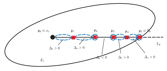
Figure 2: Illustrative example on the characterization of $\mathcal{V}^{i}\cap\Gamma_{\theta}$ and $\mathrm{bd}(\mathcal{V}^{i})\cap\Gamma_{\theta}$ based on Proposition 8.

IV A systematic approach for the computation of a finite approximation of $\mathrm{bd}(\mathcal{V}^{i})$ and $\mathcal{V}^{i}$

IV-A Efficient computation of the roots of the equation $\Delta_{i}=0$

In this section, we will leverage Propositions 8 and 9 to develop a systematic procedure to characterize the boundary points of $\mathcal{V}^{i}$ that lie on a given ray $\Gamma_{\theta}$ after a finite number of steps. To this aim, let $\overline{\rho}_{\theta}>0$ denote the length of $[x_{i},~{}\overline{x}_{\theta}]$, that is, $\overline{\rho}_{\theta}:=|\overline{x}_{\theta}-x_{i}|$. Recall that $\overline{x}_{\theta}$ corresponds to the intersection of $\Gamma_{\theta}$ with $\mathrm{bd}(E_{i}\cap\mathcal{S})$. In addition, let

$$\mathcal{R}^{i,j}_{\theta} :=\{\rho\in[0,~{}\overline{\rho}_{\theta}[:~{}\delta_{i}(x_{i}+\rho e_{\theta};x_{i})=$$

$$~{}~{}~{}~{}\qquad~{}~{}~{}~{}~{}~{}~{}~{}~{}~{}~{}~{}~{}~{}~{}~{}\delta_{j}(x_{i}+\rho e_{\theta};x_{j})\},$$ (33)

for $j\in[0,n]_{\mathbb{Z}}\backslash\{i\}$. Equivalently, $\mathcal{R}^{i,j}_{\theta}$ consists of all $\rho\in[0,~{}\overline{\rho}_{\theta}]$ that satisfy the following equation:

$$\alpha\rho^{2}+\beta\rho+\gamma=0,$$ (34)

where

$$\alpha :=|\bm{\Pi}_{i}^{1/2}e_{\theta}|^{2}-|\bm{\Pi}_{j}^{1/2}e_{\theta}|^{2},$$ (35a)

$$\beta :=2(x_{j}-x_{i})^{\mbox{\scriptsize T}}\bm{\Pi}_{j}e_{\theta},$$ (35b)

$$\gamma :=|\bm{\Pi}_{j}^{1/2}(x_{i}-x_{j})|^{2}+\mu_{i}-\mu_{j}.$$ (35c)

Note that if $\rho\in\mathcal{R}^{i,j}_{\theta}$, then the point $p:=x_{i}+\rho e_{\theta}$ will belong to $\Gamma_{\theta}\cap\mathcal{B}_{i,j}$. Let $\mathcal{P}^{i,j}_{\theta}:=\{p\in[x_{i},\overline{x}_{\theta}[:~{}p=x_{i}+\rho e_{\theta},~{}\rho\in\mathcal{R}^{i,j}_{\theta}\}$. Note that there is an (obvious) one-to-one correspondence between the point-sets $\mathcal{P}^{i,j}_{\theta}$ and $\mathcal{R}^{i,j}_{\theta}$, which may both be empty for some $j\neq i$. Now, let

$$\mathcal{R}^{i}_{\theta}:=\cup_{j\neq i}\mathcal{R}^{i,j}_{\theta},~{}~{}~{}~{}\mathcal{P}^{i}_{\theta}:=\cup_{j\neq i}\mathcal{P}^{i,j}_{\theta}.$$ (36)

Note that a point $p\in\mathcal{P}^{i}_{\theta}\backslash\{x_{i},\overline{x}_{\theta}\}$ is necessarily equidistant from the $i$-th agent and at least a different agent from the same extended network. This naturally leads us to the following proposition.

Proposition 10

Let $P^{i}_{\theta}$ be the point-set which is defined as in (29). Then, $\mathcal{P}^{i}_{\theta}\supseteq P^{i}_{\theta}$ and thus,

$$P^{i}_{\theta} =\{x\in\mathcal{P}^{i}_{\theta}:\Delta_{i}(x;X)=0\}.$$ (37)

Proof:

The proof follows readily from the definitions of $\mathcal{P}^{i}_{\theta}$ and $P^{i}_{\theta}$. ∎

Proposition 10 implies that for the characterization of the set $P^{i}_{\theta}$ that consists of all the roots of $\Delta_{i}=0$ in $[x_{i},\overline{x}_{\theta}[$, one has to evaluate the function $\Delta_{i}$ at the points of the finite point-set $\mathcal{P}^{i}_{\theta}$, which is a superset of the unknown set $P^{i}_{\theta}$. In particular, $P^{i}_{\theta}$ is comprised of all those points of $\mathcal{P}^{i}_{\theta}$ at which $\Delta_{i}$ vanishes and only them.

IV-B Line search algorithm for the computation of $\mathfrak{f}_{\theta}(x_{i})$ and $\mathfrak{g}_{\theta}(x_{i})$

Next, we present an algorithm that computes $\mathfrak{f}_{\theta}(x_{i})$ and $\mathfrak{g}_{\theta}(x_{i})$ for a given $\theta\in[0,2\pi[$ based on the previous discussion and analysis. The main steps of the proposed algorithmic process can be found in Algorithm 1. In particular, the first step is to compute the point-set $\mathcal{P}_{\theta}^{i}$ (line 5). If $\mathcal{P}^{i}_{\theta}=\varnothing$, then we set $\mathfrak{f}_{\theta}(x_{i})$ and $\mathfrak{g}_{\theta}(x_{i})$ to be equal to, respectively, $[x_{i},\overline{x}_{\theta}]$ and $\{\overline{x}_{\theta}\}$ and the process is complete (lines 6-7). If $\mathcal{P}^{i}_{\theta}\neq\varnothing$, we characterize all of the points in $\mathcal{P}^{i}_{\theta}$ that correspond to the roots of the equation $\Delta_{i}=0$ in $[x_{i},\overline{x}_{\theta}[$ to form the point-set $P_{\theta}^{i}$ in accordance with Proposition 10 (line 8). Next, we apply a permutation to the point-set $P_{\theta}^{i}\cup\{x_{i},\overline{x}_{\theta}\}$ to obtain the point-set $\mathfrak{P}_{\theta}^{i}=\{\mathfrak{p}_{m}:~{}m\in[1,M+1]_{\bm{\mathbb{Z}}}\}$ whose points are ordered in increasing distance from $x_{i}$ as in (30) (lines 9-10). Next, we start an iterative process for the characterization of the index sets $\mathcal{M}_{\mathfrak{f}}$ and $\mathcal{M}_{\mathfrak{g}}$, with $\mathcal{M}_{\mathfrak{f}}=\mathcal{M}^{+}$ and $\mathcal{M}_{\mathfrak{g}}=\mathcal{M}^{+}_{\mathfrak{g}}\cup\mathcal{M}^{-}_{\mathfrak{g}}$ (lines 11-25), where the index sets $\mathcal{M}^{+}$, $\mathcal{M}^{+}_{\mathfrak{g}}$ and $\mathcal{M}^{-}_{\mathfrak{g}}$ are defined as in Proposition 8. Finally, we set $\mathfrak{f}_{\theta}(x_{i}):=\cup_{m\in\mathcal{M}_{\mathfrak{f}}}[\mathfrak{p}_{m-1},\mathfrak{p}_{m}]$ and $\mathfrak{g}_{\theta}(x_{i}):=\{\mathfrak{p}_{m}\in\mathfrak{P}_{\theta}^{i}:~{}m\in\mathcal{M}_{\mathfrak{g}}\}$ (lines 26-27).

Note that after the computation of $\mathfrak{g}_{\theta}(x_{i})$, then, in view of Proposition 8, one can compute an approximation of $\mathrm{bd}(\mathcal{V}^{i})$ by computing $\mathfrak{g}_{\theta}(x_{i})$ for all $\theta\in\Theta$, where $\Theta$ is a finite point-set whose points define a partition of $[0,2\pi]$.

Algorithm 1 Computation of point-sets $\mathfrak{f}_{\theta}(x_{i})=\mathcal{V}^{i}\cap\Gamma_{\theta}$ and $\mathfrak{g}_{\theta}(x_{i})=\mathrm{bd}(\mathcal{V}^{i})\cap\Gamma_{\theta}$

1:procedure Cell computation

2:     Input data: $X$, $\{(\mathbf{P}_{\ell},\mu_{\ell}):~{}\ell\in[0,n]_{\bm{\mathbb{Z}}}\}$

3:     Input variables: $i$, $\theta$

4:     Output variables: $\mathfrak{f}_{\theta}(x_{i}),\mathfrak{g}_{\theta}(x_{i})$

5:     Find $\mathcal{P}^{i}_{\theta}$

6:     if $\mathcal{P}^{i}_{\theta}=\varnothing$ then

7:         $\mathfrak{f}_{\theta}(x_{i})\leftarrow[x_{i},\overline{x}_{\theta}]$, $\mathfrak{g}_{\theta}(x_{i})\leftarrow\{\overline{x}_{\theta}\}$ return      

8:     Extract point-set $P^{i}_{\theta}$ from $\mathcal{P}^{i}_{\theta}$ based on Proposition 10

9:     $\mathfrak{P}_{\theta}^{i}\leftarrow P^{i}_{\theta}\cup\{x_{i},\overline{x}_{\theta}\}$.

10:     Re-arrange points in $\mathfrak{P}_{\theta}^{i}=\{\mathfrak{p}_{m}:~{}m\in[0,M+1]_{\bm{\mathbb{Z}}}\}$ based on increasing distance from $x_{i}$ according to (30)

11:     $\mathcal{M}_{\mathfrak{f}}\leftarrow\varnothing,~{}\mathcal{M}_{\mathfrak{g}}^{+}\leftarrow\varnothing,~{}\mathcal{M}_{\mathfrak{g}}^{-}\leftarrow\varnothing$

12:     for  $m=1:M+1$ do

13:         $\hat{x}\leftarrow\tfrac{1}{2}(\mathfrak{p}_{m-1}+\mathfrak{p}_{m})$ $\triangleright$ $\hat{x}$: midpoint of $I^{m}$

14:         $\hat{\Delta}\leftarrow\Delta_{i}(\hat{x};X)$

15:         if $\hat{\Delta}>0$ then $\mathcal{M}_{\mathfrak{f}}\leftarrow\mathcal{M}_{\mathfrak{f}}\cup\{m\}$          

16:         if  $m<M+1$ then

17:              $\hat{x}^{\prime}\leftarrow\tfrac{1}{2}(\mathfrak{p}_{m}+\mathfrak{p}_{m+1})$ $\triangleright$ $\hat{x}^{\prime}$: midpoint of $I^{m+1}$

18:              $\hat{\Delta}^{\prime}\leftarrow\Delta_{i}(\hat{x}^{\prime};X)$

19:              if  $\hat{\Delta}>0$ and $\hat{\Delta}^{\prime}<0$  then

20:                  $\mathcal{M}_{\mathfrak{g}}^{+}\leftarrow\mathcal{M}_{\mathfrak{g}}^{+}\cup\{m\}$               

21:              if  $\hat{\Delta}<0$ and $\hat{\Delta}^{\prime}>0$  then

22:                  $\mathcal{M}_{\mathfrak{g}}^{-}\leftarrow\mathcal{M}_{\mathfrak{g}}^{-}\cup\{m\}$                        

23:         if  $\hat{\Delta}>0$ and $m=M+1$ then

24:              $\mathcal{M}^{+}_{\mathfrak{g}}\leftarrow\mathcal{M}^{+}_{\mathfrak{g}}\cup\{m\}$               

25:     $\mathcal{M}_{\mathfrak{g}}\leftarrow\mathcal{M}^{+}_{\mathfrak{g}}\cup\mathcal{M}^{-}_{\mathfrak{g}}$

26:     $\mathfrak{f}_{\theta}(x_{i})\leftarrow\{[\mathfrak{p}_{m-1},\mathfrak{p}_{m}]:~{}m\in\mathcal{M}_{\mathfrak{f}}\}$

27:     $\mathfrak{g}_{\theta}(x_{i})\leftarrow\{\mathfrak{p}_{m}:~{}m\in\mathcal{M}_{\mathfrak{g}}\}$

V Discovery of Network Topology Induced by HQVP

In order to solve Problem 1 in a distributed way, it is necessary that the $i$-th agent can discover a superset of its neighbors in the topology of HQVP before even computing its own cell. Next, we characterize an upper bound on the distance of the $i$-th agent, measured in terms of $\delta_{i}$, from the points in its own cell.

Proposition 11

Let $E_{i}:=\mathcal{E}_{\ell_{i,0}}(\mathbf{P}_{i,0}^{-1}\chi_{i,0};\mathbf{P}_{i,0}^{-1})$. Then,

$$\delta_{i}(x;x_{i})\leq\overline{\delta}_{i},~{}~{}~{}\forall~{}x\in\mathcal{V}^{i},$$ (38)

where $\overline{\delta}_{i}:=\max\{\delta_{i}(x;x_{i}):~{}x\in\mathrm{bd}(E_{i}\cap\mathcal{S})\}$.

Proof:

Because $\delta_{i}(x;x_{i})$ is a convex quadratic function, we conclude that its restriction over the convex and compact set $E_{i}\cap\mathcal{S}$ attains its maximum value in the latter set and in addition, at least one of its maximizers belongs to the boundary $\mathrm{bd}(E_{i}\cap\mathcal{S})$ of the same set. Consequently,

$$\overline{\delta}_{i} =\max\{\delta_{i}(x;x_{i}):~{}x\in E_{i}\cap\mathcal{S}\}$$

$$=\max\{\delta_{i}(x;x_{i}):~{}x\in\mathrm{bd}(E_{i}\cap\mathcal{S})\}.$$

Inequality (38) follows from the set inclusion (21). ∎

Proposition 12

Let us consider the index-set $\widetilde{\mathcal{N}}_{i}$ which is defined as follows:

$$\widetilde{\mathcal{N}}_{i}:=\{\ell\in[0,n]_{\bm{\mathbb{Z}}}\backslash\{i\}:\delta_{\ell}(x;x_{\ell})\leq\overline{\delta}_{i},~{}\forall x\in\mathrm{bd}(E_{i}\cap\mathcal{S})\},$$

where $\overline{\delta}_{i}:=\max\{\delta_{i}(x;x_{i}):~{}x\in\mathrm{bd}(E_{i}\cap\mathcal{S})\}$. Then, the set inclusion $\widetilde{\mathcal{N}}_{i}\supseteq\mathcal{N}_{i}$ holds true.

Proof:

In view of Proposition 2, all points in $\mathrm{bd}(\mathcal{V}^{i})\backslash\mathrm{bd}(\mathcal{S})$ are equidistant from at least one different agent from the same network, that is, for any point $x\in\mathrm{bd}(\mathcal{V}^{i})\backslash\mathrm{bd}(\mathcal{S})$, there exists $j_{x}\in[0,n]_{\bm{\mathbb{Z}}}\backslash\{i\}$ (the index $j_{x}$ depends on $x$) such that $\delta_{i}(x;x_{i})=\delta_{j_{x}}(x;x_{j_{x}})$. Thus, in view of Definition 2, $j_{x}\in\mathcal{N}_{i}$. Now let $\ell\neq i$ and let us assume that $\ell\in\widetilde{\mathcal{N}}_{i}^{c}$, where $\widetilde{\mathcal{N}}_{i}^{c}:=\{\ell\in[0,n]_{\bm{\mathbb{Z}}}\backslash\{i\}:\ell\notin\widetilde{\mathcal{N}}_{i}\}$. Then, $\delta_{\ell}(x;x_{\ell})>\overline{\delta}_{i}$, $\forall x\in\mathrm{bd}(E_{i}\cap\mathcal{S})$. But, in view of Proposition 11, $\delta_{i}(x;x_{i})\leq\overline{\delta}_{i},~{}~{}\forall x\in\mathcal{V}^{i}\supsetneq\mathrm{bd}(\mathcal{V}^{i})$; consequently, there is no point $x\in\mathrm{bd}(\mathcal{V}^{i})$ such that $\delta_{i}(x;x_{i})=\delta_{\ell}(x;x_{\ell})$. Thus, $\ell\in\mathcal{N}_{i}^{c}$ where $\mathcal{N}_{i}^{c}:=\{\ell\in[0,n]_{\bm{\mathbb{Z}}}\backslash\{i\}:\ell\notin\mathcal{N}_{i}\}$, which implies that $\widetilde{\mathcal{N}}_{i}^{c}\subseteq\mathcal{N}_{i}^{c}$. We conclude that $\widetilde{\mathcal{N}}_{i}\supseteq\mathcal{N}_{i}$ and the proof is complete. ∎

Next, we will leverage Proposition 12 to show that the $i$-th agent can find a subset of the spatial domain $\mathcal{S}$ that will necessarily contain its neighbors without having computed $\mathcal{V}^{i}$.

Proposition 13

Let $i\in[1,n]_{\bm{\mathbb{Z}}}$ and let $\mathcal{A}_{i}$ denote the compact set enclosed by the closed curve $\mathcal{C}_{i}:[0,2\pi]\rightarrow\mathbb{R}^{2}$ with

$$\mathcal{C}_{i}(\phi) :=\mathbf{P}_{i,0}^{-1}\chi_{i,0}+\sqrt{\ell_{i,0}}\mathbf{P}_{i,0}^{-1/2}e_{\phi}$$

$$~{}~{}~{}~{}+(\sqrt{r}/\|\mathbf{P}_{0}^{-1/2}\mathbf{P}_{i,0}^{1/2}e_{\phi}\|)\mathbf{P}_{0}^{-1}\mathbf{P}_{i,0}^{1/2}e_{\phi},$$ (39)

where $e_{\phi}:=[\cos\phi,~{}\sin\phi]^{\mathrm{T}}$. Then, all the neighbors of the $i$-th agent lie necessarily in $\mathcal{A}_{i}$, that is,

$$x_{\ell}\in\mathcal{A}_{i}\cap X,~{}~{}~{}\forall~{}\ell\in\mathcal{N}_{i}.$$ (40)

Proof:

Let $\mathsf{w}\in\mathrm{bd}(E_{i})$, where $E_{i}:=\mathcal{E}_{\ell_{i,0}}(\mathbf{P}_{i,0}^{-1}\chi_{i,0};\mathbf{P}_{i,0}^{-1})$, and let us consider a point $\mathsf{z}$ such that the intersection of the ellipsoid $\mathcal{E}_{r_{i}}(\mathsf{z};\mathbf{P}_{0}^{-1})$, where $r_{i}:=\overline{\delta}_{i}-\mu_{0}$ (note that $r_{i}>0$ in view of Assumption 2), with $E_{i}$ corresponds to the singleton $\{\mathsf{w}\}$, that is,

$$\{\mathsf{w}\} =E_{i}\cap\mathcal{E}_{r_{i}}(\mathsf{z};\mathbf{P}_{0}^{-1})=\mathrm{bd}(E_{i})\cap\mathrm{bd}(\mathcal{E}_{r_{i}}(\mathsf{z};\mathbf{P}_{0}^{-1})).$$

Because $\mathsf{w}\in\mathrm{bd}(E_{i})\cap\mathrm{bd}(\mathcal{E}_{r_{i}}(\mathsf{z};\mathbf{P}_{0}^{-1}))$,

$$0 =\|\mathbf{P}_{i,0}^{1/2}(\mathsf{w}-\mathbf{P}_{i,0}^{-1}\chi_{i,0})\|-\sqrt{\ell_{i,0}}=\|\mathbf{P}_{0}^{1/2}(\mathsf{w}-\mathsf{z})\|-\sqrt{r_{i}},$$

which implies that there exist $\phi,\varphi\in[0,2\pi[$ such that

$$\mathsf{w}=\mathbf{P}_{i,0}^{-1}\chi_{i,0}+\sqrt{\ell_{i,0}}\mathbf{P}_{i,0}^{-1/2}e_{\phi}=\mathsf{z}+\sqrt{r_{i}}\mathbf{P}_{0}^{-1/2}e_{\varphi},$$

where $e_{\phi}:=[\cos\phi,~{}\sin\phi]^{\mathrm{T}}$ and $e_{\varphi}:=[\cos\varphi,~{}\sin\varphi]^{\mathrm{T}}$. Thus,

$$\mathsf{z}=\mathbf{P}_{i,0}^{-1}\chi_{i,0}+\sqrt{\ell_{i,0}}\mathbf{P}_{i,0}^{-1/2}e_{\phi}-\sqrt{r_{i}}\mathbf{P}_{0}^{-1/2}e_{\varphi}.$$

The normal vectors of the ellipsoids $E_{i}$ and $\mathcal{E}_{r_{i}}(\mathsf{z};\mathbf{P}_{0}^{-1})$ at point $\mathsf{w}$ (contact point) are anti-parallel, that is, there exists $\lambda>0$ such that

$$\tfrac{\partial}{\partial x}\big{(}(x-\mathbf{P}_{i,0}^{-1}\chi_{i,0})^{\mbox{\scriptsize T}}\mathbf{P}_{i,0}(x-\mathbf{P}_{i,0}^{-1}\chi_{i,0})-\ell_{i,0}\big{)}\big{|}_{x=\mathsf{w}}$$

$$~{}~{}\qquad~{}~{}~{}\qquad~{}~{}=-\lambda\tfrac{\partial}{\partial x}\big{(}(x-\mathsf{z})^{\mbox{\scriptsize T}}\mathbf{P}_{0}(x-\mathsf{z})-r_{i}\big{)}\big{|}_{x=\mathsf{w}},$$

from which it can be shown (see, for instance, Lemma 5 in [35]) that

$$e_{\varphi}=-(1/\|\mathbf{P}_{0}^{-1/2}\mathbf{P}_{i,0}^{1/2}e_{\phi}\|)\mathbf{P}_{0}^{-1/2}\mathbf{P}_{i,0}^{1/2}e_{\phi}$$

and thus, we conclude that $\mathsf{z}=\mathcal{C}_{i}(\phi)$ where $\mathcal{C}_{i}(\phi)$ is defined in (13).

Now, let $\mathcal{A}_{i}$ be the compact set enclosed by the closed curve $\mathcal{C}_{i}$. We will show that all the neighbors of the $i$-th agent are located in $\mathcal{A}_{i}$, that is, $\mathcal{A}_{i}\supsetneq\{x_{k}\in X:~{}k\in\mathcal{N}_{i}\}$. In view of Proposition 1, the set inclusion $\mathcal{E}_{r_{i}}(\mathsf{z};\mathbf{P}_{0}^{-1})\supsetneq\mathcal{E}_{r_{i}}(\mathsf{z};\mathbf{P}_{\ell}^{-1})$ holds true for all $\mathsf{z}\in\mathcal{C}_{i}$ and for all $\ell\neq i$. Now, for a given $\mathsf{z}\in\mathcal{C}_{i}$, we have that

$$\delta_{0}(x;\mathsf{z})=(x-\mathsf{z})^{\mbox{\scriptsize T}}\mathbf{P}_{0}(x-\mathsf{z})+\mu_{0}=\overline{\delta}_{i},$$

for all $x\in\mathrm{bd}(\mathcal{E}_{r_{i}}(\mathsf{z};\mathbf{P}_{0}^{-1}))$ whereas

$$\delta_{\ell}(y;\mathsf{z})=(y-\mathsf{z})^{\mbox{\scriptsize T}}\mathbf{P}_{\ell}(y-\mathsf{z})+\mu_{\ell}=\overline{\delta}_{i}+\mu_{\ell}-\mu_{0},$$

for all $y\in\mathrm{bd}(\mathcal{E}_{r_{i}}(\mathsf{z};\mathbf{P}_{\ell}^{-1}))$. Because, $\mu_{\ell}-\mu_{0}\geq 0$, we conclude that $\max\{\delta_{\ell}(y;\mathsf{z}):y\in\mathcal{E}_{r_{i}}(\mathsf{z};\mathbf{P}_{\ell}^{-1})\}\geq\max\{\delta_{0}(x;\mathsf{z}):x\in\mathcal{E}_{r_{i}}(\mathsf{z};\mathbf{P}_{0}^{-1})\}$ which together with the set inclusion $\mathcal{E}_{r_{i}}(\mathsf{z};\mathbf{P}_{0}^{-1})\supsetneq\mathcal{E}_{r_{i}}(\mathsf{z};\mathbf{P}_{\ell}^{-1})$ imply that $\delta_{\ell}(y;\mathsf{z})>\overline{\delta}_{i}$ for all $y\in E_{i}\supseteq E_{i}\cap\mathcal{S}\supseteq\mathcal{V}^{i}$ (the last set inclusion follows from Proposition 5). Therefore,

$$\delta_{\ell}(x;\mathsf{z})>\overline{\delta}_{i}\geq\max\{\delta_{\ell}(y;x_{i}):~{}y\in\mathcal{V}^{i}\},~{}~{}~{}\forall x\in\mathcal{V}^{i}.$$ (41)

Therefore, there is no point $x\in\mathrm{\mathrm{bd}}(\mathcal{V}^{i})$ such that $\delta_{\ell}(x;\mathsf{z})=\delta_{\ell}(x;x_{i})$ for any $\mathsf{z}\in\mathcal{C}_{i}$. Thus, in view of Proposition 2, it follows that $\ell\notin\mathcal{N}_{i}$ and the proof is complete. ∎

Proposition 13 implies that the neighbors of the $i$-th agent are necessarily confined in the subset $\mathcal{A}_{i}\subseteq\mathcal{S}$ which is known to this agent before computing its cell $\mathcal{V}^{i}$. In practice, the $i$-th agent can communicate and exchange information directly with its neighbors (e.g., by means of point-to-point communication) provided that its communication radius $\eta_{i}>0$ is sufficiently large such that its communication region $\mathcal{B}_{\eta_{i}}(x_{i})\supseteq\mathcal{A}_{i}$.

Proposition 14

The neighbors of the $i$-th agent are necessarily located in the communication region $\mathcal{B}_{\eta_{i}}(x_{i})$ of the $i$-th agent, that is,

$$\mathcal{B}_{\eta_{i}}(x_{i})\supseteq\{x_{k}\in X:~{}k\in\mathcal{N}_{i}\},~{}~{}~{}~{}\forall\eta_{i}\geq\underline{\eta_{i}}$$ (42)

where $\underline{\eta_{i}}:=\max_{\phi\in[0,2\pi]}\|\mathcal{C}_{i}(\phi)-x_{i}\|$, with $\mathcal{C}_{i}(\phi)$ defined as in (13).

Proof:

By the definition of $\underline{\eta_{i}}$, we have that

$$\mathcal{B}_{\eta_{i}}(x_{i})\supsetneq\{\mathcal{C}_{i}(\phi):~{}\phi\in[0,2\pi]\}=\mathrm{bd}(\mathcal{A}_{i}),$$

and thus $\mathcal{B}_{\eta_{i}}(x_{i})\supseteq\mathcal{A}_{i}$, for all $\eta_{i}\geq\underline{\eta_{i}}$. Because $\mathcal{A}_{i}$ contains all the neighbors of the $i$-th agent in view of Proposition 13, then so does the closed ball $\mathcal{B}_{\eta_{i}}(x_{i})$, for any $\eta_{i}\geq\underline{\eta_{i}}$. Thus, the set inclusion (42) holds true. ∎

Proposition 15

Let $\mathcal{I}\subseteq\mathcal{N}_{i}\subseteq\widetilde{\mathcal{N}}_{i}\subseteq[0,n]_{\mathbb{Z}}$, where the index sets $\mathcal{N}_{i}$ and $\widetilde{\mathcal{N}}_{i}$ are defined as in (6) and Proposition 12, respectively, and let $\Delta_{i}^{\mathcal{I}}(x):=\min_{\ell\in\mathcal{I}\backslash\{i\}}\delta_{\ell}(x;x_{\ell})-\delta_{i}(x;x_{i})$. Then

$$\Delta_{i}^{\mathcal{I}}(x;x_{i})=\Delta_{i}(x;x_{i})=0,~{}~{}~{}\forall x\in\mathrm{bd}(\mathcal{V}^{i})\backslash\mathrm{bd}(\mathcal{S}),$$ (43)

where $\Delta_{i}(x;x_{i})$ is defined as in (24).

Proof:

By definition, $\Delta_{i}^{\mathcal{I}}(x)\geq\Delta_{i}(x;X)$, for all $x\in\mathcal{S}$, given that the $\min$ operator in the definition of $\Delta_{i}^{\mathcal{I}}$ is applied over an index set which is a subset of the one that appears in the definition of $\Delta_{i}$ in (24). In addition, in view of Prop. 6, $\Delta_{i}(x;X)=0$ for all $\mathrm{bd}(\mathcal{V}^{i})\backslash\mathrm{bd}(\mathcal{S})$, which implies that $\Delta_{i}^{\mathcal{I}}(x)\geq 0$ for all $x\in\mathrm{bd}(\mathcal{V}^{i})\backslash\mathrm{bd}(\mathcal{S})$. Next, we show that the previous non-strict inequality can only hold as an equality. Let us assume that there exists $z\in\mathrm{bd}(\mathcal{V}^{i})\backslash\mathrm{bd}(\mathcal{S})$ such that $\Delta_{i}^{\mathcal{I}}(z)>0$. However, since $\Delta_{i}(z;X)=0$, there is $j_{z}\notin\mathcal{I}$ such that $\delta(z;x_{i})=\delta(z;x_{j_{z}})$, which implies that the agent $j_{z}$ is a neighbor of the $i$-th agent, or equivalently, $j_{z}\in\mathcal{N}_{i}$. However, $j_{z}\notin\mathcal{I}$ and we know that, by hypothesis, $\mathcal{I}\subseteq\mathcal{N}_{i}$; thus, we have reached a contradiction and the proof is complete. ∎

• Proposition 15 implies that the Voronoi cell $\mathcal{V}^{i}$ and its boundary $\mathrm{bd}(\mathcal{V}^{i})$, which are fully characterized in Proposition 8, can be computed in a distributed way that relies on the exchange of information of the $i$-th agent with only the set of agents whose index belongs to $\widetilde{\mathcal{N}}_{i}\supseteq\mathcal{N}_{i}$ (the latter set of agents contains necessarily the set of neighbors of the $i$-th agent in view of Proposition 12). In other words, the cell $\mathcal{V}^{i}$ and its boundary $\mathrm{bd}(\mathcal{V}^{i})$ can be computed in a distributed way, which is a key result of this work.

• Let us assume that the $i$-th agent can communicate with all of its teammates in order to compute the point-set $P_{\theta}^{i}$, which according to Proposition 8 plays a key role in the complete characterization of $\mathcal{V}^{i}$ and $\mathrm{bd}(\mathcal{V}^{i})$. For a given $\theta\in[0,2\pi[$, the point-set $P_{\theta}^{i}$ will consist of $M$ points, which means that the $i$-th agent will have to exchange at least $M$ messages with the other agents from the same network, under the assumption of an all-to-all type communication. To each pair $(i,j)$ corresponds at most two points in $P_{\theta}^{i}$ (note that the quadratic equation (34) has at most 2 solutions whose corresponding points $p=x_{i}+\rho e_{\theta}$ can lie in $\mathcal{S}$). Thus, in the worst case, $M=2n$ assuming the exchange of 2 messages for each un-ordered pair $(i,j)$. The most expensive part of the proposed partitioning algorithm is the ordering of the points in $P_{\theta}^{i}$ in accordance with (30) to construct the (ordered) point-set $\mathfrak{P}_{\theta}^{i}$. The process of ordering the point-set $P_{\theta}^{i}$ (equivalent to sorting a list) has worst-case time complexity in $\mathcal{O}(M\mathrm{ln}(M))$ or $\mathcal{O}(2n\mathrm{ln}(2n))$. Let $n_{i}$ denote the number of the agents which are located in the set $\mathcal{A}_{i}$, which according to Prop.  13 contains the locations of all the neighbors of the $i$-th agent. Now, let $\zeta_{i}=n_{i}/n$, then the number of messages that the $i$-th agent has to exchange is $\zeta_{i}M$ and the worst-time complexity for ordering the points of $P_{\theta}^{i}$ that lie in $\mathcal{A}_{i}$ in accordance with (30) is in $\mathcal{O}(2\zeta_{i}n\,\mathrm{ln}(2\zeta_{i}n))$.

VI Numerical Simulations

We consider a heterogeneous multi-agent network of $n=24$ agents (plus the $0$-th agent) with different distance operators. For our simulations, we consider the spatial domain $\mathcal{S}=[-4,4]\times[-4,4]$ and we take $\mathbf{P}_{i}=\mathbf{U}_{i}\mathbf{D}\mathbf{U}_{i}^{\mbox{\scriptsize T}}$, with $\mathbf{D}=\big{[}\begin{smallmatrix}8&0\\ 0&3\end{smallmatrix}\big{]}$ and $\mathbf{U}_{i}=\big{[}\begin{smallmatrix}\cos\phi_{i}&-\sin\phi_{i}\\ \sin\phi_{i}&\cos\phi_{i}\end{smallmatrix}\big{]}$, where $\phi_{i}=2\pi i/n$, for $i\in[1,n]_{\bm{\mathbb{Z}}}$, and $\mu_{i}=0$ for all $i\in[1,n]_{\bm{\mathbb{Z}}}$. Clearly, $\lambda_{\min}(\mathbf{P}_{i})=3$ and $\lambda_{\max}(\mathbf{P}_{i})=8$ for all $i\in[1,n]$ and thus, the ratio $\lambda_{\max}(\mathbf{P}_{i})/\lambda_{\min}(\mathbf{P}_{i})=8/3$, which indicates the presence of strong anisotropic features. Furthermore, we take $x_{0}=(1/n)x_{i}$ (average position of the agents of the actual network), $\mathbf{P}_{0}=\lambda_{0}\mathbf{I}$ with $\lambda_{0}\in\{1.7,2.9\}$ and $\mu_{0}=0$ (note that $0<\lambda_{0}<\lambda_{\min}(\mathbf{P}_{i})$ for all $i\in[1,n]_{\bm{\mathbb{Z}}}$). With this particular selection of parameters, both Assumptions 1 and 2 are clearly satisfied. The HQVPs generated by the positions of the extended network are illustrated in Fig. 3(a) for $\lambda_{0}=1.7$ and in Fig. 3(b) for $\lambda_{0}=2.9$. The partitions in Figure 3 have been computed by means of exhaustive numerical techniques and the obtained results are included here mainly for verification purposes. In the same figure, we have included contours (level sets) of the proximity metric of each agent restricted on their own cells to illustrate the anisotropic features in this partitioning problem. The cell $\mathcal{V}^{0}$ corresponds to the red cell which is placed near the center of the spatial domain $\mathcal{S}$. We observe that $\mathcal{V}^{0}$ is smaller when $\lambda_{0}=2.9$ than when $\lambda_{0}=1.7$. Note that by letting $\lambda_{0}$ get closer (from below) to $\lambda_{\min}(\mathbf{P}_{i})=3$, the matrix $\mathbf{P}_{0}$ gets “closer” to violating Assumption 2 whereas the coverage hole $\mathcal{V}^{0}$ becomes smaller. Thus, selection of $\lambda_{0}$ has to strike a balance between well-posedness of the proposed partitioning algorithm and smallness of the coverage hole $\mathcal{V}^{0}$. Another interesting observation is that the cell $\mathcal{V}^{15}$ in both partitions is comprised of two disconnected components (only one of them contains in its interior the corresponding generator $x_{15}$).

Figure 4 illustrates the cells $\mathcal{V}^{14}$ and $\mathcal{V}^{23}$ of the HQVP computed by means of the proposed distributed algorithm for $\lambda_{0}=1.7$ (Figs. 4(a)-4(b)) and $\lambda_{0}=2.9$ (Figs. 4(c)-4(d)). For these simulations, we have used a uniform grid of $[0,2\pi[$ comprised of 360 nodes for the parameter (angle) $\theta$. The cross markers denote the generators $x_{14}$ and $x_{23}$ whereas the small red circles and red disks correspond to the positions of the rest of the agents of the extended network. In particular, the red (filled) disks in Fig. 4 correspond to the neighbors of the $i$-th agent in the topology of the HQVP, for $i=14$ and $i=23$, respectively. The red dashed-dotted curves in the same figures indicate the boundaries of the ellipsoids $E_{14}$ and $E_{23}$ (recall that the latter ellipsoids contain the cells $\mathcal{V}^{14}$ and $\mathcal{V}^{23}$ in view of Proposition 4) whereas the blue dashed curves denote the boundaries of the sets $\mathcal{A}_{14}$ and $\mathcal{A}_{23}$ which contain the neighbors of the $i$-th agent for, respectively, $i=14$ and $i=23$ in view of Proposition 13. We observe that the cells $\mathcal{V}^{14}$ and $\mathcal{V}^{23}$ in Fig. 4 match with their corresponding cells in Fig. 3(a). In addition, the results illustrated in Fig. 4(a) –4(d) are in agreement with Propositions 5 and 13. In particular, the ellipsoids $E_{14}$ and $E_{23}$ contain, respectively, the cells $\mathcal{V}^{14}$ and $\mathcal{V}^{23}$. Furthermore, the sets $\mathcal{A}_{14}$ and $\mathcal{A}_{23}$ contain the neighbors of the $i$-th agent for, respectively, $i=14$ and $i=23$, which are denoted as filled red disks.

We observe that the sets $E_{14}$, $E_{23}$, $\mathcal{A}_{14}$ and $\mathcal{A}_{23}$ in Figs. 4(a)-4(b) (corresponding to $\lambda_{0}=1.7$) are significantly smaller than their counterparts in Figs. 4(c)-4(d) (corresponding to $\lambda_{0}=2.9$). We conclude that although the decrease of the value of the parameter $\lambda_{0}$ may increase the size of the coverage hole (cell $\mathcal{V}^{0}$), it may, on the other hand, render the problem of discovering the network topology induced by HQVP more meaningful in the sense that by solving the latter problem each agent will be able to identify a rather small subset of the spatial domain that necessarily contains its neighbors. In this way, each agent will be able to avoid communicating with non-neighboring agents which cannot contribute to the process of computing its own cells. In our simulations, we observe that while the cells $\mathcal{V}^{14}$ for $\lambda_{0}=1.7$ and $\lambda_{0}=2.9$ are identical and their agents have the exact same sets of neighbors in both cases, the agent $i=14$ has to communicate with more agents (the ones that lie within the set $\mathcal{A}_{14}$ in view of Prop. 13) and also search for the boundary points of its own cell over a larger set (in view of the Prop. 5, $\mathcal{V}^{14}$ is a subset of $E_{14}$) when $\lambda_{0}=2.9$ than when $\lambda_{0}=1.7$. The situation is similar for $\mathcal{V}^{23}$ although the changes on the sets $E_{23}$ and $\mathcal{A}_{23}$ have a less substantial effect mainly because the agent $i=23$ is isolated from the majority of its teammates and is located close to the boundary of the spatial domain $\mathcal{S}$.

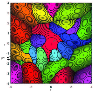
(a) $\mathbf{P}_{0}=1.7\mathbf{I}$

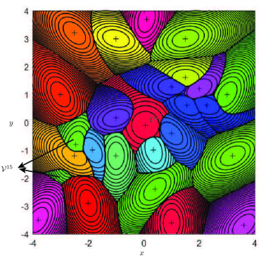
(b) $\mathbf{P}_{0}=2.9\mathbf{I}$

Figure 3: The HQVP generated by a heterogeneous network of $n=24$ agents (plus the $0$-th agent).

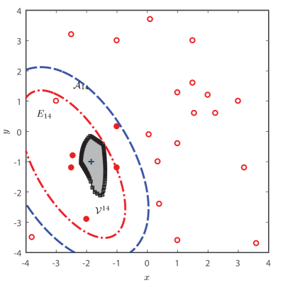
(a) $i=14$ ($\lambda_{0}=1.7$)

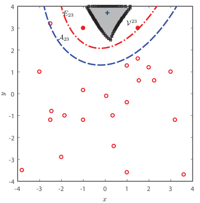
(b) $i=23$ ($\lambda_{0}=1.7$)

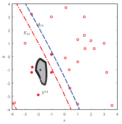
(c) $i=14$ ($\lambda_{0}=2.9$)

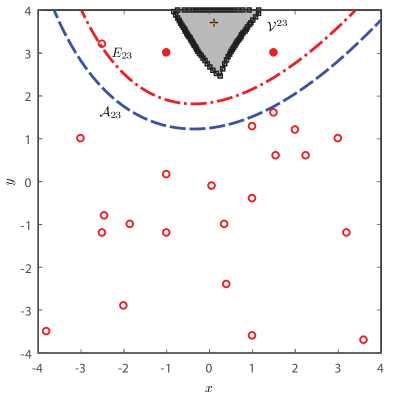
(d) $i=23$ ($\lambda_{0}=2.9$)

Figure 4: The cells $\mathcal{V}^{14}$ and $\mathcal{V}^{23}$ of the HQVP computed independently by means of the proposed partitioning algorithm together with their corresponding sets $E_{14}$, $\mathcal{A}_{14}$ and $E_{23}$, $\mathcal{A}_{23}$ for $\lambda_{0}=1.7$ (Figs. 4(a)-4(b)) and $\lambda_{0}=2.9$ (Figs. 4(c)-4(d)). The boundaries of the ellipsoidal sets $E_{14}$ and $E_{23}$ (these sets are a priori known bounds of $\mathcal{V}^{14}$ and $\mathcal{V}^{23}$, respectively) are denoted as red dash-dotted curves whereas the boundaries of the sets $\mathcal{A}_{14}$ and $\mathcal{A}_{23}$, which necessarily include the neighboring agents (red filled disks) of agents $i=14$ and $i=23$, are denoted as blue dashed curves.

VII Conclusion

In this work, we have presented distributed algorithms for workspace partitioning and network topology discovery problems for heterogeneous multi-agent networks whose agents employ different quadratic proximity metrics. The proposed algorithms leverage the underlying structure of the solutions to the problems considered. In our future work, we will explore how the proposed algorithms can be integrated in solution techniques for distributed optimization and estimation problems for heterogeneous networks operating in anisotropic environments.

References

- [1] F. Labelle and J. R. Shewchuk, “Anisotropic Voronoi diagrams and guaranteed quality anisotropic mesh generation,” in SCG’ 03, pp. 191–200, 2003.
- [2] S. P. Lloyd, “Least squares quantization in PCM,” IEEE Transactions on Information Theory, vol. 28, no. 2, pp. 129–137, 1982.
- [3] J. Cortes, S. Martinez, T. Karatas, and F. Bullo, “Coverage control for mobile sensing networks,” IEEE Transactions on Robotics and Automation, vol. 20, no. 2, pp. 243–255, 2004.
- [4] J. Cortes, S. Martinez, and F. Bullo, “Spatially-distributed coverage optimization and control with limited-range interactions,” ESAIM: COCV, vol. 11, no. 4, pp. 691–719, 2005.
- [5] S. Martinez and F. Bullo, “Optimal sensor placement and motion coordination for target tracking,” Automatica, vol. 42, no. 4, pp. 661–668, 2006.
- [6] M. Schwager, D. Rus, and J.-J. Slotine, “Decentralized, adaptive coverage control for networked robots,” Int. J. Robot. Res., vol. 28, no. 3, pp. 357–375, 2009.
- [7] J. Cortes, “Coverage optimization and spatial load balancing by robotic sensor networks,” IEEE Trans. Autom. Control, vol. 55, no. 3, pp. 749–754, 2010.
- [8] A. Breitenmoser, M. Schwager, J. C. Metzger, and D. Rus, “Distributed coverage and exploration in unknown non-convex environments,” in Proc. of the International Conference on Robotics and Automation, (Anchorage, Alaska), pp. 4982–4989., May 2010.
- [9] M. Pavone, A. Arsie, E. Frazzoli, and F. Bullo, “Distributed algorithms for environment partitioning in mobile robotic networks,” IEEE Trans. Autom. Control, vol. 56, no. 8, pp. 1834–1848, 2011.
- [10] M. Schwager, D. Rus, and J.-J. Slotine, “Unifying geometric, probabilistic, and potential field approaches to multi-robot deployment,” Int. J. Robot. Res., vol. 30, no. 3, pp. 371–383, 2011.
- [11] F. Bullo, R. Carli, and P. Frasca, “Gossip coverage control for robotic networks: Dynamical systems on the space of partitions,” SIAM Journal on Control and Optimization, vol. 50, no. 1, pp. 419–447, 2012.
- [12] R. Patel, P. Frasca, and F. Bullo, “Centroidal area-constrained partitioning for robotic networks,” ASME Journal of Dynamic Systems, Measurement, and Control, vol. 136, no. 3, p. 031024, 2014.
- [13] Y. Stergiopoulos and A. Tzes, “Spatially distributed area coverage optimisation in mobile robotic networks with arbitrary convex anisotropic patterns,” Automatica, vol. 49, no. 1, pp. 232–237, 2013.
- [14] S. Bhattacharya, R. Ghrist, and V. Vijay Kumar, “Multi-robot coverage and exploration on Riemannian manifolds with boundaries,” Int. J. Robot. Res., vol. 33, no. 1, pp. 113–137, 2014.
- [15] S. G. Lee, Y. Diaz-Mercado, and M. Egerstedt, “Multirobot control using time-varying density functions,” IEEE Transactions on Robotics, vol. 31, pp. 489–493, April 2015.
- [16] A. Gusrialdi, S. Hirche, T. Hatanaka, and M. Fujita, “Voronoi based coverage control with anisotropic sensors,” in American Control Conference, pp. 736–741, June 2008.
- [17] M. Cao and C. N. Hadjicostis, “Distributed algorithms for Voronoi diagrams and applications in ad-hoc networks,” Technical Report UILU-ENG-03-22222160, UIUC Coordinated Science Laboratory, 2003.
- [18] M. L. Elwin, R. A. Freeman, and K. M. Lynch, “Distributed voronoi neighbor identification from inter-robot distances,” IEEE Robotics and Automation Letters, vol. 2, pp. 1320–1327, July 2017.
- [19] E. Bakolas and P. Tsiotras, “The Zermelo-Voronoi diagram: a dynamic partition problem,” Automatica, vol. 46, no. 12, pp. 2059–2067, 2010.
- [20] E. Bakolas and P. Tsiotras, “Optimal partitioning for spatiotemporal coverage in a drift field,” Automatica, vol. 49, no. 7, pp. 2064–2073, 2013.
- [21] E. Bakolas, “Distributed partitioning algorithms for locational optimization of multiagent networks in SE(2),” IEEE Transactions on Automatic Control, vol. 63, no. 1, pp. 101–116, 2018.
- [22] E. Bakolas, “Optimal partitioning for multi-vehicle systems using quadratic performance criteria,” Automatica, vol. 49, no. 11, pp. 3377–3383, 2013.
- [23] E. Bakolas, “Decentralized spatial partitioning algorithms for multi-vehicle systems based on the minimum control effort metric,” Systems & Control Letters, vol. 73, pp. 81–87, 2014.
- [24] E. Bakolas, “Distributed partitioning algorithms for multi-agent networks with quadratic proximity metrics and sensing constraints,” Systems & Control Letters, vol. 91, pp. 36–42, 2016.
- [25] E. Bakolas, “Decentralized spatial partitioning for multi-vehicle systems in spatiotemporal flow-field,” Automatica, vol. 50, no. 9, pp. 2389–2396, 2014.
- [26] E. Bakolas, “Partitioning algorithms for multi-agent systems based on finite-time proximity metrics,” Automatica, vol. 55, pp. 176–182, 2015.
- [27] K. E. Hoff, III, J. Keyser, M. Lin, D. Manocha, and T. Culver, “Fast computation of generalized Voronoi diagrams using graphics hardware,” in SIGGRAPH ’99, (New York, NY, USA), pp. 277–286, 1999.
- [28] O. Arslan, “Statistical coverage control of mobile sensor networks,” IEEE Transactions on Robotics, pp. 1–20, 2019.
- [29] G. F. Voronoi, “Nouveles applications des paramètres continus à la théorie de formas quadratiques,” Journal für die Reine und Angewandte Mathematik, vol. 134, pp. 198–287, 1908.
- [30] J.-D. Boissonnat and M. Yvinec, Algorithmic Geometry. Cambridge, United Kingdom: Cambridge University Press, 1998.
- [31] J.-D. Boissonnat, C. Wormser, and M. Yvinec, “Anisotropic diagrams: Labelle Shewchuk approach revisited,” Theoretical Computer Science, vol. 408, no. 2–3, pp. 163–173, 2008.
- [32] C. C. Moallemi and B. Van Roy, “Consensus propagation,” IEEE Trans. Inf. Theory, vol. 52, no. 11, pp. 4753–4766, 2006.
- [33] L. Xiao, S. Boyd, and S.-J. Kim, “Distributed average consensus with least-mean-square deviation,” Journal of Parallel and Distributed Computing, vol. 67, no. 1, pp. 33–46, 2007.
- [34] N. A. Lynch, Distributed algorithms. Elsevier, 1996.
- [35] B. H. Lee, J. D. Jeon, and J. H. Oh, “Velocity obstacle based local collision avoidance for a holonomic elliptic robot,” Autonomous Robots, vol. 41, no. 6, pp. 1347–1363, 2017.