Design and visualization of Riemannian metrics

Abstract.

Local and global illumination were recently defined in Riemannian manifolds to visualize classical Non-Euclidean spaces. This work focuses on Riemannian metric construction in $\mathbb{R}^{3}$ to explore special effects like warping, mirages, and deformations. We investigate the possibility of using graphs of functions and diffeomorphism to produce such effects. For these, their Riemannian metrics and geodesics derivations are provided, and ways of accumulating such metrics. We visualize, in “real-time”, the resulting Riemannian manifolds using a ray tracing implemented on top of Nvidia RTX GPUs.

1. Introduction

Ray tracing is a set of techniques used in computer graphics to render photorealistic inside views of a scene in the Euclidean space [9]. It considers that the light propagates along with straight lines. To ray trace a scene, rays are launched from each image pixel: where the light arrives. If these primary rays intersect some surface, the color is computed using direct and indirect light contributions. The direct illumination considers the rays coming directly from light sources and the indirect gathers the light rays bounced by other surfaces: secondary rays.

Ray tracing works intrinsically in space geometry since light travels along lines minimizing lengths (rays). Thus, unlike in rasterization, no tricks to compute information based on the global physical behavior of light are required. In particular, ray tracing could be extended to not necessarily be restricted to Euclidean geometry tracing straight lines. We believe Riemannian geometry is the right setting for this extension since it generalizes the required concepts: metric and rays.

Riemannian space construction has topology as a global geometric constraint. In [8], the authors define Riemannian shading to explore Nvidia RTX GPUs to visualize Non-Euclidean spaces endowed with non-trivial topology (dating back to Thurston’s geometrization conjecture). Instead, this work firstly focuses on time/user-dependent Riemannian metric constructions on the classic space to explore special effects like warping, mirages [7] and scene deformation [2]. This implies spaces with trivial topology, but with generic Riemannian geometry. Then, we define Riemannian ray tracing to visualize scenes endowed with such effects. Our first results use graphs of functions and diffeomorphisms to construct the metrics, allowing the modeling of expressive effects. Finally, gaussian bump functions restrict these constructions providing local deformations [1].

That approach opens many geometric questions concerning new ways of representing rays and space. Thus, the goal of this paper is to establish the basis of a new line of research based on employing Riemannian geometry in ray tracing techniques. We believe curved rays can advance the state of the art in many areas, not restricted to rendering only.

2. Related works

In the literature, an expressive number of extensions and modifications of ray tracing were studied to increase efficiency, photorealism, functionality, among others. Almost all of these works focus on tracing straight line rays. Only a few approaches use nonlinear rays; we relate some of these.

Bar [2] used a nonlinear approach to ray trace smooth surfaces efficiently. The surfaces are considered to be bent flat planes, which are generated by a deformation of the space. Such deformation corresponds to a coordinate system, where the intersection problem considers the surface being flat, and the rays being curved.

In visualization of physics, Stam and Languénou [7] presented a ray tracing algorithm integrating perturbations with the basic equations from geometrical optics that govern the propagation of rays in a medium varying its index of refraction continuously. The curvature of the rays depends on the air’s index of refraction. Nonlinear ray tracing was also considered [5] in visualizing relativistic effects, the geometric behavior of nonlinear dynamical systems, and the movement of charged particles in a force field (e.g., electron movement).

In visualization of mathematics, ray tracing appeared recently in the visualization of Thurston geometries [3, 8, 6]. Berger et al. [3] used ray tracing to visualize Non-Euclidean spaces. However, this work does not provide real-time immersive and interactive visualization, and it was restricted to Euclidean and hyperbolic manifolds, where rays are modeled by straight lines.

Velho et. al [8, 6] introduced a framework, implemented on top of Nvidia RTX GPUs, for real-time immersive and interactive visualization of Euclidean, Hyperbolic, Spherical, Nil, Sol, and $\widetilde{SL_{2}(\mathbb{R})}$ geometries: the six more interesting Thurston geometries. They introduced a novel ray tracing model for Riemannian manifolds focusing primarily on the topology of the underlying manifolds rather than the geometry. In this work, we consider only space $\mathbb{R}^{3}$ which has a trivial topology, however, we endow it with complicated and interesting geometries.

3. Riemannian geometry

Riemannian geometry [4] was developed from the study of surfaces in $\mathbb{R}^{3}$. There is a natural metric in each tangent plane of a surface $S\subset\mathbb{R}^{3}$ inherited from the scalar product of $\mathbb{R}^{3}$. This implies a distance measure in $S$. Geodesics are curves in $S$ minimizing distance. We use the terms geodesic and ray interchangeably.

This section presents the definitions for Riemannian metrics in $\mathbb{R}^{3}$ and their geodesics. Our ray tracing will operate in this setting. We follow a simplified version of the exposition in [6] which was inspired in the notation of Carmo [4].

3.1. Parametric manifold

A parametric $3$-manifold $M$ is a topological space which can be parameterized by $\mathbb{R}^{3}$, that is, there is a homeomorphism $\textbf{x}:\mathbb{R}^{3}\to M$ from $\mathbb{R}^{3}$ to $M$ — the chart. In the case of many parameterizations, the change of charts must smooth. Informally, the parametric manifold is a continuous deformation of the Euclidean space. Figure 1 shows a schematic view of a $2$-manifold.

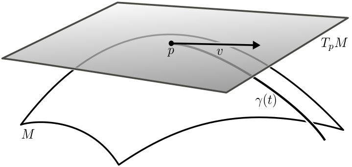
Figure 1. A $2$-manifold $M$ and its tangent space $T_{p}M$ at the point $p$. The geodesic $\gamma(t)$ starts at $p$ in the direction $v$.

Let $p$ be a point in the $3$-manifold $M$, and $\textbf{x}(x_{1},x_{2},x_{3})$ be a parameterization of $M$. The tangent space $T_{p}M$ in $p$ is the vector space generated by the vectors $\{\frac{\partial}{\partial x_{i}}\textbf{x}_{|p}\}$ — the derivatives of the coordinates curves of x at $p$. As $T_{p}M$ admits a linear vector field structure, we can define a scalar product on each tangent space of $M$. If such procedure is “smooth” the result is a metric on $M$.

3.2. Riemannian metric

A Riemannian metric in $M$ is a map $g$ that attributes to each point $p$ a scalar product $\langle\cdot,\cdot\rangle_{p}$ in the tangent space $T_{p}M$, such that in coordinates, $\textbf{x}(x_{1},x_{2},x_{3})=p$, the function $g_{ij}(x_{1},x_{2},x_{3}):=\langle\frac{\partial}{\partial x_{i}},\frac{\partial}{\partial x_{j}}\rangle_{p}$ is smooth. This function does not depend on the coordinate system. We may use $g$ instead of $\langle\cdot,\cdot\rangle$.

Expressing two tangent vectors $u$, $v$, at a point $p\in M$, in terms of the basis $\{\frac{\partial}{\partial x_{i}}(p)\}$, $u=\sum u_{i}\frac{\partial}{\partial x_{i}}(p)$ and $v=\sum v_{i}\frac{\partial}{\partial x_{i}}(p)$, we obtain the scalar product:

(3.1) $$\langle u,v\rangle_{p}=\sum_{i,j=1}^{3}u_{i}v_{j}\langle\frac{\partial}{\partial x_{i}},\frac{\partial}{\partial x_{j}}\rangle(p).$$

The metric tensor $g$ in $M$ is fully determined by the matrix $[g_{ij}]:=[\langle\frac{\partial}{\partial x_{i}},\frac{\partial}{\partial x_{j}}\rangle]$ and generalizes the classical Euclidean inner product of $\mathbb{R}^{3}$. The pair $(M,g)$ is a Riemannian manifold. The chart x bridges $M$ and $\mathbb{R}^{3}$, so that the pull-back of the metric $g$ to $\mathbb{R}^{3}$ results in a Riemannian manifold $(\mathbb{R}^{3},g)$ isometric to $(M,g)$. This work investigates the design and visualization of Riemannian metrics on $\mathbb{R}^{3}$.

3.3. Geodesics

We now investigate the geodesics (rays) in the Riemannian manifold $(M,g)$. In the Euclidean metric, these curves have null acceleration (second derivative). Here, the analogous concept of “acceleration” is defined using the covariant derivative. This is a way to calculate the derivative of tangent fields along curves in manifolds.

A geodesic in a Riemannian manifold $(M,g)$ is a curve $\gamma(t)=(x_{1}(t),x_{2}(t),x_{3}(t))$ with null covariant derivative:

(3.2) $$\small\frac{D}{dt}\gamma^{\prime}=\sum_{k=1}^{3}\left(x^{\prime\prime}_{k}+\sum_{i,j=1}^{n}\Gamma^{k}_{ij}x^{\prime}_{i}x^{\prime}_{j}\right)\frac{\partial}{\partial x^{k}}=0\Longleftrightarrow x^{\prime\prime}_{k}+\sum_{i,j=1}^{3}\Gamma^{k}_{ij}x^{\prime}_{i}x^{\prime}_{j}=0,\,\,k=1,2,3.$$

This differs from the classical by the addition of $\sum\Gamma^{k}_{ij}x^{\prime}_{i}x^{\prime}_{j}$, which includes the Christoffel symbols $\Gamma^{m}_{ij}$ of $(M,g)$.

To linearize System 3.2, we add new variables being the first derivatives $y_{k}=x^{\prime}_{k}$, obtaining thus the geodesic flow of $(M,g)$:

(3.3) $$\left\{\begin{array}[]{ll}x^{\prime}_{k}&=y_{k}\\[0.0pt] y^{\prime}_{k}&=\displaystyle-\sum_{i,j=1}^{n}\Gamma^{k}_{ij}y_{i}y_{j},\,\,\,k=1,2,\ldots,n.\end{array}\right.$$

To compute the geodesic flow in a Riemannian manifold we need its Christoffel symbols at each point. These can be computed in terms of the metric coefficients and its derivatives [4] by the formula:

(3.4) $$\Gamma^{m}_{ij}=\frac{1}{2}\sum_{k=1}^{3}\left(\frac{\partial}{\partial x_{i}}g_{ik}+\frac{\partial}{\partial x_{j}}g_{kj}-\frac{\partial}{\partial x_{k}}g_{ij}\right)g^{km}.$$

Where $[g^{ij}]$ is the inverse matrix of $[g_{ij}]$.

3.4. Exponential map

Let $p$ be a point in $M$ — the observer. A key idea in the ray tracing algorithm is to trace rays from $p$. This is also behind the exponential map: a natural application encoding all the rays leaving $p$:

(3.5) $$\begin{array}[]{llll}\exp_{p}:&T_{p}M&\longrightarrow&M\\ &v&\longmapsto&\gamma(\left\lVert v\right\rVert).\end{array}$$

$\gamma$ is the geodesic satisfying $\gamma(0)=p$ and $\gamma^{\prime}(0)=v$. Intuitively, the exponential map takes a vector $v$ tangent at a point $p$, and runs a geodesic from $p$ towards the direction $v/\left\lVert v\right\rVert$ until the parameter $\left\lVert v\right\rVert$ (see Figure 1).

A natural concern arises: Is $\exp_{p}$ well defined? The well-known Hopf–Rinow theorem [4] gives us an answer. It states that $\exp_{p}$ is defined at the whole tangent space iff the Riemannian manifold is a complete metric space. In our case, $M$ diffeomorphic to $\mathbb{R}^{3}$, then $\exp_{p}$ is defined in the whole space. Additionally, the theorem say that every point in $M$ can be connected to $p$ by a geodesic. Thus, $\exp_{p}$ is surjective implying that every scene in $M$ can be ray traced using this map.

However, $\exp_{p}$ may not be injective: when there exists points in $M$ connected to $p$ by many geodesics. Visualizing such manifolds using rasterization is infeasible.

The Hadamard theorem [4] states that the exponential map will be injective if, additionally, $M$ has non-positive sectional curvature. If we consider $M$ being the paraboloid, given by the graph of $f(x,y,z)=x^{2}+y^{2}+z^{2}$, the exponential map is not injective: there exists pairs of points in $M$ connected by many geodesics.

4. Riemannian shading and illumination

In computer graphics, Shading is the process of assigning a color to a pixel. Classic approaches to perform such tasks are not suited for Riemannian manifolds due to the nonlinear nature of their rays.

Riemannian shading

Consider a viewing $2$-sphere $\mathbb{S}^{2}_{p}$ centered in an observer point $p$ in a $3$-manifold $M$. We give a color for each ray direction in the the observer field $V\subset\mathbb{S}^{2}_{p}$ by tracing a ray; $\mathbb{S}^{2}_{p}\cap V$ carries the image. We call this procedure Riemannian shading. Specifically, the sphere $\mathbb{S}^{2}_{p}$ is centered at the origin of $T_{p}M$. For each direction $v\in V\subset\mathbb{S}^{2}_{p}$, we attribute a color $c$ by launching a ray $\gamma(t)$ from $p$ towards $v$ using the exponential map $exp_{p}$. If $\gamma$ intersects a scene object, we define an RGB color. This is the Riemannian shading $c:\mathbb{S}^{2}_{p}\to\mathcal{C}$, where $\mathcal{C}$ is a color space.

Riemannian illumination

The Riemannian illumination of a point $q$ in an embedded surface $S\subset M$ comes from direct geodesics connecting $q$ to the light sources and indirect geodesics connecting other Riemannian-illuminated points to $q$. The radiant intensity at $q$ is modeled using the Lambertian reflectance, which depends on the Riemannian metric, or more generally from a BRDF. For a point $p$ in $M$, we compute the Riemannian shading using ray tracing and Riemannian illumination.

Classical ray tracing [9] approximates physical illumination. Our Riemannian ray tracing model can be also used to compute a Riemannian shading function for local or global illumination. This work uses pseudo-color based on properties of the space, such as a coordinated point, to define the Riemannian shading function.

4.1. Ray Marching

To launch a ray we need to solve the geodesic flow (Eq 3.3) and subsequently compute the intersection of the given ray with the scene objects. In general, our rays will be curved and are solutions of the geodesic flow which we have resorted to numerical integration methods.

We use Euler’s method for integration in the parameterization image, since there we use the Euclidean metric. The Euler’s numerical integration method approximates a ray $\gamma$ starting at $p$ in the direction $v$ by a polygonal $\{p_{i}\}$:

(4.1) $$\left\{\begin{array}[]{l}p_{i+1}=p_{i}+h\cdot\widetilde{\gamma}^{\prime}(0)\\ v_{i+1}=v_{i}+h\cdot\widetilde{\gamma}^{\prime\prime}(0)\end{array}\right.$$

where $h$ is the integration step and $\widetilde{\gamma}(t)$ is the ray satisfying $\widetilde{\gamma}(0)=p_{i}$ and $\widetilde{\gamma}^{\prime}(0)=v_{i}$. We use Equation 3.3 to compute $\widetilde{\gamma}^{\prime\prime}(0)$.

The polygonal $\{p_{i}\}$ is used to ray trace a scene in $(M,g)$. When $h\to\epsilon$ the scene is accurately rendered. For the ray-scene intersection, we check the for each segment given by the polygonal approximation given by Equation 4.1 (i.e., ray marching).

For now, we are testing the intersection with each segment sequentially. In future works, we pretend to use many segments of the polygonal $\{p_{i}\}$ to increase the GPU occupancy and optimize the intersection computations. This idea was suggested by Ingo Wald during GTC 2020.

We could use the Runge–Kutta method to approximate solutions of the geodesic flow. Instead, we consider the Euler method since it uses fewer computations giving GPU performance.

5. Examples of Riemannian metrics

This section presents two examples of Riemannian metrics in $\mathbb{R}^{3}$. The first is given by pushing the metric from the graph of three-dimensional functions, the other comes from deformations of $\mathbb{R}^{3}$ given by diffeomorphisms.

5.1. Graph of a function

Let $f:\mathbb{R}^{3}\to\mathbb{R}$ be a smooth function. We construct a Riemannian metric $g$ in $\mathbb{R}^{3}$ which is the pullback of the metric of the graph of $f$:

$$M_{f}=\{(x_{1},x_{2},x_{3},x_{4})\in\mathbb{R}^{4}|\,\,f(x_{1},x_{2},x_{3})=x_{4}\}.$$

$M_{f}$ is parameterized in the obvious way by $\textbf{x}(x_{1},x_{2},x_{3})=(x_{1},x_{2},x_{3},f(x_{1},x_{2},x_{3}))$. The tangent space $T_{p}M_{f}$ at a point $p$ is generated by the vectors:

(5.1) $$\frac{\partial}{\partial x_{i}}(p)=(e_{i},f_{i}(p)).$$

Where $f_{i}(p)$ is the partial derivative of $f$ in the standard direction $e_{i}$. We use the Euclidean metric of $\mathbb{R}^{4}$ to induce a Riemannian metric $g$ in $M_{f}$.

Let $p$ be a point in $M_{f}$, we compute the metric $g$ at $p$. Replacing the expression of Equation 5.1 in $\langle\frac{\partial}{\partial x_{i}},\frac{\partial}{\partial x_{j}}\rangle$, we obtain the coefficients of the Riemannian metric:

(5.2) $$g_{ii}=1+f_{i}^{2}\,\,\mbox{and }g_{ij}=f_{i}f_{j},\,\,\mbox{ if }i\neq j,$$

which are smooth functions of $M_{f}$, then $g$ is Riemannian. In terms of measure, the metric $g$ makes the volume vary beautifully because its volume formula, used to compute integrals in $(M_{f},g)$, has the form $\det[g_{ij}]=1+\left\lVert\nabla f\right\rVert^{2}$. Then, it only matches with the standard if $\nabla f=0$.

We present the geodesics of $(M_{f},g)$. A direct calculation using the software Maple implies in $g^{ii}=\frac{f_{j}+f_{k}}{1+\left\lVert\nabla f\right\rVert^{2}}$, with $i$, $j$, $k$ being all distinct, and $g^{ij}=-\frac{f_{i}f_{j}}{1+\left\lVert\nabla f\right\rVert^{2}}$, if $i\neq j$. Substituting these in Equation 3.4, and using software Maple, we obtain a simple formula for the Christoffel symbols of $(M_{f},g)$:

(5.3) $$\Gamma^{m}_{ij}=\frac{f_{m}f_{ij}}{1+\left\lVert\nabla f\right\rVert^{2}}.$$

Where $f_{ij}$ is the second order partial derivative in the direction $e_{i}$, and $e_{j}$. Replacing the Christoffel symbols of $M_{f}$ in this Equation 3.4 we obtain.

(5.4) $$\left\{\begin{array}[]{ll}x^{\prime}_{k}&=y_{k}\\ y^{\prime}_{k}&=\displaystyle-\sum_{i,j=1}^{3}\frac{f_{k}f_{ij}}{1+\left\lVert\nabla f\right\rVert^{2}}y_{i}y_{j},\,\,\,k=1,2,3.\end{array}\right.$$

For a concrete example, consider $M_{f}$ being the graph of the polynomial function $f(x,y,z)=x^{2}+y^{2}-z^{2}$. The Christoffel symbols of this parameterization are computed using Equation 5.3. Replacing the result in Equation 5.4 we obtain a geodesic flow. Figure 2 gives an inside view of the space $\mathbb{R}^{3}$ endowed with the geometry pulled back from $M_{f}$ by the parameterization $\Phi(x,y,z)=(x,y,z,f(x,y,z))$. In the left image, we positioned the camera looking towards direction $x$. On the right image, the camera points at the direction $z$. The scene is composed of a regular grid in $\mathbb{R}^{3}$ distorted by $\Phi$.

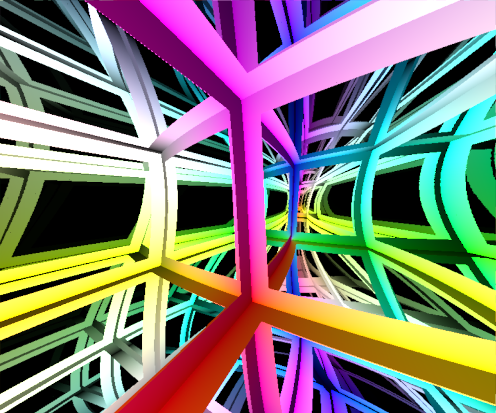
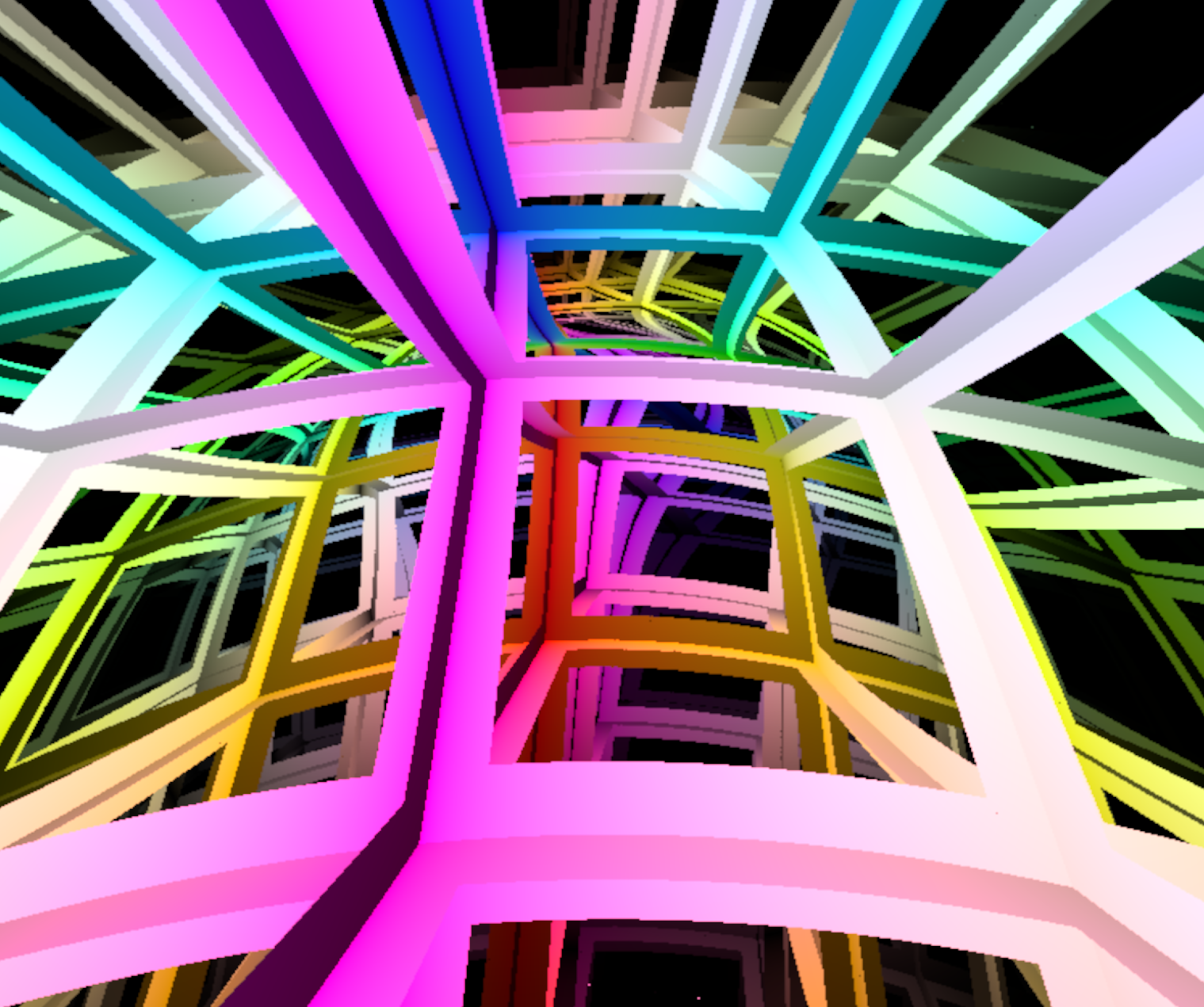
Figure 2. The space $\mathbb{R}^{3}$ endowed with the geometry of the graph of the function $f(x,y,z)=x^{2}+y^{2}-z^{2}$. On the left, a look towards direction $x$. On the right, a look in the direction $z$.

5.2. Diffeomorphisms

Let $\Phi:\mathbb{R}^{3}\to\mathbb{R}^{3}$, given by $\Phi(p)=(x_{1}(p),x_{2}(p),x_{3}(p))$, be a diffeomorphism. We put a metric in $\mathbb{R}^{3}$ based in the deformations provided by $\Phi$. Our base manifold in this case is $\mathbb{R}^{3}$ parameterized by $\Phi$, and its associated base is given by:

(5.5) $$\frac{\partial}{\partial x_{i}}=(\frac{\partial}{\partial x_{i}}x_{1},\frac{\partial}{\partial x_{i}}x_{2},\frac{\partial}{\partial x_{i}}x_{3}).$$

We pullback the Euclidean metric of $\mathbb{R}^{3}$ through the differential of $\Phi$, this will provide a new metric $g$ on $\mathbb{R}^{3}$.

The metric $g$ at a point $p\in\mathbb{R}^{3}$ is completely determined by the metric tensor $[g_{ij}]:=[\langle\frac{\partial}{\partial x_{i}},\frac{\partial}{\partial x_{j}}\rangle]$. Thus subtituing Equation 5.5 in $\langle\frac{\partial}{\partial x_{i}},\frac{\partial}{\partial x_{j}}\rangle$, we obtain the following formula:

(5.6) $$g_{ij}=\displaystyle\sum_{k=1}^{3}\frac{\partial}{\partial x_{i}}x_{k}\frac{\partial}{\partial x_{j}}x_{k}.$$

As $g_{ij}$ are smooth functions, $g$ is Riemannian.

We now compute the geodesics of $(\mathbb{R}^{3},g)$. By Equation 3.2 we must first calculate the Christoffel symbols. Replacing the metric in Equation 5.6 in Christoffel symbols Equation 3.4 and using software Maple, we obtain a simple formula:

$$\Gamma^{m}_{ij}=\sum_{s=1}^{3}\left(\frac{\partial^{2}}{\partial x_{i}\partial x_{j}}x_{s}\cdot(-1)^{s+m}\cdot\frac{\det J_{sm}}{\det J}\right).$$

Where $J$ is the Jacobian matrix of $\Phi$, and $J_{sm}$ is $J$ without the $s$-line and the $m$-column: the $(s,m)$-minor of $J$. The term $(-1)^{s+m}\cdot\frac{\det J_{sm}}{\det J}$ in the equation is the $(m,s)$-coefficient of the inverse of $J$. Thus we obtain a beautiful formula.

Theorem 5.1.

Let $\Phi(p)=(x_{1}(p),x_{2}(p),x_{3}(p))$ be a diffeomorphism of $\mathbb{R}^{3}$. Then, the Christoffel symbols of $\Phi$ are given by:

(5.7) $$\Gamma^{m}_{ij}=\sum_{s=1}^{3}\left(\frac{\partial^{2}}{\partial x_{i}\partial x_{j}}x_{s}\cdot[J^{-1}]_{ms}\right).$$

Theorem 5.1 says that the Christoffel symbols of $(\mathbb{R}^{3},g)$ can be computed using only the Jacobian and Hessian operators of the parameterization $\Phi$. For the best of our knowledge, this is the first time such a formula appears. Equation 5.7 will be very useful when the parameterization $\Phi$ be a composition of parameterizations.

Replacing the Christoffel symbols in the Eq. 3.2, we obtain its geodesic flow:

(5.8) $$\left\{\begin{array}[]{ll}x^{\prime}_{k}&=y_{k}\\ y^{\prime}_{k}&=\displaystyle-\sum_{i,j,s=1}^{3}\left(\frac{\partial^{2}}{\partial x_{i}\partial x_{j}}x_{s}\cdot[J^{-1}]_{ms}\right)y_{i}y_{j},\,\,\,k=1,2,3.\end{array}\right.$$

For an explicit example of a deformation of $\mathbb{R}^{3}$, we consider the following twist map

$$\Phi(x,y,z)=(\cos(z)x-\sin(z)y,\sin(z)x+\cos(z)y,z).$$

The Christoffel symbols of this parameterization are computed using Equation 5.7. Replacing the result in Equation 5.8 we obtain a geodesic flow. We give an inside view of this “twisted” $\mathbb{R}^{3}$ by tracing rays using Riemannian shading. Figure 3 shows an immersive view of a regular grid in $\mathbb{R}^{3}$ distorted by $\Phi$.

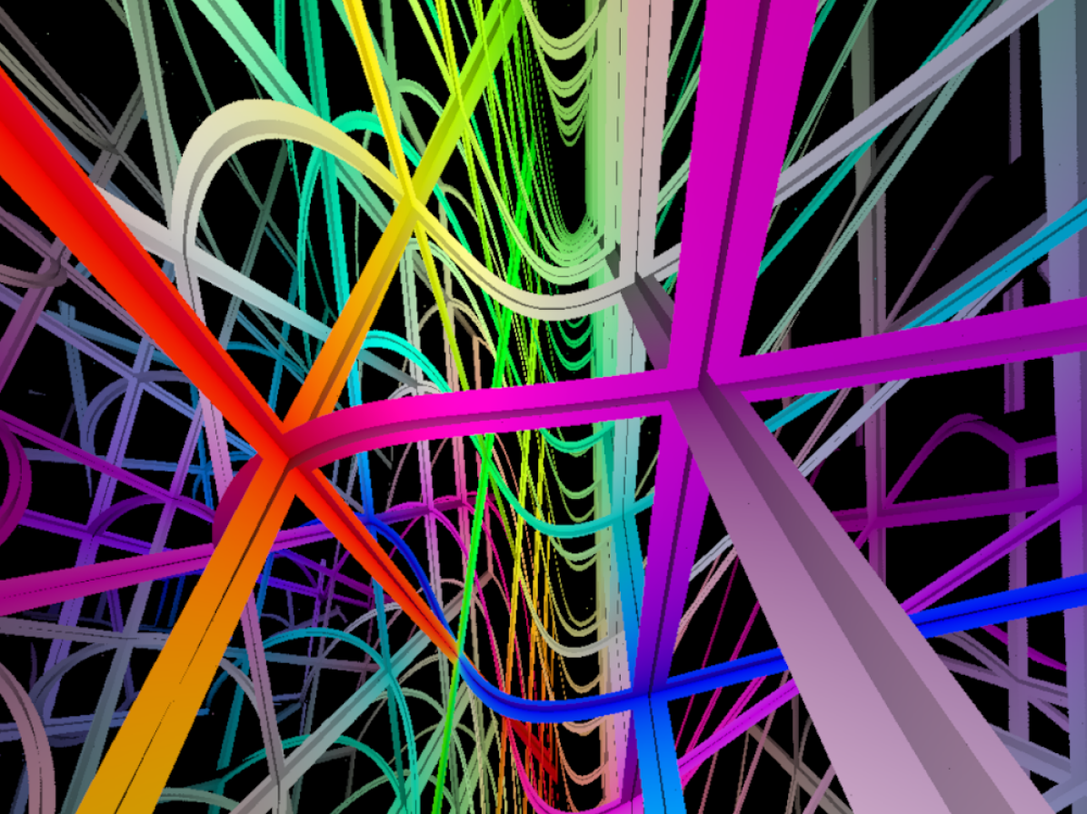
Figure 3. The space $\mathbb{R}^{3}$ deformed using a “twist” along the planes perpendicular to the $z$-axis. The RGB colors are given by the $(x,y,z)$ coordinates of the hit points.

6. Deforming the space

This section describes two convenient ways of accumulating local deformations of $\mathbb{R}^{3}$. The first is an extension of Subsection 5.1 consisting of summing functions. The second deals with the composition of deformations. In both cases, the functions and deformations are modeled using Gaussians. Many techniques in Computer Graphics depends on these functions due to their flexibility in modeling and smoothness.

6.1. Local metric deformations

We model graphs and deformations using the three-dimensional Gaussian function

(6.1) $$f(x,y,z)=a\cdot\exp\left(-\frac{(x-x_{0})^{2}}{2\sigma_{x}^{2}}-\frac{(y-y_{0})^{2}}{2\sigma_{y}^{2}}-\frac{(z-z_{0})^{2}}{2\sigma_{z}^{2}}\right).$$

Where $a$ is the amplitude, $(x_{0},y_{0},z_{0})$ is the center, and $\sigma_{x}$, $\sigma_{y}$, $\sigma_{z}$ are the spreads.

Using graphs

Using Subsection 5.1, we visualize the graph $M_{f}=\{p\in\mathbb{R}^{4}|z=f(x,y,z)\}$. Figure 4 shows inside views of $M_{f}$ by varying the parameters of $f$. The first image presents the case of zero amplitude. The second image illustrates a small deformation given by a small amplitude and spreads values. The third and fourth images have small amplitude with lager spreads, and vice-versa. In all the cases, the scene is composed of a regular grid and the ray tracing has a small (black) fog component. This is why in the fourth image there is a black region in the center of the deformation.

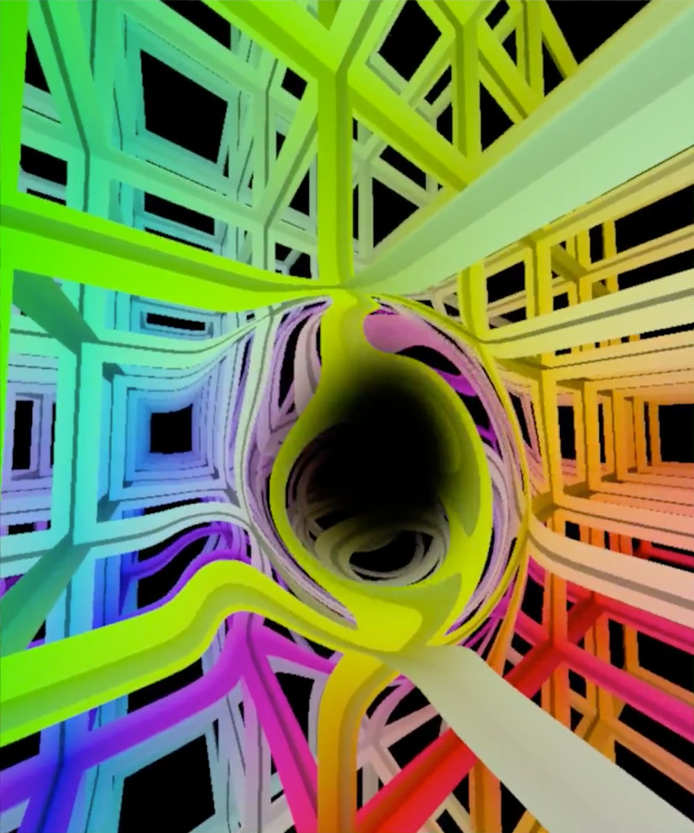
Figure 4. The space $\mathbb{R}^{3}$ endowed with no deformation, local deformation, and global deformation.

Using diffeomorphism

We present a formula to deform a neighborhood of a point $q$ in $\mathbb{R}^{3}$. Consider a Gaussian function $f$ centered at $q$, choosing small spreads values for $f$, the formula

(6.2) $$\Phi(p)=p+f(p)\cdot v$$

deforms the neighborhood of $q$ at the direction $v$.

For a more refined formula, replace $v$ by a vector field $V$. The resulted formula $\Phi(p)=p+f(p)\cdot V(p)$ deforms a neighborhood of $q$ following the instructions of $V$.

6.2. Accumulating deformations

We present two ways of accumulating deformations: summing the functions or the deformations presented above, and composing diffeomorphism.

Summing functions

Let $f_{1},f_{2},\ldots,f_{k}$ be functions taking values in $\mathbb{R}^{3}$. The graph of the function $f=f_{1}+f_{2}+\ldots+f_{k}$ is given by

$$M_{f}=\{p\in\mathbb{R}^{4}|(f_{1}+f_{2}+\ldots+f_{k})(x_{1},x_{2},x_{3})=x_{4}\}.$$

As we saw in Subsection 5.1, the manifold $M_{f}$ endows the metric of $\mathbb{R}^{4}$. Equation 5.2 says that this metric is given by $g_{ij}=1+\left(\frac{\partial f}{\partial x_{i}}\right)^{2}$ and $g_{ij}=\frac{\partial f}{\partial x_{i}}\frac{\partial f}{\partial x_{j}}$ if $i\neq j$. Then the metric $[g_{ij}]$ is easily computed because

$$\frac{\partial f}{\partial x_{i}}=\frac{\partial(f_{1}+f_{2}+\ldots+f_{k})}{\partial x_{i}}=\frac{\partial f_{1}}{\partial x_{i}}+\frac{\partial f_{2}}{\partial x_{i}}+\ldots+\frac{\partial f_{k}}{\partial x_{i}}.$$

In other words, to compute the metric $g$ we only need to store the partial derivatives of each function $f_{i}$. The pair $(M_{f},g)$ is the desired Riemannian manifold.

We now compute the geodesic flow of $(M_{f},g)$. The geodesic Equation 3.2 is given by the Christoffel symbols of $(M_{f},g)$, which are presented as $\Gamma^{m}_{ij}=\frac{f_{m}f_{ij}}{1+\left\lVert\nabla f\right\rVert^{2}}$ by Eq. 5.3 in terms of $f$. Therefore, the symbols $\Gamma^{m}_{ij}$ can be computed using the first and second partial derivatives of the functions $f_{i}$’s.

To show the effects in visualizing graphs of summed functions, consider a regular grid embedded in $\mathbb{R}^{3}$ (Left image in Figure 5). Adding a unique Gaussian function in the summation (middle image in Figure 5). Summing two Gaussian functions (right image in Figure 5).

Figure 5. Space $\mathbb{R}^{3}$ endowed with no deformation, one local deformation, and two local deformations.

Composing diffeomorphisms

Let $\Phi_{1},\Phi_{2},\ldots,\Phi_{k}$ be a sequence of diffeomorphisms of $\mathbb{R}^{3}$, we pretend to compute the Riemannian metric $g$ on $\mathbb{R}^{3}$ that carries the deformations of the composition $\Phi=\Phi_{1}\circ\Phi_{2}\circ\ldots\circ\Phi_{k}$. Then we derive the geodesic flow of the resulting Riemannian manifold $(\mathbb{R}^{3},g)$ for a possible ray tracing.

Equation 5.6 states that the metric $g$ is given by $g_{ij}=\sum_{k}\frac{\partial}{\partial x_{i}}x_{k}\frac{\partial}{\partial x_{j}}x_{k}$, where $\Phi(p)=(x_{1}(p),x_{2}(p),x_{3}(p))$. In other words, to compute the metric coefficients $g_{ij}$, we only need the Jacobian matrix $J(\Phi)$ of $\Phi$ which is easily obtained using the chain rule formula $J(\Phi)=J(\Phi_{1})\cdot J(\Phi_{2})\cdot\ldots\cdot J(\Phi_{k})$.

To compute the geodesic flow of the Riemannian manifold $(\mathbb{R}^{3},g)$, we need its Christoffel symbols, which are provided by the Jacobian $J(\Phi)$ and the Hessian $H(\Phi)$ operator of $\Phi$ (from Theorem 5.1) using the formula $\Gamma^{m}_{ij}=\sum_{s}\left(\frac{\partial^{2}}{\partial x_{i}\partial x_{j}}x_{s}\cdot[J^{-1}]_{ms}\right)$. Specifically, to compute $\Gamma^{m}_{ij}$, we invert the Jacobian $J(\Phi)$ of $\Phi$ using the formula

$$J^{-1}(\Phi)=J^{-1}(\Phi_{k})\cdot J^{-1}(\Phi_{k-1})\cdot\ldots\cdot J^{-1}(\Phi_{1}).$$

It is not direct to compute the Hessian component $\frac{\partial^{2}}{\partial x_{i}\partial x_{j}}x_{s}$ of $\Phi$, where $x_{s}(p)$ is the $s$-coordinate of $\Phi(p)$. Firstly, we consider the composition of only two diffeomorphisms $\Phi=\Phi_{1}\circ\Phi_{2}$, then we extend it to the composition of diffeomorphisms.

The Hessian matrix of the coordinate of $\Phi=\Phi_{1}\circ\Phi_{2}=(x_{1}\circ\Phi_{2},x_{2}\circ\Phi_{2},x_{3}\circ\Phi_{2})$, that is $H(x_{s}\circ\Phi_{2})$, is given by

(6.3) $$H(x_{s}\circ\Phi_{2})_{p}=J^{T}(\Phi_{2})_{p}\cdot H(x_{s})_{\Phi_{2}(p)}\cdot J(\Phi_{2})_{p}+\nabla x_{s}(\Phi_{2}(p))\cdot H(\Phi_{2})_{p}$$

We extended Equation 6.3 to $x_{s}\circ\Phi_{2}\circ\Phi_{3}$, that is, we consider the composition of three diffeomorphisms $\Phi=\Phi_{1}\circ\Phi_{2}\circ\Phi_{3}$. For this, we apply Equation 6.3 to $H((x_{s}\circ\Phi_{2})\circ\Phi_{3})_{p}$, then after some computations we obtain:

$$\begin{array}[]{lll}H(x_{s}\circ\Phi_{2}\circ\Phi_{3})_{p}&=&J^{T}(\Phi_{2}\circ\Phi_{3})_{p}\cdot H(x_{s})_{\Phi_{2}\circ\Phi_{3}(p)}\cdot J(\Phi_{2}\circ\Phi_{3})_{p}\\ &+&J^{T}(\Phi_{3})_{p}\cdot\nabla x_{s}(\Phi_{2}\circ\Phi_{3}(p))\cdot H(\Phi_{2})_{\Phi_{3}(p)}\cdot J(\Phi_{3})_{p}\\ &+&\nabla(x_{s}\circ\Phi_{2})(\Phi_{3}(p))\cdot H(\Phi_{3})_{p}\end{array}$$

The general formula is obtained through an inductive argument. We simplify the notation by considering $\Phi_{[i,j]}:=\Phi_{i}\circ\ldots\circ\Phi_{j}$, for each $i<j$. Therefore

$$H(x_{s}\circ\Phi_{[2,k]})_{p} =J^{T}(\Phi_{[2,k]})_{p}\cdot H(x_{s})_{\Phi_{[2,k]}(p)}\cdot J(\Phi_{[2,k]})_{p}$$

$$+\displaystyle\sum_{i=3}^{k}J^{T}(\Phi_{[i,k]})_{p}\cdot\nabla(x_{s}\circ\Phi_{[2,i-2]})(\Phi_{[i-1,k]}(p))\cdot H(\Phi_{i-1})_{\Phi_{[i,k]}(p)}\cdot J(\Phi_{[i,k]})_{p}$$

$$+\nabla(x_{s}\circ\Phi_{[2,k-1]})(\Phi_{k}(p))\cdot H(\Phi_{k})_{p}$$

From a computational point of view, this is an important formula because it computes $H(x_{s}\circ\Phi_{[2,k]})_{p}$ in terms of the Jacobians and Hessians of each diffeomorphism $\Phi_{i}$ separately. Therefore, during the computations only the partial derivatives of each diffeomorphism must be stored, the partial derivatives of the compositions are derived from them.

References

- [1] Riemannian ray tracing, 2019.
- [2] Alan H Barr, Ray tracing deformed surfaces, ACM SIGGRAPH Computer Graphics 20 (1986), no. 4, 287–296.
- [3] Pierre Berger, Alex Laier, and Luiz Velho, An image-space algorithm for immersive views in 3-manifolds and orbifolds, Visual Computer (2014).
- [4] Manfredo Perdigao do Carmo, Riemannian geometry, Birkhäuser, 1992.
- [5] Eduard Gröller, Nonlinear ray tracing: Visualizing strange worlds, The Visual Computer 11 (1995), no. 5, 263–274.
- [6] Tiago Novello, Vinicius da Silva, and Luiz Velho, Visualization of nil, sol, and sl2 geometries, In preparation, IMPA, 2020.
- [7] Jos Stam and Eric Languénou, Ray tracing in non-constant media, Rendering Techniques’ 96, Springer, 1996, pp. 225–234.
- [8] Luiz Velho, Vinicius da Silva, and Tiago Novello, Immersive visualization of the classical non-euclidean spaces using real-time ray tracing in vr, In Proceedings of the 46th Graphics Interface, 2020.
- [9] Turner Whitted, An improved illumination model for shaded display, ACM SIGGRAPH Computer Graphics, vol. 13, ACM, 1979, p. 14.