Stability of clusters in the second–order Kuramoto model on random graphs

Abstract

The Kuramoto model of coupled phase oscillators with inertia on Erdős-Rényi graphs is analyzed in this work. For a system with intrinsic frequencies sampled from a bimodal distribution we identify a variety of two cluster patterns and study their stability. To this end, we decompose the description of the cluster dynamics into two systems: one governing the (macro) dynamics of the centers of mass of the two clusters and the second governing the (micro) dynamics of individual oscillators inside each cluster. The former is a low-dimensional ODE whereas the latter is a system of two coupled Vlasov PDEs. Stability of the cluster dynamics depends on the stability of the low-dimensional group motion and on coherence of the oscillators in each group. We show that the loss of coherence in one of the clusters leads to the loss of stability of a two-cluster state and to formation of chimera states. The analysis of this paper can be generalized to cover states with more than two clusters and to coupled systems on W-random graphs. Our results apply to a model of a power grid with fluctuating sources.

1 Introduction

Understanding principles underlying collective behavior in large networks of interacting dynamical systems is an important problem with applications ranging from neuronal networks to power grids. Many dynamical models on networks have been proposed to this effect. The Kuramoto model (KM) of coupled phase oscillators has had a widespread success due to its analytical simplicity and universality of the dynamical mechanisms that it helped to reveal. It describes the evolution of interconnected phase oscillators $u_{n,i}:{\mathbb{R}}^{+}\to{\mathbb{R}}/2\pi{\mathbb{Z}}$ having intrinsic frequencies $\omega_{n,i}$:

$$\dot{u}_{n,i}=\omega_{n,i}+Kn^{-1}\sum_{j=1}^{n}a_{n,ij}\sin\left(u_{n,j}-u_{n,i}+\alpha\right),\quad i\in[n].$$ (1.1)

The sum on the right–hand side models the interactions between the oscillators, $\alpha\in[0,2\pi)$ determines the type of interactions (attractive vs repulsive), and $K$ is the strength of coupling. The spatial structure of interconnections is encoded in the adjacency matrix $(a_{n,ij})$. The KM plays an important role in the theory of synchronization. We mention two major contributions that are especially relevant to the present study. First, it reveals a universal mechanism for the transition to synchronization in systems of coupled oscillators with random intrinsic frequencies. The analysis of the KM shows that there is a critical value of the coupling strength $K_{c}$ separating the incoherent (mixing) dynamics (Fig. 1a) from synchronization (Fig. 1b) [19, 7, 8]. Second, studies of the KM led to the discovery of chimera states, patterns combining regions of coherent and incoherent dynamics [11, 1, 15].

Having reviewed the classical KM, we now turn to its generalization that is the main focus of this paper:

$$\ddot{u}_{n,i}+\gamma\dot{u}_{n,i}=\omega_{n,i}+Kn^{-1}\sum_{j=1}^{n}a_{n,ij}\sin\left(u_{n,j}-u_{n,i}+\alpha\right),\quad i\in[n].$$ (1.2)

The main new additions here are the second-order terms. The other parameters are the damping constant $\gamma>0$ and the random torques $\omega_{n,i}$, which we keep referring to as intrinsic frequencies to emphasize the parallels with the classical KM (1.1). The system of equations (1.2) can be viewed a model of coupled pendula. Systems of equations like (1.2) are widely used for modeling power networks [9, 18]. The inclusion of the second order terms makes the dynamics substantially more complex [3, 20, 10]. In particular, the second order model is known for its capacity to generate a rich variety of coherent clusters [20, 5]. Clusters exist for different types of connectivity and different probability distributions of intrinsic frequencies. We experimented with uniform, Gaussian, and certain multimodal distributions and used all-to-all and random Erdős-Rényi (ER) connectivity. In each case, we saw an abundance of clusters (Fig. 2). Furthermore, we often found multiple cluster states coexisting for the same values of parameters (Fig. 3).

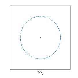
a)  b)

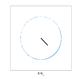
Fig.  1: The distribution of the oscillators in the phase space is shown for a) $K<K_{c}$ and for b) $K>K_{c}$. The complex order parameter is plotted as a black arrow. It points to the center of mass of the coherence buildup.

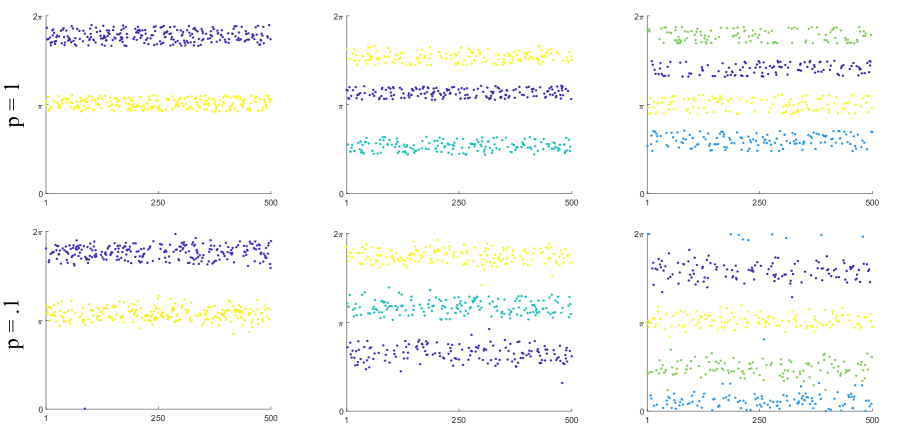
Fig.  2: The snapshots of coexisting distinct stable clusters in (1.2). The intrinsic frequencies are chosen uniformly from $[-2,2]$. The values of other parameters are $K=3$ and $\gamma=.1$. The plots in the top line are made for the model on complete graphs and those in the bottom line - for that on an ER graph with $p=.1$. Oscillators are color coded by instantaneous velocity to reveal clustering. By choosing carefully initial conditions for the two models, one can generate $2-,3-,4-$ and other cluster states.

Determining stability of clusters is a challenging problem. For the second order KM with identical oscillators it has been studied [5], where the problem was reduced to the analysis of the damped pendulum equation. For the model with random intrinsic frequencies and random network topologies, linear stability of synchronization was studied in [21]. For the model with random intrinsic frequencies, stability of clusters has not been studied before. We show that this is a multiscale problem. At a microscopic level, the formation of clusters requires a mechanism by which the oscillators within a cluster stay coherent, i.e., synchronization within a cluster. On the other hand, clusters have nontrivial (macroscopic) dynamics of their own. Thus, in addition to synchronization, the stability of clusters depends on the stability of the macroscopic group motion.

In this paper, we study stability of clusters in the model with random intrinsic frequencies and ER random connectivity. We restrict to two-cluster states and assume a bimodal distribution of intrinsic frequencies. These assumptions are made to simplify the presentation. The same approach can be used for studying patterns with three and more groups of coherent oscillators. Likewise, the multimodality of the intrinsic frequency distribution is not necessary for cluster formation. The same mechanism is responsible for the formation of clusters when intrinsic frequencies are distributed uniformly (see Fig. 2). However, in this case additional care is needed to identify the clusters analytically. We do not address this issue in this paper. Furthermore, the same formalism applies to the KM on other random graphs [12]. We develop a general framework for studying clusters in large systems of coupled phase oscillators with randomly distributed parameters. As in [5], we write down a low-dimensional system describing the macroscopic (group) dynamics of clusters. Further, we derive a system of kinetic PDEs characterizing the stochastic dynamics of fluctuations with each cluster. The PDE for each cluster incorporates the information about the group motion as well as the fluctuations in other clusters. The low–dimensional equation for the group dynamics and the system of PDEs for fluctuations contain all information determining the stability of clusters. The former system can be further reduced to the equation of damped pendulum and analyzed using standard methods of the qualitative theory of ordinary differential equations [2]. On the other hand, the analysis of the two coupled Vlasov equations is a hard problem, which we do not pursue in general. Instead, we focus on parameter regimes when the two PDEs decouple, which simplifies the analysis. The stability analysis in these parameter regimes suggests a scenario for the loss of stability of a two-cluster state due to the loss of coherence in one of the clusters. Specifically, we show that decoupling of the system of Vlasov equations results in the fluctuations in one cluster being practically independent from the fluctuations in the other cluster. Thus, by controlling the fluctuations in one of the clusters we can make it incoherent, while keeping the other cluster coherent. This provides a new scenario of the loss of stability of a two-cluster state leading to the creation of a chimera state.

The outline of the paper is as follows. In Section 2, we develop a macro-micro decomposition of the cluster dynamics into a low dimensional (group) motion of the centers of mass of two clusters and the system of equations governing the fluctuations in each group. For the latter system, we derive a system of two Vlasov PDEs describing the probability densities for the fluctuations in the limit as the number of oscillators in each cluster tends to infinity. The macro-micro decomposition of the cluster dynamics is the main tool and the main contribution of this paper. In Section 3, we review the key facts about the dynamics of a damped pendulum [2] that will be needed below. In Section 4, we turn to the analysis of fluctuations. We identify two parameter regimes when the two Vlasov equations decouple and the coherence in each cluster can be analyzed separately. We use linear stability analysis of the incoherent state in the KM with inertia [6], to locate the critical values for the loss of coherence in each cluster. Then we identify parameters where oscillators in one cluster lose coherence, while the oscillators in the other cluster remain synchronized. This leads to formation of chimera states. We illustrate this scenario with numerical experiments. Numerics are consistent with the theoretical predictions. We conclude with a brief discussion of the main results in Section 5.

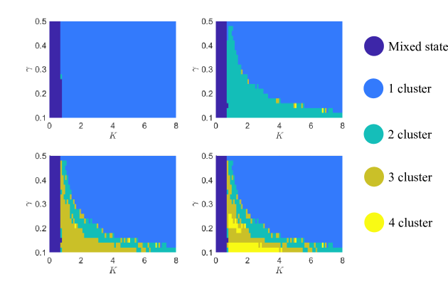
Fig.  3: Regions of existence of stable $d$-cluster states shown for for $d=1$, $1\leq d\leq 2$, $1\leq d\leq 3$ and $1\leq d\leq 4$ superimposed on each other. The diagrams show a substantial region in the parameter space with coexisting stable $1-$, $2-$, $3-$, and $4-$cluster states. The frequencies are sampled from the uniform distribution on $[-.5,.5].$

2 The macro-micro decomposition

2.1 The model

For simplicity, we restrict our study to a two–cluster case. To this end, we assume a bimodal distribution for $\omega_{n,i}$’s. Specifically, we assume that there are two groups of oscillators $u_{1},u_{2},\dots,u_{m}$ and $u_{m+1},u_{m+1},\dots,u_{m+l},$ $n=m+l$. The intrinsic frequencies assigned to the oscillators in the first and second groups are taken from probability distributions with densities $\tilde{g}_{1}(\omega)$ and $\tilde{g}_{2}(\omega)$ respectively. Denote the first two central moments by

$$\bar{\omega}_{1}=\int\omega\tilde{g}_{1}(\omega)d\omega,\;\bar{\omega}_{2}=\int\omega\tilde{g}_{2}(\omega)d\omega,\;\sigma_{1}^{2}=\int(\omega-\bar{\omega}_{1})^{2}\tilde{g}_{1}(\omega)d\omega,\;\sigma_{2}^{2}=\int(\omega-\bar{\omega}_{1})^{2}\tilde{g}_{1}(\omega)d\omega.$$ (2.1)

We assume

$$\delta=\bar{\omega}_{2}-\bar{\omega}_{1}>0,\quad 0<\sigma_{1}^{2},\sigma_{2}^{2}\ll\delta,$$ (2.2)

and $g_{1,2}(y)=\tilde{g}_{1,2}(\bar{\omega}_{1,2}+y)$ are even unimodal functions. Further, we assume that the initial positions and velocities for each cluster $\{u_{n,k}(0)\}_{k=1}^{m},$ $\{\dot{u}_{n,k}(0)\}_{k=1}^{m},$ $\{u_{n,m+k}(0)\}_{k=1}^{l},$ $\{\dot{u}_{n,m+k}(0)\}_{k=1}^{l}$, are sequences of independent identically distributed (each sequence has its own distribution in general) random variables, which satisfy assumptions of the Strong Law of Large Numbers.

In addition, we assume that the underlying network has sparse ER connectivity:

$${\mathbb{P}~{}}(a_{n,ij}=1)=p_{n},$$ (2.3)

where $(p_{n})$ is a positive nonincreasing sequence that is either $p_{n}\equiv p\in[0,1]$ or $p_{n}\searrow 0$ such that $p_{n}n\to\infty$ as $n\to\infty$. In the latter case, we obtain a sequence of sparse ER graphs of unbounded degree. Thus, below we study the following system of ODEs:

$$\ddot{u}_{n,i}+\gamma\dot{u}_{n,i}=\omega_{n,i}+K(p_{n}n)^{-1}\sum_{j=1}^{n}a_{n,ij}\sin\left(u_{n,j}-u_{n,i}+\alpha\right),\quad i\in[n].$$ (2.4)

The analysis of this can be easily generalized to a more general W-random graph model (cf.  [12]). We restrict to the ER case to keep the notation simple.

2.2 The group dynamics

In this and the following subsections, we decompose the dynamics of clusters into two systems: one governing the macroscopic dynamics of individual clusters and the second governing the microscopic dynamics of individual particles inside each cluster. The former is a system of low dimensional ODEs and the latter is a system of PDEs of Vlasov type.

Denote

$$U_{n,1}=m^{-1}\sum_{k=1}^{m}u_{n,k},\;U_{n,2}=l^{-1}\sum_{k=1}^{l}u_{n,m+k},$$ (2.5)

where

$$\begin{array}[]{ll}v_{n,i}=u_{n,i}-U_{n,1},&\quad i\in[m],\\ v_{n,m+j}=u_{n,m+j}-U_{n,2},&\quad j\in[l].\end{array}$$ (2.6)

We assume that the dynamics in each cluster are (predominantly) coherent:

$$\max_{i\in[n]}|v_{i}|\leq\varepsilon\ll 1.$$ (2.7)

Adding up the first $m$ equations in (1.1) and dividing by $m$, we have

$$\begin{split}\ddot{U}_{n,1}+\gamma\dot{U}_{n,1}=&\bar{\omega}_{n,1}+{K\over mnp_{n}}\sum_{i=1}^{m}\sum_{j=1}^{m}a_{n,ij}\sin\left(v_{n,j}-v_{n,i}\right)\\ +&{K\over mnp_{n}}\sum_{i=1}^{m}\sum_{j=1}^{l}a_{n,ij}\sin\left(U_{n,2}-U_{n,1}+[v_{n,m+j}-v_{n,i}]+\alpha\right).\end{split}$$ (2.8)

Rewrite the last sum on the right–hand side of (2.8) as

$$\begin{split}\sum_{i=1}^{m}\sum_{j=1}^{l}a_{n,ij}\sin\left(U_{n,2}-U_{n,1}-\alpha+v_{n,m+j}-v_{n,i}\right)&=\sum_{i=1}^{m}\sum_{j=1}^{l}a_{n,ij}\left\{\sin\left(U_{n,2}-U_{n,1}+\alpha\right)\cos\left(v_{n,m+j}-v_{n,i}\right)\right.\\ &+\left.\cos\left(U_{n,2}-U_{n,1}-\alpha\right)\sin\left(v_{n,m+j}-v_{n,i}\right)\right\}\end{split}$$ (2.9)

and note

$$\cos\left(v_{n,m+j}-v_{n,i}\right)=1-o(1),\;\sin\left(v_{n,m+j}-v_{n,i}\right)=o(1).$$

After plugging (2.9) into (2.8) and separating $O(1)$ terms, we obtain the following IVP for the dynamics of the first cluster

$$\ddot{U}_{n,1}+\gamma\dot{U}_{n,1} = \bar{\omega}_{n,1}+{Kl\over n}\sin\left(U_{n,2}-U_{n,1}+\alpha\right),$$ (2.10)

$$U_{n,1}(0) = m^{-1}\sum_{k=1}^{m}u_{n,k}(0),$$ (2.11)

$$\dot{U}_{n,1}(0) = m^{-1}\sum_{k=1}^{m}\dot{u}_{n,k}(0)$$ (2.12)

where we also used

$$m^{-1}\sum_{j=1}a_{n,ij}=p_{n}+o(1)\quad\mbox{with high probability}.$$

We will assume that $mn^{-1}\rightarrow\chi\in(0,1)$, and so $ln^{-1}\rightarrow 1-\chi$ as $n\to\infty$. By the Law of Large Numbers, $\bar{\omega}_{n,1}\to\bar{\omega}_{1}$, $m^{-1}\sum_{k=1}^{m}u_{n,k}(0)\to\bar{u}_{1}.$ Likewise, $m^{-1}\sum_{k=1}^{m}\dot{u}_{n,k}(0)\to\bar{\dot{u}}_{1}$ as $n\to\infty.$ Thus, for $n\gg 1$, (2.10), (2.11) is approximated by

$$\ddot{U}_{1}+\gamma\dot{U}_{1} = \bar{\omega}_{1}+K(1-\chi)\sin\left(U_{2}-U_{1}+\alpha\right),$$ (2.13)

$$U_{1}(0) = \bar{u}_{1},$$ (2.14)

$$\dot{U}_{1}(0) = \bar{\dot{u}}_{1}.$$ (2.15)

Similarly, we obtain the system approximating the dynamics of the second cluster

$$\ddot{U}_{2}+\gamma\dot{U}_{2} = \bar{\omega}_{2}+K\chi\sin\left(U_{1}-U_{2}+\alpha\right),$$ (2.16)

$$U_{2}(0) = \bar{u}_{2},$$ (2.17)

$$\dot{U}_{2}(0) = \bar{\dot{u}}_{2}.$$ (2.18)

2.3 The fluctuations

Next, we turn to the analysis of the fluctuations $v_{n,i},\;i\in[n]$. After plugging in (2.5) into the equation for the oscillator $i\in[m]$ and using (2.8), we have

$$\begin{split}\ddot{v}_{n,i}+\gamma\dot{v}_{n,i}&=\xi_{n,i}+{K\over np_{n}}\sum_{j=1}^{m}a_{n,ij}\sin\left(v_{n,j}-v_{n,i}+\alpha\right)\\ &+{K\over np_{n}}\sum_{j=1}^{l}a_{n,ij}\left\{\sin\left(U_{n,2}-U_{n,1}+\alpha\right)\left[\cos\left(v_{n,m+j}-v_{n,i}\right)-1\right]\right.\\ &+\left.\cos\left(U_{n,2}-U_{n,1}+\alpha\right)\sin\left(v_{n,m+j}-v_{n,i}\right)\right\}\\ &-{K\over mnp_{n}}\sum_{i=1}^{m}\sum_{j=1}^{l}a_{n,ij}\sin\left(U_{n,2}-U_{n,1}\right)\left[\cos\left(v_{n,m+j}-v_{n,i}\right)-1\right]\\ &-{K\over mnp_{n}}\sum_{i=1}^{m}\sum_{j=1}^{l}a_{n,ij}\cos\left(U_{n,2}-U_{n,1}+\alpha\right)\sin\left(v_{n,m+j}-v_{n,i}\right)\;i\in[m],\end{split}$$ (2.19)

where $\xi_{n,i}=\omega_{n,i}-\bar{\omega}_{n,1}.$ For large $n$, $\xi_{n,i},i\in[n]$ are approximated by iid RVs $\xi_{i},\;i\in[n],$ having probability density $g_{1}$.

Since $|v_{n,i}|=o(1)$, terms

$$1-\cos\left(v_{n,m+j}-v_{n,i}\right)=2\sin\left({v_{n,m+j}-v_{n,i}\over 2}\right)^{2},\;j\in[l],$$

are of higher order and can be dropped. Further, we approximate $U_{n,1}$ and $U_{n,2}$ by $U_{1}$ and $U_{2}$ respectively. Thus, (2.19) simplifies to

$$\begin{split}\ddot{v}_{n,i}+\gamma\dot{v}_{n,i}&=\xi_{i}+{K\over np_{n}}\sum_{j=1}^{m}a_{n,ij}\sin\left(v_{n,j}-v_{n,i}+\alpha\right)\\ &+{K\over np_{n}}\sum_{j=1}^{l}a_{n,ij}\cos\left(U_{2}-U_{1}+\alpha\right)\sin\left(v_{n,m+j}-v_{n,i}\right)\\ &-{K\over mnp_{n}}\sum_{i=1}^{m}\sum_{j=1}^{l}a_{n,ij}\cos\left(U_{2}-U_{1}+\alpha\right)\sin\left(v_{n,m+j}-v_{n,i}\right)\;i\in[m],\end{split}$$ (2.20)

Next, we show that

$${1\over mnp_{n}}\sum_{i=1}^{m}\sum_{j=1}^{l}a_{n,ij}\sin\left(v_{n,m+j}-v_{n,i}\right)=o(1).$$ (2.21)

By the Taylor’s formula and triangle inequality, we have

$$\begin{split}\left|{1\over mnp_{n}}\sum_{i=1}^{m}\sum_{j=1}^{l}a_{n,ij}\sin\left(v_{n,m+j}-v_{n,i}\right)\right|&\leq\left|{1\over mnp_{n}}\sum_{i=1}^{m}\sum_{j=1}^{l}a_{n,ij}\left(v_{n,m+j}-v_{n,i}\right)\right|\\ &+\left|{1\over mnp_{n}}\sum_{i=1}^{m}\sum_{j=1}^{l}a_{n,ij}\left(v_{m+j}-v_{i}\right)^{3}\right|\\ &=\left|{1\over mn}\sum_{i=1}^{m}\sum_{j=1}^{l}{a_{n,ij}\over p_{n}}\left(v_{n,m+j}-v_{n,i}\right)\right|+O(\epsilon^{3}).\end{split}$$ (2.22)

Further, since

$$\sum_{j=1}^{m}v_{n,j}=\sum_{j=1}^{l}v_{n,m+j}=0,$$

the sum in first term on the right hand side of (2.22) can be written as

$${1\over mn}\sum_{i=1}^{m}\sum_{j=1}^{l}{a_{n,ij}\over p_{n}}\left(v_{n,m+j}-v_{n,i}\right)={1\over mn}\sum_{i=1}^{m}\sum_{j=1}^{l}\xi_{n,ij}\left(v_{n,m+j}-v_{n,i}\right),$$

where $\xi_{n,ij}={a_{n,ij}\over p_{n}}-1$ are independent zero–mean random variables. If we assume that all $v_{i}$’s are bounded almost surely, then the application of Bernstein inequality yields that for any $0<\varepsilon<1/2$

$${1\over mn}\sum_{i=1}^{m}\sum_{j=1}^{l}{a_{n,ij}\over p_{n}}\left(v_{n,m+j}-v_{n,i}\right)={1\over mn}\sum_{i=1}^{m}\sum_{j=1}^{l}\xi_{n,ij}\left(v_{n,m+j}-v_{n,i}\right)=O(n^{-{1\over 2}+\varepsilon})$$ (2.23)

with high probability. The combination of (2.22) and (2.23) yields (2.21).

Thus, we arrive at the following equation

$$\begin{split}\ddot{v}_{n,i}+\gamma\dot{v}_{n,i}&=\xi_{i}^{(1)}+{K\over np_{n}}\sum_{j=1}^{m}a_{n,ij}\sin\left(v_{n,j}-v_{n,i}+\alpha\right)\\ &+{K\over np_{n}}c(t)\sum_{j=1}^{l}a_{n,ij}\sin\left(v_{n,m+j}-v_{n,i}\right),\;i\in[m],\end{split}$$ (2.24)

where

$$c(t)=\cos\left(U_{2}-U_{1}+\alpha\right).$$ (2.25)

The terms on the first line of (2.24) constitute the KM for one cluster. The sum on the second line yields the contribution from the other cluster.

Similarly, we derive the system of equations of fluctuations in the second cluster

$$\begin{split}\ddot{v}_{n,m+i}+\gamma\dot{v}_{n,m+i}&=\xi^{(2)}_{i}+{K\over n}\sum_{j=1}^{l}\sin\left(v_{n,m+j}-v_{n,m+i}+\alpha\right)\\ &+{K\over n}c(t)\sum_{j=1}^{m}\sin\left(v_{n,j}-v_{n,m+i}+\alpha\right),\quad i\in[l],\end{split}$$ (2.26)

where $\xi^{(2)}_{i},\;i\in[l]$ are iid RVs whose distribution has density $g_{\omega_{2}}$.

To analyze large systems (2.19) and (2.26) we use the mean field limit approximation. To this end, suppose $f_{1}(t,u,v,\omega)$ and $f_{2}(t,u,v,\omega)$ stand for the probability densities of the oscillators in the first and second clusters respectively. Then

$$\partial_{t}f_{1}+\partial_{u}\left(vf_{1}\right)+\partial_{v}\left(V_{1}f\right)=0$$ (2.27)

where

$$\begin{split}V_{1}(u,v,\omega)&:=\omega-\gamma v+K\chi\int_{{\mathbb{T}}\times{\mathbb{R}}\times{\mathbb{R}}}\sin\left(\phi-u+\alpha\right)f_{1}(t,\phi,\psi,\lambda)g_{1}(\lambda)d\phi d\psi d\lambda\\ &+K(1-\chi)c(t)\int_{{\mathbb{T}}\times{\mathbb{R}}\times{\mathbb{R}}}\sin\left(\phi-u+\alpha\right)f_{2}(t,\phi,\psi,\lambda)g_{\omega_{1}}(\lambda)d\phi d\psi d\lambda,\quad\chi=mn^{-1}.\end{split}$$ (2.28)

Similarly,

$$\partial_{t}f_{2}+\partial_{u}\left(vf_{2}\right)+\partial_{v}\left(V_{2}f_{2}\right)=0$$ (2.29)

where

$$\begin{split}V_{2}(u,v,\omega)&:=\omega-\gamma v+K(1-\chi)\int_{{\mathbb{T}}\times{\mathbb{R}}\times{\mathbb{R}}}\sin\left(\phi-u+\alpha\right)f_{2}(t,\phi,\psi,\omega)g_{2}(\lambda)d\phi d\psi d\lambda\\ &+K\chi c(t)\int_{{\mathbb{T}}\times{\mathbb{R}}\times{\mathbb{R}}}\sin\left(\phi-u+\alpha\right)f_{1}(t,\phi,\psi,\omega)g_{1}(\lambda)d\phi d\psi d\lambda.\end{split}$$ (2.30)

In the numerical experiments below, we are going to use the following order parameters computed for each cluster:

$$R_{1}(t)={1\over m}\sum_{j=1}^{m}e^{{i\mkern 1.0mu}u_{n,j}},\quad R_{2}(t)={1\over l}\sum_{j=1}^{l}e^{{i\mkern 1.0mu}u_{n,j}}.$$ (2.31)

The modulus of $R_{1}(R_{2})$ measures the degree of coherence in cluster 1 (2): with values close to $0$ corresponding to a high degree of mixing and those close to $1$ corresponding to a high degree of coherence.

3 The damped pendulum equation

To continue we need to understand the group dynamics (2.13), (2.16). To this end, we change variables to

$$X=U_{2}-U_{1},\quad S=(1-\chi)^{-1}U_{1}+\chi^{-1}U_{2},$$ (3.32)

and rewrite (2.13), (2.16) as

$$\ddot{X}+\gamma\dot{X} = \delta-K\left(\chi\sin(X-\alpha)+(1-\chi)\sin(X+\alpha)\right),\quad\delta:=\bar{\omega}_{2}-\bar{\omega}_{1}>0,$$ (3.33)

$$\ddot{S}+\gamma\dot{S} = \delta_{0},\quad\delta_{0}:=(1-\chi)^{-1}\bar{\omega}_{1}+\chi^{-1}\bar{\omega}_{2}.$$ (3.34)

In the remainder of this section, we restrict to $\chi=1/2$, as this is the value used in all our experiments. For the treatment of (3.33) for other values of $\chi$, we refer the interested reader to [5]. For $\chi=1/2$, we have

$$\ddot{X}+\gamma\dot{X}=\delta-K\cos(\alpha)\sin(X).$$ (3.35)

Equation (3.33) is the damped pendulum equation with constant torque. Qualitative dynamics of (3.33) can be understood using phase plane analysis [2]. To this end, rewrite (3.33) as

$$\dot{X} = Y,$$ (3.36)

$$\dot{Y} = \delta-\gamma Y-K\cos\alpha\,\sin X.$$ (3.37)

Note that by rescaling variables and parameters $Y:=\delta^{-1/2}Y,$ $\gamma:=\delta^{-1/2}\gamma$, and $K:=\delta^{-1/2}K\cos\alpha$, and changing time we can scale out $\delta$:

$$\dot{X} = Y,$$ (3.38)

$$\dot{Y} = 1-\gamma Y-K\sin X.$$ (3.39)

Thus, without loss of generality one can set $\delta=1.$

We summarize the phase plane analysis of the damped pendulum equation (3.38), (3.39) and refer the interested reader to [2] for more details. First, it is easy to see that for $K>1$ the system has a pair of equilibria:

$$(X_{e},0)\;\mbox{and}\;(\pi-X_{e},0),\;X_{e}=\arcsin K^{-1}.$$ (3.40)

The former is a stable focus while the latter is a saddle. They collide in a saddle-node bifurcation at $K=1$ and disappear for $K<1$. Further, for $K<1$ the Poincaré-Bendixson theorem implies existence of a limit cycle, which must be stable as the divergence of the vector field is equal to $-\gamma<0$ (Fig. 4a). The limit cycle persists for $K\geq 1$ provided that $0<\gamma\leq\gamma_{hom}(K)$ (Fig. 4b). At $\gamma=\gamma_{hom}(K)$, the system undegoes a homoclinic bifurcation (Fig. 4c) . Thus, there are three parameter regimes with qualitatively distinct dynamics shown in Fig. 5: In (I) and (II) the attractor is a limit cycle and stable focus respectively. In (III) both the limit cycle and the stable focus coexist.

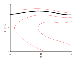
a) b) c)

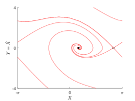
Fig.  4: Phase plane plots illustrating three structurally stable regimes for the damped pendulum. a) The black trajectory corresponds to the stable periodic orbit (when viewed on the cylinder). b) Two fixed points appear in a saddle–node bifurcation. Thus, we have a stable focus coexisting with a stable periodic orbit. c) The periodic orbit disappears in a homoclinic bifurcation. The stable focus remains the only attractor.

Fig.  5: Bifurcation diagram illustrating three qualitatively distinct regimes in the damped pendulum model (3.38), (3.39).

4 The loss of coherence and chimera states

4.1 The overview of synchronization in the second–order KM

In this section, we describe a mechanism for the loss of stability of a two-cluster state due to the loss of synchronization in one of the clusters. We show that this leads to the creation of chimera states. To this end, it is instructive first to review synchronization in a single all–to–all coupled population of second–order phase oscillators:

$$\ddot{u}_{n,i}+\gamma\dot{u}_{n,i}=\xi_{i}+Kn^{-1}\sum_{j=1}^{n}\sin\left(u_{n,j}-u_{n,i}\right),\quad i\in[n],$$ (4.1)

where $\xi_{i}$ are IID RVs taken from a probability distribution with density $g$. Throughout this discussion, we assume that $g$ is a unimodal even function. If the initial conditions are drawn from the continuous probability distribution then the distribution of the phase of oscillators in the extended phase space $\SS\times{\mathbb{R}}\times{\mathbb{R}}$ remains absolutely continuous with respect to the Lebesgue measure for every $t>0$. The density $f(t,u,v,\omega)$ satisfies the following Vlasov equation (cf. [8])

$$\partial_{t}f+\partial_{u}\left(vf\right)+\partial_{v}\left(Vf\right)=0,$$ (4.2)

where

$$V:=\omega-\gamma v+K\int_{{\mathbb{T}}\times{\mathbb{R}}\times{\mathbb{R}}}\sin\left(\phi-u\right)f(t,\phi,\psi,\omega)g(\lambda)d\phi d\psi d\lambda.$$ (4.3)

The Vlasov equation (4.2), (4.3) has a steady state solution:

$$\bar{f}(u,v)={\delta_{\omega/\gamma}(v)\over 2\pi}.$$ (4.4)

It describes the configuration when phases are distributed uniformly over the unit circle, while velocities are localized around $\omega/\gamma$. This is an incoherent or mixing state. Linear stability analysis of (4.2) about $\bar{f}$ shows that there is a critical value $K_{c}>0$ such that the mixing state is stable for $K\in[0,K_{c}]$ and and is unstable for $K>K_{c}$. For $\alpha=0$ the value of $K_{c}$ is known explicitly [6]

$$K_{c}=2\left(\pi g(0)-\int_{\mathbb{R}}{\gamma g(\gamma\omega)\over\gamma^{2}+\omega^{2}}~{}d\omega\right)^{-1}.$$ (4.5)

4.2 The loss of coherence within a cluster

The macro–micro decomposition yields the following picture of cluster dynamics in the second order KM. The macroscopic evolution of two subpopulations is described by the damped pendulum equation (3.38), (3.39). On the other hand the fluctuations in the two subpopulations are described by the system of two coupled Vlasov equations (2.27), (2.28) and (2.29), (2.30). The coupling between (2.27), (2.28) and (2.29), (2.30) is modulated by the group dynamics through $c(t)$ (see (2.25)). For stability of a two-cluster configuration, we need a stable solution of the pendulum equation. In addition, we need fluctuations in both groups to remain small. There are two qualitatively distinct stable states of the equation for the group motion:

A)

a stable fixed point resulting in the phase locked (stationary) clusters (Fig. 4 b,c),

B)

a stable limit cycle resulting in two clusters moving in opposite directions (Fig. 4 a,b).

The corresponding clusters are shown in Fig. 6. For each of this cases, we show that one can desynchronize the oscillators in one cluster without affecting the oscillators in the other cluster.

a)

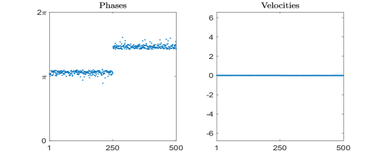
b)

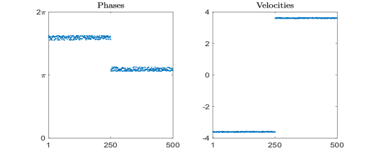
Fig.  6: Two qualitatively distinct types of clusters: a) stationary and b) moving. The corresponding stable states of the pendulum equation (3.38), (3.39) are a stable fixed point and a limit cycle respectively. The values of parameters used for both plots are $\gamma=.1$ and $\omega$ chosen from $\mathcal{N}(\pm.5,.05)$.

We consider stationary clusters first. Recall the damped pendulum equation (3.38), (3.39) governing the group dynamics. For $K>1$, it has a pair of fixed points (Fig. 5), one of which is stable (cf. (3.40)). We suppose that the group dynamics is driven by the stable equilibrium. We will locate parameter regimes where the fluctuations in the two clusters become practically independent. Then we demonstrate that the fluctuations in each cluster can be controlled separately. In particular, we will desynchronize one cluster, while keeping the other one coherent.

We start with the case of $\alpha=0$. When the system (3.38), (3.39) is at the stable equilibrium (cf. (3.40)),

$$U_{2}-U_{1}=\arcsin\left(\frac{1}{K\cos(\alpha)}\right),$$ (4.6)

so $c(t)=\frac{\sqrt{K^{2}-1}}{K}$. Thus, for $K$ just above $1$,

$$0<K-1\ll 1,$$ (4.7)

we have $c(t)\approx 0$. In this regime, the two Vlasov equations describing the coherence in the two clusters are practically decoupled. Thus, we can treat each cluster as a separate population of oscillators and compute the critical values of the coupling strength using (4.5) for each cluster separately. Next we choose the variances of the distributions of intrinsic frequencies $\sigma_{1}^{2}$ and $\sigma_{2}^{2}$ such that

$$K_{c}(\sigma_{1}^{2})<K<K_{c}(\sigma_{2}^{2}).$$

Then for a given value of $K$ the mixing state is stable for the first cluster, while it is unstable for the second cluster. As a result, we get a chimera state with the oscillators in the first cluster distributed uniformly while the oscillators in the second cluster remain synchronized (see Fig. 7).

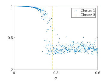
a) b)

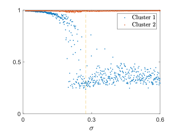
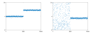
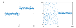
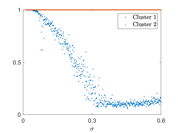
c) d)

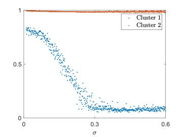
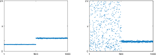
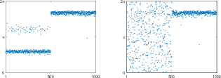
Fig.  7: For $0<K-1\ll 1$ the system for the group dynamics (3.38), (3.39) has a stable fixed point. When the group dynamics is driven by the stable fixed point, $c(t)\approx 0$ (see the text). For a given $K$, we use (4.5) to compute the critical value of the variance $\sigma_{*}^{2},$ at which the incoherent state loses stability. When the variance of the distribution of the intrinsic frequencies for the first cluster is increased beyond $\sigma^{*}$ (dotted line) the first cluster desynchronizes. This results in the formation of chimera state. a) All-to-all coupling and b) ER connectivity with $p=.1$. Other parameters are $K=1.1$ and $\gamma=1$. The same experiment was repeated for $K=2$, $\gamma=.5$, and $\alpha=1.0472$. The results are shown for c) all-to-all coupling and d) ER graph with $p=.5$.

The same idea can be used to generate chimera states for an arbitrary value of $K$ by changing $\alpha$. In this case, $c(t)=\cos(U_{2}-U_{1}+\alpha)$ from (4.6) we have

$$c(t)=\cos\left(\arcsin\left(\frac{1}{K\cos(\alpha)}\right)+\alpha\right).$$

Choosing $\alpha:=\alpha^{\ast}\in(0,\arccos(K^{-1}))$ such that

$$\arcsin\left(\frac{1}{K\cos(\alpha^{\ast})}\right)+\alpha^{\ast}=\frac{\pi}{2}.$$ (4.8)

we can make $c(t)\equiv 0$. With this choice of $\alpha$, the two Vlasov equations decouple as before. We now choose the variances $\sigma_{1,2}^{2}$ sufficiently small so that both clusters are coherent for a given $K>1$. In particular,

$$\max\{K_{c}(\sigma_{1}^{2},\alpha),K_{c}(\sigma_{2}^{2},\alpha)\}<K,$$ (4.9)

i.e., the incoherent state is unstable for each cluster. Note that since the Vlasov equations are uncoupled, we can compute the critical values $K_{c}(\sigma_{1}^{2},\alpha)$ and $K_{c}(\sigma_{1}^{2},\alpha)$ for each cluster separately. Next, we keep $\sigma_{2}^{2}$ fixed and and increase $\sigma_{1}^{2}$ so that

$$K_{c}(\sigma_{2}^{2},\alpha)<K<K_{c}(\sigma_{1}^{2},\alpha).$$ (4.10)

Now the second cluster remains coherent, while the first cluster transitions to the newly stable mixing state, thus, giving rise to a chimera state. The results of this experiment are presented in Figs.  8a and 9.

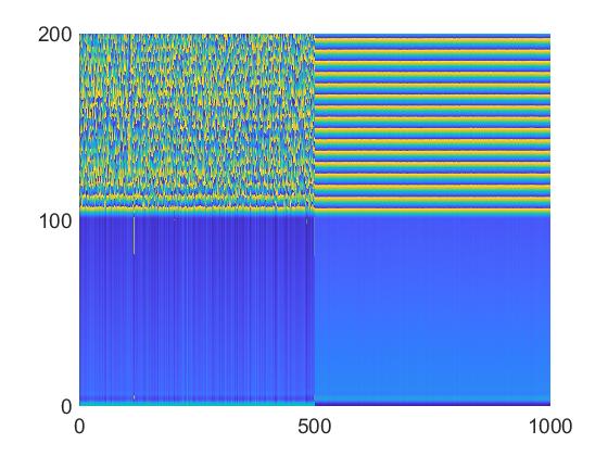
a) b)

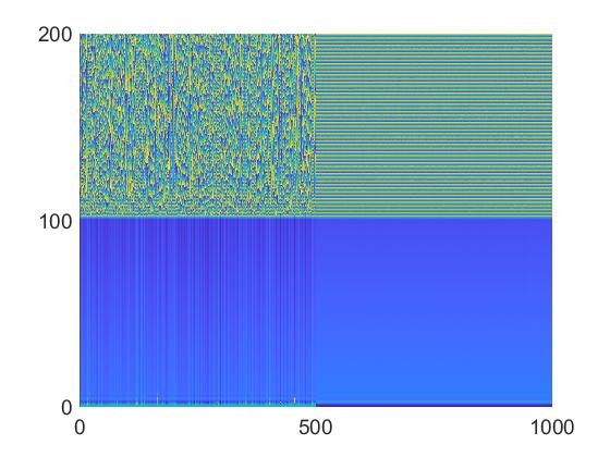
Fig.  8: Plots show the evolution of oscillators (horizontal axis) over time (vertical axis) with phase indicated by color. Before $t=100$, we fix $\alpha=0$. a) At $t=100$ instantaneously let $\alpha=\alpha^{*}$ (the solution of (4.8)). See also Figure 9. b) At $t=100$ let $\alpha$ evolve by (4.11). See also Figure 10. In both cases the first cluster desynchronizes resulting in the emergence of a chimera state. Parameters are $\gamma=1$, $K=5$, and frequencies are chosen from $\mathcal{N}(-.5,.9)$ and $\mathcal{N}(.5,.05)$.

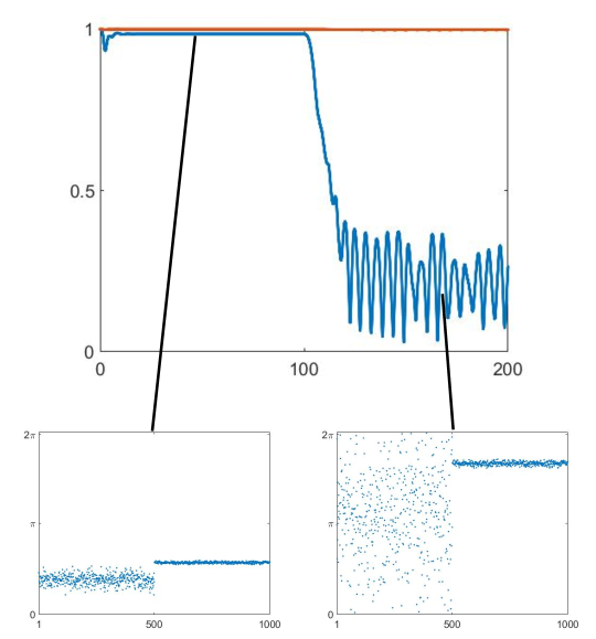
a) b)

Fig.  9: Starting the simulation with $\alpha=0$ fixed, we observe phase-locked solutions. At $t=100$ we instantaneously let $\alpha=\alpha^{*}$ (the solution of (4.8)) and observe the emergence of a chimera state. a) Shows the order parameter of each cluster over time, together with snapshots showing both phase locked and chimera states. b) Shows a snapshot of oscillator velocities from the chimera state. Here $\gamma=1$, $K=5$, and frequencies are chosen from $\mathcal{N}(-.5,.9)$ and $\mathcal{N}(.5,.05)$.

In the numerical experiments above we used the explicit expression of the stable equilibrium (3.40) to compute the value of $\alpha^{\ast}$, for which the coupling coefficient $c(t)$ vanishes (cf. (4.8)). Instead one can use the following adaptive scheme to guide the system into the regime where $c(t)$ becomes very small. To this end, let us add the following differential equation for $\alpha$:

$$\dot{\alpha}=\cos(U_{2}-U_{1}+\alpha).$$ (4.11)

The right–hand side of (4.11) depends on the average values of $u$ computed for the first and the second cluster

$$U_{1}=m^{-1}\sum_{k=1}^{m}u_{k},\;\;U_{2}=l^{-1}\sum_{k=1}^{l}u_{k}.$$ (4.12)

Note that at any fixed point of (4.11), $c(t)=\cos(U_{2}-U_{1}+\alpha)$ is automatically zero. Thus, after short transients we expect that the evolution of $\alpha$ forces $c(t)$ to become very small and to stay small for all future times. We verified this scenario numerically in the experiment illustrated in Figs.  8b and 10.

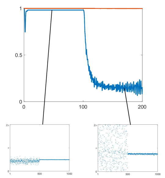
a) b)

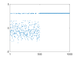
Fig.  10: Starting the simulation with $\alpha=0$ fixed, we observe phase-locked solutions. At $t=100$ we let $\alpha$ evolve by (4.11) and see the emergence of a chimera state. a) Shows the order parameter of each cluster over time, together with snapshots showing both phase locked and chimera states. b) Shows a snapshot of oscillator velocities during chimera state. Here $\gamma=1$, $K=5$, and frequencies are chosen from $\mathcal{N}(-.5,.9)$ and $\mathcal{N}(.5,.05)$.

Finally, we turn to the case when the group dynamics are driven by a limit cycle. In this case, it is easy to find the values of parameters for which the velocity $\dot{U}_{2}-\dot{U}_{1}$ along the limit cycle is sufficiently large and approximately constant (see Fig. 4a). Then $c(t)\approx\cos(\omega t+\tau)$ for some $\omega\gg 1$ and phase shift $\tau$ (Fig. 11a). Note that the average value of $c$ is $0$ and as before, i.e., we effectively have uncoupled equations for the fluctuations in the two clusters. Using this observation, we can construct numerical examples illustrating the loss of stability of two-cluster states leading to chimera states (Fig. 11).

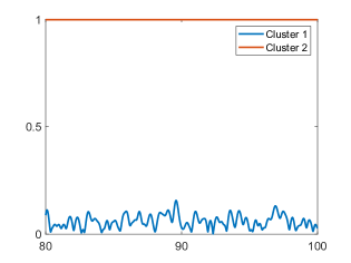
a)
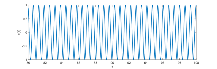
b) c)
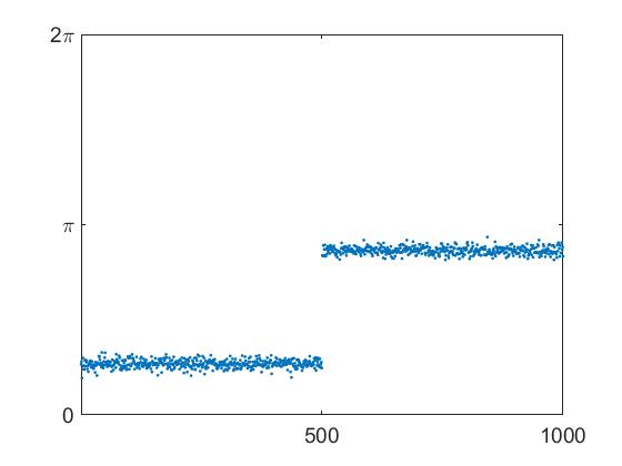
d) e)

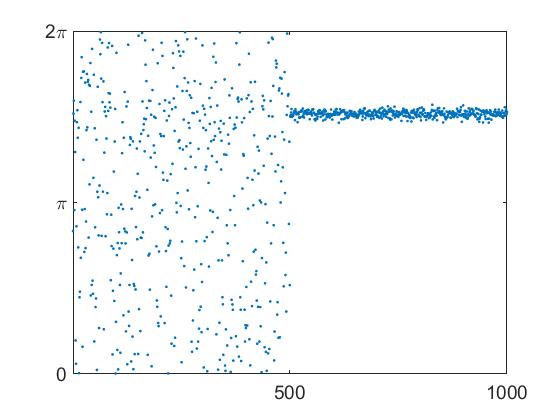
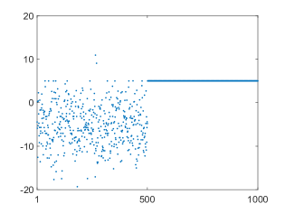
f) g)

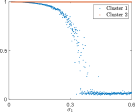
Fig.  11: Taking parameters $\gamma=.1,K=1.5$ we generate two coherent clusters moving in opposite directions rapidly. a) The coupling coefficient $c(t)$ oscillates rapidly around $0$. Taking frequencies chosen from $\mathcal{N}(\pm.5,.05)$ we see both clusters remain synchronized. b) The order parameters for both clusters remain close to $1$ for all times, and c) a snapshot of synchronized clusters. Next taking frequencies of the first cluster from $\mathcal{N}(-.5,.5)$, cluster 1 desynchronizes, while cluster 2 remains synchronous. d) The order parameter for cluster 1 rapidly converges close to zero, but the order parameter for cluster 2 remains close to 1 for all time. e) A snapshot of the resultant chimera and f) a snapshot of oscillator velocities. g) The order parameters of each cluster when frequencies of the first cluster are taken from $\mathcal{N}(-.5,\sigma_{1})$.

5 Discussion

The main contribution of this paper is the general framework for studying stability of clusters in the second order KM with random intrinsic frequencies. We show that the stability of a two-cluster state depends on the stability of the underlying group motion and the stability of coherence within each cluster. The first problem is deterministic. It has already been identified in the analysis of the KM with identical oscillators [5]. The second problem is intrinsically stochastic. To our knowledge, it has not been analyzed in the context of stability of clusters before. We demonstrate that the loss of coherence in one of the clusters leads to the destabilization of the two-cluster state. In contrast to the stability of clusters in the KM with identical oscillators in [5] or the loss of stability of solitary states in [10], the underlying bifurcation is the bifurcation of the steady state of the system of Vlasov PDEs not of the damped pendulum equation, i.e., that this is an infinite-dimensional phenomenon. Interestingly, this leads to the creation of chimera states with one cluster staying coherent and the other incoherent. The emerging chimera states differ from the previously reported ones in several respects. They do not lie close to the border between the regions of the attractive and repulsive coupling like the chimera states in the classical KM (cf. [16]). They do not depend on the block structure of the coupling (adjacency) matrix, as chimera states in [13, 14]. Unlike solitary states in [10], they do not rely on the existence of clusters with equal velocities. The velocities in the incoherent clusters of chimera states shown in Figs. 9, 10, and 11 are distributed over an interval.

The coexistence of coherence and incoherence in the homogeneous networks of coupled oscillators has been the most intriguing feature of chimera states since their discovery in [11]. For large systems, the most comprehensive explanation for such coexistence is based on the Ott-Antonsen Ansatz [16], i.e., it applies to a family of special solutions of the KM. The existence of the weak chimera states as defined in [4] is difficult to verify in large systems with random parameters. At the same time, numerous modeling and experimental studies clearly demonstrate that the coexistence of coherence and incoherence in coupled system is a universal phenomenon. In this paper, we analytically showed the existence of two-cluster states having distinct statistical properties. The distribution of the fluctuations in one cluster can be controlled independently from the distribution in the other cluster. This provides a new mechanism for spatiotemporal patterns with regions with distinct statistical properties and explains formation of chimera states shown in Figs.  8, 9, 10, and 11.

The analysis of this paper can be used to study patterns with $d>2$ clusters. In this case, the problem of stability is reduced to a system of $d-1$ coupled pendulum equations and $d$ coupled Vlasov PDEs. We were able to analyze certain $3-$cluster states (not presented in this paper). However, the complexity of the problem grows rapidly with $d$. We anticipate that symmetry can be used to understand at least certain $d$-clusters for $d>2$. Furthermore, as we remarked earlier, our approach naturally extends to systems on more general random graphs (cf. [12]). The studies of the classical KM of coupled phase oscillators made substantial contribution to our understanding of synchronization in coupled systems [17]. The second order KM holds an equal potential for the formation of clusters in large coupled dynamical systems.

Acknowledgements. This work was supported in part by NSF grant DMS 1715161 (to GM). Numerical simulations were completed using the high performance computing cluster (ELSA) at the School of Science, The College of New Jersey. Funding of ELSA is provided in part by National Science Foundation OAC-1828163. MSM was additionally supported by a Support of Scholarly Activities Grant at The College of New Jersey.

References

- [1] D.M. Abrams and S.H. Strogatz, Chimera states in a ring of nonlocally coupled oscillators, Internat. J. Bifur. Chaos Appl. Sci. Engrg. 16 (2006), no. 1, 21–37.
- [2] A. A. Andronov, A. A. Vitt, and S. È. Khaĭkin, Theory of oscillators, Dover Publications, Inc., New York, 1987, Translated from the Russian by F. Immirzi, Reprint of the 1966 translation.
- [3] M. Antoni and S. Ruffo, Clustering and relaxation in hamiltonian long-range dynamics, Phys. Rev. E 52 (1995), 2361–2374.
- [4] P. Ashwin and O. Burylko, Weak chimeras in minimal networks of coupled phase oscillators, Chaos 25 (2015), no. 1, 013106, 9.
- [5] I. V. Belykh, B. N. Brister, and V. N. Belykh, Bistability of patterns of synchrony in kuramoto oscillators with inertia, Chaos: An Interdisciplinary Journal of Nonlinear Science 26 (2016), no. 9, 094822.
- [6] H. Chiba, unpublished notes.
- [7] H. Chiba, A proof of the Kuramoto conjecture for a bifurcation structure of the infinite-dimensional Kuramoto model, Ergodic Theory Dynam. Systems 35 (2015), no. 3, 762–834.
- [8] H. Chiba and G. S. Medvedev, The mean field analysis of the Kuramoto model on graphs I. The mean field equation and transition point formulas, Discrete Contin. Dyn. Syst. 39 (2019), no. 1, 131–155.
- [9] F. Dörfler and F. Bullo, Synchronization and transient stability in power networks and nonuniform Kuramoto oscillators, SIAM J. Control Optim. 50 (2012), no. 3, 1616–1642. MR 2968069
- [10] P. Jaros, S. Brezetsky, R. Levchenko, D. Dudkowski, T. Kapitaniak, and Yu. Maistrenko, Solitary states for coupled oscillators with inertia, Chaos 28 (2018), no. 1, 011103, 7.
- [11] Y. Kuramoto and D. Battogtokh, Coexistence of coherence and incoherence in nonlocally coupled phase oscillators, Nonlinear Phenomena in Complex Systems 5 (2002), 380–385.
- [12] G. S. Medvedev, The continuum limit of the Kuramoto model on sparse random graphs, Commun. Math. Sci. 17 (2019), no. 4, 883–898. MR 4030504
- [13] S. Olmi, Chimera states in coupled Kuramoto oscillators with inertia, Chaos 25 (2015), no. 12, 123125, 13.
- [14] S. Olmi, E. A. Martens, S. Thutupalli, and A. Torcini, Intermittent chaotic chimeras for coupled rotators, Phys. Rev. E 92 (2015), 030901.
- [15] O. E. Omel’chenko, The mathematics behind chimera states, Nonlinearity 31 (2018), no. 5, R121–R164.
- [16] O.E. Omelchenko, Coherence-incoherence patterns in a ring of non-locally coupled phase oscillators, Nonlinearity 26 (2013), no. 9, 2469.
- [17] F. A. Rodrigues, T. K. DM. Peron, P. Ji, and J. Kurths, The Kuramoto model in complex networks, Physics Reports 610 (2016), 1 – 98, The Kuramoto model in complex networks.
- [18] F. Salam, J. Marsden, and P. Varaiya, Arnold diffusion in the swing equations of a power system, IEEE Transactions on Circuits and Systems 31 (1984), no. 8, 673–688.
- [19] S. H. Strogatz and R. E. Mirollo, Stability of incoherence in a population of coupled oscillators, J. Statist. Phys. 63 (1991), no. 3-4, 613–635.
- [20] H.-A. Tanaka, M. de Sousa Vieira, A. J. Lichtenberg, M. A. Lieberman, and S. Oishi, Stability of synchronized states in one-dimensional networks of second order PLLs, Internat. J. Bifur. Chaos Appl. Sci. Engrg. 7 (1997), no. 3, 681–690.
- [21] L. Tumash, S. Olmi, and E. Schöll, Stability and control of power grids with diluted network topology, Chaos: An Interdisciplinary Journal of Nonlinear Science 29 (2019), no. 12, 123105.