Minimal Model for Fast Scrambling
Abstract
We study quantum information scrambling in spin models with both long-range all-to-all and short-range interactions. We argue that a simple global, spatially homogeneous interaction together with local chaotic dynamics is sufficient to give rise to fast scrambling, which describes the spread of quantum information over the entire system in a time that is logarithmic in the system size. This is illustrated in two tractable models: (1) a random circuit with Haar random local unitaries and a global interaction and (2) a classical model of globally coupled non-linear oscillators. We use exact numerics to provide further evidence by studying the time evolution of an out-of-time-order correlator and entanglement entropy in spin chains of intermediate sizes. Our results pave the way towards experimental investigations of fast scrambling and aspects of quantum gravity with quantum simulators.
Introduction.—The study of quantum information scrambling has recently attracted significant attention due to its relation to quantum chaos and thermalization of isolated many-body systems Deutsch (1991); Srednicki (1994); Rigol et al. (2008) as well as the dynamics of black holes Hayden and Preskill (2007); Lashkari et al. (2013); Shenker and Stanford (2014); Maldacena et al. (2016). Scrambling refers to the spread of an initially local quantum information over the many-body degrees of freedom of the entire system, rendering it inaccessible to local measurements. Scrambling is also related to the Heisenberg dynamics of local operators, and can be probed via the squared commutator of two local and Hermitian operators , at positions and respectively,
| (1) |
where is the Heisenberg evolved operator. The growth of the squared commutator corresponds to increasing in size and complexity, leading it to fail to commute with . In a local quantum chaotic system, typically spreads ballistically, exhibiting rapid growth ahead of the wavefront and saturation behind, at late times Patel et al. (2017); Xu and Swingle (2019, 2020).
Of particular interest are the so-called fast scramblers, systems where reaches for all in a time , with being the number of degrees of freedom. Among the best known examples are black holes, which are conjectured to be the fastest scramblers in nature Sekino and Susskind (2008); Lashkari et al. (2013); Shenker and Stanford (2014); Maldacena et al. (2016), as well as the Sachdev-Ye-Kitaev (SYK) Sachdev and Ye (1993); Kitaev (2015) model and other related holographic models Danshita et al. (2017); Chen et al. (2018); Chew et al. (2017); Gu et al. (2017).
Recent advances in the development of coherent quantum simulators have enabled the study of out-of-equilibrium dynamics of spin models with controllable interactions Cirac and Zoller (2012), making them ideal platforms to experimentally study information scrambling. Several experiments have already been performed Li et al. (2017); Gärttner et al. (2017); Wei et al. (2018); Landsman et al. (2019); Joshi et al. (2020); Blok et al. (2020), probing scrambling in either local or non-chaotic systems. The experimental observation of fast scrambling remains challenging however, particularly because few systems are known to be fast scramblers, and those that are, like the SYK model, are highly non-trivial, involving random couplings and many-body interactions. Some recent proposals suggested that spin models with non-local interactions can exhibit fast scrambling Swingle et al. (2016); Marino and Rey (2019); Bentsen et al. (2019), albeit with complicated and inhomogeneous interactions.
In this paper, we argue that the simplest possible global interaction, together with chaotic dynamics, are sufficient to make a spin model fast scrambling. We consider spin-1/2 chains with Hamiltonians of the form
| (2) |
where is the Pauli operator acting on site and is a Hamiltonian with only local interactions that ensures that the full is chaotic. We note that such global interactions are ubiquitous in ultracold atoms in optical cavities Sørensen and Mølmer (2002); Chaudhury et al. (2007); Fernholz et al. (2008); Leroux et al. (2010); Schleier-Smith et al. (2010), and also in ion traps Sawyer et al. (2012); Britton et al. (2012); Wang et al. (2013); Bohnet et al. (2016).
We first show that this effect is generic, by studying two models, a random quantum circuit and a classical model, both designed to mimic the universal dynamics of Eq. 2. We then provide numerical evidence for fast scrambling for a particular time-independent quantum Hamiltonian. Finally, we discuss possible experimental realizations.
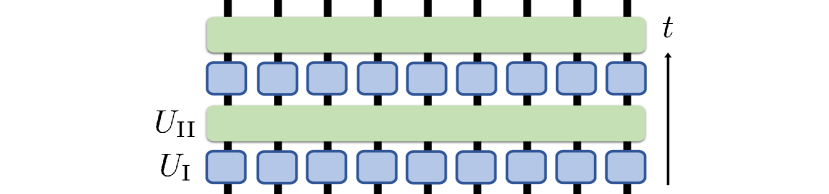
Random circuit model.—As a proof-of-principle, we consider a system of spin-1/2 sites, with dynamics generated by a random quantum circuit (see Fig. 1) inspired by the Hamiltonian in Eq. 2. While less physical than the Hamiltonian model, it has the advantage of being exactly solvable while providing intuition about generic many-body chaotic systems with similar features.
The time-evolution operator is where a single-time-step update consists of the two layers
| (3) |
where each is an independent Haar-random single-site unitary. The two layers in Eq. 3 are motivated by the two terms in Eq. 2, with the Haar-random unitaries replacing .
We are interested in the operator growth of an initially simple operator . At any point in time, the Heisenberg operator can be decomposed as , where is a string composed of the Pauli matrices and the identity, forming a basis for . As in random brickwork models Nahum et al. (2018); von Keyserlingk et al. (2018) and random Brownian models Xu and Swingle (2019), the Haar-averaged probabilities , encoding the time evolution of , themselves obey a linear equation
| (4) |
Here, is a stochastic matrix describing a fictitious Markov process Dahlsten et al. (2007); Žnidarič (2008). The average probabilities fully determine the growth of the average of in Eq. 1 (see Supplemental Material (SM) sup ). Because of the Haar unitaries and the simple uniform interaction in Eq. 3, is highly degenerate and only depends on the total weights of the strings , counting the number of non-identity operators, i.e , and on the number of sites where both and are non-identity, i.e , and is given by (see SM for derivation sup ) 111The term with is assumed to be . See sup .
| (5) | ||||
If we further assume that starts out as a single site operator on site , then throughout the evolution, only depend on the total operator weight , and the weight on site , which we denote by . We thus introduce the operator weight probability at time ,
| (6) |
which gives the probability of having total weight and weight on site 1.
The time evolution of is given by the master equation
| (7) |
where the matrix is
| (8) | ||||
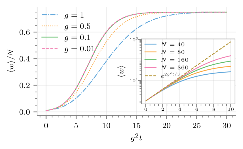
The transition matrix , scaling only linearly with , allows us to efficiently simulate the dynamics for large system sizes (see Fig. 2).
To proceed analytically, we Taylor-expand Eq. 5 to leading order in , which gives rise to a closed master equation for the total operator weight probability ,
| (9) | ||||
which is similar to random Brownian models Xu and Swingle (2019); Zhou and Chen (2019) and shows that, at , can change by at most in a single step. Assuming that varies slowly with respect to and , we can approximate the above equation by a Fokker-Planck equation (rescaling time )
| (10) |
where the drift and diffusion coefficients are (dropping higher order terms )
| (11) |
This equation describes the rapid growth of an initially localized distribution, followed by a broadening and finally saturation (see Fig. 2 and SM sup for more details). At early time, the term in the drift coefficient dominates, giving rise to exponential growth of the mean operator weight , which agrees with the full numerical solution of the master equation, as can be seen in Fig. 2. The mean weight is related to the infinite-temperature squared-commutator in Eq. 1 (averaged over different circuits) via sup . Since grows exponentially with time, reaches and reaches when , thus establishing that this model is fast scrambling. Note that the normalization in Eqs. 2 and 3 is crucial. Had we chosen instead , the Lyapunov exponent would have been and the scrambling time would have been .
Classical Model.—Let us now consider a different setting that also allows to probe the basic timescales involved, and shows that randomness is not required. A convenient tractable choice is a classical model consisting of globally coupled non-linear oscillators. Note that the analogs of out-of-time-order correlators (OTOCs) have been studied in a variety of classical models Rozenbaum et al. (2017); Bilitewski et al. (2018); Chávez-Carlos et al. (2019); Jalabert et al. (2018); Yan et al. (2020); Marino and Rey (2019) and have been shown to capture the scrambling dynamics of quantum models like the SYK model Kurchan (2018); Schmitt et al. (2019); Scaffidi and Altman (2019).
Consider a -dimensional phase space with coordinates (positions) and (momenta) for with canonical structure specified by the Poisson brackets . The Hamiltonian is where
| (12) | ||||
| (13) |
The timescales for the growth of perturbations under dynamics may be understood in two stages. First, can be solved exactly; this combination of terms provides the non-locality. The remaining term renders the dynamics chaotic, provided is large enough. The dynamics of causes a localized perturbation to spread to every oscillator with non-local amplitude in a time of order . Then conventional local chaos can amplify this -sized perturbation to order-one size in a time of order , where is some typical Lyapunov exponent.
At the quadratic level, the uniform mode, , is decoupled from the remaining modes of the chain. Hence, the propagation of any perturbation is a superposition of the motion due to the local terms and the special dynamics of the uniform mode. Since the local terms cannot induce non-local perturbations, we may focus on the dynamics of the uniform mode. The uniform mode’s equation of motion is with solution
| (14) |
A localized perturbation on site with zero initial time derivative can be written as , where represents the uniform mode, , and is orthogonal to the uniform mode. The orthogonal mode evolves in a local fashion, hence . For oscillators far from the initial local perturbation, the dynamics is given by
| (15) |
Thus, after a time , any localized perturbation has spread to distant sites with amplitude .
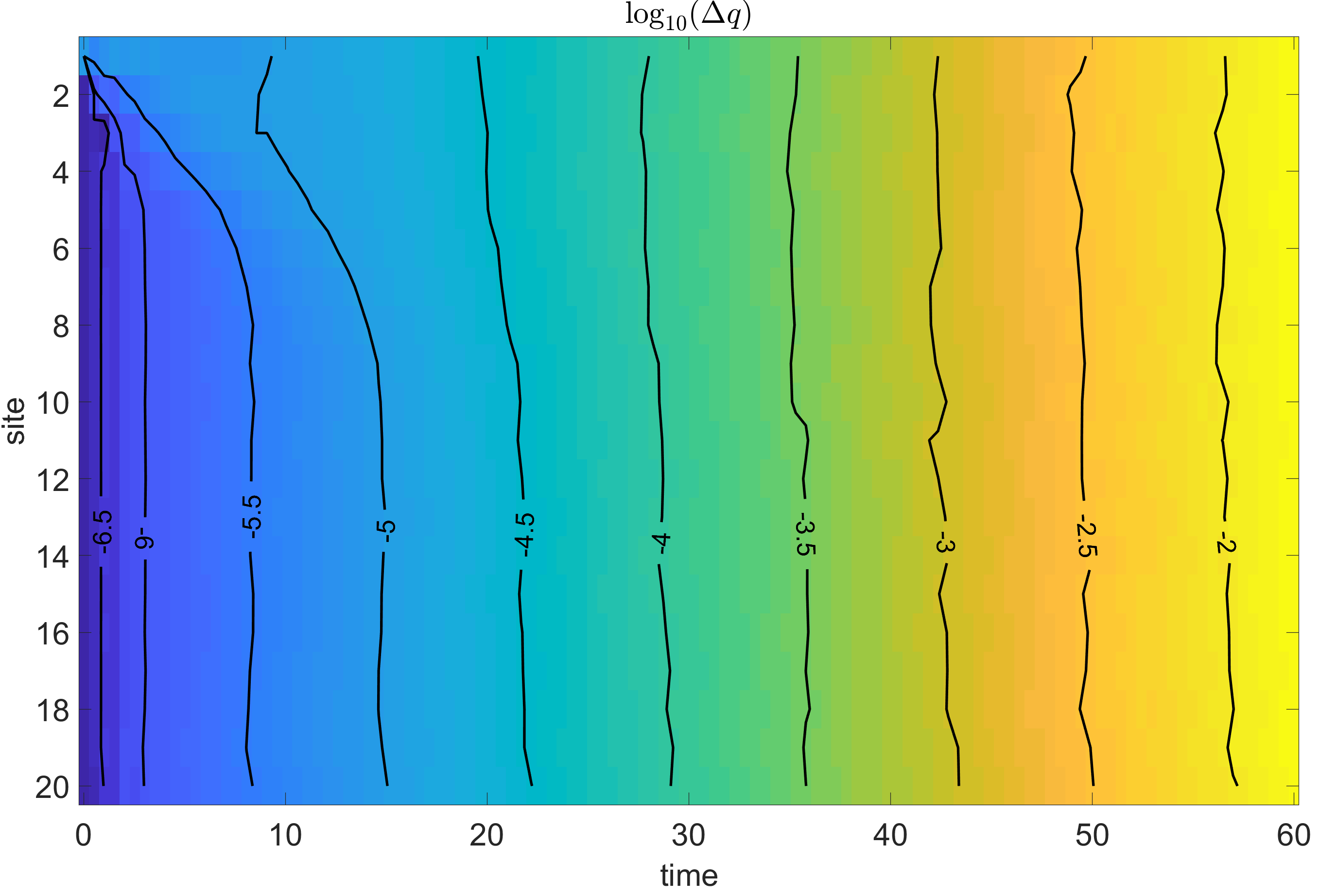
The inclusion of renders the equations of motion non-linear and the system chaotic in at least part of the phase space. We leave a detailed study of the classical chaotic dynamics of this model to the future, but as can be seen in Fig. 3, a numerical solution of the equations of motion displays sensitivity to initial conditions.
The precise protocol is as follows. We compare the dynamics of two configurations, and , averaged over many initial conditions. The initial condition of configuration one has each oscillator start at rest from a random amplitude drawn uniformly and independently from . Configuration two is identical to configuration one except that for . Both configurations are evolved in time and the difference is computed and averaged over different initial conditions. Figure 3 shows this average of for with , , and . Because the system can generate an -sized perturbation on all sites in a short time, the subsequent uniform exponential growth implies that any local perturbation will become order one on all sites after a time .
The above analysis corresponds to the classical limit of coupled quantum oscillators where some effective dimensionless Planck’s constant vanishes, . In the opposite limit of large at fixed , the dynamics of quantum OTOCs can be obtained from the corresponding classical Lyapunov growth up to a timescale of order . At later times, one needs to consider fully quantum local dynamics. If one imagines breaking the system up into local clusters and if each cluster can be viewed as a quantum chaotic system with random-matrix-like energy levels, a dynamical system not unlike the random circuit model above is obtained.
Chaos and level statistics.—Having established fast scrambling in both the random circuit and the classical model, we now return to the quantum spin model of Eq. 2. We first examine whether such a model is chaotic, which is a necessary condition for it being fast scrambling. For the local Hamiltonian part, we consider the mixed-field Ising chain
| (16) |
A standard approach to identify a transition from integrability to quantum chaos is based on a comparison of energy-level-spacing statistics with Poisson and Wigner-Dyson distributions. Another convenient metric is the average ratio of consecutive level spacings Atas et al. (2013) , where , , , and are the eigenvalues ordered such that .
As was already suggested in Ref. Lerose et al. (2018) for a similar model, we find that the longitudinal field is unnecessary, and the full system can have Wigner-Dyson statistics even for , in which case is integrable. The resulting Hamiltonian reads
| (17) |
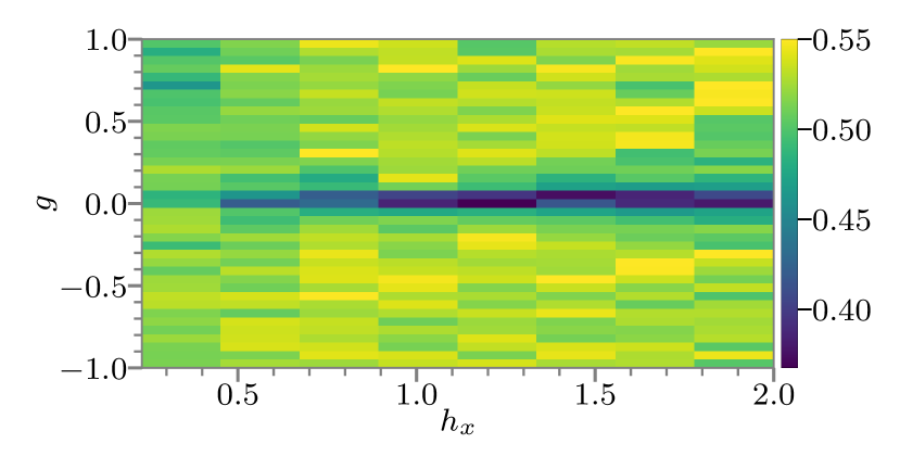
Average adjacent-level-spacing ratio changes from for Poisson level statistics to for Wigner-Dyson level statistics in the Gaussian Orthogonal Ensemble (GOE) Atas et al. (2013). In the vicinity of , (see Fig. 4) shows proximity to Poisson statistics, while, for , the level statistics agree with those of the GOE.
Out-of-time-order correlator and entanglement growth.—We now study the dynamics of an OTOC and entanglement entropy in the spin chain. We consider the following OTOC
| (18) |
which is related to Eq. 1 by . The expectation value is evaluated in a Haar-random pure state, which approximates the infinite-temperature OTOC, but enables us to reach larger system sizes Luitz and Bar Lev (2017).
In Fig. 5(a), we show the OTOC for an open chain of spins for both the local model, governed by only, and the non-local model in Eq. 17, which includes the global interaction. In the local case, the OTOC spreads ballistically, forming a linear light cone. In contrast, in the non-local case, the spreading is super-ballistic and is approximately independent of , as expected for a fast scrambler. As we discussed in the context of the classical model, a necessary condition for fast scrambling is that, before the onset of exponential growth, the decay of correlations with should be at most algebraic () and not exponential. In Fig. 5(b), we verify that this is the case for the non-local model, showing that between the two ends of the chain after a fixed time.
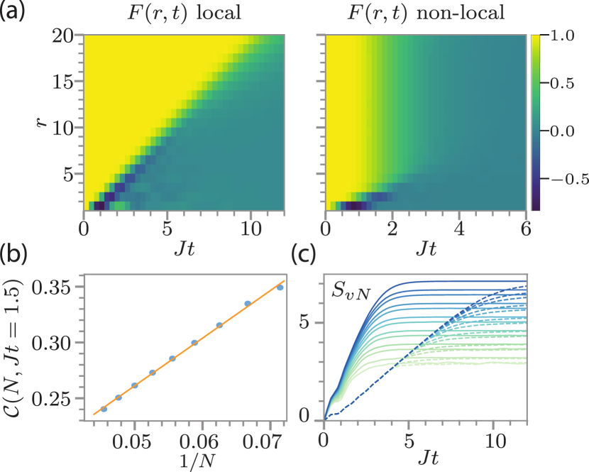
Figure 5(c) shows the half-cut entanglement entropy following a quench starting from the state for both models. For the local model, the entanglement grows linearly in time before saturating, whereas the non-local model shows a significant speed up. Moreover, in the non-local model, the growth rate clearly increases with the system size, further supporting our claim.
Experimental realization.—The Hamiltonian in Eq. 17, and many variations of it, can be experimentally realized in a variety of platforms. A natural realization is with Rydberg dressing of neutral atoms Honer et al. (2010); Graß et al. (2018); Pupillo et al. (2010); Glaetzle et al. (2012). The spin can be encoded in two ground states with one of them dressed to two Rydberg states such that one of the Rydberg states leads to all-to-all interactions and the second to nearest-neighbor interactions. Other similar spin models can be realized with cavity-QED setups, using photon-mediated all-to-all interactions Sørensen and Mølmer (2002); Leroux et al. (2010); Gopalakrishnan et al. (2011); Strack and Sachdev (2011) of the or -Heisenberg form Swingle et al. (2016); Bentsen et al. (2019) together with nearest-neighbor interactions achieved by Rydberg-dressing one of the grounds states Gelhausen et al. (2016); Zhu et al. (2019). Other possibilities include a chain of coupled superconducting qubits, with all-to-all flip-flop interactions mediated via a common bus Majer et al. (2007); Zhu et al. (2016); Onodera et al. (2019) or trapped ions Sawyer et al. (2012); Britton et al. (2012); Wang et al. (2013); Genway et al. (2014); Bohnet et al. (2016).
Conclusion and outlook.—In this paper, we argued that a single global interaction together with local chaotic dynamics is sufficient to give rise to fast scrambling. While fast scrambling is intrinsically difficult to study numerically, our numerical evidence, together with the semi-classical analysis and the exactly solvable random circuit, provide a compelling argument in favor of our claim. Our models do not require disordered or inhomogeneous couplings and are within reach of current state-of-the-art quantum simulators. Thus, an experimental implementation of the spin model could test our claims on much larger systems sizes, something that may very well be impossible to do on a classical computer. This can pave the way towards experimental investigations of aspects of quantum gravity.
Future theoretical work may include a more systematic analysis of the -dependence of various timescales, e.g. for entanglement growth, and of the behaviour of the OTOC at low temperatures. It is also interesting to investigate whether similar conclusions can be reached without perfectly uniform global interactions, for example with power-law decaying interactions.
Acknowledgements.
We thank A. Lucas for useful discussions, especially regarding the normalization of the global interactions. We acknowledge discussions with S. Xu at early stages of this work and P. Titum for pointing out the Hamiltonian [Eq. 17] to us. R.B., P.B., Y.A.K., and A.V.G. acknowledge funding by the NSF PFCQC program, DoE ASCR Quantum Testbed Pathfinder program (award No. DE-SC0019040), DoE BES Materials and Chemical Sciences Research for Quantum Information Science program (award No. DE-SC0019449), DoE ASCR Accelerated Research in Quantum Computing program (award No. DE-SC0020312), AFOSR MURI, AFOSR, ARO MURI, NSF PFC at JQI, and ARL CDQI. R.B. acknowledges support of NSERC and FRQNT of Canada. B.G.S. is supported in part by the U.S. Department of Energy, Office of Science, Office of High Energy Physics QuantISED Award de-sc0019380.Note added. We would like to draw the reader’s attention to two related parallel works which appeared recently: by Li, Choudhury, and Liu Li et al. (2020), on fast scrambling with similar spin models; and by Yin and Lucas Yin and Lucas (2020), on lower bounds of the scrambling time in similar spin models.
References
- Deutsch (1991) J. M. Deutsch, Quantum statistical mechanics in a closed system, Phys. Rev. A 43, 2046 (1991).
- Srednicki (1994) M. Srednicki, Chaos and quantum thermalization, Phys. Rev. E 50, 888 (1994).
- Rigol et al. (2008) M. Rigol, V. Dunjko, and M. Olshanii, Thermalization and its mechanism for generic isolated quantum systems, Nature 452, 854 (2008).
- Hayden and Preskill (2007) P. Hayden and J. Preskill, Black holes as mirrors: quantum information in random subsystems, J. High Energy Phys. 2007 (09), 120.
- Lashkari et al. (2013) N. Lashkari, D. Stanford, M. Hastings, T. Osborne, and P. Hayden, Towards the fast scrambling conjecture, J. High Energy Phys. 2013 (4), 22.
- Shenker and Stanford (2014) S. H. Shenker and D. Stanford, Black holes and the butterfly effect, J. High Energy Phys. 2014 (3), 67.
- Maldacena et al. (2016) J. Maldacena, S. H. Shenker, and D. Stanford, A bound on chaos, J. High Energy Phys. 2016 (8), 106.
- Patel et al. (2017) A. A. Patel, D. Chowdhury, S. Sachdev, and B. Swingle, Quantum Butterfly Effect in Weakly Interacting Diffusive Metals, Phys. Rev. X 7, 031047 (2017).
- Xu and Swingle (2019) S. Xu and B. Swingle, Locality, Quantum Fluctuations, and Scrambling, Phys. Rev. X 9, 031048 (2019).
- Xu and Swingle (2020) S. Xu and B. Swingle, Accessing scrambling using matrix product operators, Nat. Phys. 16, 199 (2020).
- Sekino and Susskind (2008) Y. Sekino and L. Susskind, Fast scramblers, J. High Energy Phys. 2008 (10), 065.
- Sachdev and Ye (1993) S. Sachdev and J. Ye, Gapless spin-fluid ground state in a random quantum Heisenberg magnet, Phys. Rev. Lett. 70, 3339 (1993).
- Kitaev (2015) A. Kitaev, A simple model of quantum holography (2015), in KITP Program: Entanglement in Strongly-Correlated Quantum Matter.
- Danshita et al. (2017) I. Danshita, M. Hanada, and M. Tezuka, Creating and probing the Sachdev–Ye–Kitaev model with ultracold gases: Towards experimental studies of quantum gravity, Prog. Theor. Exp. Phys. 2017, 83 (2017).
- Chen et al. (2018) A. Chen, R. Ilan, F. de Juan, D. I. Pikulin, and M. Franz, Quantum Holography in a Graphene Flake with an Irregular Boundary, Phys. Rev. Lett. 121, 036403 (2018).
- Chew et al. (2017) A. Chew, A. Essin, and J. Alicea, Approximating the Sachdev-Ye-Kitaev model with Majorana wires, Phys. Rev. B 96, 121119 (2017).
- Gu et al. (2017) Y. Gu, X.-L. Qi, and D. Stanford, Local criticality, diffusion and chaos in generalized Sachdev-Ye-Kitaev models, J. High Energy Phys. 2017 (5), 125.
- Cirac and Zoller (2012) J. I. Cirac and P. Zoller, Goals and opportunities in quantum simulation, Nat. Phys. 8, 264 (2012).
- Li et al. (2017) J. Li, R. Fan, H. Wang, B. Ye, B. Zeng, H. Zhai, X. Peng, and J. Du, Measuring Out-of-Time-Order Correlators on a Nuclear Magnetic Resonance Quantum Simulator, Phys. Rev. X 7, 031011 (2017).
- Gärttner et al. (2017) M. Gärttner, J. G. Bohnet, A. Safavi-Naini, M. L. Wall, J. J. Bollinger, and A. M. Rey, Measuring out-of-time-order correlations and multiple quantum spectra in a trapped-ion quantum magnet, Nat. Phys. 13, 781 (2017).
- Wei et al. (2018) K. X. Wei, C. Ramanathan, and P. Cappellaro, Exploring Localization in Nuclear Spin Chains, Phys. Rev. Lett. 120, 070501 (2018).
- Landsman et al. (2019) K. A. Landsman, C. Figgatt, T. Schuster, N. M. Linke, B. Yoshida, N. Y. Yao, and C. Monroe, Verified quantum information scrambling, Nature 567, 61 (2019).
- Joshi et al. (2020) M. K. Joshi, A. Elben, B. Vermersch, T. Brydges, C. Maier, P. Zoller, R. Blatt, and C. F. Roos, Quantum information scrambling in a trapped-ion quantum simulator with tunable range interactions, arXiv:2001.02176 (2020).
- Blok et al. (2020) M. S. Blok, V. V. Ramasesh, T. Schuster, K. O’Brien, J. M. Kreikebaum, D. Dahlen, A. Morvan, B. Yoshida, N. Y. Yao, and I. Siddiqi, Quantum Information Scrambling in a Superconducting Qutrit Processor, arXiv:2003.03307 (2020).
- Swingle et al. (2016) B. Swingle, G. Bentsen, M. Schleier-Smith, and P. Hayden, Measuring the scrambling of quantum information, Phys. Rev. A 94, 040302 (2016).
- Marino and Rey (2019) J. Marino and A. M. Rey, Cavity-QED simulator of slow and fast scrambling, Phys. Rev. A 99, 051803 (2019).
- Bentsen et al. (2019) G. Bentsen, T. Hashizume, A. S. Buyskikh, E. J. Davis, A. J. Daley, S. S. Gubser, and M. Schleier-Smith, Treelike Interactions and Fast Scrambling with Cold Atoms, Phys. Rev. Lett. 123, 130601 (2019).
- Sørensen and Mølmer (2002) A. S. Sørensen and K. Mølmer, Entangling atoms in bad cavities, Phys. Rev. A 66, 022314 (2002).
- Chaudhury et al. (2007) S. Chaudhury, S. Merkel, T. Herr, A. Silberfarb, I. H. Deutsch, and P. S. Jessen, Quantum Control of the Hyperfine Spin of a Cs Atom Ensemble, Phys. Rev. Lett. 99, 163002 (2007).
- Fernholz et al. (2008) T. Fernholz, H. Krauter, K. Jensen, J. F. Sherson, A. S. Sørensen, and E. S. Polzik, Spin squeezing of atomic ensembles via nuclear-electronic spin entanglement, Phys. Rev. Lett. 101, 073601 (2008).
- Leroux et al. (2010) I. D. Leroux, M. H. Schleier-Smith, and V. Vuletić, Implementation of Cavity Squeezing of a Collective Atomic Spin, Phys. Rev. Lett. 104, 073602 (2010).
- Schleier-Smith et al. (2010) M. H. Schleier-Smith, I. D. Leroux, and V. Vuletić, Squeezing the collective spin of a dilute atomic ensemble by cavity feedback, Phys. Rev. A 81, 021804 (2010).
- Sawyer et al. (2012) B. C. Sawyer, J. W. Britton, A. C. Keith, C.-C. J. Wang, J. K. Freericks, H. Uys, M. J. Biercuk, and J. J. Bollinger, Spectroscopy and Thermometry of Drumhead Modes in a Mesoscopic Trapped-Ion Crystal Using Entanglement, Phys. Rev. Lett. 108, 213003 (2012).
- Britton et al. (2012) J. W. Britton, B. C. Sawyer, A. C. Keith, C.-C. J. Wang, J. K. Freericks, H. Uys, M. J. Biercuk, and J. J. Bollinger, Engineered two-dimensional Ising interactions in a trapped-ion quantum simulator with hundreds of spins, Nature 484, 489 (2012).
- Wang et al. (2013) C.-C. J. Wang, A. C. Keith, and J. K. Freericks, Phonon-mediated quantum spin simulator employing a planar ionic crystal in a Penning trap, Phys. Rev. A 87, 013422 (2013).
- Bohnet et al. (2016) J. G. Bohnet, B. C. Sawyer, J. W. Britton, M. L. Wall, A. M. Rey, M. Foss-Feig, and J. J. Bollinger, Quantum spin dynamics and entanglement generation with hundreds of trapped ions, Science 352, 1297 (2016).
- Nahum et al. (2018) A. Nahum, S. Vijay, and J. Haah, Operator Spreading in Random Unitary Circuits, Phys. Rev. X 8, 021014 (2018).
- von Keyserlingk et al. (2018) C. W. von Keyserlingk, T. Rakovszky, F. Pollmann, and S. L. Sondhi, Operator Hydrodynamics, OTOCs, and Entanglement Growth in Systems without Conservation Laws, Phys. Rev. X 8, 021013 (2018).
- Dahlsten et al. (2007) O. C. O. Dahlsten, R. Oliveira, and M. B. Plenio, The emergence of typical entanglement in two-party random processes, J. Phys. A Math. Theor. 40, 8081 (2007).
- Žnidarič (2008) M. Žnidarič, Exact convergence times for generation of random bipartite entanglement, Phys. Rev. A 78, 032324 (2008).
- (41) See Supplemental Material for additional details concerning the random circuit including the derivation, which includes Zhang (2014).
- Zhang (2014) L. Zhang, Matrix integrals over unitary groups: An application of schur-weyl duality (2014), arXiv:1408.3782 [quant-ph] .
- Note (1) The term with is assumed to be . See sup .
- Zhou and Chen (2019) T. Zhou and X. Chen, Operator dynamics in a Brownian quantum circuit, Phys. Rev. E 99, 052212 (2019).
- Rozenbaum et al. (2017) E. B. Rozenbaum, S. Ganeshan, and V. Galitski, Lyapunov exponent and out-of-time-ordered correlator’s growth rate in a chaotic system, Phys. Rev. Lett. 118, 086801 (2017).
- Bilitewski et al. (2018) T. Bilitewski, S. Bhattacharjee, and R. Moessner, Temperature dependence of the butterfly effect in a classical many-body system, Phys. Rev. Lett. 121, 250602 (2018).
- Chávez-Carlos et al. (2019) J. Chávez-Carlos, B. López-del Carpio, M. A. Bastarrachea-Magnani, P. Stránský, S. Lerma-Hernández, L. F. Santos, and J. G. Hirsch, Quantum and classical lyapunov exponents in atom-field interaction systems, Phys. Rev. Lett. 122, 024101 (2019).
- Jalabert et al. (2018) R. A. Jalabert, I. García-Mata, and D. A. Wisniacki, Semiclassical theory of out-of-time-order correlators for low-dimensional classically chaotic systems, Phys. Rev. E 98, 062218 (2018).
- Yan et al. (2020) B. Yan, L. Cincio, and W. H. Zurek, Information Scrambling and Loschmidt Echo, Phys. Rev. Lett. 124, 160603 (2020).
- Kurchan (2018) J. Kurchan, Quantum Bound to Chaos and the Semiclassical Limit, J. Stat. Phys. 171, 965 (2018).
- Schmitt et al. (2019) M. Schmitt, D. Sels, S. Kehrein, and A. Polkovnikov, Semiclassical echo dynamics in the sachdev-ye-kitaev model, Phys. Rev. B 99, 134301 (2019).
- Scaffidi and Altman (2019) T. Scaffidi and E. Altman, Chaos in a classical limit of the sachdev-ye-kitaev model, Phys. Rev. B 100, 155128 (2019).
- Atas et al. (2013) Y. Y. Atas, E. Bogomolny, O. Giraud, and G. Roux, Distribution of the Ratio of Consecutive Level Spacings in Random Matrix Ensembles, Phys. Rev. Lett. 110, 084101 (2013).
- Lerose et al. (2018) A. Lerose, J. Marino, B. Žunkovič, A. Gambassi, and A. Silva, Chaotic Dynamical Ferromagnetic Phase Induced by Nonequilibrium Quantum Fluctuations, Phys. Rev. Lett. 120, 130603 (2018).
- Luitz and Bar Lev (2017) D. J. Luitz and Y. Bar Lev, Information propagation in isolated quantum systems, Phys. Rev. B 96, 020406 (2017).
- Honer et al. (2010) J. Honer, H. Weimer, T. Pfau, and H. P. Büchler, Collective Many-Body Interaction in Rydberg Dressed Atoms, Phys. Rev. Lett. 105, 160404 (2010).
- Graß et al. (2018) T. Graß, P. Bienias, M. J. Gullans, R. Lundgren, J. Maciejko, and A. V. Gorshkov, Fractional Quantum Hall Phases of Bosons with Tunable Interactions: From the Laughlin Liquid to a Fractional Wigner Crystal, Phys. Rev. Lett. 121, 253403 (2018).
- Pupillo et al. (2010) G. Pupillo, A. Micheli, M. Boninsegni, I. Lesanovsky, and P. Zoller, Strongly correlated gases of rydberg-dressed atoms: Quantum and classical dynamics, Phys. Rev. Lett. 104, 223002 (2010).
- Glaetzle et al. (2012) A. W. Glaetzle, R. Nath, B. Zhao, G. Pupillo, and P. Zoller, Driven-dissipative dynamics of a strongly interacting Rydberg gas, Phys. Rev. A 86, 043403 (2012).
- Gopalakrishnan et al. (2011) S. Gopalakrishnan, B. L. Lev, and P. M. Goldbart, Frustration and Glassiness in Spin Models with Cavity-Mediated Interactions, Phys. Rev. Lett. 107, 277201 (2011).
- Strack and Sachdev (2011) P. Strack and S. Sachdev, Dicke Quantum Spin Glass of Atoms and Photons, Phys. Rev. Lett. 107, 277202 (2011).
- Gelhausen et al. (2016) J. Gelhausen, M. Buchhold, A. Rosch, and P. Strack, Quantum-optical magnets with competing short- and long-range interactions: Rydberg-dressed spin lattice in an optical cavity, SciPost Phys. 1, 004 (2016).
- Zhu et al. (2019) B. Zhu, J. Marino, N. Y. Yao, M. D. Lukin, and E. A. Demler, Dicke time crystals in driven-dissipative quantum many-body systems, New J. Phys. 21, 073028 (2019).
- Majer et al. (2007) J. Majer, J. M. Chow, J. M. Gambetta, J. Koch, B. R. Johnson, J. A. Schreier, L. Frunzio, D. I. Schuster, A. A. Houck, A. Wallraff, A. Blais, M. H. Devoret, S. M. Girvin, and R. J. Schoelkopf, Coupling superconducting qubits via a cavity bus, Nature 449, 443 (2007).
- Zhu et al. (2016) G. Zhu, M. Hafezi, and T. Grover, Measurement of many-body chaos using a quantum clock, Phys. Rev. A 94, 062329 (2016).
- Onodera et al. (2019) T. Onodera, E. Ng, and P. L. McMahon, A quantum annealer with fully programmable all-to-all coupling via Floquet engineering, arXiv:1907.05483 (2019).
- Genway et al. (2014) S. Genway, W. Li, C. Ates, B. P. Lanyon, and I. Lesanovsky, Generalized Dicke Nonequilibrium Dynamics in Trapped Ions, Phys. Rev. Lett. 112, 023603 (2014).
- Li et al. (2020) Z. Li, S. Choudhury, and W. V. Liu, Fast scrambling without appealing to holographic duality (2020), arXiv:2004.11269 [cond-mat.quant-gas] .
- Yin and Lucas (2020) C. Yin and A. Lucas, Bound on quantum scrambling with all-to-all interactions (2020), arXiv:2005.07558 [quant-ph] .