Daniel Friedan
dfriedan@gmail.com[
New High Energy Theory Center and Department of Physics and Astronomy,
Rutgers, The State University of New Jersey,
Piscataway, New Jersey 08854-8019 U.S.A.
Science Institute, The University of Iceland,
Reykjavik, Iceland
Abstract
A classical solution of the Standard Model + General
Relativity is given by an elliptic function whose periodicity in
imaginary time is the origin of cosmological temperature.
Nothing beyond the Standard Model is assumed.
The
solution is a -symmetric universe expanding prior to the
electroweak transition.
A rapidly oscillating gauge field holds the Higgs field to
with strength inversely proportional to the scale factor .
When reaches the solution becomes unstable and
the electoweak transition begins. is the only free
parameter in the solution. The temperature at is
whatever the value of .
Consider the classical equations of motion of the Standard Model
combined with General Relativity.
Assume (1) the only nonzero fields are
the space-time metric ,
the gauge field ,
and the Higgs scalar field ,
(2) space is the 3-sphere ,
and (3) the universe is -symmetric.
Details of the calculations are shown in
the supplemental material
111
See the accompanying Supplemental Material consisting of
a note Calculations for ”Origin of Cosmological Temperature”
and a SageMath notebook performing numerical calculations.
The Supplemental Material is also available at https://cocalc.com/share/3c1ab84c375769c3460251d4f2bd43461c1211b5/Supplemental_material/and at https://www.physics.rutgers.edu/pages/friedan/papers/2020/Origin/Supplemental_material/.
.
The action (in units of with ) is
(1)
Space is the unit 3-sphere
identified with by
(2)
being the Pauli matrices.
Points in space-time are .
acts as on
space-time by
(3)
An -symmetric metric has the
conformally flat form
(4)
being the metric of the unit 3-sphere.
As a symmetry ansatz
for solving the equations of motion,
suppose acts on and by
symmetry implies
which, in the absence of a gauge field, is
the unstable equilibrium of the Higgs potential.
The -symmetric solution
can be physical only as long as is stable.
The scalar field action (1) expanded to quadratic order
in is
(16)
being the metric of the unit 3-sphere
and its volume element.
The stability condition is
(17)
for all perturbations .
First consider the zero-mode perturbations,
constant in space.
Then
(18)
so the zero-mode stability condition is
(19)
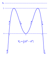
oscillates in the
potential between where
(20)
Stability of at time scales longer than the period of
oscillation is the time average of condition (19).
(21)
This is satisfied when is small.
When grows large enough that
condition (21) is violated,
the
solution becomes unstable.
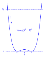
The Higgs field then starts down from the unstable equilibrium at
towards its
vacuum expectation value.
This is the beginning of the electroweak transition,
at scale factor where equality holds in
condition (21).
For an extremely rough estimate of the actual value of
suppose that the electroweak transition began at redshift
to within some orders of magnitude.
Suppose that the present scale factor is the Hubble time again to within some orders of magnitude.
Then is .
Combine this in (21) with
to get .
So the solutions that might be physically interesting will have
quite a large number, something like
and given by equality in (21) is
(22)
A complete analysis of the stability condition (17)
for all modes of the perturbation
is carried out in Note (1).
The result is that the zero-mode is the first mode to become unstable
as increases.
So equation (22) remains valid.
The oscillator is solved by integrating the energy
equation (11).
Change variables from , to ,
determines and vice versa,
so can be taken as the free parameter of the solution.
The cosmological gauge field is periodic
in imaginary proper time with period .
In co-moving time ,
given by so that the space-time metric is
,
the imaginary time period is .
The cosmological gauge field therefore acts as a thermal bath.
The period in imaginary co-moving time is
the inverse temperature,
At , the onset of the electroweak
transition, the temperature is
(33)
independent of the value of .
To solve the oscillator, let
(34)
The interesting values of are numbers , so
.
In dimensionless co-moving time , , the energy equation
(11) is
(35)
The solution is
(36)
with the relation to conformal time given by
(37)
The scale
factor ranges from to
as co-moving time ranges from to
and conformal time ranges from to
where .
The time scale of the oscillations
is much shorter than the expansion time scale, .
The next step
will be to find a classical solution for cosmology after the onset of the
electoweak transition, for .
The solution will include the gauge field along with the gauge field.
The gauge group will be .
In
the subgroup consisting of the with
acts on by
.
The symmetry group of the nonzero
Higgs field
is the subgroup
.
There should be a classical -symmetric solution describing the
descent of the Higgs field to its vacuum expectation
value.
Questions that will arise include: how much expansion will take place
during the descent? how much spatial anisotropy will be introduced?
will the cosmological gauge field violate CP symmetry during the
descent?
The temperature
suggests that is at redshift .
Considerable expansion will be needed during the electroweak
transition. The solution (36) for has an
inflationary epoch but
it does not set in until well after the
-symmetric solution becomes
unstable at .
The -symmetric solution will need to
spend some time in the inflationary neighborhood.
The -symmetric solution will be spatially homogeneous because
takes every point in to every other.
But the little group at a point in space is a
that leaves a preferred direction invariant.
The -symmetric solution will be anisotropic.
The question is how much anisotropy remains at large time.
The cosmological gauge field is -odd and -even
so it is -odd.
In the -symmetric solution
the oscillations are even in .
If the oscillations are critically damped or over-damped
in the solution, then
the very last
stage of the descent to 0 will break the
symmetry and thus break CP.
A second pressing task is to evaluate the corrections to the
-symmetric action due to thermal quantum fluctuations
of all the Standard Model fields
to check whether the classical -symmetric solution is materially affected.
The temperature is inversely proportional to
so there is a question
how far back before can the solution obtain before
corrections from unknown high energy physics become significant.
Eventually there will be the question of the origin of the
symmetry. Why should the gauge bundle
be isomorphic to
the spin bundle at early time? And why should be such a large
number?
The -symmetric classical cosmology is part of a project to
find a classical solution of the Standard Model combined with General
Relativity that is analytic in time and that captures the
observed macroscopic features of cosmology.
The project is an attempt at a top-down,
first-principles calculation of a complete macroscopic cosmology
within the Standard Model combined with General Relativity.
The hope is that the macroscopic classical cosmology
can be refined by microscopic corrections
into a quantitatively testable theory.
The first part of the project Friedan (2019) was an -symmetric classical solution
that captured some qualitative features of late-time cosmology:
a big bang followed by decelerating expansion followed by
accelerating expansion, driven by purely gravitational dark matter and
energy .
The hope is that the -symmetric solution will interpolate between the
-symmetric cosmology at early time and the
-symmetric cosmology at late time.
My particular agenda in this work
is to find evidence in support of a speculative fundamental theory of
physics in which the laws of physics are produced by the
2d renormalization group Friedan (2019).
In the pure gravity simplification of this theory,
the space-time metric is the coupling of a 2d quantum
field theory,
and the 2d rg drives to a
solution of .
This is an rg fixed point because the metric changes by
which is just an infinitesimal reparametrization of space-time.
The 2d rg fixed point equation is General Relativity
extended by the source term .
The source term provides dark matter and energy Friedan (2019).
In the full theory, the classical equations of motion of the
Standard Model combined with General Relativity are extended by source terms
corresponding to all the gauge symmetries of the theory.
The present work started out by
investigating the -symmetric equations of
motion with such source terms,
but the source terms turned out to be identically zero in the solution.
So the -symmetric solution
is presented here without connection to the 2d rg program
of Friedan (2019).
Later,
if a comprehensive macroscopic cosmology with the 2d rg source terms
can be derived successfully,
then global properties of the 2d rg flow
might be looked to for
explanation of early-time -symmetry
and the magnitude of the gauge field oscillations.
Acknowledgements.
This work was supported by the Rutgers New High Energy Theory Center
and by the generosity of B. Weeks.
I am grateful
to the Mathematics Division of the
Science Institute of the University of Iceland
for its hospitality.
Gradshteyn et al. (1996)I. Gradshteyn, A. Jeffrey,
and I. Ryzhik, Table of Integrals, Series, and
Products (Academic Press, 1996) sections 8.11, 8.14, 8.15.
(4)F. W. J. Olver et al., “NIST Digital Library of Mathematical Functions,” Release 1.0.26 of 2020-03-15, http://dlmf.nist.gov/, chapter 22 and section 19.2.