Finite-temperature spectroscopy of dirty helical Luttinger liquids

Abstract

We develop a theory of finite-temperature momentum-resolved tunneling spectroscopy (MRTS) for disordered, interacting two-dimensional topological-insulator edges. The MRTS complements conventional electrical transport measurement in characterizing the properties of the helical Luttinger liquid edges. Using standard bosonization technique, we study low-energy spectral function and the MRTS tunneling current, providing a detailed description controlled by disorder, interaction, and temperature, taking into account Rashba spin orbit coupling, interedge interaction and distinct edge velocities. Our theory provides a systematic description of the spectroscopic signals in the MRTS measurement and we hope will stimulate future experimental studies on the two-dimensional time-reversal invariant topological insulator.

I Introduction

Topology has become an important component of and has revolutionized modern condensed matter physics over the past few decades. Strikingly, topological condensed matter phenomena are robust to local heterogeneities (disorder), sample geometry, and other low-energy microscopic details. A paradigmatic example is the chiral edge state of the integer quantum Hall effect, which gives a quantized $e^{2}/h$ Hall conductance per channel, robust to local perturbations. Another significant advance is the prediction of a time-reversal (TR) symmetric topological insulators (TI) Kane and Mele (2005a, b); Bernevig and Zhang (2006); Hasan and Kane (2010); Qi and Zhang (2011) and more generally symmetry-protected TIs Senthil (2015), that stimulated numerous theoretical Xu and Moore (2006); Wu et al. (2006); Teo and Kane (2009); Maciejko et al. (2009); Schmidt et al. (2012); Väyrynen et al. (2013) and experimental investigations König et al. (2007); Knez et al. (2011); Suzuki et al. (2013); Du et al. (2015); Li et al. (2015); Qu et al. (2015); Ma et al. (2015); Nichele et al. (2016); Nguyen et al. (2016); Couëdo et al. (2016); Fei et al. (2017); Du et al. (2017); Li et al. (2017); Tang et al. (2017); Wu et al. (2018); Chen et al. (2018); Ugeda et al. (2018); Reis et al. (2017) (also see reviews and references therein, Hasan and Kane (2010); Qi and Zhang (2011); Dolcetto et al. (2015); Senthil (2015); Rachel (2018); Lunczer et al. (2019)).

A 2D time-reversal symmetric TI Kane and Mele (2005a, b); Bernevig and Zhang (2006) (of class AII Hasan and Kane (2010)) is a fully gapped bulk insulator with its edge hosting counter-propagating Kramers pairs of electrons. The time-reversal symmetric disorder cannot backscatter in the absence of interactions (though it can for an interacting edge, e.g., via a two-particle backscattering Wu et al. (2006); Xu and Moore (2006); Chou et al. (2018)) with edge electrons propagating ballistically, thus avoiding Anderson localization. Such ideal topologically protected helical Luttinger liquid (hLL) edge Wu et al. (2006); Xu and Moore (2006) is expected to exhibit a quantized $e^{2}/h$ zero-temperature conductance, controls the low-energy properties of the TI, and provides a new platform for studying and testing the low-energy Luttinger liquid (LL) theory of interacting one-dimensional electronic systems.

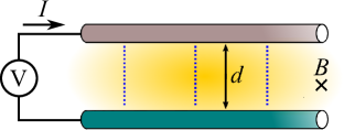
Figure 1: A schematic of an experimental setup for momentum-resolved tunneling spectroscopy, with dashed lines indicating the single particle tunneling between two separated topological insulator edges, and momentum transfer tuned with an out-of-plane magnetic field applied to the yellow shaded region.

In contrast to the quantum Hall edges, a transport in 2D TR symmetric TI edges is sensitive to a set of microscopic details. At the simplest level a hLL is predicted to exhibit interaction strength-dependent power-laws in frequency, voltage and temperature Maciejko et al. (2009); Tanaka et al. (2011); Lezmy et al. (2012); Kainaris et al. (2014); Chou et al. (2015). In a more detailed analysis, the primary finite-temperature conductance correction is believed to come from charge puddles near the edge Väyrynen et al. (2013, 2014). The charge puddles can behave like Kondo impurities Väyrynen et al. (2014); Maciejko et al. (2009); Tanaka et al. (2011) and can generate insulator-like finite-temperature conductivity Väyrynen et al. (2016). External noise Väyrynen et al. (2018) and intraedge inelastic interaction Maciejko et al. (2009); Schmidt et al. (2012); Kainaris et al. (2014); Chou et al. (2015) are also predicted to give nontrivial conductance corrections. To our knowledge, however, the existing experiments have not systematically demonstrated the finite-temperature conductivity predicted by any of the above theories. Among various other potential explanations (see e.g., Pikulin et al. (2014); Hu et al. (2016); Li et al. (2018); Skolasinski et al. (2018); Chou et al. (2018); Novelli et al. (2019)) is a novel spontaneous symmetry-breaking localization due to an interplay of TR symmetric disorder and interaction Chou et al. (2018), in contrast to Anderson localization due to a magnetic ordering of an extensive number of the Kondo impurities Altshuler et al. (2013); Hsu et al. (2017). Generally, one expects that disorder with weak interactions does not modify the edge state dc conductance Kane and Mele (2005b); Xie et al. (2016). In light of above puzzling transport measurements, an independent experimental probe of the helical Luttinger liquid (hLL) edges is highly desirable.

In the present study, we calculate a spectral function of a disordered, finite-temperature hLL, and based on it develop a theory of the finite-temperature momentum-resolved tunneling spectroscopy (MRTS) Auslaender et al. (2002); Steinberg et al. (2008); Jompol et al. (2009); Tsyplyatyev et al. (2015, 2016); Jin et al. (2019) between two (TR symmetrically) disordered, interacting TI helical edges. Such MRTS setup thereby provides an independent spectral characterization of the hLLs, complementary to conventional transport. In contrast to earlier work Braunecker and Simon (2018), which focused on clean short zero-temperature hLLs, we study disordered interacting long TI edges at finite temperatures. In the absence of interedge interaction, the tunneling current spectroscopy is simply related to a convolution of two fermionic edge spectral functions, that we compute in a detailed closed form. An interedge interaction requires a nonperturbative treatment. Utilizing bosonization, perturbatively in the tunneling we derive the disorder-averaged, finite temperature MRTS tunneling current, that depends sensitively on mismatch of edge velocities. In contrast to conventional LL edges Carpentier et al. (2002), TR symmetric disorder does not back-scatter helical edge electrons. Thus our low-energy analysis makes predictions that are nonperturbative in interaction and disorder, providing a detailed characterization of a hLL that should be experimentally accessible.

Before delving into details of the analysis, we summarize our results in Sec. II. Then, in Sec. III, utilizing bosonization we study the finite-temperature spectral function of a helical edge of a TR invariant TI in the presence of symmetry-preserving disorder and interactions. In Sec. IV, building on the single-edge analysis we study the interedge tunneling, showing that it can be used as a momentum-resolved spectroscopic probe of helical edges, with momentum and frequency tuned by an external magnetic field and interedge voltage, respectively, as illustrated in Fig. 1. We conclude in Sec. V with a discussion of using this momentum-resolved tunneling spectroscopy to unambiguously experimentally identify TI edges, that have resisted clear identification in a conventional transport measurements. We relegate much of our somewhat technical analysis to numerous appendices.

II Summary of main results

We briefly summarize the key results of our study, detailed in subsequent sections of the manuscript. Utilizing bosonization we studied finite temperature spectral properties of an interacting helical edge of a TR invariant TI in the presence of symmetry-preserving disorder. Although a number of similar analyses have appeared in the literature Luther and Peschel (1974); Meden and Schönhammer (1992); Voit (1993); Orgad (2001), to the best of our knowledge our computation is the most detailed and complete at finite temperature. Inside the hLL phase Wu et al. (2006); Xu and Moore (2006); Chou et al. (2018), the edge is fully characterized by a Luttinger parameter $K$ and exponent $\gamma\equiv\frac{1}{4}\left(K+K^{-1}\right)-\frac{1}{2}$, with $K=1$ ($\gamma=0$) in a non-interacting limit and $K<1$ ($\gamma>0$) for repulsive interaction.

We derive a detailed expression for the disorder-averaged, low-temperature spectral function Eq. (36), that in the limit of strong disorder $\Delta$ is given by

$$A(\omega,q)\approx T^{2\gamma}\frac{\xi/\pi}{(q\xi)^{2}+1}f_{\gamma}\left(\frac{\omega}{T}\right),$$ (1)

where $\xi=2v^{2}/K^{2}\Delta$ is a disorder length scale, $v$ is the edge velocity and $T$ is temperature (with $\beta=T^{-1}$ the inverse temperature). For convenience, we set ${\hbar=k_{B}=1}$ throughout this paper. Above,

$$f_{\gamma}\left(x\right)\sim\left\{\begin{array}[]{cc}x^{2\gamma},&\text{ for }x\gg 1\\ 1,&\text{ for }x\ll 1\end{array}\right.$$ (4)

is a scaling function, with the exact form given by the Euler Beta function derived in the main text, Eq. (34). The complete expression for a right-mover $A(\omega,q)$, characterized by a broad peak at $\omega=vq$ and a zero-bias anomaly at $\omega=0$, is illustrated for a set of temperatures in Fig. 2. The broadening of the quasiparticle peak is described by the full width at half maximum (FWHM) $4\pi\gamma T+2v\xi^{-1}$, which suggests that a probe of the momentum-resolved spectral function can be used to quantify the interaction and (forward-scattering) disorder strength.

We note that although generically one expects sample heterogeneity to smear out sharp features of a clean system, here disorder average of the finite-momentum spectral function, $A(\omega,q)$ brings out the sharp zero-bias anomaly that is otherwise absent at finite momentum. This counter-intuitive effect arises due to impurities providing the momentum needed to shift the $q=0$ zero-frequency anomaly to a finite momentum $q$, as shown in Fig. 2. All figures in this paper are plotted in the units of $v\alpha^{-1}$ and $\alpha$ for frequency and length respectively, where $\alpha$ is the ultraviolet cutoff length scale in LL theory.

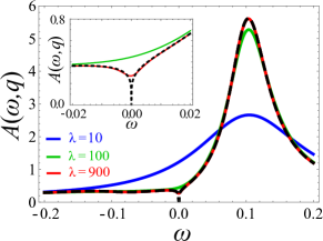
Figure 2: Single helical edge, disorder-averaged spectral function, illustrated for a set of temperatures (characterized by a thermal length $\lambda=v\beta$), disorder length $\xi=30$, $vq=0.1$, and interaction parameter $\gamma\equiv\frac{1}{4}\left(K+K^{-1}\right)-\frac{1}{2}$ taken to be $0.1$. The black dashed line denotes the zero temperature ($\lambda=\infty$) spectral function. The inset shows the details of thermal rounding of the zero-bias anomaly. The frequency and the length are in units of $v\alpha^{-1}$ and $\alpha$ respectively.

Our second key prediction is that of the finite-temperature momentum-resolved interedge tunneling current $J(\omega=eV/\hbar,Q=2\pi Bd/\phi_{0})$ in the presence of disorder and interaction, and tunable by an external magnetic field $B$ and voltage bias $V$, as illustrated in a schematic setup of Fig. 1. In the above, $d$ denotes the distance between two edges and $\phi_{0}=h/e$ is the magnetic flux quantum. Importantly, $Q$ is the momentum shift between the energy bands of the two edges controlled by the external magnetic field. The representative predictions for the tunneling current, computed perturbatively in the tunneling are given by the following analytical expressions. For the vertical geometry (Fig. 10) with identical edges (same velocity and interaction but different Fermi wavevectors $k_{F,1}\neq k_{F,2}$), the tunneling current in the absence of disorder and interedge interaction is well approximated by $J_{RR}(\omega,Q+k_{F,1}-k_{F,2})+J_{LL}(\omega,Q-k_{F,1}+k_{F,2})$, where

$$J_{LL}(\omega,q) =-2et_{0}^{2}\left(\frac{2\pi\alpha}{\beta v}\right)^{4\gamma}\frac{1}{4\pi^{2}v}\sin(2\pi\gamma)$$

$$\quad\,\times\text{Im}\left\{B\left[\frac{\beta(-i\omega+ivq)}{4\pi}+\gamma+1,-1-2\gamma\right]\right.$$

$$\quad\quad\,\,\times\left.B\left[\frac{\beta(-i\omega-ivq)}{4\pi}+\gamma,1-2\gamma\right]\right\},$$ (5)

and $J_{RR}(\omega,q)=J_{LL}(\omega,-q)$. For the horizontal geometry (Fig. 16) with identical edges, the tunneling current is given by $J_{RL}(\omega,Q+k_{F,1}+k_{F,2})+J_{LR}(\omega,Q-k_{F,1}-k_{F,2})$ where

$$J_{RL/LR}(\omega,q) =-2et_{0}^{2}\left(\frac{2\pi\alpha}{\beta v}\right)^{4\gamma}\frac{1}{4\pi^{2}v}\sin(2\pi\gamma)$$

$$\quad\,\times\text{Im}\left\{B\left[\frac{\beta(-i\omega+ivq)}{4\pi}+\gamma+\frac{1}{2},-2\gamma\right]\right.$$

$$\quad\quad\,\,\times\left.B\left[\frac{\beta(-i\omega-ivq)}{4\pi}+\gamma+\frac{1}{2},-2\gamma\right]\right\}.$$ (6)

The effects of forward-scattering disorder can be included through a convolution with a Lorentzian (with width $\xi^{-1}$, where $\xi$ is the disorder length). With Eqs. (5) and (6), the differential tunneling conductance can be derived. The differential tunneling conductance for both vertical and horizontal geometries are plotted in Fig. 3. We discuss the more generic case (e.g., including interedge interaction, distinct edge velocities, etc) in Sec IV.

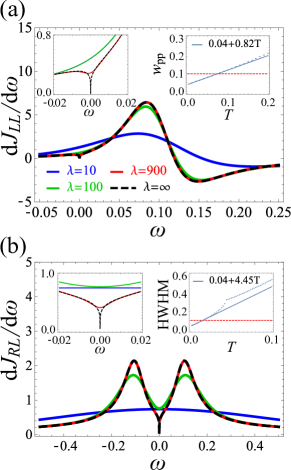
Figure 3: Finite-temperature differential tunneling conductance $dJ(\omega=eV/\hbar,Q=2\pi Bd/\phi_{0})/d\omega$ in the presence of forward-scattering disorders (with disorder length $\xi=20$) around (a) two left Fermi points and (b) right and left Fermi points, illustrated for a range of temperatures characterized by the thermal length $\lambda=v\beta$. Velocity and interaction are taken to be identical for the two edges, with the more generic expression given in the main text. The interaction parameter $\gamma\equiv\frac{1}{4}\left(K+K^{-1}\right)-\frac{1}{2}$ is taken to be $0.05$ and $vq=-0.1$. The left inset is the magnification of the zero-bias anomaly. The right insets show linear temperature dependence of (a) the distance (in $\omega$) between the left-positive and right-negative peaks ($w_{pp}$) and (b) the half width at half maximum (HWHM) respectively for $T<|vq|$ (red dashed lines). The frequency and the length are in units of $v\alpha^{-1}$ and $\alpha$ respectively.

A map of tunneling current can be constructed by tuning $B$ and $V$ independently. In the absence of the interaction, the tunneling currents are nonzero only in the kinematically allowed regions Carpentier et al. (2002) illustrated in Fig. 4. The interactions modify the kinematically allowed region as we discuss in the main text.

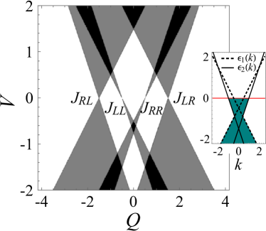
Figure 4: Schematic diagram of momentum-resolved tunneling current for two non-interacting TI edges. There are four tunneling regions (gray color, labeled by $J_{\alpha\alpha^{\prime}}$) for low bias $V\approx 0$, corresponding to tunneling between $\alpha$ (of edge 1) and $\alpha^{\prime}$ (of edge 2) Fermi points. The current flows from edge 1 to 2 (positive current) and from edge 2 to 1 (negative current) for positive and negative bias voltages respectively. The black regions indicate that tunneling happens between two pairs of Fermi points. Inset: energy bands of edge 1 (dashed line) and edge 2 (solid line) used for generating the main figure. The red line denotes the Fermi energy at equilibrium ($V=0$).

We now turn to the detailed analysis that leads to the above results, as well as exploration of a number of different parameters and experimental geometries.

III Single edge: Model and spectral function

The edge states of a two-dimensional time-reversal symmetric topological insulator exhibit counterpropagating fermion Kramers pair. In contrast to a conventional Luttinger liquid, the TR symmetry on the edge constrains relevant interactions and disorder perturbatons to be forward-scattering only. The absence of Anderson localization is the manifestation of the topological protection of the TI edges. The gapless insulating localized states can still appear through spontaneous TR symmetry breaking for $K<3/8$ Wu et al. (2006); Xu and Moore (2006) due to an interplay of interaction and disorder Chou et al. (2018). In this work, we exclusively focus on the $K>3/8$ hLL phase. We next introduce the minimal model for such disordered hLL and then study its finite-temperature spectral function using bosonization Shankar (2017); Giamarchi (2004).

III.1 Weakly interacting generic hLL

A helical edge is characterized by a Kramers pair of right-moving, $c_{+}(k)$ and left-moving, $c_{-}(k)$ fermions at each quasi-momentum $k$. Under antiunitary TR operation $\mathcal{T}$, the TR symmetric partners are related to each other by $\mathcal{T}c_{\pm}(k)\mathcal{T}^{-1}=\pm c_{\mp}(-k)$ ($\mathcal{T}^{2}=-1$). To describe low energy physics around Fermi points $\pm k_{F}$, the field operators can be expressed in terms of the slowly-varying fermionic degrees of freedom $R$ and $L$ near $k_{F}$ and $-k_{F}$, respectively,

$$c_{+}(x)= \int\frac{dk}{2\pi}\,e^{ikx}c_{+}(k)\approx e^{ik_{F}x}R(x)$$

$$c_{-}(x)= \int\frac{dk}{2\pi}\,e^{ikx}c_{-}(k)\approx e^{-ik_{F}x}L(x).$$ (7)

In TI samples without mirror symmetry, the Rashba spin-orbit coupling (RSOC) is generically present. The primary effect of the RSOC is to induce momentum-dependent spin rotation Schmidt et al. (2012); Rod et al. (2015). As a result, the field operators with a definite spin projection $\uparrow$ and $\downarrow$ are a linear combination of chiral fields Xie et al. (2016) (also see Appendix A for a derivation),

$$c_{\uparrow}(x)\approx e^{ik_{F}x}R(x)-i\zeta e^{-ik_{F}x}\partial_{x}L(x)$$

$$c_{\downarrow}(x)\approx e^{-ik_{F}x}L(x)-i\zeta^{*}e^{ik_{F}x}\partial_{x}R(x),$$ (8)

where length $\zeta$ encodes the degree of “spin rotation texture”. In a simple model discussed in Schmidt et al. (2012), $\zeta=2k_{F}/k_{0}^{2}$, where $k_{0}$ characterizes the strength of RSOC. In Eq. (III.1), the spin quantization axis is chosen such that $\uparrow$ and $\downarrow$ match the spins at Fermi points $\pm k_{F}$ respectively. Next, we construct the low-energy Hamiltonian for the helical edge.

The kinetic part of the Hamiltonian is given by

$$H_{\text{0}} =v_{F}\int dx\left[R^{\dagger}\left(-i\partial_{x}R\right)-L^{\dagger}\left(-i\partial_{x}L\right)\right]$$ (9)

where $v_{F}$ is the Fermi velocity. The interaction and disorder parts of the Hamiltonian couple to the electron density, given by

$$\rho(x)= R^{\dagger}R+L^{\dagger}L$$

$$-\left\{i\zeta e^{-i2k_{F}x}\left[R^{\dagger}(\partial_{x}L)-(\partial_{x}R^{\dagger})L\right]+\text{H.c.}\right\},$$ (10)

where only terms up to $O(\zeta)$ are kept. The low-energy expansion of the electron density contains a slowly-varying (low momentum transfer) and a fast-varying ($2k_{F}$ momentum transfer) contributions. It is important to note that Eq. (10) is invariant under TR operation ($R\rightarrow L$, $L\rightarrow-R$, and $i\rightarrow-i$).

It is instructive to consider a chemical potential shift coupled to the density, $\rho(x)$ given by (10) in the presence of RSOC. The key observation is that the shifted Hamiltonian can be brought back to the original gapless form (9)

$$H_{0}^{\prime}\equiv H_{0}-\delta\mu\int dx\,\rho(x)$$ (11)

$$= v_{F}^{\prime}\int dx\left[R^{\prime\dagger}\left(-i\partial_{x}R^{\prime}\right)-L^{\prime\dagger}\left(-i\partial_{x}L^{\prime}\right)\right],$$ (12)

with $k_{F}$-dependent rotation of the quantization axis of the helical fermions,

$$\left[\begin{array}[]{c}R^{\prime}(x)\\ L^{\prime}(x)\end{array}\right]=e^{-i\hat{\sigma}_{z}k_{F}^{\prime}x}e^{-i\hat{\sigma}_{y}\theta/2}e^{i\hat{\sigma}_{z}k_{F}x}\left[\begin{array}[]{c}R(x)\\ L(x)\end{array}\right],$$ (17)

characterized by $\theta=\tan^{-1}\left(2\delta\mu\,\zeta/v_{F}\right)$, $k_{F}^{\prime}=\frac{v_{F}k_{F}+\delta\mu}{v_{F}^{\prime}}$, and $v_{F}^{\prime}=\sqrt{v_{F}^{2}+\left(2\delta\mu\,\zeta\right)^{2}}$ (to simplify the expression we have taken $\zeta$ to be real). The gapless helical edge remains topologically protected against uniform RSOC as long as the bulk gap is finite Kane and Mele (2005a).

The key qualitative distinguishing feature of hLL is that TR invariance forbids Anderson localization of the edge Kramers pairs by nonmagnetic impurities. In the absence of RSOC this is manifest as the density operator, $R^{\dagger}R+L^{\dagger}L$ is only forward-scattering. In the presence of both RSOC and the TR symmetric disorder, a position-dependent rotation can again map the theory to the 1D massless Dirac Hamiltonian in a fixed realization of disorder Xie et al. (2016). Thus, low-energy effects of TR invariant disorder on the helical edges of a TI are qualitatively captured by random forward scattering perturbation,

$$H_{\text{dis}}= \int dx\,V(x)\left[R^{\dagger}R+L^{\dagger}L\right].$$ (18)

Without loss of generality, we take the random potential $V(x)$ to have zero-mean and Gaussian statistics characterized by disorder average

$$\overline{V(x)V(y)}=\Delta\delta(x-y),$$ (19)

with variance amplitude, $\Delta$.

Within the stable hLL phase, the interaction is dominated by forward-scattering, given by

$$H_{\text{int}}= \int\limits_{x}:\left[UR^{\dagger}R(x+\alpha)R^{\dagger}R(x)\right.$$

$$+ U^{\prime}\left.R^{\dagger}R(x+\alpha)L^{\dagger}L(x)+(R\to L):\right]$$ (20)

where $U$ and $U^{\prime}$ are the screened short-range components of Coulomb interaction and $\alpha$ is the ultraviolet cutoff length scale. We neglect the backscattering components (in the presence of RSOC) Schmidt et al. (2012); Kainaris et al. (2014); Chou et al. (2015) since they are subdominant in the regime studied in this work.

The Hamiltonian $H_{\text{hLL}}=H_{\text{0}}+H_{\text{int}}+H_{\text{dis}}$ given by Eqs. (9), (18), and (III.1) is the minimal model of the interacting, dirty helical edge of a topological insulator protected by TR symmetry. As we will see next, the model is exactly solvable by bosonization, allowing a nonperturbative description of TI’s helical edge.

III.2 Bosonization

To treat Luttinger interaction and disorder, $H_{\text{int}}+H_{\text{dis}}$ nonperturbatively we utilize a standard bosonization analysis Shankar (2017); Giamarchi (2004), summarized in Appendix B. Using the imaginary-time path-integral formalism, the disordered helical Luttinger liquid is characterized by the imaginary-time action, $\mathcal{S}=\mathcal{S}_{\text{hLL}}+\mathcal{S}_{\text{dis}}$, where

$$\mathcal{S}_{\text{hLL}}= \int\limits_{\tau,x}\left\{\frac{i}{\pi}\left(\partial_{x}\theta\right)\left(\partial_{\tau}\phi\right)+\frac{v}{2\pi}\left[K\left(\partial_{x}\phi\right)^{2}+\frac{1}{K}\left(\partial_{x}\theta\right)^{2}\right]\right\},$$ (21)

$$\mathcal{S}_{\text{dis}}= \int\limits_{\tau,x}V(x)\frac{1}{\pi}\partial_{x}\theta,$$ (22)

with $\theta$ the phonon-like boson field and $\phi$ the phase boson field. The number density and number current operators are given by $\rho=\frac{1}{\pi}\partial_{x}\theta$ and $J=-\frac{1}{\pi}\partial_{t}\theta$, respectively. Although the action $S_{\text{hLL}}$ takes the form of a conventional spinless Luttinger liquid (LL) Giamarchi (2004), the physics of this helical LL differs significantly because of distinct TR transformations of $\theta$ and $\phi$ here, due to nontrivial spin content of the corresponding helical edge fermions (see Appendix B). As noted above this latter property has important physical manifestations, as for example forbidding potential impurity backscattering in the absence of umklapp interactions.

We note that the forward-only scattering disorder, can be fully non-perturbatively taken into account by shifting $V(x)$ from the action via a linear transformation on $\theta$, $\mathcal{S}_{\text{hLL}}[\theta,\phi]+\mathcal{S}_{\text{dis}}[\theta]\rightarrow\mathcal{S}_{\text{hLL}}[\tilde{\theta},\phi]+\text{constant}$, where

$$\tilde{\theta}(\tau,x)=\theta(\tau,x)+\frac{K}{v}\int_{-\infty}^{x}V(y)dy.$$ (23)

Under this shift, the correlation functions of $\theta$ transform covariantly. For instance,

$$\left\langle e^{-in\theta(\tau,x)}e^{in\theta(0,0)}\right\rangle=e^{-i\frac{nK}{v}\int_{0}^{x}V(y)dy}\left\langle e^{-in\tilde{\theta}(\tau,x)}e^{in\tilde{\theta}(0,0)}\right\rangle,$$ (24)

shifts by a $V(x)$-dependent phase factor, that now allows for an exact disorder average of the correlation function. In the above, $n$ is a constant controlling the scaling dimension of the operator. Gaussian statistics of $V(x)$, with variance (19) then gives

$$\overline{\left\langle e^{-in\theta(\tau,x)}e^{in\theta(0,0)}\right\rangle}=e^{-\frac{n^{2}K^{2}\Delta}{2v^{2}}|x|}\left\langle e^{-in\tilde{\theta}(\tau,x)}e^{in\tilde{\theta}(0,0)}\right\rangle.$$ (25)

Forward-scattering disorder thus suppresses power-law Luttinger liquid correlations, cutting them off exponentially beyond a correlation length $\xi=2v^{2}/(n^{2}K^{2}\Delta)$, that in momentum space corresponds to smearing the disorder-free power-law peak via a convolution with a Lorentzian, with width set by $1/\xi$.

III.3 Spectral function

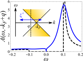
Figure 5: Zero-temperature spectral function along the cut through $k=-k_{F}+q$ indicated by a dashed line in the inset with full (dashed) curve for disordered (clean) case. The interaction parameter $\gamma\equiv\frac{1}{4}\left(K+K^{-1}\right)-\frac{1}{2}$ is set to 0.1. Inset: The spectral function in the vicinity of the left Fermi point. The yellow shaded region indicates finite weight of the clean spectral function. The width of the blue double arrow is the inverse length scale ($\xi^{-1}$) set by the strength of forward-scattering disorder.

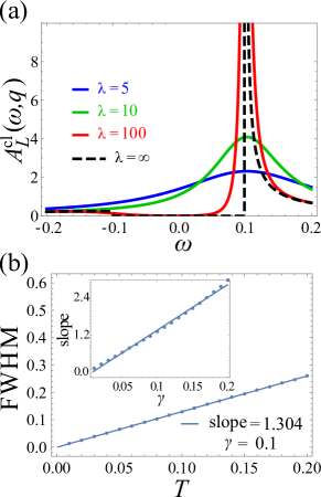
Figure 6: Finite-temperature clean (disorder-free) spectral function for a set of temperatures characterized by thermal de Broglie length, $\lambda=v\beta$. (a) The interaction parameter $\gamma=0.1$ and $vq=-0.1$. (b) Quasiparticle peak width as a function of temperature $T$ and $\gamma$. The linear dependence on $T$ and $\gamma$ shows $\text{FWHM}\approx 4\pi\gamma T$. The frequency and the length are in units of $v\alpha^{-1}$ and $\alpha$ respectively.

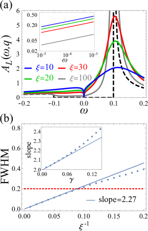
Figure 7: Zero-temperature spectral function with forward-scattering disorder. The interaction parameter $\gamma=0.1$ and $vq=-0.1$. (a) Zero bias anomaly (ZBA) appears at $\omega=0$ for all disorder strengths $\xi^{-1}$, with the same exponent $2\gamma$ (inset), where $\xi=\frac{2v^{2}}{K^{2}\Delta}$. (b) The quasiparticle peak is broadened by disorders with a (half) width $~{}\xi^{-1}$ for $\text{FWHM}<|vq|$ (dashed red line), beyond which ZBA modifies the linear dependence. Inset: The slope $=2$ in the noninteracting limit and the disorder-strength dependence becomes more sensitive for stronger interaction. The frequency and the length are in units of $v\alpha^{-1}$ and $\alpha$ respectively.

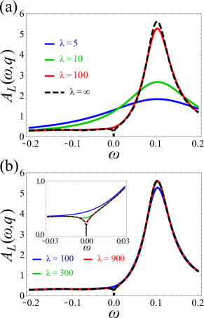
Figure 8: Finite-temperature spectral function with forward-scattering disorder. (a) High temperature regime $\lambda\ll\xi$. (b) Low temperature regime $\lambda\gg\xi$. The disorder length $\xi=30$, the interaction parameter $\gamma=0.1$ and $vq=-0.1$. The frequency and the length are in units of $v\alpha^{-1}$ and $\alpha$ respectively.

III.3.1 Clean spectral function

In the clean limit, the imaginary time-ordered, single particle space-time Green function at finite temperature is well-known for a spinless LL Giamarchi (2004). Although physically hLL and LL are quite distinct, because the actions of the two systems are identical at a leading order, we find that the single-edge spectral function for a hLL is identical to that of a spinless LL. The calculation can be carried out at zero temperature followed by a conformal mapping [a mapping from a $(\tau,x)$ 2D plane to a cylinder in the space-imaginary time domain] to get the finite temperature expression. The finite temperature Green function can be also obtained directly through the Matsubara technique. We provide a complemented derivation using the latter approach in Appendix C. Both analyses consistently give the single particle imaginary time-ordered Green function for the right and left movers,

$$\mathcal{G}_{R}(\tau,x)=-\langle\hat{T}_{\tau}R(\tau,x)R^{{\dagger}}(0,0)\rangle$$

$$=-\frac{i}{2\pi\alpha}\frac{(\frac{\pi\alpha}{\beta v})^{2\gamma+1}}{\left[\sinh\left(\frac{\pi(x+iv\tau)}{\beta v}\right)\right]^{\gamma+1}\left[\sinh\left(\frac{\pi(x-iv\tau)}{\beta v}\right)\right]^{\gamma}}$$ (26)

$$\mathcal{G}_{L}(\tau,x)=-\langle\hat{T}_{\tau}L(\tau,x)L^{{\dagger}}(0,0)\rangle$$

$$=\frac{i}{2\pi\alpha}\frac{(\frac{\pi\alpha}{\beta v})^{2\gamma+1}}{\left[\sinh\left(\frac{\pi(x+iv\tau)}{\beta v}\right)\right]^{\gamma}\left[\sinh\left(\frac{\pi(x-iv\tau)}{\beta v}\right)\right]^{\gamma+1}},$$ (27)

where $\alpha$ is the ultraviolet cutoff length scale, $\gamma=\frac{1}{4}(K+K^{-1})-\frac{1}{2}$ and $\hat{T}_{\tau}$ denotes imaginary-time ordering. The spectral function can be computed in the standard way by Fourier transforming the imaginary time-ordered Green function $\mathcal{G}_{R/L}(\tau,x)$ and then analytically continuing to real frequencies $i\omega_{n}\to\omega+i\eta$, where $\eta\rightarrow 0^{+}$. The disorder-free (“clean”) spectral function $A^{\text{cl}}(\omega,q)$ is then given by

$$A^{\text{cl}}_{R/L}(\omega,q)=-\frac{1}{\pi}\text{Im}[G^{\text{ret}}_{R/L}(\omega,q)],$$ (28)

where the retarded Green function $G^{\text{ret}}_{R/L}(\omega,q)$ is computed using standard analysis, detailed in Appendix D,

$$G^{\text{ret}}_{R/L}(\omega,q)= i\frac{\beta(\frac{2\pi\alpha}{\beta v})^{2\gamma}}{4\pi^{2}}\sin\left(\pi\gamma\right)$$

$$\times B\left[-i\frac{\beta(\omega_{\eta}\mp vq)}{4\pi}+\frac{\gamma}{2},1-\gamma\right]$$

$$\times B\left[-i\frac{\beta(\omega_{\eta}\pm vq)}{4\pi}+\frac{\gamma+1}{2},-\gamma\right]$$ (29)

with $q=k\mp k_{F}$ for the right (subscript $R$) and left (subscript $L$) movers, respectively. In Eq. (III.3.1), $B$ is the Euler Beta function and $\omega_{\eta}\equiv\omega+i0^{+}$. To the best of our knowledge, the full expression of $G^{\text{ret}}_{R/L}(\omega,q)$ has not appeared in the literature, with only the imaginary part (or the greater/lesser Green functions) given in Ref. Orgad (2001). A few remarks of our results: (i) In doing Fourier transformation, we consider the approximate space-time Green function valid for $v\tau,x>\alpha$, (ii) The zero temperature limit of Eq. (III.3.1) is in good agreement with the result in Ref. Meden and Schönhammer (1992) (both real and imaginary parts) for $\gamma<0.5$ at low energy $\omega/v,q<1/\alpha$, (iii) The finite temperature spectral function derived from Eq. (III.3.1) is consistent with the result in Ref. Orgad (2001), (iv) Our expression satisfies the Kramers-Kronig relation for $\gamma<0.5$.

We first discuss the clean spectral function. At zero temperature, the spectral weight is constrained within the “light cone” [the yellow shaded region in the inset of Fig. 5]. The quasiparticle peak is a power-law singularity located at $\omega=-vq$ for the left mover, and at $\omega=vq$ for the right mover, with the exponent $\gamma=\frac{1}{4}(K+K^{-1})-\frac{1}{2}$, as illustrated in Fig. 5 Luther and Peschel (1974); Meden and Schönhammer (1992); Voit (1993, 1995). We plot in Fig. 6(a) the non-zero temperature, disorder-free (left) spectral function for different values of thermal length $\lambda=v\beta$ and $vq=-0.1$, illustrating thermal broadening of the “light cone” constraint. Throughout this paper, we plot the spectral function (and the momentum-resolved tunneling spectroscopy in the next section) in the low energy regime $\omega/v,q<\alpha^{-1}$ (note $\alpha=1$), where our low-energy Hamiltonian is valid.

The power-law threshold singularity is smeared at finite temperature, displaying low temperature $\lambda^{-1}\ll|q|$ (quantum) and high temperature $\lambda^{-1}\gg|q|$ (classical) regimes. For the former, the quasiparticle peak remains asymmetric, while for the latter, the smeared peak approaches a Lorentzian at high temperature. The broadening of the peak is nicely captured by a $2\pi\gamma T$ inelastic rate as discussed by Le Hur Le Hur (2002, 2006). We note that the linear in $T$ and $\gamma$ broadening is very robust starting from low temperature until $T$ becomes comparable to the ultraviolet cutoff, as illustrated in Fig. 6(b).

The features discussed above can be understood in the following. The Beta functions in the exact expression (III.3.1) can be expressed through an integral identity,

$$B\left(-i\frac{\kappa}{2}+\frac{C}{2},1-C\right) =2\int_{0}^{\infty}d\xi e^{i\kappa\xi}\left(2\sinh\xi\right)^{-C},$$ (30)

which gives the retarded Green function expressed as integrals over the light-cone coordinates $\xi_{\pm}=vt\pm x$ $(\tau\sim it)$

$$G^{\text{ret}}_{R/L}(\omega,q)= \frac{i}{2\beta v^{2}}\sin\left(\pi\gamma\right)(\frac{\pi\alpha}{\beta v})^{2\gamma}$$

$$\times\int_{0}^{\infty}d\xi_{\pm}e^{i(\omega\mp vq)\xi_{\pm}/2v}\sinh\left(\frac{\pi\xi_{\pm}}{\beta v}\right)^{-\gamma}$$

$$\times\int_{0}^{\infty}d\xi_{\mp}e^{i(\omega\pm vq)\xi_{\mp}/2v}\sinh\left(\frac{\pi\xi_{\mp}}{\beta v}\right)^{-\gamma-1}.$$ (31)

The low-temperature ($\omega\mp vq\gg\frac{1}{\beta}$) power-law and high-temperature ($\omega\mp vq\ll\frac{1}{\beta}$) Lorentzian forms of the quasiparticle peak respectively correspond to the two different limits of integral representation in Eq. (30): $\sinh(x)\approx x$ for $|x|\ll 1$ and $\sinh(x)\approx\operatorname{sgn}(x)e^{-|x|}/2$ for $|x|\gg 1$.

III.3.2 Disorder-averaged spectral function

In the presence of disorder, the momentum is no longer a good quantum number. However, generic spectroscopic experiments probe the disorder-averaged spectral function, analysis of which we discuss next. As emphasized in Sec. III, TR invariance constrains heterogeneities to nonmagnetic impurities that can only forward-scatter. The resulting disorder can thus be treated exactly and in real space is given by Eq. (25). In momentum space, disorder thus smears the disorder-free spectral function through its convolution with a Lorentzian, and is given by,

$$\overline{A_{R/L}(\omega,q)}= \int_{-\infty}^{\infty}dk\frac{\xi^{-1}/\pi}{(k-q)^{2}+\xi^{-2}}A^{\text{cl}}_{R/L}(\omega,k),$$ (32)

illustrated in Fig. 5, where $\xi=\frac{2v^{2}}{K^{2}\Delta}$ is the mean-free path set by the forward-scattering disorder. Despite this expected smearing of sharp features by disorder, we observe that disorder-averaged spectral function, $\overline{A_{R/L}(\omega,q)}$, illustrated in Fig. 7(a) in fact exhibits (even at finite momentum $q$) a disorder-induced zero-bias anomaly (ZBA), $\overline{A_{R/L}(\omega,q)}\propto\mathcal{C}|\omega|^{2\gamma}$ Giamarchi (2004), with exponent $\gamma$ and amplitude $\mathcal{C}=\frac{1}{\pi^{2}v}\sin\left(2\pi\gamma\right)|\Gamma(-2\gamma)|(\frac{\alpha}{v})^{2\gamma}\frac{\xi^{-1}}{q^{2}+\xi^{-2}}$, that is independent of disorder strength. The origin of this finite $q$ ZBA is most transparent in the strong disorder limit ($\xi q\ll 1$), where we can approximate the Lorentzian in Eq. (32) simply by a constant $\xi/\pi$, with the convolution thereby reducing to an integral over $k$, giving a local density of states, which is known to exhibit a ZBA Giamarchi (2004). Physically, this counter-intuitive effect is due to impurities providing the momentum needed to shift the $q=0$ zero-frequency anomaly to a finite momentum $q$.

In contrast, the power-law peak at $\omega=vq$ is indeed broadened by disorder, with the width $\propto K^{2}\Delta/v$, decreasing with stronger repulsive interactions, in contrast to thermal effects in disorder-free system discussed above [see Fig. 7(b)].

In the presence of both finite temperature and disorder one expects a broadening of the disorder-free, zero-temperature spectral function. Indeed we find that at high temperature, such that $\lambda\ll\xi$, the broadening of the quasiparticle peak is dominated by thermal effect, with spectral function reducing to the finite $T$ clean case [see Fig. 8(a)]. In particular, the quasiparticle peak approaches a Lorentzian with a (half) width $\approx 2\pi\gamma T+v\xi^{-1}$, corresponding to temporal exponential decay rate of the momentum-time Green function [read by a replacement $\tau\to it$ and $x\to-vt$ in Eq. (27)] Le Hur (2006) at high temperature. As we will show below, the prediction of the peak width in the high temperature limit works surprisingly well even at low temperature.

Instead, at low temperatures, such that $\lambda\gg\xi$, the spectral peak broadening is dominated by disorder as is clearly reflected in Fig. 8(b). We note the ZBA at $\omega=0$ is thermally rounded for $\omega\ll\omega^{*}(T)=v/\lambda\approx T$. This can be understood in the following way: the disorder-induced exponential decay results in an effective constraint $|x|=|\xi_{+}-\xi_{-}|/2\approx 0$ in Eq. (31), giving

$$G^{\text{ret}}_{\text{dis},R(L)}(\omega,q)\approx \frac{i}{\beta v}\sin\left(\pi\gamma\right)(\frac{\pi\alpha}{\beta v})^{2\gamma}$$

$$\times\int_{-\infty}^{\infty}dxe^{-iqx}e^{-\frac{|x|}{\xi}}$$

$$\times\int_{0}^{\infty}dte^{i\omega_{\eta}t}\sinh\left(\frac{\pi t}{\beta}\right)^{-2\gamma-1},$$ (33)

working in the strong disorder limit, so the integral domain of $x$ may be extended to infinity. Using the definition of Beta function in Eq. (30) then gives

$$G^{\text{ret}}_{\text{dis},R(L)}(\omega,q)\approx \frac{i}{\pi v}\sin\left(\pi\gamma\right)(\frac{2\pi\alpha}{\beta v})^{2\gamma}\frac{2\xi^{-1}}{q^{2}+\xi^{-2}}$$

$$\times B\left(-i\frac{\beta\omega_{\eta}}{2\pi}+\frac{2\gamma+1}{2},-2\gamma\right),$$ (34a)

$$\propto \begin{cases}\omega^{2\gamma},&\text{ for }\omega\gg\omega^{*},\\ T^{2\gamma},&\text{ for }\omega\ll\omega^{*}.\end{cases}$$ (34b)

The full Beta function encodes the crossover between $\omega^{2\gamma}$ for high frequency $\omega\gg\omega^{*}$ (low $T$) and $T^{2\gamma}$ at low frequency $\omega\ll\omega^{*}$ (high $T$). The former is precisely the ZBA discussed above; the latter is consistent with the result previously reported by Le Hur Le Hur (2006).

III.3.3 Asymptotic expression

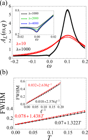
Figure 9: Finite-temperature spectral function with forward-scattering disorder plotted using the exact (solid line) and the asymptotic (dashed line) Green functions. (a) Spectral function at low ($\lambda=1000$) and high ($\lambda=10$) temperatures. Inset: asymptotic spectral function for $\lambda=1000,2000,4000$ and the exact spectral function for $\lambda=1000$. (b) Quasiparticle peak width as a function of temperature $T$ and $\xi^{-1}$ (inset). In the above, the interaction parameter $\gamma=0.1$ and $vq=-0.1$. The frequency and the length are in units of $v\alpha^{-1}$ and $\alpha$ respectively.

In the low-temperature limit, the convolution expression (32) for the spectral function at a finite temperature and disorder, can be simplified by using the Stirling formula for the single-particle Green function. We thereby obtain the following asymptotic form

$$G^{\text{ret}}_{L}(\omega,q)\sim -i\left(\frac{\alpha}{2v}\right)^{2\gamma}\frac{\Gamma\left(1-\gamma\right)}{\Gamma\left(1+\gamma\right)}\left[-i(\omega+vq)+2\pi\gamma T\right]^{\gamma-1}$$

$$\times\left[-i(\omega-vq)+2\pi(\gamma+1)T\right]^{\gamma},$$ (35)

that allows us to carry out the convolution in Eq. (32) and obtain the asymptotic expression for the disorder-averaged low-temperature Green function (see Appendix E). By choosing a complex contour on the upper complex plane, the disordered Green function is given by

$$G^{\text{ret}}_{\text{dis},L}(\omega,q)\sim G^{\text{ret}}_{L}(\omega,q+i\xi^{-1})+G^{\text{ret}}_{2,L}(\omega,q),$$ (36)

where the first term on the right hand side is the residue from the Lorentzian function and the second term comes from the integral around the branch cut, evaluated in Appendix E with the result given in Eq. (E). From this asymptotic expression, we expect the quasiparticle peak to be located at $\omega=-vq$ with an exponent $\gamma-1$ broadened by thermal and disorder effects to a width $\approx 2\pi\gamma T+v\xi^{-1}$. The zero bias anomaly at $\omega=0$ has exponent $2\gamma$ and is rounded only by the thermal effects with a scale $2\pi(2\gamma+1)T$. As shown in Fig. 9, the asymptotic formula gives a good approximation to the exact spectral function, especially at low temperature where Stirling formula approximation is valid. At zero temperature, this asymptotic prediction becomes exact as Eq. (III.3.3) is exact under such condition. However, this analytical expression only asymptotically captures the low temperature behavior of the zero-bias anomaly [inset of Fig. 9(a)]. Nevertheless, the quasiparticle peak is well described by the asymptotic formula, showing a peak width $\approx 2\pi\gamma T+v\xi^{-1}$ in Fig. 9(b).

As we have seen above, the spectral function of a single helical edge reveals the fractionalized properties of the hLL. However, (except for absence of Anderson localization due to the forbidden disorder elastic backscattering) it fails to distinguish the helical edge of a TI from a conventional LL as for example describing a spin-polarized one-dimensional conductor.

To bring out special properties of the hLL, we thus next turn to the analysis of the momentum and energy resolved inter-helical-edge tunneling, developing the theory of MRTS.

IV Two edges: Momentum-resolved tunneling

We study the momentum and energy resolved interedge tunneling spectroscopy, which, as we will show exhibits distinctive signatures of the hLL, characterizing an edge of a time-reversal invariant topological insulator with $K>3/8$ Wu et al. (2006); Xu and Moore (2006); Chou et al. (2018). A schematic of a vertical (co-planar) geometry of an experimental setup that we study is illustrated in Fig. 10 (Fig. 16). This is the TI edge counter-part of the setup studied for a conventional LL in Carpentier et al. (2002) and demonstrated experimentally Auslaender et al. (2002); Steinberg et al. (2008); Jompol et al. (2009); Tsyplyatyev et al. (2015, 2016); Jin et al. (2019). In such a setup, the momentum transfer $Q=2\pi Bd/\phi_{0}$ and frequency $\omega=eV/\hbar$ can be independently tuned by a transverse magnetic field $B$ and interedge source-drain bias $V$. In the above, $d$ denotes the distance between two edges, $\phi_{0}=h/e$ is the magnetic flux quantum and $e>0$ is the elementary charge.

In the rest of the section, we first derive the tunneling current from linear response theory. Then, bosonization is employed to anticipate both the intraedge and the interedge interactions. We discuss various situations ranging from the quantum spin Hall limit ($S_{z}$ spin conservation) to the generic situations (i.e., Rashba spin orbit coupling, disorder, distinct edge velocities and interaction strengths). The analytical expressions for the finite-temperature tunneling currents (with the same edge velocity) are the main new results of this work.

IV.1 Tunneling current

Following Ref. Carpentier et al. (2002), we consider two parallel quantum edges with a separation that allows weak interedge tunneling current. The coupled edges Hamiltonian is given by $H=H_{1}+H_{2}+H_{\text{int}}+H_{\text{tun}}$, where

$$H_{a}= \sum_{\alpha=\pm}\int\limits_{k}\left[\varepsilon_{a\alpha}(k)-\mu_{a}\right]c^{\dagger}_{a\alpha}(k)c_{a\alpha}(k),$$ (37)

$$H_{\text{int}}= U_{12}\int\limits_{x}\rho_{1}(x)\rho_{2}(x)+\sum_{a=1,2}U_{a}\int\limits_{x}\rho_{a}(x)\rho_{a}(x),$$ (38)

$$H_{\text{tun}}= -t_{0}\sum_{s=\uparrow\downarrow}\int\limits_{x}\left[c^{\dagger}_{1s}(x)c_{2s}(x)+c^{\dagger}_{2s}(x)c_{1s}(x)\right].$$ (39)

In the above expressions, $\varepsilon_{a\alpha}(k)=\epsilon_{a\alpha}(k)-\epsilon_{a\alpha}(k_{F,a\alpha})$ with $\epsilon_{a\alpha}(k)$ the band dispersion for edge $a=1,2$, $U_{a}>0$ ($U_{12}>0$) is the intraedge (interedge) Coulomb interaction (screened by a gate), $\rho_{1}$ ($\rho_{2}$) is the density of edge 1 (edge 2), $t_{0}$ is the interedge tunneling amplitude, $c_{a\alpha}$ is the annihilation operator for the chiral fermion with chirality $\alpha=+/-$ (not to be confused with the ultraviolate length scale) on the edge $a$, and $c_{as}$ is the annihilation operator for the physical fermion with spin $s$ on the edge $a$. We will consider the electrochemical potentials $\mu_{1}=eV$ ($e>0$) and $\mu_{2}=0$ such that current flows from edge 1 to 2 (2 to 1) for positive (negative) interedge source-drain bias $V$. Importantly, $c_{a\alpha}(k)$ and $c_{as}(k)$ are related to each other via Eqs. (7) and (III.1), detailed in Appendix A.

In the presence of an external magnetic field applied transversely to the plane defined by the two edges, tunneling electrons experience a Lorentz force, included through the Peierls substitution $c^{{\dagger}}_{2}c_{1}\to c^{{\dagger}}_{2}c_{1}e^{i(-e/\hbar)\int^{d}_{0}dyA_{y}(x,y)}$, where $d$ is the interedge $y$ separation. For magnetic field $\vec{B}=-B\hat{z}$, we choose the Landau gauge $\vec{A}=-Bx\hat{y}$ in which the associated Berry phase is included via the replacement $c_{1}(x)\to c_{1}(x)e^{iQx}$, where $Q=2\pi Bd/\phi_{0}$. As a result, $H_{1}$, $H_{2}$, $H_{\text{int}}$ remain unchanged and the tunneling operator, $H_{\text{tun}}$ is replaced by

$$H^{Q}_{\text{tun}}= -t_{0}\sum_{s=\uparrow\downarrow}\int\limits_{x}\left[c^{\dagger}_{1s}(x)c_{2s}(x)e^{-iQx}+\text{H.c.}\right],$$ (40)

where H.c. denotes the Hermitian conjugate.

We are interested in the tunneling current from edge 1 to edge 2. This can be derived by computing the time derivative of the charge in edge 1, $\hat{I}_{\text{tun}}=-\frac{1}{i}\left[eN_{1},H\right]=\int dx\hat{J}(x)$, where

$$\hat{J}(x)=iet_{0}\sum_{s}\left[c^{\dagger}_{2s}(x)c_{1s}(x)e^{iQx}-c^{\dagger}_{1s}(x)c_{2s}(x)e^{-iQx}\right]$$ (41)

is the tunneling current density. For the clean case, the expectation value of the tunneling current density is position independent, and thus the tunneling current $I_{\text{tun}}$ is proportional to the length of the tunneling region. For disordered case that we treat below, we will study disordered averaged current that is again $x$-independent.

To compute the expectation value of the tunneling current density, we work in interaction representation with respect to perturbation $H^{Q}_{\text{tun}}$. We select $H_{12}=H_{1}+H_{2}+H_{\text{int}}$ and $H_{I}=H^{Q}_{\text{tun}}$. The expectation value of the tunneling current density at time $t$ is given by

$$J=\frac{1}{Z}\text{Tr}\left[e^{-\beta H_{12}}\hat{U}^{\dagger}(t)\hat{J}(x)\hat{U}(t)\right],$$ (42)

where $\hat{U}(t)=\hat{U}_{12}(t)\hat{U}_{I}(t)$, $\hat{U}_{12}(t)=e^{-iH_{12}t}$, $\hat{U}_{I}(t)=\hat{T}\exp\left[-i\int_{-\infty}^{t}dt^{\prime}H^{I}_{\text{tun}}(t^{\prime})\right]$ ($\hat{T}$ the time-ordering operator), $H^{I}_{\text{tun}}(t)\equiv e^{iH_{12}t}H^{Q}_{\text{tun}}e^{-iH_{12}t}$, and $\beta$ is the inverse temperature. Importantly, $Z\equiv\text{Tr}[e^{-\beta H_{12}}]$ is the “unperturbed” partition function, with two edges in thermal equilibrium at the same temperature (due to interedge interaction), but kept at the electrochemical potential difference $\mu_{1}-\mu_{2}=eV$. Equation (42) gives the expectation of the tunneling current density at time $t$ corresponding to turning on the single-particle tunneling in the infinite past. The tunneling current $J$ is in the steady state, i.e., $t$ (and $x$) independent, and clearly vanishes to $O(t_{0})$. Relegating the details to Appendix F, standard analysis perturbative in $t_{0}$ to leading $O(t_{0}^{2})$ order gives,

$$J(\omega=eV/\hbar,Q)\approx et_{0}^{2}\left[J_{1\to 2}(\omega,Q)-J_{2\to 1}(\omega,Q)\right],$$ (43)

where

$$J_{1\to 2}(\omega,Q)= \sum_{s,s^{\prime}}\int_{-\infty}^{\infty}\!\!dt^{\prime}\int_{-\infty}^{\infty}\!\!dx^{\prime}\,e^{i\omega t^{\prime}}e^{-iQx^{\prime}}$$

$$\times\left\langle c^{\dagger}_{1s^{\prime}}c_{2s^{\prime}}(t^{\prime},x^{\prime})c^{\dagger}_{2s}c_{1s}(0,0)\right\rangle,$$ (44)

$$J_{2\to 1}(\omega,Q)= \sum_{s,s^{\prime}}\int_{-\infty}^{\infty}\!\!dt^{\prime}\int_{-\infty}^{\infty}\!\!dx^{\prime}\,e^{i\omega t^{\prime}}e^{-iQx^{\prime}}$$

$$\times\left\langle c^{\dagger}_{2s}c_{1s}(0,0)c^{\dagger}_{1s^{\prime}}c_{2s^{\prime}}(t^{\prime},x^{\prime})\right\rangle.$$ (45)

We calculate the tunneling current (42) using bosonization and utilizing imaginary time and Matsubara analytic continuation (see Appendix G). To this end, using spectral decomposition, we relate physical current $J$ to the Matsubara correlator $\mathcal{J}(i\omega_{n},Q)$,

$$J=2et_{0}^{2}\text{Im}\left[\mathcal{J}(i\omega_{n}\to\omega+i\eta,Q)\right],$$ (46)

where $\mathcal{J}(i\omega_{n},Q)$ is a Fourier transform of the imaginary-time ordered correlator defined by

$$\mathcal{J}(i\omega_{n},Q)= \int_{0}^{\beta}d\tau\int_{-\infty}^{\infty}dxe^{i(\omega_{n}\tau-Qx)}\mathcal{J}(\tau,x),$$ (47)

with the space-imaginary time correlation function given by

$$\mathcal{J}(\tau,x)= \sum_{s,s^{\prime}=\uparrow\downarrow}\left\langle\hat{T}_{\tau}c_{1s^{\prime}}^{{\dagger}}c_{2s^{\prime}}(\tau,x)c_{2s}^{{\dagger}}c_{1s}(0,0)\right\rangle.$$ (48)

IV.2 Bosonization

As we have done in Sec. III.2 for the single-edge, here too we utilize standard bosonization to treat Luttinger interaction and disorder to compute the interedge tunneling current. The imaginary-time action of the two-edge setup (without interedge tunneling) is given by $\mathcal{S}=\mathcal{S}_{12}+\mathcal{S}_{\text{dis}}$, where

$$S_{12}= \sum_{a=1,2}\,\int\limits_{\tau,x}\left\{\frac{v_{a}}{2\pi}\left[K_{a}(\partial_{x}\phi_{a})^{2}+\frac{1}{K_{a}}(\partial_{x}\theta_{a})^{2}\right]\right.$$

$$+\left.\frac{i}{\pi}\left(\partial_{x}\theta_{a}\right)\left(\partial_{\tau}\phi_{a}\right)\right\}+\frac{U_{12}}{\pi^{2}}\int\limits_{\tau,x}\left[\partial_{x}\theta_{1}(x)\right]\left[\partial_{x}\theta_{2}(x)\right]$$

$$\mathcal{S}_{\text{dis}}= \int\limits_{\tau,x}\left[V_{1}(x)\frac{1}{\pi}\partial_{x}\theta_{1}+V_{2}(x)\frac{1}{\pi}\partial_{x}\theta_{2}\right],$$ (49)

Because they appear on distinct edges, we take the disorder potentials $V_{a}(x)$ to be independent, zero-mean Gaussian fields with $\overline{V_{a}(x)V_{a^{\prime}}(y)}=\Delta_{a}\delta_{aa^{\prime}}\delta(x-y)$. We ignore interedge backscattering interactions that are only relevant under certain commensurate conditions Chou (2019). The bosonized action $S_{12}$ (IV.2) is quadratic and therefore can be written in diagonalized form. We provide the details of the explicit transformation in Appendix H analogous to Ref. Orignac et al. (2011). After diagonalizing $S_{12}$, the forward-scattering disorder, $S_{\text{dis}}$ can be taken into account via a linear transformation on the $\theta_{a}$ fields. For instance, in the limit $U_{12}=0$, where the action $S_{12}$ is in its diagonalized form, the disorder-averaged correlation function is given by

$$\overline{\left\langle e^{-in_{1}\theta_{1}(\tau,x)}e^{in_{2}\theta_{2}(\tau,x)}e^{-in_{2}\theta_{2}(0,0)}e^{in_{1}\theta_{1}(0,0)}\right\rangle}$$

$$= e^{-\sum_{a}\frac{n_{a}^{2}K_{a}^{2}\Delta_{a}}{2v_{a}^{2}}|x|}$$

$$\times\left\langle e^{-in_{1}\tilde{\theta}_{1}(\tau,x)}e^{in_{2}\tilde{\theta}_{2}(\tau,x)}e^{-in_{2}\tilde{\theta}_{2}(0,0)}e^{in_{1}\tilde{\theta}_{1}(0,0)}\right\rangle.$$ (50)

We note that this is a generalized version of Eq. (25). For $U_{12}\neq 0$, one has to first diagonalize the two-edge problem (see Appendix H), and then average over disorder to obtain the disorder-averaged correlation function.

IV.3 $S_{z}$-conserved edge: quantum spin Hall limit

For a 2D TI with an out-of-plane reflection symmetry ($z\to-z$), the spin quantization axis of the helical edge is generally along this $z$-axis due to spin-orbit coupling of the form $(\vec{p}\times\vec{E})\cdot\vec{\sigma}$, where electrons with in-plane momentum $\vec{p}$ feels an out-of-plane ($z$-axis directed) effective magnetic field due to the in-plane electric field (or crystal field polarization) $\vec{E}$, by symmetry transverse to the TI edge. Such $S_{z}$-conserved topological insulator features quantized spin-Hall conductance. It is important to note that $S_{z}$ conservation is not robust as RSOC generically breaks any spin conservation. However, it is helpful to first consider this technically simpler special case. More generic non-spin-conserving case can be built from the results derived in this section.

We first consider idealized case of $S_{z}$-conserved edges in the absence of disorder or Zeeman field. At low source-drain bias, we decompose the fermion fields so that the imaginary-time tunneling current correlator in Eq. (48) is written in terms of tunneling processes between different Fermi points

$$\mathcal{J}(\tau,x)=t^{RR}\mathcal{J}_{RR}+t^{LL}\mathcal{J}_{LL}+t^{RL}\mathcal{J}_{RL}+t^{LR}\mathcal{J}_{LR},$$ (51)

where $t^{RR}$, $t^{LL}$, $t^{RL}$, $t^{LR}$ are constants proportional to the square of the tunneling matrix elements and

$$\mathcal{J}_{RR}(\tau,x)=e^{-i\delta k_{F}x}\left\langle\hat{T}_{\tau}R_{1}^{{\dagger}}R_{2}(\tau,x)R_{2}^{{\dagger}}R_{1}(0,0)\right\rangle,$$

$$\mathcal{J}_{LL}(\tau,x)=e^{i\delta k_{F}x}\left\langle\hat{T}_{\tau}L_{1}^{{\dagger}}L_{2}(\tau,x)L_{2}^{{\dagger}}L_{1}(0,0)\right\rangle,$$

$$\mathcal{J}_{RL}(\tau,x)=e^{-ik_{F,T}x}\left\langle\hat{T}_{\tau}R_{1}^{{\dagger}}L_{2}(\tau,x)L_{2}^{{\dagger}}R_{1}(0,0)\right\rangle,$$

$$\mathcal{J}_{LR}(\tau,x)=e^{ik_{F,T}x}\left\langle\hat{T}_{\tau}L_{1}^{{\dagger}}R_{2}(\tau,x)R_{2}^{{\dagger}}L_{1}(0,0)\right\rangle.$$ (52)

In the above, $\delta k_{F}=k_{F,1}-k_{F,2}$ and $k_{F,T}=k_{F,1}+k_{F,2}$ ($k_{F,a}=k_{F,a\pm}$ as we assume TR symmetry holds on each edge). The physical tunneling current $J$ can then be obtained via the standard analytic continuation (46).

IV.3.1 Vertical geometry

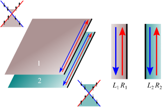
Figure 10: Vertical setup of two topological insulators in the quantum spin Hall limit. In both edges, right movers carry up spin and left movers carry down spins. The tunneling matrix elements between the two edge forbid any mixing of $L^{\dagger}_{2}R_{1}$ or $R^{\dagger}_{2}L_{1}$ (i.e. $t^{RL}=t^{LR}=0$). The tunneling current is govern by the momentum transfer of order $|k_{F,1}-k_{F,2}|$.

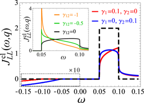
Figure 11: Zero-temperature clean (disorder-free) tunneling current with different velocities for a set of interaction parameters. The edge velocities and momentum (magnetic field) are set to $v_{1}q=-0.1$ and $v_{2}q=-0.05$. $et_{0}^{2}=1$. The black dashed line indicates the non-interacting case ($\gamma_{1}=\gamma_{2}=0$). The red (blue) curve denotes the case of interacting edge 1 (edge 2), where finite current appears for $\omega<v_{1}q$ ($\omega<v_{2}q$) due to fractionalization in chiral degrees of freedom. The inset shows the effects of repulsive interedge interaction. The interaction parameters and edge velocities are set to $\gamma_{+}=\gamma_{-}=0.05$, $v_{+}q=-0.1$ and $v_{-}q=-0.05$. The frequency and the length are in units of $v_{1}\alpha^{-1}$ and $\alpha$ respectively.

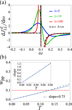
Figure 12: Finite-temperature clean (disorder-free) differential tunneling conductance for identical edge velocities with $vq=-0.1$. (a) At zero temperature, a positive delta function (negative power-law singularity) is located at $\omega=-vq\pm 0^{+}$. At finite temperatures, the two peaks are broadened and move towards the left and the right respectively. The intraedge interaction parameter is set to $2\gamma=\gamma_{1}+\gamma_{2}=0.1$. (b) Peak-to-peak distance ($w_{pp}$) as a function of $T$ and $\gamma$. The linear dependence on $T$ and $\gamma$ shows $w_{pp}\approx 7.5\gamma T$ for $w_{pp}<|vq|$ (red dashed line). The frequency and the length are in units of $v\alpha^{-1}$ and $\alpha$ respectively.

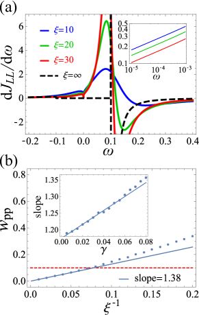
Figure 13: Zero-temperature differential tunneling conductance with forward-scattering disorders for identical edge velocities. The momentum is taken to be $vq=-0.1$. (a) Zero bias anomaly appears at $\omega=0$ for all disorder strengths $\xi^{-1}$, with the same exponent $4\gamma$ (inset), where $\xi^{-1}=\frac{K_{1}^{2}\Delta_{1}}{2v_{1}}+\frac{K_{2}^{2}\Delta_{2}}{2v_{2}}$. The interaction parameter $\gamma=0.05$. (b) Peak-to-peak distance ($w_{pp}$) as a function of $\xi^{-1}$ and $\gamma$. $w_{pp}$ is proportional to $\xi^{-1}$ for $w_{pp}<|vq|$ (red dashed line). The disorder-strength dependence becomes more sensitive for stronger interaction (inset). The frequency and the length are in units of $v\alpha^{-1}$ and $\alpha$ respectively.

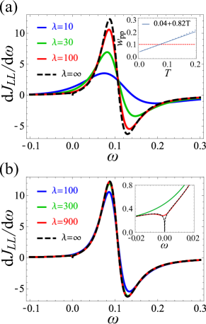
Figure 14: Finite-temperature differential tunneling conductance with forward-scattering disorders for identical edge velocities. (a) High temperature regime $\lambda\ll\xi$. Inset: the peak-to-peak distance $w_{pp}$ depends linearly on T for $w_{pp}<|vq|$ (red dashed line). (b) Low temperature regime $\lambda\gg\xi$. The momentum is taken to be $vq=-0.1$. The intraedge interaction parameter is set to $\gamma=0.05$ and disorder length $\xi=20$. The frequency and the length are in units of $v\alpha^{-1}$ and $\alpha$ respectively.

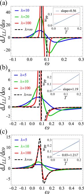
Figure 15: Differential tunneling conductance for distinct edge velocities. The edge velocities and momentum are set to $v_{+}q=-0.1$ and $v_{-}q=-0.08$. (a) Thermal broadening of the non-interacting clean tunneling peak (b) Thermal broadening of the interacting ($\gamma_{+}=0.1$, $\gamma_{-}=0$, $\gamma_{12}=0$) clean tunneling peak (c) Thermal broadening of the interacting ($\gamma_{+}=0.1$, $\gamma_{-}=0$, $\gamma_{12}=0$) tunneling peak in the presence of forward- scattering disorders $\xi=30$. The frequency and the length are in units of $v_{1}\alpha^{-1}$ and $\alpha$ respectively.

For vertical geometry illustrated in Fig. 10, two $S_{z}$ conserved edges have exactly the same spin orientation. The low-energy expressions of the fermionic $S_{z}$ eigenstate fields (Appendix A with $k_{0}\to\infty$) are given by

$$c_{a\uparrow}\approx e^{ik_{F,a}x}R_{a}(x),\quad\,c_{a\downarrow}\approx e^{-ik_{F,a}x}L_{a}(x).$$ (53)

Plugging the expression above into the imaginary-time correlator in Eq. (48), we obtain

$$\mathcal{J}_{\text{QSH},\perp}(\tau,x)=\mathcal{J}_{RR}(\tau,x)+\mathcal{J}_{LL}(\tau,x).$$ (54)

Thus, indeed, there is no tunneling current contributions corresponding to backscattering between the right and left Fermi points ($t^{RL}=t^{LR}=0$). These are forbidden by the $S_{z}$ conserving $U(1)$ spin-rotational symmetry, as such contribution requires a spin flip $\uparrow\leftrightarrow\downarrow$, whose matrix element identically vanishes in the presence of TR symmetry and in the absence of Rashba spin-orbit interaction. The momentum-resolved tunneling current is given by

$$J(\omega,Q)\approx J_{RR}(\omega,Q+\delta k_{F})+J_{LL}(\omega,Q-\delta k_{F}).$$ (55)

Below we will focus on $J_{LL}(V,Q)$ because the other term can be obtained via the relation $J_{RR}(\omega,q)=J_{LL}(\omega,-q)$ if we assume TR symmetry holds independently on each edge.

The space imaginary-time correlator can be calculated for generic intraedge LL interactions (see Appendix H), given by

$$\left\langle\hat{T}_{\tau}L_{1}^{{\dagger}}L_{2}(\tau,x)L_{2}^{{\dagger}}L_{1}(0,0)\right\rangle=-\frac{1}{(2\pi\alpha)^{2}}\prod_{b=\pm}$$

$$\times\frac{(\frac{\pi\alpha}{\beta v_{b}})^{2\gamma_{b}+1}}{\left[\sinh\left(\frac{\pi(x+iv_{b}\tau)}{\beta v_{b}}\right)\right]^{\gamma_{b}-\frac{b}{2}\gamma_{12}}\left[\sinh\left(\frac{\pi(x-iv_{b}\tau)}{\beta v_{b}}\right)\right]^{\gamma_{b}+\frac{b}{2}\gamma_{12}+1}},$$ (56)

where $v_{\pm}$ encodes the velocity in the diagonal basis, and $\gamma_{\pm}$, $\gamma_{12}$ are the anomalous exponents. The explicit forms of $v_{\pm}$, $\gamma_{\pm}$, and $\gamma_{12}$ are given in Appendix H. Notice that $\gamma_{12}<0$ ($\gamma_{12}>0$) for repulsive (attractive) interedge interaction. In particular, for $U_{12}=0$, $\mathcal{J}_{LL}$ simply reduces to a product of two single-particle Green functions with the parameters given by $\gamma_{12}=0$, $\gamma_{\pm}=\gamma_{1,2}$ and $v_{\pm}=v_{1,2}$. For identical edges ($v_{1}=v_{2}$ and $K_{1}=K_{2}$), $v_{+}$ ($v_{-}$) is associated with the velocity of symmetric (antisymmetric) interedge degrees of freedom.

In evaluating $J_{LL}(\omega,q)$, we use two different ways (detailed in Appendix F): (i) evaluate the tunneling current as a convolution of two spectral functions if $U_{12}=0$, and (ii) Analytically continue to real time and Fourier transform. In particular, method (i) works well if we assume one of the edges is non-interacting and therefore the corresponding spectral function is just a delta function. On the other hand, method (ii) works well at $T=0$ since one integral variable can be integrated over analytically in that situation.

Zero-temperature, clean case:

We start with the simplest case: zero temperature, no disorder and no interaction. In this case, the tunneling current is simply given by a box function

$$J^{0}_{LL}(\omega,q)=\frac{et_{0}^{2}\operatorname{sgn}(\omega)}{|v_{1}-v_{2}|}\Theta\left[-(\omega+v_{2}q)(\omega+v_{1}q)\right].$$ (57)

In the limit $v_{1}\to v_{2}\equiv v$, the tunneling current becomes a delta function $J^{0}_{LL}(\omega,q)=-et_{0}^{2}q\delta(\omega+vq)$. Similar to the spectral function, the presence of interaction makes the tunneling peak less sharp and display power-law features as illustrated in Fig. 11 ($et_{0}^{2}=1$ hereafter). In the presence of interedge interaction, the eigenmodes are anti-symmetric-like (subscript $-$) and symmetric-like (subscript $+$) linear combinations of the two edges. As illustrated in the inset of Fig. 11, strong repulsive interedge interaction ($U_{12}\gg v_{1}-v_{2}$) makes the tunneling current diverge at $\omega=-v_{-}q$.

Finite-temperature, clean case:

Now, we discuss the finite-temperature tunneling current in the absent of disorder. For the special case $v_{1}=v_{2}$ and $U_{12}=0$, we can perform Fourier transform analytically [using Eq. (D)]. The finite-temperature clean tunneling current is given by

$$J^{\text{cl}}_{LL}(\omega,q) =-2et_{0}^{2}\left(\frac{2\pi\alpha}{\beta v}\right)^{4\gamma}\frac{1}{4\pi^{2}v}\sin(2\pi\gamma)$$

$$\quad\,\times\text{Im}\left\{B\left[\frac{\beta(-i\omega+ivq)}{4\pi}+\gamma+1,-1-2\gamma\right]\right.$$

$$\quad\quad\,\,\times\left.B\left[\frac{\beta(-i\omega-ivq)}{4\pi}+\gamma,1-2\gamma\right]\right\},$$ (58)

where $\gamma=(\gamma_{1}+\gamma_{2})/2$ is the average interaction parameter. In the noninteracting limit (i.e., $\gamma=0$ and $U_{12}=0$), the tunneling current becomes temperature independent as the strict kinematic constraint of two equal velocity, in contrast to the distinct velocity case discussed below. For identical edges ($K_{1}=K_{2}=K$ and $v_{1}=v_{2}=v$), we can also obtain analytical expression for $U_{12}\neq 0$ because the space-time correlator in Eq. (56) only depends on the velocity of anti-symmetric mode $v_{-}$. The resulting clean tunneling current takes the same form as Eq. (58) but with the replacement $v\to v_{-}=v\sqrt{1-U_{12}K/2\pi^{2}v}$ and $\gamma\to(K_{-}+K_{-}^{-1})/4-1/2$, where $K_{-}=K/\sqrt{1-U_{12}K/2\pi^{2}v}$. At zero temperature, the tunneling current exhibits a power singularity at $\omega=-vq$, which becomes two peaks (or one anti-symmetric peak) for the differential tunneling conductance as shown in Fig. 12. Remarkably, the peak-to-peak distance is captured by $w_{pp}\approx 7.5\gamma T$ for $w_{pp}<|vq|$. For $w_{pp}>|vq|$, the broadening of the left (positive-valued) peak is dominated by the thermal excitation around the Fermi point and the linear dependence breaks down.

Disordered case:

Now we discuss the effects of forward-scattering disorder (evaluated through a convolution with a Lorentzian characterized by a disorder strength $\xi^{-1}=\frac{K_{1}^{2}\Delta_{1}}{2v_{1}}+\frac{K_{2}^{2}\Delta_{2}}{2v_{2}}$). At zero temperature, exact analytical expression is derived in Eq. (151). Similar to spectral function in a single edge, the differential tunneling conductance features a disorder-induced ZBA in a power-law form $dJ_{LL}/d\omega\propto|\omega|^{4\gamma}$, independent of disorder strength, as shown in Fig. 13(a). The peak-to-peak distance exhibits a linear dependence on $\xi^{-1}$ for $w_{pp}<|vq|$ as illustrated in Fig. 13(b). Different from thermal broadening, the disorder can smear out the peak even at zero temperature (see the inset). For $w_{pp}>|vq|$, tunneling weights from opposite momentum (i.e. having different sign of q) will start to contribute, which gives opposite currents, and the linear dependence fails. At finite temperature, $w_{pp}$ still depends linearly on $T$ despite the presence of finite disorder [see Fig. 14(a)], which suggests that the disorder strength $\xi^{-1}$ and interaction strength $\gamma$ can both be quantified through a temperature dependence measure on $w_{pp}$. Figure 14(b) shows that ZBA gets rounded at finite temperature. The thermal rounding takes the similar form as Eq. (34).

Distinct velocity:

When $U_{12}>0$, the system is in general characterized by two distinct velocities $v_{\pm}$ with $v_{-}<v_{+}$ (even for identical edges) and an exponent $\gamma_{12}$ [given by Eq. (134)], encoding the correction due to the interaction between the two edges ($U_{12}$). The interaction-driven inequality of velocities, $v_{-}<v_{+}$ has qualitatively important effects on the tunneling current. This is in contrast to nonvanishing $\gamma_{12}$, that does not modify the tunneling current qualitatively. We therefore take $\gamma_{12}=0$ for simplicity. With such an approximate, the effects of interedge interaction $U_{12}$ still enter by modifying $v_{\pm}$ and $\gamma_{\pm}$. The $\gamma_{12}=0$ approximation affects the analytical form of the tunneling peak in the clean limit (see the inset of Fig. 11) but does not change the thermal broadening rate because the exponential decay factor at large time does not depend on $\gamma_{12}$ [see Eq. (56)]. Also, in the presence of the disorders, by power counting in Eq. (56) we expect that the ZBA of the differential tunneling conductance to be characterized by a power-law exponent $2\gamma_{+}+2\gamma_{-}$, which is also independent of $\gamma_{12}$ (but does dependent on $U_{12}$). At zero temperature, the clean differential tunneling conductance is featured by two singularities located at $\omega=-v_{+}q$ and $\omega=-v_{-}q$. One prominent effect of $v_{+}\neq v_{-}$, as illustrated in Fig. 15(a), is on thermal broadening of the tunneling peak, even in the non-interacting limit. The absence of thermal broadening in the same velocity case is due to the strict kinematic constraint which is fine-tuned. Remarkably, the thermal broadening (due to distinct velocities) is linear in $T$ at high temperature [see inset of Fig. 15(a)]. The temperature dependence should also be proportional to the velocity difference, i.e. $\propto(v_{+}-v_{-})T$, if $v_{+}-v_{-}\ll v_{+}+v_{-}$. In the presence of interaction, with or without disorders, the peak-to-peak distance still exhibits a considerable linear in $T$ regime [see Fig. 15(b) and (c)]. However, the zero temperature peak width (or $w_{pp}$) is now determined by both the disorder strength $\xi^{-1}$ and $(v_{+}-v_{-})q$. In evaluating Fig. 15(b) and (c), we set one of the interaction parameter to zero $\gamma_{-}=0$ and use the asymptotic expression in Eq. (36) for the symmetric-like branch for computational convenience. More generally, we expect the interaction facilitated thermal broadening rate is determined by $\gamma_{+}+\gamma_{-}$.

IV.3.2 Horizontal geometry

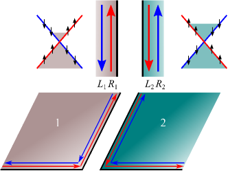
Figure 16: Horizontal setup of two topological insulators in the quantum spin Hall limit. The two co-moving edges have opposite spin orientations. As a result, the tunneling matrix element forbids the mixing of $R^{\dagger}_{2}R_{1}$ and $L^{\dagger}_{2}L_{1}$ (i.e. $t^{RR}=t^{LL}=0$). The tunneling current is govern by the momentum transfer of order $|k_{F,1}+k_{F,2}|$.

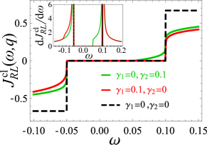
Figure 17: Zero-temperature clean (disorder-free) tunneling current for a set of intraedge interaction parameters. The interedge interaction is ignored in this plot. The edge velocities and momentum are set to $v_{1}q=-0.1$ and $v_{2}q=-0.05$. The black dashed line indicates the non-interacting case ($\gamma_{1}=\gamma_{2}=0$). The red (green) line denotes the case that edge 1 (edge 2) becomes interacting, where finite current appears for $\omega<v_{1}q$ ($\omega>-v_{2}q$) due to fractionalization in chiral degrees of freedom. The inset shows the corresponding differential tunneling conductance. The frequency and the length are in units of $v_{1}\alpha^{-1}$ and $\alpha$ respectively.

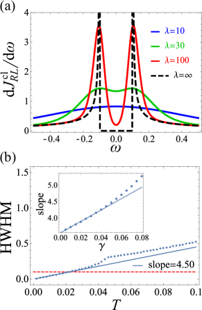
Figure 18: Finite-temperature clean (disorder-free) differential tunneling conductance for identical edge velocities with $vq=-0.1$. (a) At zero temperature, two power-law singularities are located at $\omega=\pm vq$. At finite temperature, the two peaks get broadened and merge into a single peak at $\omega=0$ with increasing temperature. The intraedge interaction parameter is set to $2\gamma=\gamma_{1}+\gamma_{2}=0.1$. (b) Half width at half maximum versus temperature. The linear dependence on $T$ holds for $\text{HWHM}<|vq|$ (red dashed line) and the slope has an $\text{offset}\approx 3.5$ in the non-interacting limit (inset). The frequency and the length are in units of $v\alpha^{-1}$ and $\alpha$ respectively.

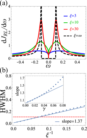
Figure 19: Zero-temperature differential tunneling conductance with forward-scattering disorders for identical edge velocities. The momentum is taken to be $vq=-0.1$. (a) Zero bias anomaly appears at $\omega=0$ for all $\xi^{-1}$, with the same exponent $4\gamma$, where $\xi^{-1}=\frac{K_{1}^{2}\Delta_{1}}{2v_{1}}+\frac{K_{2}^{2}\Delta_{2}}{2v_{2}}$ characterizing the strength of disorder. The interaction parameter $\gamma=0.05$. (b) Half width at half maximum versus temperature. HWHM is proportional to $\xi^{-1}$ for $\text{HWHM}<|vq|$ (red dashed line). Inset: The slope $\approx 1$ in the noninteracting limit and the disorder-strength dependence becomes more sensitive for stronger interaction. The frequency and the length are in units of $v\alpha^{-1}$ and $\alpha$ respectively.

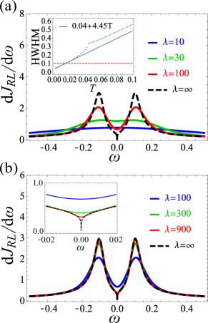
Figure 20: Finite-temperature differential tunneling conductance with forward-scattering disorders for identical edge velocities. The momentum is taken to be $vq=-0.1$. The intraedge interaction parameter is set to $\gamma=0.05$ and disorder length $\xi=30$. (a) Thermal broadening of the tunneling peak. Inset: Half width at half maximum depends linearly on T for $\text{HWHM}<|vq|$ (red dashed line) (b) Thermal rounding of zero-bias anomaly. The frequency and the length are in units of $v\alpha^{-1}$ and $\alpha$ respectively.

As a complementary experimental setup, we consider horizontal geometry illustrated in Fig. 16, where the right/left movers of the two edges have opposite spins. In this case, the low-energy expressions of the fermionic fields are given by

$$c_{1\uparrow}\approx e^{ik_{F,1}x}R_{1}(x),\quad\,c_{1\downarrow}\approx e^{-ik_{F,1}x}L_{1}(x)$$

$$c_{2\uparrow}\approx e^{-ik_{F,2}x}L_{2}(x),\quad\,c_{2\downarrow}\approx e^{ik_{F,2}x}R_{2}(x).$$ (59)

The imaginary-time correlator is now given by

$$\mathcal{J}_{\text{QSH},\parallel}(\tau,x)=\mathcal{J}_{RL}(\tau,x)+\mathcal{J}_{LR}(\tau,x),$$ (60)

where $t^{RR}=t^{LL}=0$, by $S_{z}$ conserving $U(1)$ spin rotational symmetry. The momentum-resolved tunneling current is given by

$$J(\omega,Q)\approx J_{RL}(\omega,Q+k_{F,T})+J_{LR}(\omega,Q-k_{F,T}).$$ (61)

Below we will focus on $J_{RL}(\omega,q)$ because the reverse current contribution can be obtained via the relation $J_{LR}(\omega,q)=J_{RL}(\omega,-q)$, if we assume that TR symmetry holds independently on each edge (i.e., small Zeeman field).

The space imaginary-time correlator can be calculated with both the intraedge and interedge LL interactions (see Appendix H), given by

$$\left\langle\hat{T}_{\tau}L_{1}^{{\dagger}}R_{2}(\tau,x)R_{2}^{{\dagger}}L_{1}(0,0)\right\rangle=\frac{1}{(2\pi\alpha)^{2}}\prod_{b=\pm}$$

$$\!\times\!\!\frac{(\frac{\pi\alpha}{\beta v_{b}})^{2\gamma_{b}+1}}{\left[\sinh\left(\!\frac{\pi(x+iv_{b}\tau)}{\beta v_{b}}\!\right)\right]^{\frac{1+2\gamma_{b}+b\bar{\gamma}_{12}}{2}}\left[\sinh\left(\!\frac{\pi(x-iv_{b}\tau)}{\beta v_{b}}\!\right)\right]^{\frac{1+2\gamma_{b}-b\bar{\gamma}_{12}}{2}}},$$ (62)

where $\bar{\gamma}_{12}$ are the anomalous exponents. Note that $\bar{\gamma}_{12}$ is different from $\gamma_{12}$; the explicit expression is given in Appendix H. For $U_{12}=0$, $\mathcal{J}_{RL}$ simply reduces to a product of two single-particle Green functions with the parameters given by $\bar{\gamma}_{12}=1$, $\gamma_{\pm}=\gamma_{1,2}$ and $v_{\pm}=v_{1,2}$.

Zero-temperature, clean case:

In the zero temperature, non-interacting and clean limit, the tunneling current is simply given by a step function

$$J^{0}_{RL}(\omega,q)=\frac{et_{0}^{2}\operatorname{sgn}(\omega)}{|v_{1}+v_{2}|}\Theta\left[(\omega-v_{2}q)(\omega+v_{1}q)\right].$$ (63)

As shown in Fig. 17, the presence of interaction smears out the steps and generate finite tunneling weights at opposite momentum, i.e. $\omega>-v_{2}q$ ($\omega<v_{1}q$) for $\gamma_{2}>0$ ($\gamma_{1}>0$). We also plot the differential tunneling conductance in the inset of Fig. 17.

Finite-temperature, clean case:

For the special case $v_{1}=v_{2}$ and $U_{12}=0$, we can derive the finite-temperature clean tunneling current [using Eq. (D)], given by

$$J^{\text{cl}}_{RL}(\omega,q) =-2et_{0}^{2}\left(\frac{2\pi\alpha}{\beta v}\right)^{4\gamma}\frac{1}{4\pi^{2}v}\sin(2\pi\gamma)$$

$$\quad\,\times\text{Im}\left\{B\left[\frac{\beta(-i\omega+ivq)}{4\pi}+\gamma+\frac{1}{2},-2\gamma\right]\right.$$

$$\quad\quad\,\,\times\left.B\left[\frac{\beta(-i\omega-ivq)}{4\pi}+\gamma+\frac{1}{2},-2\gamma\right]\right\}.$$ (64)

In this case, the tunneling current (differential tunneling conductance) is an odd (even) function in $\omega$. With increasing temperature, the two peaks of the differential tunneling conductance at $\omega=\pm vq$ are broadened, move toward the center and merge into a single peak at $\omega=0$ [see Fig. 18(a)]. The thermal broadening of the peaks is quantified by the half width at half maximum (HWHM). Specifically, we calculate the distance between the positions of the right peak and its right half maximum. The peak width is proportional to the temperature until the two (left and right) peaks start to merge [see Fig. 18(b)]. Although the magnitude of the two edge velocities are identical, the kinematic constraint on the tunneling current is weaker than that in the left-to-left tunneling discussed previously. As a result, there is a strong thermal broadening even in the non-interacting limit [see the inset in Fig. 18(b)].

Disordered case:

Now we discuss the effects of forward-scattering disorder. At zero temperature, the increasing strength of forward-scattering disorder smears out the power-law peak but the position of the peaks do not move much (comparing to the thermal effect) as shown in Fig. 19(a). Again, a ZBA appears with an exponent $2\gamma_{1}+2\gamma_{2}$ independent of the disorder strength. The disorder-induced peak broadening is proportional to the strength $\xi^{-1}$ for $\text{HWHM}<|vq|$. For $\text{HWHM}>|vq|$, the linear dependence on $\xi^{-1}$ still roughly holds since the two peak do not merge [see Fig. 19(b)]. At finite temperatures, there is a crossover between the zero-temperature disordered and the finite-temperature clean behaviors [see Fig. 20(a)] with the peak width increased linearly with temperature for $\text{HWHM}<|vq|$. Figure 20(b) shows that ZBA gets rounded at finite temperatures. The effect due to thermal rounding is similar to Eq. (34).

Distinct velocity:

For distinct edge velocities, the zero-temperature clean tunneling current is qualitatively modified from the case of identical velocities, as shown in Fig. 17. However, in the presence of forward-scattering disorders, the power-law peaks become rounded and a ZBA appears characterized by a modified exponent $2\gamma_{+}+2\gamma_{-}$. The linear dependence of the peak width still holds and can be used for quantifying the disorder and interaction strengths.

IV.3.3 Misaligned spin quantization axes

As discussed above, for the ideal cases where the two spin quantization axes are parallel, some of the tunneling processes vanish identically in the TR symmetric limit. However, when the two 2D TI layers are misaligned such that the quantization axes differ by an angle $\phi_{12}\in[0,\pi/2]$, all the tunneling amplitudes in Eq. (51) are expected to be nonzero. To $O(t_{0}^{2})$ order, the tunneling constants obey the sum rule

$$\sum_{\alpha^{\prime}=R,L}t^{\alpha\alpha^{\prime}}=1,$$ (65)

and the ratio $t^{RL}/t^{RR}=\tan^{2}\phi_{12}$ $(=\cot^{2}\phi_{12})$ for the vertical (co-planar) setup. Also, $t^{RR}=t^{LL}$ and $t^{RL}=t^{LR}$ due to the time-reversal symmetry on the edges, which will be broken if we consider Zeeman effect discussed in the next section.

IV.4 Other subleading corrections

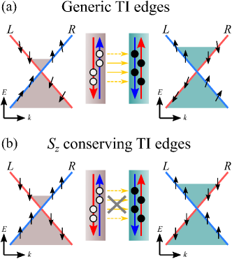
Figure 21: Bands, spin textures, and single-particle tunnelings between TI edges, illustrated with the horizontal setup in Fig. 16. (a) Generic TI edges include Rashba spin-orbit coupling, leading to the illustrated momentum-dependent spin texture. Despite a non-conservation of $S_{z}$, TR symmetry protects a degenerate pair of Kramer states at every energy. The tunnelings can be classified by small momentum transfer (yellow solid arrows) and large momentum transfer (yellow dashed arrows.) (b) $S_{z}$ conserving TI edges. Due to the additional conservation of $S_{z}$, the small momentum transfer tunneling is forbidden.

IV.4.1 Zeeman effect

With Zeeman effect, for vertical geometry $\vec{B}\perp\hat{z}$, we note there will be finite tunneling current between right and left Fermi points and a gap will open at the charge neutral point. In contrast, for the co-planar geometry $\vec{B}\parallel\hat{z}$, the spin quantization axis will remain along the z-axis in the presence of the magnetic field and tunneling current contribution between the two right/left Fermi points will remain zero. The charge neutral point in this case remains gapless but moves away from the time-reversal point in the Brillouin zone.

IV.4.2 Rashba spin-orbit coupling

The effects of Rashba spin-orbit coupling on MRTS is a bit more complicated, but as we discuss below, is sub-leading for a large bare (without RSOC) tunneling amplitude. We expect the RSOC effects to be manifest for the right-to-right (right-to-left) tunneling process for the perfectly-aligned horizontal (vertical) geometry, where bare tunneling vanishes otherwise. For concreteness, here we briefly discuss the perfectly-aligned horizontal geometry with identical edges [see Fig. 21(a)], focusing on tunneling current between two right Fermi points. The analysis for the right-to-left tunneling current and for the vertical geometry are quite similar.

Using chiral decomposition in Eqs. (78) and (79), we express the “hopping term” as follows:

$$\sum_{s=\uparrow\downarrow}c^{{\dagger}}_{1s}c_{2s}$$

$$\approx e^{-i\delta k_{F}x}\left\{\frac{\delta k_{F}k_{F,T}}{k_{0}^{2}}R^{{\dagger}}_{1}R_{2}+i\frac{k_{F,T}}{k_{0}^{2}}\partial_{x}(R^{{\dagger}}_{1}R_{2})\right.$$

$$\quad+\left.i\frac{\delta k_{F}}{k_{0}^{2}}\left[\partial_{x}(R^{{\dagger}}_{1})R_{2}-R^{{\dagger}}_{1}\partial_{x}(R_{2})\right]\right\}$$

$$\quad+\text{(hopping between other Fermi points)},$$ (66)

where $\delta k_{F}=k_{F,1}-k_{F,2}$, $k_{F,T}=k_{F,1}+k_{F,2}$. We assume that $k_{F,T}\gg\delta k_{F}$, so only the first two terms in Eq. (66) are considered. The imaginary-time correlator for the right-to-right tunneling current is given by

$$\mathcal{J}_{RR}^{\text{RSOC}}(\tau,x)= e^{-i\delta k_{F}x}\left[\alpha_{12}\left\langle\hat{T}_{\tau}R_{1}^{{\dagger}}R_{2}(\tau,x)R_{2}^{{\dagger}}R_{1}(0,0)\right\rangle\right.$$

$$+\left.\alpha_{12}^{\prime}\left\langle\hat{T}_{\tau}[\partial_{x}R_{1}^{{\dagger}}R_{2}](\tau,x)[R_{2}^{{\dagger}}R_{1}](0,0)\right\rangle\right.$$

$$-\left.\alpha_{12}^{\prime}\left\langle\hat{T}_{\tau}[R_{1}^{{\dagger}}R_{2}](\tau,x)[\partial_{x}R_{2}^{{\dagger}}R_{1}](0,0)\right\rangle\right.$$

$$+\left.\alpha_{12}^{\prime\prime}\left\langle\hat{T}_{\tau}[\partial_{x}R_{1}^{{\dagger}}R_{2}](\tau,x)[\partial_{x}R_{2}^{{\dagger}}R_{1}](0,0)\right\rangle\right]$$ (67)

where $\alpha_{12}=(\delta k_{F}k_{F,T})^{2}/k_{0}^{4}$, $\alpha_{12}^{\prime}=i\delta k_{F}k_{F,T}^{2}/k_{0}^{4}$ and $\alpha_{12}^{\prime\prime}=k_{F,T}^{2}/k_{0}^{4}$.

For distinct edges, we typically expect that $\alpha_{12}\gg\alpha_{12}^{\prime},\alpha_{12}^{\prime\prime}$, and thus the momentum-resolved tunneling current is qualitatively the same as that in the quantum spin Hall limit. However, for the identical edges considered here, the $\alpha_{12}$ term becomes less important as $\delta k_{F}\to 0$, for which additional contributions come from the derivative terms in Eq. (67) are manifest. Despite the complicated structures in the tunneling currents, we argue that there are still universal features whether RSOC is included or not. Firstly, we expect the “single-peak” (“no-peak”) feature of $J_{LL}$ ($J_{RL}$) still remains for the derivatives on the space-time correlation functions change the exponent by “-1”, which, by dimensional analysis make the tunneling current less divergent. Another observation is that the linear-$T$ thermal broadening of the tunneling peak should be robust against RSOC, since the derivatives on the space-time correlation functions does not change the exponential decay factors at large $v\tau,x$. The correlation function can in principle be calculated by bosonization, but we do not pursue this analysis here.

IV.4.3 Interedge backscattering

Besides the correction in the tunneling current matrix element, the RSOC also enables backscattering interactions Schmidt et al. (2012); Kainaris et al. (2014); Chou et al. (2015), contributing to the finite-temperature broadening. The most relevant (in renormalization group analysis) perturbations involve both edges. For strong interaction $K_{\pm}<3/4$ (identical edges), instabilities appear Chou (2019) due to interplay of interedge interactions and forward-scattering disorder, the tunneling current of the resulting phase is beyond the scope of present work, but would be of interest to study in the future in a context of specific experiments.

V Conclusion

In this manuscript, we developed a finite-temperature spectroscopy of a hLL as realized on the boundary of the 2D time-reversal symmetric TI. In our analysis we utilized standard bosonization which enabled analytical progress in the presence of interactions. Moreover, because TR symmetry forbids backscattering components of disorder, allowing only forward scattering nonmagnetic impurities, enabled us to treat disorder in a hLL exactly. We focused on the weakly interacting regime ($K>3/8$), thereby avoiding edge instability Wu et al. (2006); Xu and Moore (2006); Chou et al. (2018). We thereby analyzed in great detail various limits of finite-temperature spectral functions and the interedge tunneling currents in the momentum-resolved tunneling spectroscopy. For MRTS we explored the vertical and horizontal geometries with long edges, detailing effects of TR invariant disorder, interaction, and temperature. We studied how the product expression for the tunneling current (valid in the noninteracting limit between edges) is qualitatively modified by the interedge interaction and distinct edge velocities. Our theory thus provides a detailed characterization of the emergent hLL, complementary to the standard transport measurements.

Our analysis was limited to the hLL phase, that appears in the weakly interacting ($K>3/8$) regime of TI edges. However, as discussed in Chou et al. (2018), TI edge states can become glassy and localized due to an interplay of disorder and interaction for $K<3/8$ Wu et al. (2006); Xu and Moore (2006). This scenario might be relevant to the earlier InAs/GaSb experiments Du et al. (2015); Li et al. (2015). A detailed characterization of the finite-temperature spectroscopy in this regime is beyond present work, but in light of various experiments is of interest to explore by methods developed here. Here, we only speculate about some qualitative zero-temperature features inside this glassy edge states. The localized edges for $K<3/8$ spontaneously break time-reversal symmetry and exhibit half-charge excitations, corresponding to domain-walls or equivalently the Luther-Emory fermions. We expect that this time-reversal breaking eliminates sensitivity of the response to an applied magnetic field. We thus expect that the localized nature of the glassy edge will lead to only weakly momentum-dependent tunneling spectroscopy, contrasting to that found above for hLL. It might be challenging to distinguish the single-particle Anderson localization (i.e., trivial edge state) and the unconventional half-charge localization (i.e. TI edge with $K<3/8$). Exploring the unique spectroscopic signatures for the nontrivial half-charge localization is an interesting future direction.

We conclude by noting that momentum in MRTS setup is tuned by a magnetic field $B$ that explicitly breaks TR symmetry. Quite generally, we expect TI phase and the associated hLL edges to be stable as long as the Zeeman energy associated with this TR breaking is weak enough, to be below the bulk gap. Nevertheless, the bottleneck of our theory is set by the magnetic field induced disorder backscattering with a localization length $l_{\text{loc}}(B)$. Although, as we discussed in Sec. IV.4.1, the effect of magnetic field may vary based on the specific setup, we still expect our theory to be valid in a sufficiently weak magnetic field such that the length of hLL edge $l_{\text{edge}}\ll l_{\text{loc}}(B)$. As illustrated in Fig. 4, the momentum transfer $Q=2\pi Bd/\phi_{0}$ required to access the low-bias tunneling region between the same ($J_{RR}/J_{LL}$) and the opposite ($J_{RL}/J_{RL}$) chiral movers are given by the Fermi wavevector difference $|k_{F,1}-k_{F,2}|$ and the sum $|k_{F,1}+k_{F,2}|$ respectively. Clearly then, typical wavevector range we want to explore is set by the scale of Fermi wavevector, e.g., for $Q=|k_{F,1}-k_{F,2}|=0.01\text{ nm}^{\text{-1}}$ and tunneling distance $d=15\text{ nm}$, the corresponding magnetic flux density $B\sim 1\text{T}$. In principle, the TI materials with larger bulk gap (e.g., WTe₂ Wu et al. (2018), WSe₂ Chen et al. (2018); Ugeda et al. (2018), and BiSiC Reis et al. (2017)) are best suited for MRTS experiments due to the suppression of backscattering generated by, e.g., charge puddles Väyrynen et al. (2013) and Zeeman gap of edge bands Skolasinski et al. (2018).

Appendix A chiral decomposition of generic hLL

In the presence of the Rashba spin-orbit coupling (RSOC), the spin is no longer a good quantum number, and the single particle band develops a momentum-dependent spin texture. The orientation of the spin quantization axis at momentum $k$ relative to the one at $k=0$ (denoted by $\uparrow$ and $\downarrow$) is given as follows Schmidt et al. (2012):

$$\left[\begin{array}[]{cc}c_{k\uparrow}\\ c_{k\downarrow}\end{array}\right]=B_{k}\left[\begin{array}[]{cc}c_{k+}\\ c_{k-}\end{array}\right],$$ (72)

where (with the convention $k$ in x-direction and the normal vector of the 2D TI plane in z-direction)

$$B_{k}= e^{-i\sigma_{2}\theta_{k}}=\left[\begin{array}[]{cc}\cos(\theta_{k})&-\sin(\theta_{k})\\ \sin(\theta_{k})&\cos(\theta_{k})\end{array}\right]\approx\left[\begin{array}[]{cc}1&-\frac{k^{2}}{k_{0}^{2}}\\ \frac{k^{2}}{k_{0}^{2}}&1\end{array}\right].$$ (77)

The form of $B_{k}$, encoding the spin texture is determined by the unitarity and the time-reversal symmetry (in a particular phase convention) with spin orientation at momentum $k$ obeying $\theta_{k}=\theta_{-k}$. In the last equality in (77), we use $\theta_{k}\approx(k/k_{0})^{2}$ for small $k$, where $k_{0}$ is a parameter characterizing the scale of spin rotation across the band. To study the low-energy physics around Fermi points, we can expand $k\approx\pm k_{F}+q$ for the right (+) and left (-) movers, respectively. The field operator for spin up is then given by

$$c_{\uparrow}(x)= \int_{k}e^{ikx}c_{\uparrow}(k)$$

$$\approx e^{ik_{F}x}\int_{|q|\ll k_{F}}e^{iqx}c_{\uparrow}(k_{F}+q)$$

$$+e^{-ik_{F}x}\int_{|q|\ll k_{F}}e^{iqx}c_{\uparrow}(-k_{F}+q)$$

$$\approx e^{ik_{F}x}\int_{|q|\ll k_{F}}e^{iqx}c_{+}(k_{F}+q)$$

$$-e^{-ik_{F}x}\int_{|q|\ll k_{F}}e^{iqx}\left[\frac{k_{F}^{2}}{k_{0}^{2}}-\frac{2k_{F}q}{k_{0}^{2}}\right]c_{-}(-k_{F}+q)$$

$$= e^{ik_{F}x}\int_{|q|\ll k_{F}}e^{iqx}c_{+}(k_{F}+q)$$

$$-e^{-ik_{F}x}\left[\frac{k_{F}^{2}}{k_{0}^{2}}+i\frac{2k_{F}}{k_{0}^{2}}\partial_{x}\right]\int_{|q|\ll k_{F}}e^{iqx}c_{-}(-k_{F}+q)$$

$$= e^{ik_{F}x}R(x)-e^{-ik_{F}x}\left[\frac{k_{F}^{2}}{k_{0}^{2}}+i\frac{2k_{F}}{k_{0}^{2}}\partial_{x}\right]L(x),$$ (78)

Similarly, the field operator for spin down can be expressed as

$$c_{\downarrow}(x)= \int_{k}e^{ikx}c_{k\downarrow}$$

$$\approx e^{ik_{F}x}\left[\frac{k_{F}^{2}}{k_{0}^{2}}-i\frac{2k_{F}}{k_{0}^{2}}\partial_{x}\right]R(x)+e^{-ik_{F}x}L(x).$$ (79)

Appendix B Bosonization convention

To treat interaction and disorder nonperturbatively we utilize standard bosonization method Shankar (2017) (with the convention consistent with Refs. Chou et al. (2018); Chou (2019)), where left ($L$) and right ($R$) moving fermionic low-energy excitations can be represented through the bosonic fields $\phi_{R,L}$, according to

$$R(x)= \frac{1}{\sqrt{2\pi\alpha}}e^{i\phi_{R}(x)}=\frac{1}{\sqrt{2\pi\alpha}}e^{i\left[\phi(x)+\theta(x)\right]}$$

$$L(x)= \frac{1}{\sqrt{2\pi\alpha}}e^{i\phi_{L}(x)}=\frac{1}{\sqrt{2\pi\alpha}}e^{i\left[\phi(x)-\theta(x)\right]},$$ (80)

where $\alpha$ is the ultraviolet cutoff length scale below which the low-energy description breaks down. The “phase-like” ($\phi$) and the “phonon-like” ($\theta$) bosonic fields obey the following commutation relation

$$[\partial_{x}\theta(x),\phi(x^{\prime})]=i\pi\delta(x-x^{\prime}).$$ (81)

The commutation relations of the right and left bosons are given by

$$[\phi_{R}(x),\phi_{R}(x^{\prime})]=i\pi\operatorname{sgn}(x-x^{\prime})$$

$$[\phi_{L}(x),\phi_{L}(x^{\prime})]=-i\pi\operatorname{sgn}(x-x^{\prime})$$

$$[\phi_{R}(x),\phi_{L}(x^{\prime})]=i\pi.$$ (82)

The key characteristic of a helical Luttinger liquid (as contrasting with superficially similar, spinless fermions) is the anomalous time-reversal operation, $\mathcal{T}$, with $R\rightarrow L$, $L\rightarrow-R$, and $i\rightarrow-i$, and $\mathcal{T}^{2}=-1$, akin to spin-1/2 fermions. On the corresponding bosonic operators $\mathcal{T}$ acts according to, $\phi\rightarrow-\phi+\frac{\pi}{2}$, $\theta\rightarrow\theta-\frac{\pi}{2}$, and $i\rightarrow-i$. One of the immediate consequence of the anomalous time reversal symmetry is the absence of elastic backscattering (i.e., forbidding $L^{\dagger}R$ and $R^{\dagger}L$), that clearly breaks it. As discussed in the main text, the forward-scattering nonmagnetic disorder (allowed by $\mathcal{T}$) alone cannot result in Anderson localization, and thus TI hLL edge is stable to nonmagnetic impurities in the absence of strong interactions.

Appendix C Derivation of clean imaginary time-ordered Green function

In this appendix, we provide a step-by-step derivation of imaginary time-ordered single fermion Green function in $\tau,x$ domain at finite temperature using the bosonization formalism. The generalization to multi-particle Green function for a harmonic bosonized model is straightforward utilizing Wick’s theorem. With the helical edge Hamiltonian $H_{\text{hLL}}=H_{\text{0}}+H_{\text{int}}$ given by Eqs. (9) and (III.1), the bosonized imaginary-time action reads

$$S_{\text{hLL}}=\int\limits_{\tau,x}\left\{\frac{i}{\pi}\left(\partial_{x}\theta\right)\left(\partial_{\tau}\phi\right)+\frac{v}{2\pi}\left[K\left(\partial_{x}\phi\right)^{2}+\frac{1}{K}\left(\partial_{x}\theta\right)^{2}\right]\right\}.$$ (83)

Using the chiral decomposition $\Psi(x)=e^{ik_{F}x}R(x)+e^{-ik_{F}x}L(x)$ of fermionic field at low energy, the imaginary time-ordered single fermion correlation function is given by

$$\mathcal{G}(\tau,x)= \left\langle\Psi(\tau,x)\Psi^{{\dagger}}(0,0)\right\rangle_{\tau}$$

$$= e^{ik_{F}x}\langle R(\tau,x)R^{{\dagger}}(0,0)\rangle_{\tau}+e^{-ik_{F}x}\langle L(\tau,x)L^{{\dagger}}(0,0)\rangle_{\tau},$$ (84)

where the subscript $\tau$ denotes imaginary time-ordered average, and for forward scattering only, appropriate to the hLL studied in this manuscript, the cross term vanishes. We calculate the left mover contribution and then deduce the right mover component using the time-reversal operation according to the relation $\langle R(\tau,x)R^{{\dagger}}(0,0)\rangle_{\tau}=\langle L(\tau,x)L^{{\dagger}}(0,0)\rangle^{*}_{\tau}$. Using the bosonization representation Eq. (B) and Wick’s theorem for the Gaussian bosonic phase fields, the left-moving part is given by

$$\langle L(\tau,x)L^{{\dagger}}(0,0)\rangle_{\tau} =\frac{1}{2\pi\alpha}e^{-\frac{1}{2}\langle[\phi(\tau,x)-\theta(\tau,x)-\phi(0,0)+\theta(0,0)]^{2}\rangle_{\tau}}$$

$$=\frac{1}{2\pi\alpha}e^{-\frac{1}{2}(K+K^{-1})F_{1}(\tau,x)+F_{2}(\tau,x)},$$ (85)

where

$$F_{1}(\tau,x)= 2K[\langle\phi(0,0)\phi(0,0)\rangle_{\tau}-\langle\phi(\tau,x)\phi(0,0)\rangle_{\tau}]$$

$$= 2K^{-1}[\langle\theta(0,0)\theta(0,0)\rangle_{\tau}-\langle\theta(\tau,x)\theta(0,0)\rangle_{\tau}]$$

$$F_{2}(\tau,x)= 2\langle\theta(\tau,x)\phi(0,0)\rangle_{\tau}=2\langle\phi(\tau,x)\theta(0,0)\rangle_{\tau}$$ (86)

and $\langle\phi(0,0)\theta(0,0)\rangle_{\tau}=0$. The correlators $F_{1}(\tau,x)$ and $F_{2}(\tau,x)$ are easily computed with a quadratic imaginary-time bosonic action, (83), that in Fourier domain is given by

$$S_{\text{hLL}} =\frac{1}{2}\int_{\omega_{n},k}\left(\begin{array}[]{cc}\phi^{*}_{\omega_{n},k}&\theta^{*}_{\omega_{n},k}\end{array}\right)M^{-1}\left(\begin{array}[]{cc}\phi_{\omega_{n},k}\\ \theta_{\omega_{n},k}\end{array}\right),$$ (90)

where

$$M=\frac{\pi}{k^{2}(v^{2}k^{2}+\omega_{n}^{2})}\left(\begin{array}[]{cc}\frac{vk^{2}}{K}&ik\omega_{n}\\ ik\omega_{n}&vk^{2}K\end{array}\right).$$ (91)

By rewriting the bosonic fields of Eq. (86) in Fourier space and performing standard Gaussian integral, we obtain the following integral expressions

$$F_{1}(\tau,x) =\frac{1}{\beta}\sum_{n=-\infty}^{\infty}\int_{0}^{\infty}dk\frac{2v[1-\cos(kx)e^{-i\omega_{n}\tau}]}{v^{2}k^{2}+\omega_{n}^{2}}$$

$$F_{2}(\tau,x) =-\frac{1}{\beta}\sum_{n=-\infty}^{\infty}\int_{0}^{\infty}dk\frac{2\omega_{n}\sin(kx)e^{-i\omega_{n}\tau}}{k(v^{2}k^{2}+\omega_{n}^{2})}.$$ (92)

The Matsubara sum can be carried out by using Poisson summation formula $\sum_{n=-\infty}^{\infty}\delta(x-nT)=T^{-1}\sum_{m=-\infty}^{\infty}e^{i2\pi mx/T}$:

$$F_{1}(\tau,x) =\frac{1}{\beta}\int_{-\infty}^{\infty}d\omega\sum_{n=-\infty}^{\infty}\delta(\omega-\omega_{n})\int_{0}^{\infty}dk\frac{2v[1-\cos(kx)e^{-i\omega\tau}]}{v^{2}k^{2}+\omega^{2}}=\frac{1}{\beta}\int_{-\infty}^{\infty}d\omega\sum_{m=-\infty}^{\infty}\frac{\beta}{2\pi}e^{im\beta\omega}\int_{0}^{\infty}dk\frac{2v[1-\cos(kx)e^{-i\omega\tau}]}{v^{2}k^{2}+\omega^{2}}$$

$$=\frac{v}{\pi}\int_{0}^{\infty}dk\sum_{m=-\infty}^{\infty}\frac{\pi}{vk}\left[e^{-|m\beta|vk}-\cos(kx)e^{-|m\beta-\tau|vk}\right]$$

$$=\int_{0}^{\infty}dk\frac{2n_{B}(\beta vk)}{k}\left[1-\cos(kx)\cosh(\tilde{\tau}vk)\right]+\int_{0}^{\infty}dk\frac{1}{k}\left[1-\cos(kx)e^{-\tilde{\tau}vk}\right],$$ (93)

where $\tilde{\tau}\equiv\text{mod}(\tau,\beta)\in[0,\beta)$.

Similarly,

$$F_{2}(\tau,x) =-\frac{1}{\beta}\int_{-\infty}^{\infty}d\omega\sum_{n=-\infty}^{\infty}\delta(\omega-\omega_{n})\int_{0}^{\infty}dk\frac{2\omega\sin(kx)e^{-i\omega\tau}}{k(v^{2}k^{2}+\omega^{2})}=-\frac{1}{\beta}\int_{-\infty}^{\infty}d\omega\sum_{m=-\infty}^{\infty}\frac{\beta}{2\pi}e^{im\beta\omega}\int_{0}^{\infty}dk\frac{-2i\omega\sin(kx)e^{-i\omega\tau}}{k(v^{2}k^{2}+\omega^{2})}$$

$$=-i\int_{0}^{\infty}dk\frac{\sin(kx)}{k}\sum_{m=-\infty}^{\infty}\operatorname{sgn}(m\beta-\tau)e^{-|m\beta-\tau|vk}=i\int_{0}^{\infty}\frac{dk}{k}\sin(kx)[e^{-\tilde{\tau}vk}-2n_{B}(\beta vk)\sinh(\tilde{\tau}vk)]$$ (94)

The integrals are over $k$, with the convergence factor $e^{-\alpha|k|}$ then gives,

$$F_{1}(\tau,x) =\int_{0}^{\infty}dke^{-\alpha k}\frac{2n_{B}(\beta vk)}{k}\left[1-\cos(kx)\cosh(\tilde{\tau}vk)\right]+\int_{0}^{\infty}dke^{-\alpha k}\frac{1}{k}\left[1-\cos(kx)e^{-\tilde{\tau}vk}\right]$$

$$=-\int_{0}^{\infty}dk\frac{e^{-\left(\alpha+\frac{\beta v}{2}\right)k}}{k\sinh(\frac{\beta vk}{2})}\left[\sinh^{2}\left[\frac{(v\tilde{\tau}-ix)k}{2}\right]+\sinh^{2}\left[\frac{(v\tilde{\tau}+ix)k}{2}\right]\right]-\int_{0}^{\infty}dk\frac{e^{-\alpha k}}{k}\left[\frac{e^{i(i\tilde{\tau}v-x)k}}{2}+\frac{e^{i(i\tilde{\tau}v+x)k}}{2}-1\right]$$

$$\approx\frac{1}{2}\ln\left[\frac{\beta^{2}v^{2}}{\pi^{2}\alpha^{2}}\sinh\left(\frac{\pi(x+iv\tau)}{\beta v}\right)\sinh\left(\frac{\pi(x-iv\tau)}{\beta v}\right)\right],$$ (95)

where we have assumed $\alpha\ll x,v\tau,\beta v$ and used the following integral identities:

$$\int_{0}^{\infty}dx\frac{e^{-x}\sinh^{2}(\lambda x)}{x\sinh(x)}=\frac{1}{2}\ln\left[\frac{\lambda\pi}{\sin(\lambda\pi)}\right],\text{ for $\text{Re}(\lambda)<1$}$$ (96)

$$\int_{0}^{\infty}dx\frac{e^{-\alpha x}(e^{i\lambda x}-1)}{x}=\ln\left[\frac{\alpha}{\alpha-i\lambda}\right].$$ (97)

In the last line of Eq. (C), we make a replacement $\tilde{\tau}\to\tau$ using the identity $\sin(x+n\pi)\sin(y-n\pi)=\sin x\sin y$ for $n\in\mathbb{Z}$. Similarly,

$$F_{2}(\tau,x) =i\int_{0}^{\infty}\frac{dk}{k}e^{-\alpha k}\sin(kx)[e^{-\tilde{\tau}vk}-2n_{B}(\beta vk)\sinh(\tilde{\tau}vk)]$$

$$=i\int_{0}^{\infty}\frac{dk}{k}e^{-\alpha k}\left\{\left[\frac{e^{i(i\tilde{\tau}v+x)k}-e^{i(i\tilde{\tau}v-x)k}}{2i}\right]-i\frac{e^{-\frac{\beta vk}{2}}\left[\sinh^{2}\left[\frac{(v\tilde{\tau}-ix)k}{2}\right]-\sinh^{2}\left[\frac{(v\tilde{\tau}+ix)k}{2}\right]\right]}{\sinh\left(\frac{\beta vk}{2}\right)}\right\}$$

$$\approx-i\text{Arg}\left[-i\sinh\left(\frac{\pi(x+iv\tilde{\tau})}{\beta v}\right)\right],$$ (98)

where we have used $i\text{Arg}(z)=[\ln(z)-\ln(z^{*})]/2$ and assumed $\alpha\ll x,v\tau$. As discussed in Ref. Giamarchi (2004), the expression of $F_{2}(\tau,x)$ above is not quite correct since it is bosonic time-ordered. To calculate fermionic correlation function, we need to add an additional minus sign for $\tau<0$, which can be taken into account by replacing $\tilde{\tau}\to\tau$ in the last line of Eq. (C). Following similar procedure, the zero temperature results are given by

$$F^{T=0}_{1}(\tau,x)=\frac{1}{2}\ln\left[\frac{x^{2}+(v|\tau|+\alpha)^{2}}{\alpha^{2}}\right]$$

$$F^{T=0}_{2}(\tau,x)=i\text{Arg}\left[v\tau+\alpha\operatorname{sgn}(\tau)+ix\right],$$ (99)

where we have taken replacements $\tilde{\tau}\to|\tau|$ for $F^{T=0}_{1}(\tau,x)$ since $\beta=\infty$ and $v\tilde{\tau}+\alpha\to v\tau+\alpha\operatorname{sgn}(\tau)$ for $F^{T=0}_{2}(\tau,x)$ for the reason of restoring fermionic time ordering.

Plugging $F_{1}(\tau,x)$ and $F_{2}(\tau,x)$ into Eq. (85), we find a standard result,

$$\langle R (\tau,x)R^{{\dagger}}(0,0)\rangle_{\tau}$$

$$=\frac{i}{2\pi\alpha}\frac{(\frac{\pi\alpha}{\beta v})^{2\gamma+1}}{\left[\sinh\left(\frac{\pi(x+iv\tau)}{\beta v}\right)\right]^{\gamma+1}\left[\sinh\left(\frac{\pi(x-iv\tau)}{\beta v}\right)\right]^{\gamma}}$$

$$\langle L (\tau,x)L^{{\dagger}}(0,0)\rangle_{\tau}$$

$$=-\frac{i}{2\pi\alpha}\frac{(\frac{\pi\alpha}{\beta v})^{2\gamma+1}}{\left[\sinh\left(\frac{\pi(x+iv\tau)}{\beta v}\right)\right]^{\gamma}\left[\sinh\left(\frac{\pi(x-iv\tau)}{\beta v}\right)\right]^{\gamma+1}}$$ (100)

Appendix D Derivation of clean retarded Green function in Fourier space

Here, we provide a detailed derivation of the retarded Green function given by Eq. (III.3.1) in the main text. A similar derivation for density-density correlation function was discussed in Ref. Chou (2016). We first compute the Green function in the Matsubara frequency-momentum domain and then perform analytic continuation to the retarded Green function at real frequency. Below we compute the left-mover Greens function, with the extension to right-mover one is straightforward.

We first rewrite the above imaginary time-ordered Green function in a more convenient form:

$$\mathcal{G}_{L}(\tau,x)= -\langle L(\tau,x)L^{{\dagger}}(0,0)\rangle_{\tau}$$

$$= \frac{i}{2\beta v}\frac{(\frac{\sqrt{2}\pi\alpha}{\beta v})^{2\gamma}}{\left[\cosh\left(\frac{2\pi x}{\beta v}\right)-\cos\left(\frac{2\pi\tau}{\beta}\right)\right]^{\gamma+1}}$$

$$\times\left(e^{\frac{\pi x}{\beta v}}e^{i\frac{\pi\tau}{\beta}}-e^{-\frac{\pi x}{\beta v}}e^{-i\frac{\pi\tau}{\beta}}\right).$$ (101)

By using the identity, $z^{-\nu}=\Gamma(\nu)^{-1}\int_{0}^{\infty}d\lambda\exp(-z\lambda)\lambda^{\nu-1}$ (for $\text{Re}[z]>0$ and $\text{Re}[\nu]>0$), Fourier transform of the Green function can be written as

$$\mathcal{G}_{L}(i\omega_{n},q)= \int_{\tau,x}e^{-i(qx-\omega_{n}\tau)}\mathcal{G}_{L}(\tau,x)$$

$$= -i\frac{(\frac{\sqrt{2}\pi\alpha}{\beta v})^{2\gamma}}{2\beta v\Gamma\left(\gamma+1\right)}\int_{\tau,x}\int_{0}^{\infty}d\lambda e^{-\lambda\left[\cosh\left(\frac{2\pi x}{\beta v}\right)-\cos\left(\frac{2\pi\tau}{\beta}\right)\right]}\lambda^{\gamma}e^{-i(qx-\omega_{n}\tau)}\left[e^{\frac{\pi x}{\beta v}}e^{i\frac{\pi\tau}{\beta}}-e^{-\frac{\pi x}{\beta v}}e^{-i\frac{\pi\tau}{\beta}}\right]$$

$$= i\frac{(\frac{\sqrt{2}\pi\alpha}{\beta v})^{2\gamma}}{2\beta v\Gamma\left(\gamma+1\right)}\frac{\beta^{2}v}{4\pi^{2}}\int_{0}^{\infty}d\lambda\lambda^{\gamma}\left\{\int_{-\infty}^{\infty}dx^{\prime}e^{[\frac{1}{2}-u]x^{\prime}}e^{-\lambda\cosh(x^{\prime})}\int_{0}^{2\pi}d\theta e^{i(n+1)\theta}e^{\lambda\cos\left(\theta\right)}\right.$$

$$\left.\int_{-\infty}^{\infty}dx^{\prime}e^{[-\frac{1}{2}-u]x^{\prime}}e^{-\lambda\cosh(x^{\prime})}\int_{0}^{2\pi}d\theta e^{in\theta}e^{\lambda\cos\left(\theta\right)}\right\},$$ (102)

where $\int_{x}\equiv\int_{-\infty}^{\infty}dx$, $\int_{\tau}\equiv\int_{0}^{\beta}d\tau$, $\int_{k}\equiv\int_{-\infty}^{\infty}\frac{dk}{2\pi}$, $\omega_{n}=2\pi(n+1/2)/\beta$ because of the boundary condition $\langle L(\tau+\beta,x)L^{{\dagger}}(0,0)\rangle_{\tau}=-\langle L(\tau,x)L^{{\dagger}}(0,0)\rangle_{\tau}$ and $u=i\beta vq/2\pi$. $\Gamma$ denotes the Gamma function. We can use the following identities to carry out the integrals:

$$\int_{-\infty}^{\infty}dx\exp\left[-bx-a\cosh(x)\right]=2K_{b}(a),\text{ for $|\text{Arg}(a)|<\frac{\pi}{2}$}$$

$$\int_{0}^{2\pi}d\theta\exp\left[in\theta+a\cos(\theta)\right]=2\pi I_{n}(a)$$

$$\int_{0}^{\infty}dxJ_{a+b}\left[2\lambda\sinh(x)\right]e^{(-a+b)x}=I_{a}(\lambda)K_{b}(\lambda),\text{ for $\lambda>0$, $\text{Re}(a-b)>-\frac{1}{2}$, $\text{Re}(a+b)>-1$}$$

$$\int_{0}^{\infty}dxx^{a}J_{b}(x)=2^{a}\frac{\Gamma\left[\frac{1}{2}(b+a+1)\right]}{\Gamma\left[\frac{1}{2}(b-a+1)\right]},\text{ for $\text{Re}(a+b)>-1$, $\text{Re}(a)<\frac{1}{2}$}$$

$$\int_{0}^{\infty}dx\frac{e^{-ax}}{\left[2\sinh(x)\right]^{b}}=\frac{1}{2}B\left(\frac{a}{2}+\frac{b}{2},1-b\right),\text{ for $\text{Re}(a+b)>0$, $\text{Re}(b)<1$}$$ (103)

where $\lambda\in\mathbb{R}$, $n\in\mathbb{Z}$, $a,b\in\mathbb{C}$ and the integral variables $x,\theta$ are along the real axis. $I_{b}(x)$ and $K_{b}(x)$ are the modified Bessel function of the first kind and the second kind respectively. (Not to confuse with the Luttinger parameter $K$.)

The Green function becomes

$$\mathcal{G}_{L}(i\omega_{n},q) =i\frac{(\frac{\sqrt{2}\pi\alpha}{\beta v})^{2\gamma}}{2\beta v\Gamma\left(\gamma+1\right)}\frac{\beta^{2}v}{\pi}\int_{0}^{\infty}d\lambda\lambda^{\gamma}\left[K_{-\frac{1}{2}+u}(\lambda)I_{n+1}(\lambda)-K_{\frac{1}{2}+u}(\lambda)I_{n}(\lambda)\right]$$

$$=i\frac{\beta(\frac{\sqrt{2}\pi\alpha}{\beta v})^{2\gamma}}{2\pi\Gamma\left(\gamma+1\right)}\int_{0}^{\infty}d\lambda\lambda^{\gamma}\int_{0}^{\infty}dzJ_{n+\frac{1}{2}+u}\left(2\lambda\sinh(z)\right)\left[e^{-(n+\frac{3}{2}-u)z}-e^{-(n-\frac{1}{2}-u)z}\right]$$

$$=i\frac{\beta(\frac{\sqrt{2}\pi\alpha}{\beta v})^{2\gamma}}{2\pi\Gamma\left(\gamma+1\right)}\int_{0}^{\infty}dz\frac{e^{-(n+\frac{3}{2}-u)z}-e^{-(n-\frac{1}{2}-u)z}}{\left[2\sinh(z)\right]^{\gamma+1}}\int_{0}^{\infty}d\lambda^{\prime}\lambda^{\prime\gamma}J_{n+\frac{1}{2}+u}\left(\lambda^{\prime}\right)$$

$$=i\frac{\beta(\frac{\sqrt{2}\pi\alpha}{\beta v})^{2\gamma}}{2\pi\Gamma\left(\gamma+1\right)}\frac{1}{2}\left\{B\left(\frac{n}{2}+\frac{3}{4}-\frac{u}{2}+\frac{\gamma+1}{2},-\gamma\right)-B\left(\frac{n}{2}-\frac{1}{4}-\frac{u}{2}+\frac{\gamma+1}{2},-\gamma\right)\right\}$$

$$\ \ \ \ \times 2^{\gamma}\frac{\Gamma\left(\frac{n}{2}+\frac{3}{4}+\frac{u}{2}+\frac{\gamma}{2}\right)}{\Gamma\left(\frac{n}{2}+\frac{3}{4}+\frac{u}{2}-\frac{\gamma}{2}\right)}.$$ (104)

We note that the individual terms in the z-dependent integrands are individually divergent at $z=0$. However, the full integrand is convergent for $\gamma<1$ by a Taylor expansion.

Now using the properties of Gamma and Beta functions: $\Gamma(z)\Gamma(1-z)=\pi/\sin(\pi z)$, $B(a,b)=\Gamma(a)\Gamma(b)/\Gamma(a+b)$ and $B(x,y)=B(x+1,y)+B(x,y+1)$, the above expression simplifies to:

$$\mathcal{G}_{L}(i\omega_{n},q) =i\frac{\beta(\frac{2\pi\alpha}{\beta v})^{2\gamma}}{4\pi^{2}}\sin\left(\pi\gamma\right)B\left[\frac{\beta(\omega_{n}-ivq)}{4\pi}+\frac{\gamma}{2},1-\gamma\right]B\left[\frac{\beta(\omega_{n}+ivq)}{4\pi}+\frac{\gamma+1}{2},-\gamma\right].$$ (105)

Now performing the analytical continuation $i\omega_{n}\to\omega_{\eta}\equiv\omega+i\eta$ ($\eta\rightarrow 0^{+}$) to get the retarded Green function for the left movers:

$$G^{\text{ret}}_{L}(\omega,q)= i\frac{\beta(\frac{2\pi\alpha}{\beta v})^{2\gamma}}{4\pi^{2}}\sin\left(\pi\gamma\right)$$

$$\times B\left[-i\frac{\beta(\omega_{\eta}+vq)}{4\pi}+\frac{\gamma}{2},1-\gamma\right]$$

$$\times B\left[-i\frac{\beta(\omega_{\eta}-vq)}{4\pi}+\frac{\gamma+1}{2},-\gamma\right].$$ (106)

Similarly, the retarded Green function for the right movers is given by

$$G^{\text{ret}}_{R}(\omega,q)= i\frac{\beta(\frac{2\pi\alpha}{\beta v})^{2\gamma}}{4\pi^{2}}\sin\left(\pi\gamma\right)$$

$$\times B\left[-i\frac{\beta(\omega_{\eta}-vq)}{4\pi}+\frac{\gamma}{2},1-\gamma\right]$$

$$\times B\left[-i\frac{\beta(\omega_{\eta}+vq)}{4\pi}+\frac{\gamma+1}{2},-\gamma\right].$$ (107)

The retarded Green function above is consistent with the finite temperature results in Ref.  Orgad (2001) (imaginary part) and the zero temperature results in Ref. Meden and Schönhammer (1992) (both real and imaginary parts) for $\gamma<0.5$ at low energy $\omega/v,q<1/\alpha$. To the best of our knowledge, the full expression of $G^{\text{ret}}_{R/L}(\omega,q)$ has not appeared in the literature.

Following similar procedure in this appendix, we are able to perform the Fourier transform for a generalized Euclidean function:

$$\mathcal{F}(i\omega_{n},q)= \int_{\tau,x}e^{-i(qx-\omega_{n}\tau)}\mathcal{F}(\tau,x)$$

$$= \frac{\beta^{2}v}{4\pi^{2}}\left(\frac{i}{\beta v}\right)^{n+m}\left(\frac{2\pi\alpha}{\beta v}\right)^{2\gamma}\sin\left(\pi\gamma\right)B\left[\frac{\beta(\omega-ivq)}{4\pi}+\frac{\gamma+m}{2},1-\gamma-m\right]B\left[\frac{\beta(\omega+ivq)}{4\pi}+\frac{\gamma+n}{2},1-\gamma-n\right],$$ (108)

where

$$\mathcal{F}(\tau,x)=\left(\frac{i}{2\pi\alpha}\right)^{n}\left(\frac{-i}{2\pi\alpha}\right)^{m}\frac{(\frac{\pi\alpha}{\beta v})^{2\gamma+n+m}}{\sinh\left[\frac{\pi}{\beta}\left(\frac{x}{v}+i\tau\right)\right]^{\gamma+n}\sinh\left[\frac{\pi}{\beta}\left(\frac{x}{v}-i\tau\right)\right]^{\gamma+m}}.$$ (109)

Appendix E Derivation of disorder-averaged retarded Green function in Fourier space

At low temperature, by using Stirling’s approximation on the Beta function, $B(x,y)\sim\Gamma(y)x^{-y}$, for a fixed $y$ and $|x|\gg 1$, $\text{Re}(x)>0$, the clean Green function in Eq. (D) can be written in the following asymptotic form

$$G^{\text{ret}}_{L}(\omega,q) \sim-i\left(\frac{\alpha}{2v}\right)^{2\gamma}\frac{\Gamma\left(1-\gamma\right)}{\Gamma\left(1+\gamma\right)}\left[-i(\omega+vq)+2\pi\gamma T\right]^{\gamma-1}$$

$$\left[-i(\omega-vq)+2\pi(\gamma+1)T\right]^{\gamma}.$$ (110)

The disordered Green function, as discussed in the main text, can be calculated via a convolution with a Lorenzian [see Eq. (32)]. With the asymptotic approximation in Eq. (III.3.3), the disordered Green function can be evaluated by residue theorem and is given by

$$G^{\text{ret}}_{\text{dis},L}(\omega,q)=G^{\text{ret}}_{L}(\omega,q+i\xi^{-1})+G^{\text{ret}}_{2,L}(\omega,q).$$ (111)

where $G^{\text{ret}}_{\text{th},L}$ is given by the following integral

$$G^{\text{ret}}_{2,L}(\omega,q)= -i\frac{2}{v}\sin\left(\pi\gamma\right)\left(\frac{\alpha}{2}\right)^{2\gamma}\frac{\Gamma\left(1-\gamma\right)}{\Gamma\left(1+\gamma\right)}$$

$$\times\int_{0}^{\infty}dk\frac{\xi^{-1}/\pi}{\left[k+\frac{2\pi(\gamma+1)}{\beta v}-i\left(\frac{\omega}{v}-q\right)\right]^{2}-\xi^{-2}}$$

$$\times\left[k+\frac{2\pi(2\gamma+1)}{\beta v}-i\frac{2\omega}{v}\right]^{\gamma-1}k^{\gamma}.$$ (112)

Using the following identity

$$\int_{0}^{\infty}dxx^{\gamma}(x+a)^{\gamma-1}(x+b)^{-1}=\left(1-\frac{a}{b}\right)^{\gamma-1}b^{2\gamma-1}\frac{\pi}{\sin\left(2\pi\gamma\right)}$$

$$\quad\,+a^{2\gamma}b^{-1}B(1+\gamma,-2\gamma)_{2}F_{1}\left(1,1+\gamma,1+2\gamma,\frac{a}{b}\right),$$ (113)

we derive the following expression

$$G^{\text{ret}}_{2,L}(\omega,q)= \sum_{s=\pm}s\frac{i}{\pi}\sin\left(\pi\gamma\right)\left(\frac{\alpha}{2v}\right)^{2\gamma}\frac{\Gamma\left(1-\gamma\right)}{\Gamma\left(1+\gamma\right)}\left\{\frac{\pi}{\sin\left(2\pi\gamma\right)}\left[\frac{i\left(\omega+vq\right)-\frac{2\pi\gamma}{\beta}+sv\xi^{-1}}{-i\left(\omega-vq\right)+\frac{2\pi(\gamma+1)}{\beta}+sv\xi^{-1}}\right]^{\gamma-1}\right.$$

$$\left.\times\left[-i\left(\omega-vq\right)+\frac{2\pi(\gamma+1)}{\beta}+sv\xi^{-1}\right]^{2\gamma-1}+\left[-i2\omega+\frac{2\pi(2\gamma+1)}{\beta}\right]^{2\gamma}\left[-i\left(\omega-vq\right)+\frac{2\pi(\gamma+1)}{\beta}+sv\xi^{-1}\right]^{-1}\right.$$

$$\left.\times B(1+\gamma,-2\gamma)_{2}F_{1}\left(1,1+\gamma,1+2\gamma,\frac{-i2\omega+\frac{2\pi(2\gamma+1)}{\beta}}{-i\left(\omega-vq\right)+\frac{2\pi(\gamma+1)}{\beta}+sv\xi^{-1}}\right)\right\},$$ (114)

where ${}_{2}F_{1}$ is the ordinary hypergeometric function.

Appendix F Derivation of the tunneling current $J$

In this appendix, we provide the derivation of Eq. (43) in the main text. Working in the interaction representation, the expectation value of the tunneling current density $J$, Eq. (42), is given by

$$J=\frac{1}{Z}\text{Tr}\left[e^{-\beta H_{12}}\hat{U}^{\dagger}(t)\hat{J}(x)\hat{U}(t)\right],$$ (115)

where $\hat{U}(t)=\hat{U}_{12}(t)\hat{U}_{I}(t)$, $\hat{U}_{12}(t)=e^{-iH_{12}t}$, $\hat{U}_{I}(t)=\hat{T}\exp\left[-i\int_{-\infty}^{t}dt^{\prime}H^{I}_{\text{tun}}(t^{\prime})\right]$ ($\hat{T}$ the time-ordering operator), $H^{I}_{\text{tun}}(t)\equiv e^{iH_{12}t}H^{Q}_{\text{tun}}e^{-iH_{12}t}$, and $\beta$ is the inverse temperature. Expanding in the weak tunneling matrix element $t_{0}$, we find the leading contribution to $J\approx J^{(2)}$ is at $O(t_{0}^{2})$ and is given by

$$J^{(2)}(t,x)= \text{Tr}\left\{\frac{e^{-\beta H_{12}}}{Z}(-i)(-t_{0})\sum_{s^{\prime}=\uparrow\downarrow}\int_{-\infty}^{t}dt^{\prime}\int\limits_{x^{\prime}}\left[\hat{U}^{{\dagger}}_{12}(t)\hat{J}(x)\hat{U}_{12}(t),c^{\dagger}_{2s^{\prime}}(t^{\prime},x^{\prime})c_{1s^{\prime}}(t^{\prime},x^{\prime})e^{iQx^{\prime}}+\text{H.c.}\right]\right\}$$ (116)

$$= -et_{0}^{2}\sum_{s,s^{\prime}=\uparrow\downarrow}\int_{-\infty}^{t}dt^{\prime}\int\limits_{x^{\prime}}\text{Tr}\left\{\frac{e^{-\beta H_{12}}}{Z}\left[c^{\dagger}_{2s}c_{1s}(t,x)e^{iQx}-c^{\dagger}_{1s}c_{2s}(t,x)e^{-iQx},c^{\dagger}_{2s^{\prime}}c_{1s^{\prime}}(t^{\prime},x^{\prime})e^{iQx^{\prime}}+\text{H.c.}\right]\right\}.$$

In the interaction picture, the fermionic creation and annihilation operators have time dependence controlled by the zero-tunneling Hamiltonian, $H_{12}$. In the weak tunneling setup, we use a source-drain bias to control the electro-chemical potential difference, $eV$ (with electron density fixed) between the two edges. We take the two edges to be in thermal equilibrium at a common temperature $T$, at densities controlled by $k_{F1}$ and $k_{F2}$, and at the fixed electro-chemical potential imbalance, that drives a steady-state tunneling current. Accordingly, the effect of the source-drain bias can be included by the substitution, $c_{as}(t,x)\rightarrow c_{as}(t,x)e^{-i\mu_{a}t/\hbar}$, where $\mu_{1}=eV$, $\mu_{2}=0$. With straightforward algebraic manipulations, at time long since the tunneling was turned on, we arrive at the steady-state current

$$J^{(2)}= -et_{0}^{2}\sum_{s,s^{\prime}=\uparrow\downarrow}\int_{-\infty}^{0}dt^{\prime}\int\limits_{x^{\prime}}\left[\begin{array}[]{r}\left\langle c^{\dagger}_{2s}c_{1s}(0,0)c^{\dagger}_{1s^{\prime}}c_{2s^{\prime}}(t^{\prime},x^{\prime})\right\rangle e^{i\omega t^{\prime}}e^{-iQx^{\prime}}\\[5.69054pt] -\left\langle c^{\dagger}_{1s^{\prime}}c_{2s^{\prime}}(t^{\prime},x^{\prime})c^{\dagger}_{2s}c_{1s}(0,0)\right\rangle e^{i\omega t^{\prime}}e^{-iQx^{\prime}}\\[5.69054pt] -\left\langle c^{\dagger}_{1s}c_{2s}(0,0)c^{\dagger}_{2s^{\prime}}c_{1s^{\prime}}(t^{\prime},x^{\prime})\right\rangle e^{-i\omega t^{\prime}}e^{iQx^{\prime}}\\[5.69054pt] +\left\langle c^{\dagger}_{2s^{\prime}}c_{1s^{\prime}}(t^{\prime},x^{\prime})c^{\dagger}_{1s}c_{2s}(0,0)\right\rangle e^{-i\omega t^{\prime}}e^{iQx^{\prime}}\end{array}\right]$$ (121)

$$= et_{0}^{2}\sum_{s,s^{\prime}=\uparrow\downarrow}\int_{-\infty}^{\infty}dt^{\prime}\int_{-\infty}^{\infty}dx^{\prime}\,e^{i\omega t^{\prime}}e^{-iQx^{\prime}}\left[\left\langle c^{\dagger}_{1s^{\prime}}c_{2s^{\prime}}(t^{\prime},x^{\prime})c^{\dagger}_{2s}c_{1s}(0,0)\right\rangle-\left\langle c^{\dagger}_{2s}c_{1s}(0,0)c^{\dagger}_{1s^{\prime}}c_{2s^{\prime}}(t^{\prime},x^{\prime})\right\rangle\right],$$

where $\omega=eV/\hbar$ and $\langle\mathcal{O}\rangle$ denotes the expectation value with respect to $H_{12}$ under thermal density matrix $e^{-\beta H_{12}}/Z$ with $H_{12}$ including the interedge interaction but not the interedge tunneling. We have used translational invariance in the first equality. The derived expression is Eq. (42) of the main text and coincides with the result in Ref. Carpentier et al., 2002. We note that this current expression is quite general, not relying on the linearized band or chiral decomposition.

Appendix G analytic continuation of correlation function

For notation simplicity, we define $O=\sum_{s=\uparrow\downarrow}c_{1,s}^{{\dagger}}c_{2,s}$. We will also drop the spatial argument since the discussion here is only related to the analytical properties in time. The response function of interest is given by

$$J^{(2)}_{1\to 2}(\omega)=\int_{-\infty}^{\infty}dte^{i\omega t}\left\langle O(t)O^{{\dagger}}(0)\right\rangle$$

$$=\int_{-\infty}^{\infty}dte^{i\omega t}\sum_{n,m}\left|\left\langle n\right|O(0)\left|m\right\rangle\right|^{2}e^{i(E_{n}-E_{m})t}e^{-\beta E_{n}}$$

$$=2\pi\sum_{n,m}\left|\left\langle n\right|O(0)\left|m\right\rangle\right|^{2}e^{-\beta E_{n}}\delta(\omega+E_{n}-E_{m}).$$ (122)

Similarly, the tunneling current from edge 2 to 1 can be written as

$$J^{(2)}_{2\to 1}(\omega)=\int_{-\infty}^{\infty}dte^{i\omega t}\left\langle O^{{\dagger}}(0)O(t)\right\rangle$$

$$=2\pi\sum_{n,m}\left|\left\langle n\right|O(0)\left|m\right\rangle\right|^{2}e^{-\beta E_{m}}\delta(\omega+E_{n}-E_{m})$$

$$=2\pi e^{-\beta\omega}\sum_{n,m}\left|\left\langle n\right|O(0)\left|m\right\rangle\right|^{2}e^{-\beta E_{n}}\delta(\omega+E_{n}-E_{m}).$$ (123)

The corresponding Matsubara correlation function is given by

$$\mathcal{J}(i\omega_{n})=\int_{0}^{\beta}d\tau e^{i\omega_{n}\tau}\left\langle\hat{T}_{\tau}O(\tau)O^{{\dagger}}(0)\right\rangle$$

$$=\int_{0}^{\beta}d\tau e^{i\omega_{n}\tau}\sum_{n}e^{-\beta E_{n}}$$

$$\quad\times\left\langle n\right|u(\tau)O(\tau)O^{{\dagger}}(0)+u(-\tau)O^{{\dagger}}(0)O(\tau)\left|n\right\rangle$$

$$=\int_{0}^{\beta}d\tau e^{i\omega_{n}\tau}\sum_{n,m}e^{(E_{n}-E_{m})\tau}$$

$$\quad\times\left[u(\tau)e^{-\beta E_{n}}+u(-\tau)e^{-\beta E_{m}}\right]\left|\left\langle n\right|O(0)\left|m\right\rangle\right|^{2}$$

$$=\sum_{n,m}\left|\left\langle n\right|O(0)\left|m\right\rangle\right|^{2}\frac{\left[e^{\beta(E_{n}-E_{m})}-1\right]e^{-\beta E_{n}}}{i\omega_{n}+E_{n}-E_{m}}.$$ (124)

By taking the imaginary part of the Matsubara correlator, and do analytic continuation $i\omega_{n}\to\omega+i\eta$, we obtain the following fluctuation-dissipation relation:

$$2\text{Im}\left[\mathcal{J}(\omega+i\eta)\right]$$

$$=\left[1-e^{-\beta\omega}\right]J^{(2)}_{1\to 2}(\omega)=\left[e^{\beta\omega}-1\right]J^{(2)}_{2\to 1}(\omega)$$

$$=J^{(2)}_{1\to 2}(\omega)-J^{(2)}_{2\to 1}(\omega).$$ (125)

Appendix H Bosonization and derivation of $\mathcal{J}(\tau,x)$

The action $S_{12}$ in Eq. IV.2 can be generally written as two decoupled spinless LLs via a basis transformation shown in Ref. Orignac et al. (2011). Here we briefly summarize the result. By the transformation $\phi_{a}=\sum_{b=\pm}P_{ab}\phi_{b}$ and $\theta_{a}=\sum_{b=\pm}Q_{ab}\theta_{b}$ ($a=1,2$), the action can be written as

$$S_{12}= \sum_{b=\pm}\,\int\limits_{\tau,x}\left\{\frac{v_{b}}{2\pi}\left[(\partial_{x}\phi_{b})^{2}+(\partial_{x}\theta_{b})^{2}\right]\right.$$

$$+\left.\frac{i}{\pi}\left(\partial_{x}\theta_{b}\right)\left(\partial_{\tau}\phi_{b}\right)\right\},$$ (126)

where

$$v_{\pm}^{2} =\frac{v_{1}^{2}+v_{2}^{2}}{2}\pm\sqrt{\left(\frac{v_{1}^{2}-v_{2}^{2}}{2}\right)^{2}+\left(\frac{U_{12}}{\pi}\right)^{2}v_{1}K_{1}v_{2}K_{2}}$$

$$P =\left(\begin{array}[]{cc}\sqrt{\frac{v_{+}}{v_{1}K_{1}}}\cos\frac{\theta_{12}}{2}&-\sqrt{\frac{v_{-}}{v_{1}K_{1}}}\sin\frac{\theta_{12}}{2}\\ \sqrt{\frac{v_{+}}{v_{2}K_{2}}}\sin\frac{\theta_{12}}{2}&\sqrt{\frac{v_{-}}{v_{2}K_{2}}}\cos\frac{\theta_{12}}{2}\end{array}\right)$$ (129)

$$Q =\left(\begin{array}[]{cc}\sqrt{\frac{v_{1}K_{1}}{v_{+}}}\cos\frac{\theta_{12}}{2}&-\sqrt{\frac{v_{1}K_{1}}{v_{-}}}\sin\frac{\theta_{12}}{2}\\ \sqrt{\frac{v_{2}K_{2}}{v_{+}}}\sin\frac{\theta_{12}}{2}&\sqrt{\frac{v_{2}K_{2}}{v_{-}}}\cos\frac{\theta_{12}}{2}\end{array}\right),$$ (132)

with $\tan\theta_{12}=2(U_{12}/\pi)\sqrt{v_{1}K_{1}v_{2}K_{2}}/(v_{1}^{2}-v_{2}^{2})$ ($v_{1}>v_{2}$ is assumed without loss of generality). The matrices $P$ and $Q$ are chosen to decouple the bosonic fields in the edge basis in the presence of interedge interactions, but under constraint to maintain their canonical commutation relations, which corresponds to requiring $PQ^{T}=1$ or keeping the Berry phase term diagonal. The four-point correlation function for tunneling current can be calculated as follows

$$\left\langle L_{1}^{{\dagger}}L_{2}(\tau,x)L_{2}^{{\dagger}}L_{1}(0,0)\right\rangle_{\tau} =\frac{1}{(2\pi\alpha)^{2}}e^{-\frac{1}{2}\left\langle\left[\phi_{1}(\tau,x)-\theta_{1}(\tau,x)-\phi_{2}(\tau,x)+\theta_{2}(\tau,x)-\phi_{1}(0,0)+\theta_{1}(0,0)+\phi_{2}(0,0)-\theta_{2}(0,0)\right]^{2}\right\rangle}$$

$$=\frac{1}{(2\pi\alpha)^{2}}e^{-\frac{1}{2}\sum_{b=\pm}\left[(P_{1b}-P_{2b})^{2}+(Q_{1b}-Q_{2b})^{2}\right]F_{1b}(\tau,x)-\sum_{b=\pm}(P_{1b}-P_{2b})(Q_{1b}-Q_{2b})F_{2b}(\tau,x)}$$

$$=\frac{1}{(2\pi\alpha)^{2}}\prod_{b=\pm}e^{-\frac{1}{2}\left[(P_{1b}-P_{2b})^{2}+(Q_{1b}-Q_{2b})^{2}\right]F_{1b}(\tau,x)-\left(1-P_{1b}Q_{2b}-P_{2b}Q_{1b}\right)F_{2b}(\tau,x)}$$

$$=-\frac{1}{(2\pi\alpha)^{2}}\prod_{b=\pm}\frac{(\frac{\pi\alpha}{\beta v_{b}})^{2\gamma_{b}+1}}{\left[\sinh\left(\frac{\pi(x+iv_{b}\tau)}{\beta v_{b}}\right)\right]^{\gamma_{b}-\frac{b}{2}\gamma_{12}}\left[\sinh\left(\frac{\pi(x-iv_{b}\tau)}{\beta v_{b}}\right)\right]^{\gamma_{b}+\frac{b}{2}\gamma_{12}+1}}$$

$$\left\langle R_{1}^{{\dagger}}R_{2}(\tau,x)R_{2}^{{\dagger}}R_{1}(0,0)\right\rangle_{\tau} =-\frac{1}{(2\pi\alpha)^{2}}\prod_{b=\pm}\frac{(\frac{\pi\alpha}{\beta v_{b}})^{2\gamma_{b}+1}}{\left[\sinh\left(\frac{\pi(x+iv_{b}\tau)}{\beta v_{b}}\right)\right]^{\gamma_{b}+\frac{b}{2}\gamma_{12}+1}\left[\sinh\left(\frac{\pi(x-iv_{b}\tau)}{\beta v_{b}}\right)\right]^{\gamma_{b}-\frac{b}{2}\gamma_{12}}},$$ (133)

where $F_{1b}$ and $F_{2b}$ are given in Appendix C with $v\to v_{b}$ and the interaction parameters are given by

$$\gamma_{12} =-\frac{1}{2}\left(\sqrt{\frac{v_{2}K_{2}}{v_{1}K_{1}}}+\sqrt{\frac{v_{1}K_{1}}{v_{2}K_{2}}}\right)\sin\theta_{12},$$ (134)

$$\gamma_{b} =\frac{1}{4}(P_{1b}-P_{2b})^{2}+\frac{1}{4}(Q_{1b}-Q_{2b})^{2}-\frac{1}{2}$$ (135)

The tunneling current between right and left Fermi points can also be calculated by similar way

$$\left\langle L_{1}^{{\dagger}}R_{2}(\tau,x)R_{2}^{{\dagger}}L_{1}(0,0)\right\rangle_{\tau} =\frac{1}{(2\pi\alpha)^{2}}e^{-\frac{1}{2}\sum_{b=\pm}\left[(P_{1b}-P_{2b})^{2}+(Q_{1b}-Q_{2b})^{2}\right]F_{1b}(\tau,x)-\sum_{b=\pm}(P_{1b}-P_{2b})(Q_{1b}+Q_{2b})F_{2b}(\tau,x)}$$

$$=\frac{1}{(2\pi\alpha)^{2}}\prod_{b=\pm}e^{-\frac{1}{2}\left[(P_{1b}-P_{2b})^{2}+(Q_{1b}-Q_{2b})^{2}\right]F_{1b}(\tau,x)-b\bar{\gamma}_{12}F_{2b}(\tau,x)}$$

$$=\frac{1}{(2\pi\alpha)^{2}}\prod_{b=\pm}\frac{(\frac{\pi\alpha}{\beta v_{b}})^{2\gamma_{b}+1}}{\left[\sinh\left(\frac{\pi(x+iv_{b}\tau)}{\beta v_{b}}\right)\right]^{\gamma_{b}+\frac{1}{2}-\frac{b}{2}\bar{\gamma}_{12}}\left[\sinh\left(\frac{\pi(x-iv_{b}\tau)}{\beta v_{b}}\right)\right]^{\gamma_{b}+\frac{1}{2}+\frac{b}{2}\bar{\gamma}_{12}}}$$

$$\left\langle R_{1}^{{\dagger}}L_{2}(\tau,x)L_{2}^{{\dagger}}R_{1}(0,0)\right\rangle_{\tau} =\frac{1}{(2\pi\alpha)^{2}}\prod_{b=\pm}\frac{(\frac{\pi\alpha}{\beta v_{b}})^{2\gamma_{b}+1}}{\left[\sinh\left(\frac{\pi(x+iv_{b}\tau)}{\beta v_{b}}\right)\right]^{\gamma_{b}+\frac{1}{2}+\frac{b}{2}\bar{\gamma}_{12}}\left[\sinh\left(\frac{\pi(x-iv_{b}\tau)}{\beta v_{b}}\right)\right]^{\gamma_{b}+\frac{1}{2}-\frac{b}{2}\bar{\gamma}_{12}}},$$ (136)

where

$$\bar{\gamma}_{12} =\frac{1}{2}\left(\sqrt{\frac{v_{2}K_{2}}{v_{1}K_{1}}}-\sqrt{\frac{v_{1}K_{1}}{v_{2}K_{2}}}\right)\sin\theta_{12}+\cos\theta_{12}.$$ (137)

H.0.1 Identical edge limit

We discuss the simplified special case of $K_{1}=K_{2}\equiv K$ and $v_{1}=v_{2}\equiv v$. It is convenient in this case to work with the symmetric and anti-symmetric fields (denoted by subscripts $+$ and $-$, respectively, not to be confused with the chiral band index for generic hLL), which are given by

$$\phi_{\pm}=\frac{\phi_{1}\pm\phi_{2}}{\sqrt{2}},\quad\theta_{\pm}=\frac{\theta_{1}\pm\theta_{2}}{\sqrt{2}}.$$ (138)

In terms of these the Hamiltonian decouples and is given by

$$H_{12}=\sum_{b=\pm}v_{b}\int_{x}\left[K_{b}(\partial_{x}\phi_{b})^{2}+\frac{1}{K_{b}}(\partial_{x}\theta_{b})^{2}\right]$$

$$\mathcal{S}_{\text{dis}}=\int\limits_{\tau,x}\left[V_{+}(x)\frac{1}{\pi}\partial_{x}\theta_{+}+V_{-}(x)\frac{1}{\pi}\partial_{x}\theta_{-}\right],$$ (139)

where $v_{\pm}=v\sqrt{1\pm UK/2\pi^{2}v}$ and $K_{\pm}=K/\sqrt{1\pm UK/2\pi^{2}v}$, $V_{\pm}=\left(V_{1}\pm V_{2}\right)/\sqrt{2}$, satisfying $\overline{V_{b}(x)V_{b^{\prime}}(y)}=\Delta_{bb^{\prime}}\delta(x-y)$, $\Delta_{++}=\Delta_{--}=\left(\Delta_{1}+\Delta_{2}\right)/2$, $\Delta_{+-}=\Delta_{-+}=\left(\Delta_{1}-\Delta_{2}\right)/2$. For repulsive interedge density-density interaction $U>0$, we have $v_{-}<v_{+}$ and $K_{+}<K_{-}$. As for a single edge, we can eliminate the disorder potentials via a linear transformation on the $\theta_{a}$ fields, $\mathcal{S}_{12}[\theta_{b},\phi_{b}]+\mathcal{S}_{\text{dis}}[\theta_{b}]\rightarrow\mathcal{S}_{12}[\tilde{\theta}_{b},\phi_{b}]+\text{constant}$, where

$$\tilde{\theta}_{b}(\tau,x)=\theta_{b}(\tau,x)+\frac{K_{b}}{v_{b}}\int_{-\infty}^{x}V_{b}(y)dy.$$ (140)

With this transformation, the disorder-averaged correlator can then be straightforwardly calculated using Eq. (25).

Appendix I Four-point correlation function for tunneling current computation

The calculation of tunneling current requires a Fourier transformation of a four-point correlation function with two different velocities, which is generally quite difficult, even numerically. In this Appendix, we consider the following two complimentary cases, which cover a broad spectrum of situations with significantly-simplified calculations: (i) Finite temperature in the absence of interedge interaction and (ii) Zero temperature in the presence of interedge interaction. We will also discuss the special case of identical edges, where analytical expressions are derived.

I.1 Finite temperature, no interedge interaction

In the absence of interedge interaction, we consider a space-imaginary time correlation function of the following form

$$\mathcal{C}(\tau,x)=\mathcal{G}_{1}(\tau,x)\mathcal{G}_{2}(\tau,x)$$ (141)

that in Fourier space is a convolution

$$\mathcal{C}(i\omega_{n},q)= \frac{1}{\beta}\sum_{\omega_{m}}\int\limits_{k}\mathcal{G}_{1}(i\omega_{n}-i\omega_{m},q-k)\mathcal{G}_{2}(i\omega_{m},k),$$ (142)

where $i\omega_{n}=2\pi Tn$ ($i\omega_{m}=2\pi T(m+1/2)$) is bosonic (fermionic) Matsubara frequency. To this end, it is convenient to first trade the Matsubara summation for an integration. Using the standard Lehmann spectral representation

$$\mathcal{G}(i\omega_{n},q)=\frac{1}{\pi}\int_{-\infty}^{\infty}dz\frac{\text{Im}\left[G^{\text{ret}}(z,q)\right]}{z-i\omega_{n}},$$ (143)

we can express $\mathcal{C}(i\omega_{n},q)$ in terms of the retarded Green functions $G^{\text{ret}}$ as follows

$$\mathcal{C}(i\omega_{n},q)= \frac{4}{\beta}\sum_{\omega_{m}}\int\limits_{k}\int\limits_{z,z^{\prime}}\frac{\text{Im}\left[G^{\text{ret}}_{1}(z,q-k)\right]}{z-i\omega_{n}+i\omega_{m}}\frac{\text{Im}\left[G^{\text{ret}}_{2}(z^{\prime},k)\right]}{z^{\prime}-i\omega_{m}}$$

$$= 4\int\limits_{k}\int\limits_{z,z^{\prime}}\frac{\text{Im}\left[G^{\text{ret}}_{1}(z,q-k)\right]\text{Im}\left[G^{\text{ret}}_{2}(z^{\prime},k)\right]}{z+z^{\prime}-i\omega_{n}}$$

$$\times\,\left[n_{F}(-z)-n_{F}(z^{\prime})\right],$$ (144)

where $\int_{z}=\int_{-\infty}^{\infty}dz/2\pi$ and the Matsubara summation was done by, e.g., the Poisson summation formula. After the analytic continuation $i\omega_{n}\to\omega+i\eta$, the imaginary part of the correlation function is given by ($z^{\prime}$ replaced by $\Omega$)

$$\text{Im}\left[\mathcal{C}(\omega+i\eta,q)\right]= 2\int\limits_{\Omega,k}\text{Im}\left[G^{\text{ret}}_{1}(\omega-\Omega,q-k)\right]$$

$$\times\text{Im}\left[G^{\text{ret}}_{2}(\Omega,k)\right]\left[n_{F}(\Omega-\omega)-n_{F}(\Omega)\right].$$ (145)

Considering a special case that one of the edge is non-interacting, e.g. $K_{2}=1$, the spectral function of edge 2 becomes a delta function

$$\text{Im}\left[G^{\text{ret}}_{R(L)}(\Omega,k)\right]=-\pi\delta\left(\Omega\mp vk\right).$$ (146)

After integrating over $k$, we obtained the following integral expression for the correlation function:

$$\text{Im}\left[\mathcal{C}(\omega+i\eta,q)\right]= -\frac{1}{v}\int\limits_{\Omega}\text{Im}\left[G^{\text{ret}}_{1}(\omega-\Omega,q\mp\frac{\Omega}{v})\right]$$

$$\times\left[n_{F}(\Omega-\omega)-n_{F}(\Omega)\right].$$ (147)

I.2 Zero temperature, with interedge interaction

The tunneling current can also be directly calculated by Fourier transforming Eq. (56) and  (62) following the approach in Ref. Carpentier et al. (2002). Specifically, we rewrite Eq. (43) as an integral from $t=0$ to $\infty$ with the integrand (space-time correlator) obtained by an analytic continuation $\tau=it+\epsilon\operatorname{sgn}(t)$ from the Euclidean correlation function. Below we will discuss the calculation of $J_{LL}$ and $J_{RL}$. The tunneling current $J_{LL}$ at zero temperature is given by the following integral

$$J_{LL}(V,q)= -\frac{1}{2\pi^{2}}\text{Re}\int_{-\infty}^{\infty}dx\int_{0}^{\infty}dte^{i(V+i\eta)t}e^{-iqx}\prod_{b=\pm}\frac{\alpha^{2\gamma_{b}}}{\left(x-v_{b}t+i\epsilon\right)^{\gamma_{b}-\frac{b}{2}\gamma_{12}}\left(x+v_{b}t-i\epsilon\right)^{\gamma_{b}+\frac{b}{2}\gamma_{12}+1}}$$

$$= -\frac{\Gamma(-2\gamma_{+}-2\gamma_{-})}{2\pi^{2}}\text{Re}\int_{-\infty}^{\infty}du\left[\eta-i(V-qu)\right]^{2\gamma_{+}+2\gamma_{-}}\prod_{b=\pm}\frac{\alpha^{2\gamma_{b}}}{\left(u-v_{b}+i\epsilon\right)^{\gamma_{b}-\frac{b}{2}\gamma_{12}}\left(u+v_{b}-i\epsilon\right)^{\gamma_{b}+\frac{b}{2}\gamma_{12}+1}},$$ (148)

where in the second equality we change the variable $x=ut$ and integrate over $t$ using the gamma function identity. The tunneling current $J_{RL}$ can also be calculated with the same procedure, and is given by

$$J_{RL}(V,q)=\frac{\Gamma(-2\gamma_{+}-2\gamma_{-})}{2\pi^{2}}\text{Re}\int_{-\infty}^{\infty}du\left[\eta-i(V-qu)\right]^{2\gamma_{+}+2\gamma_{-}}\prod_{b=\pm}\frac{\alpha^{2\gamma_{b}}}{\left(u-v_{b}+i\epsilon\right)^{\gamma_{b}+\frac{b}{2}\bar{\gamma}_{12}+\frac{1}{2}}\left(u+v_{b}-i\epsilon\right)^{\gamma_{b}+\frac{b}{2}\bar{\gamma}_{12}+\frac{1}{2}}}.$$ (149)

In evaluation of the integrals in Eq. (I.2) and (149), one can detour the integration contour Carpentier et al. (2002) to yield accurate numerical results. The effects of forward-scattering disorders can be included by replacing $q$ in the integrand with $q-i\operatorname{sgn}(u)/\xi$.

I.3 identical edges

For identical edges $v_{1}=v_{2}$, $K_{1}=K_{2}$ and in the absence of interedge interaction, we can derive the exact disordered zero-temperature expression using similar procedure as in Appendix D. We were not able to derive a low-temperature asymptotic expression since Stirling approximation gives a qualitatively wrong answer in low temperature in this case. The exact zero-temperature clean tunneling current is given by

$$J^{\text{T=0}}_{LL}(\omega,q)= -\frac{et_{0}^{2}}{2\pi v}\left(\frac{\alpha}{2v}\right)^{4\gamma}\frac{\Gamma\left(1-2\gamma\right)}{\Gamma\left(2+2\gamma\right)}\text{Im}\left\{\left[-i(\omega+vq)+\eta\right]^{2\gamma-1}\right.$$

$$\left.\left[-i(\omega-vq)+\eta\right]^{2\gamma+1}\right\}$$

$$J^{\text{T=0}}_{RL}(\omega,q)= \frac{et_{0}^{2}}{2\pi v}\left(\frac{\alpha}{2v}\right)^{4\gamma}\frac{\Gamma\left(1-2\gamma\right)}{\Gamma\left(2+2\gamma\right)}\text{Im}\left\{\left[-i(\omega+vq)+\eta\right]^{2\gamma}\right.$$

$$\left.\left[-i(\omega-vq)+\eta\right]^{2\gamma}\right\}$$ (150)

The disordered tunneling current can be calculated by Residue theorem and is given by

$$J^{\text{T=0}}_{\text{dis},RL/LL}(\omega,q)=J^{\text{T=0}}_{1,RL/LL}(\omega,q+i\xi^{-1})+J^{\text{T=0}}_{2,RL/LL}(\omega,q),$$ (151)

where

$$J^{\text{T=0}}_{2,LL}(\omega,q)= \frac{et_{0}^{2}}{2\pi v}\sum_{s=\pm}s\frac{1}{\pi}\sin\left(2\pi\gamma\right)\left(\frac{\alpha}{2v}\right)^{4\gamma}\frac{\Gamma\left(1-2\gamma\right)}{\Gamma\left(2+2\gamma\right)}\left\{\frac{\pi}{\sin\left(4\pi\gamma\right)}\left[\frac{i\left(\omega+vq\right)+sv\xi^{-1}}{-i\left(\omega-vq\right)+sv\xi^{-1}}\right]^{2\gamma-1}\right.$$

$$\left.\times\left[-i\left(\omega-vq\right)+sv\xi^{-1}\right]^{4\gamma}-\left[-i2\omega+\eta\right]^{4\gamma+1}\left[-i\left(\omega-vq\right)+sv\xi^{-1}\right]^{-1}\right.$$

$$\left.\times B(2+2\gamma,-1-4\gamma)_{2}F_{1}\left(1,2+2\gamma,2+4\gamma,\frac{-i2\omega+\eta}{-i\left(\omega-vq\right)+sv\xi^{-1}}\right)\right\}$$

$$J^{\text{T=0}}_{2,RL}(\omega,q)= \frac{et_{0}^{2}}{2\pi v}\sum_{s=\pm}s\frac{1}{\pi}\sin\left(2\pi\gamma\right)\left(\frac{\alpha}{2v}\right)^{4\gamma}\frac{\Gamma\left(-2\gamma\right)}{\Gamma\left(1+2\gamma\right)}\left\{\frac{\pi}{\sin\left(4\pi\gamma\right)}\left[\frac{i\left(\omega+vq\right)+sv\xi^{-1}}{-i\left(\omega-vq\right)+sv\xi^{-1}}\right]^{2\gamma}\right.$$

$$\left.\times\left[-i\left(\omega-vq\right)+sv\xi^{-1}\right]^{4\gamma}-2^{-2-4\gamma}\left[-i2\omega+\eta\right]^{4\gamma+1}\left[-i\left(\omega-vq\right)+sv\xi^{-1}\right]^{-1}\right.$$

$$\left.\times B(1+2\gamma,-1/2-2\gamma)_{2}F_{1}\left(1,1+2\gamma,2+4\gamma,\frac{-i2\omega+\eta}{-i\left(\omega-vq\right)+sv\xi^{-1}}\right)\right\}.$$ (152)

References

- Kane and Mele (2005a) C. L. Kane and E. J. Mele, Phy. Rev. Lett. 95, 146802 (2005a).
- Kane and Mele (2005b) C. L. Kane and E. J. Mele, Phy. Rev. Lett. 95, 226801 (2005b).
- Bernevig and Zhang (2006) B. A. Bernevig and S.-C. Zhang, Phys. Rev. Lett. 96, 106802 (2006), URL http://link.aps.org/doi/10.1103/PhysRevLett.96.106802.
- Hasan and Kane (2010) M. Z. Hasan and C. L. Kane, Rev. Mod. Phys. 82, 3045 (2010), URL http://link.aps.org/doi/10.1103/RevModPhys.82.3045.
- Qi and Zhang (2011) X.-L. Qi and S.-C. Zhang, Rev. Mod. Phys. 83, 1057 (2011), URL http://link.aps.org/doi/10.1103/RevModPhys.83.1057.
- Senthil (2015) T. Senthil, Annual Review of Condensed Matter Physics 6, 299 (2015).
- Xu and Moore (2006) C. Xu and J. E. Moore, Phys. Rev. B 73, 045322 (2006).
- Wu et al. (2006) C. Wu, B. A. Bernevig, and S.-C. Zhang, Phys. Rev. Lett. 96, 106401 (2006).
- Teo and Kane (2009) J. C. Y. Teo and C. L. Kane, Phys. Rev. B 79, 235321 (2009), URL https://link.aps.org/doi/10.1103/PhysRevB.79.235321.
- Maciejko et al. (2009) J. Maciejko, C. Liu, Y. Oreg, X.-L. Qi, C. Wu, and S.-C. Zhang, Phys. Rev. Lett. 102, 256803 (2009).
- Schmidt et al. (2012) T. L. Schmidt, S. Rachel, F. von Oppen, and L. I. Glazman, Phys. Rev. Lett. 108, 156402 (2012), URL https://link.aps.org/doi/10.1103/PhysRevLett.108.156402.
- Väyrynen et al. (2013) J. I. Väyrynen, M. Goldstein, and L. I. Glazman, Phys. Rev. Lett. 110, 216402 (2013).
- König et al. (2007) M. König, S. Wiedmann, C. Brüne, A. Roth, H. Buhmann, L. W. Molenkamp, X.-L. Qi, and S.-C. Zhang, Science 318, 766 (2007).
- Knez et al. (2011) I. Knez, R.-R. Du, and G. Sullivan, Phys. Rev. Lett. 107, 136603 (2011), URL http://link.aps.org/doi/10.1103/PhysRevLett.107.136603.
- Suzuki et al. (2013) K. Suzuki, Y. Harada, K. Onomitsu, and K. Muraki, Phys. Rev. B 87, 235311 (2013), URL https://link.aps.org/doi/10.1103/PhysRevB.87.235311.
- Du et al. (2015) L. Du, I. Knez, G. Sullivan, and R.-R. Du, Phys. Rev. Lett. 114, 096802 (2015), URL https://link.aps.org/doi/10.1103/PhysRevLett.114.096802.
- Li et al. (2015) T. Li, P. Wang, H. Fu, L. Du, K. A. Schreiber, X. Mu, X. Liu, G. Sullivan, G. A. Csáthy, X. Lin, et al., Phys. Rev. Lett. 115, 136804 (2015), URL https://link.aps.org/doi/10.1103/PhysRevLett.115.136804.
- Qu et al. (2015) F. Qu, A. J. A. Beukman, S. Nadj-Perge, M. Wimmer, B.-M. Nguyen, W. Yi, J. Thorp, M. Sokolich, A. A. Kiselev, M. J. Manfra, et al., Phys. Rev. Lett. 115, 036803 (2015), URL https://link.aps.org/doi/10.1103/PhysRevLett.115.036803.
- Ma et al. (2015) E. Y. Ma, M. R. Calvo, J. Wang, B. Lian, M. Mühlbauer, C. Brüne, Y.-T. Cui, K. Lai, W. Kundhikanjana, Y. Yang, et al., Nature communications 6 (2015).
- Nichele et al. (2016) F. Nichele, H. J. Suominen, M. Kjaergaard, C. M. Marcus, E. Sajadi, J. A. Folk, F. Qu, A. J. Beukman, F. K. de Vries, J. van Veen, et al., New Journal of Physics 18, 083005 (2016).
- Nguyen et al. (2016) B.-M. Nguyen, A. A. Kiselev, R. Noah, W. Yi, F. Qu, A. J. A. Beukman, F. K. de Vries, J. van Veen, S. Nadj-Perge, L. P. Kouwenhoven, et al., Phys. Rev. Lett. 117, 077701 (2016), URL https://link.aps.org/doi/10.1103/PhysRevLett.117.077701.
- Couëdo et al. (2016) F. Couëdo, H. Irie, K. Suzuki, K. Onomitsu, and K. Muraki, Phys. Rev. B 94, 035301 (2016), URL https://link.aps.org/doi/10.1103/PhysRevB.94.035301.
- Fei et al. (2017) Z. Fei, T. Palomaki, S. Wu, W. Zhao, X. Cai, B. Sun, P. Nguyen, J. Finney, X. Xu, and D. H. Cobden, Nature Physics 13, 677 (2017).
- Du et al. (2017) L. Du, T. Li, W. Lou, X. Wu, X. Liu, Z. Han, C. Zhang, G. Sullivan, A. Ikhlassi, K. Chang, et al., Phys. Rev. Lett. 119, 056803 (2017), URL https://link.aps.org/doi/10.1103/PhysRevLett.119.056803.
- Li et al. (2017) T. Li, P. Wang, G. Sullivan, X. Lin, and R.-R. Du, Phys. Rev. B 96, 241406 (2017), URL https://link.aps.org/doi/10.1103/PhysRevB.96.241406.
- Tang et al. (2017) S. Tang, C. Zhang, D. Wong, Z. Pedramrazi, H.-Z. Tsai, C. Jia, B. Moritz, M. Claassen, H. Ryu, S. Kahn, et al., Nature Physics 13, 683 (2017).
- Wu et al. (2018) S. Wu, V. Fatemi, Q. D. Gibson, K. Watanabe, T. Taniguchi, R. J. Cava, and P. Jarillo-Herrero, Science 359, 76 (2018).
- Chen et al. (2018) P. Chen, W. W. Pai, Y.-H. Chan, W.-L. Sun, C.-Z. Xu, D.-S. Lin, M. Chou, A.-V. Fedorov, and T.-C. Chiang, Nature communications 9, 2003 (2018).
- Ugeda et al. (2018) M. M. Ugeda, A. Pulkin, S. Tang, H. Ryu, Q. Wu, Y. Zhang, D. Wong, Z. Pedramrazi, A. Martín-Recio, Y. Chen, et al., Nature communications 9, 3401 (2018).
- Reis et al. (2017) F. Reis, G. Li, L. Dudy, M. Bauernfeind, S. Glass, W. Hanke, R. Thomale, J. Schäfer, and R. Claessen, Science 357, 287 (2017).
- Dolcetto et al. (2015) G. Dolcetto, M. Sassetti, and T. L. Schmidt, arXiv preprint arXiv:1511.06141 (2015).
- Rachel (2018) S. Rachel, Reports on Progress in Physics 81, 116501 (2018).
- Lunczer et al. (2019) L. Lunczer, P. Leubner, M. Endres, V. L. Müller, C. Brüne, H. Buhmann, and L. W. Molenkamp, Phys. Rev. Lett. 123, 047701 (2019), URL https://link.aps.org/doi/10.1103/PhysRevLett.123.047701.
- Chou et al. (2018) Y.-Z. Chou, R. M. Nandkishore, and L. Radzihovsky, Phys. Rev. B 98, 054205 (2018), URL https://link.aps.org/doi/10.1103/PhysRevB.98.054205.
- Tanaka et al. (2011) Y. Tanaka, A. Furusaki, and K. A. Matveev, Phys. Rev. Lett. 106, 236402 (2011).
- Lezmy et al. (2012) N. Lezmy, Y. Oreg, and M. Berkooz, Phys. Rev. B 85, 235304 (2012).
- Kainaris et al. (2014) N. Kainaris, I. V. Gornyi, S. T. Carr, and A. D. Mirlin, Phys. Rev. B 90, 075118 (2014).
- Chou et al. (2015) Y.-Z. Chou, A. Levchenko, and M. S. Foster, Phys. Rev. Lett. 115, 186404 (2015), URL https://link.aps.org/doi/10.1103/PhysRevLett.115.186404.
- Väyrynen et al. (2014) J. I. Väyrynen, M. Goldstein, Y. Gefen, and L. I. Glazman, Phys. Rev. B 90, 115309 (2014).
- Väyrynen et al. (2016) J. I. Väyrynen, F. Geissler, and L. I. Glazman, Phys. Rev. B 93, 241301 (2016), URL https://link.aps.org/doi/10.1103/PhysRevB.93.241301.
- Väyrynen et al. (2018) J. I. Väyrynen, D. I. Pikulin, and J. Alicea, Phys. Rev. Lett. 121, 106601 (2018), URL https://link.aps.org/doi/10.1103/PhysRevLett.121.106601.
- Pikulin et al. (2014) D. I. Pikulin, T. Hyart, S. Mi, J. Tworzydło, M. Wimmer, and C. W. J. Beenakker, Phys. Rev. B 89, 161403 (2014), URL https://link.aps.org/doi/10.1103/PhysRevB.89.161403.
- Hu et al. (2016) L.-H. Hu, D.-H. Xu, F.-C. Zhang, and Y. Zhou, Phys. Rev. B 94, 085306 (2016), URL https://link.aps.org/doi/10.1103/PhysRevB.94.085306.
- Li et al. (2018) C.-A. Li, S.-B. Zhang, and S.-Q. Shen, Phys. Rev. B 97, 045420 (2018), URL https://link.aps.org/doi/10.1103/PhysRevB.97.045420.
- Skolasinski et al. (2018) R. Skolasinski, D. I. Pikulin, J. Alicea, and M. Wimmer, Phys. Rev. B 98, 201404 (2018), URL https://link.aps.org/doi/10.1103/PhysRevB.98.201404.
- Novelli et al. (2019) P. Novelli, F. Taddei, A. K. Geim, and M. Polini, Phys. Rev. Lett. 122, 016601 (2019), URL https://link.aps.org/doi/10.1103/PhysRevLett.122.016601.
- Altshuler et al. (2013) B. L. Altshuler, I. L. Aleiner, and V. I. Yudson, Phys. Rev. Lett. 111, 086401 (2013), URL http://link.aps.org/doi/10.1103/PhysRevLett.111.086401.
- Hsu et al. (2017) C.-H. Hsu, P. Stano, J. Klinovaja, and D. Loss, Phys. Rev. B 96, 081405 (2017), URL https://link.aps.org/doi/10.1103/PhysRevB.96.081405.
- Xie et al. (2016) H.-Y. Xie, H. Li, Y.-Z. Chou, and M. S. Foster, Phys. Rev. Lett. 116, 086603 (2016), URL https://link.aps.org/doi/10.1103/PhysRevLett.116.086603.
- Auslaender et al. (2002) O. Auslaender, A. Yacoby, R. De Picciotto, K. Baldwin, L. Pfeiffer, and K. West, Science 295, 825 (2002).
- Steinberg et al. (2008) H. Steinberg, G. Barak, A. Yacoby, L. N. Pfeiffer, K. W. West, B. I. Halperin, and K. Le Hur, Nature Physics 4, 116 (2008).
- Jompol et al. (2009) Y. Jompol, C. Ford, J. Griffiths, I. Farrer, G. Jones, D. Anderson, D. Ritchie, T. Silk, and A. Schofield, Science 325, 597 (2009).
- Tsyplyatyev et al. (2015) O. Tsyplyatyev, A. J. Schofield, Y. Jin, M. Moreno, W. K. Tan, C. J. B. Ford, J. P. Griffiths, I. Farrer, G. A. C. Jones, and D. A. Ritchie, Phys. Rev. Lett. 114, 196401 (2015), URL https://link.aps.org/doi/10.1103/PhysRevLett.114.196401.
- Tsyplyatyev et al. (2016) O. Tsyplyatyev, A. J. Schofield, Y. Jin, M. Moreno, W. K. Tan, A. S. Anirban, C. J. B. Ford, J. P. Griffiths, I. Farrer, G. A. C. Jones, et al., Phys. Rev. B 93, 075147 (2016), URL https://link.aps.org/doi/10.1103/PhysRevB.93.075147.
- Jin et al. (2019) Y. Jin, O. Tsyplyatyev, M. Moreno, A. Anthore, W. Tan, J. Griffiths, I. Farrer, D. Ritchie, L. Glazman, A. Schofield, et al., Nature Communications 10, 2821 (2019).
- Braunecker and Simon (2018) B. Braunecker and P. Simon, Phys. Rev. B 98, 115146 (2018), URL https://link.aps.org/doi/10.1103/PhysRevB.98.115146.
- Carpentier et al. (2002) D. Carpentier, C. Peça, and L. Balents, Phys. Rev. B 66, 153304 (2002), URL https://link.aps.org/doi/10.1103/PhysRevB.66.153304.
- Luther and Peschel (1974) A. Luther and I. Peschel, Phys. Rev. B 9, 2911 (1974), URL https://link.aps.org/doi/10.1103/PhysRevB.9.2911.
- Meden and Schönhammer (1992) V. Meden and K. Schönhammer, Phys. Rev. B 46, 15753 (1992), URL https://link.aps.org/doi/10.1103/PhysRevB.46.15753.
- Voit (1993) J. Voit, Phys. Rev. B 47, 6740 (1993), URL https://link.aps.org/doi/10.1103/PhysRevB.47.6740.
- Orgad (2001) D. Orgad, Philosophical Magazine B 81, 377 (2001).
- Shankar (2017) R. Shankar, Quantum Field Theory and Condensed Matter: An Introduction (Cambridge University Press, Cambridge, 2017).
- Giamarchi (2004) T. Giamarchi, Quantum physics in one dimension (Oxford Science Publications, Oxford, 2004).
- Rod et al. (2015) A. Rod, T. L. Schmidt, and S. Rachel, Phys. Rev. B 91, 245112 (2015), URL https://link.aps.org/doi/10.1103/PhysRevB.91.245112.
- Voit (1995) J. Voit, Reports on Progress in Physics 58, 977 (1995).
- Le Hur (2002) K. Le Hur, Phys. Rev. B 65, 233314 (2002), URL https://link.aps.org/doi/10.1103/PhysRevB.65.233314.
- Le Hur (2006) K. Le Hur, Phys. Rev. B 74, 165104 (2006), URL https://link.aps.org/doi/10.1103/PhysRevB.74.165104.
- Chou (2019) Y.-Z. Chou, Phys. Rev. B 99, 045125 (2019), URL https://link.aps.org/doi/10.1103/PhysRevB.99.045125.
- Orignac et al. (2011) E. Orignac, M. Tsuchiizu, and Y. Suzumura, Phys. Rev. B 84, 165128 (2011), URL https://link.aps.org/doi/10.1103/PhysRevB.84.165128.
- Chou (2016) Y.-Z. Chou, Ph.D. thesis, Rice University (2016).