The $n$-point streaming model: how velocities shape correlation functions in redshift space

Abstract

Starting from first principles, we derive the fundamental equations that relate the $n$-point correlation functions in real and redshift space. Our result generalises the so-called ‘streaming model’ to higher-order statistics: the full $n$-point correlation in redshift-space is obtained as an integral of its real-space counterpart times the joint probability density of $n-1$ relative line-of-sight peculiar velocities. Equations for the connected $n$-point correlation functions are obtained by recursively applying the generalised streaming model for decreasing $n$. Our results are exact within the distant-observer approximation and completely independent of the nature of the tracers for which the correlations are evaluated. Focusing on 3-point statistics, we use an $N$-body simulation to study the joint probability density function of the relative line-of-sight velocities of pairs of particles in a triplet. On large scales, we find that this distribution is approximately Gaussian and that its moments can be accurately computed with standard perturbation theory. We use this information to formulate a phenomenological 3-point Gaussian streaming model. A practical implementation is obtained by using perturbation theory at leading order to approximate several statistics in real space. In spite of this simplification, the resulting predictions for the matter 3-point correlation function in redshift space are in rather good agreement with measurements performed in the simulation. We discuss the limitations of the simplified model and suggest a number of possible improvements. Our results find direct applications in the analysis of galaxy clustering but also set the basis for studying 3-point statistics with future peculiar-velocity surveys and experiments based on the kinetic Sunyaev-Zel’dovich effect.

1 Introduction

Maps of the large-scale structure of the Universe obtained from galaxy redshift surveys suffer from the so-called redshift-space distortions (RSD) generated by galaxy peculiar velocities [1, 2]. RSD break the isotropy of galaxy $N$-point statistics by introducing an angular dependence with respect to the direction of the line of sight (los) [3, 4]. The degree of anisotropy depends on the growth rate of cosmic structure and can thus be used to probe dark energy and test gravity theories. Achieving this goal, however, requires modelling daunting non-linear and non-perturbative physics as motions within virialised galaxy clusters alter galaxy statistics on significantly large scales.

The introduction of the streaming model for the 2-point correlation function [5] represents a key milestone in this development. The basic idea is to compute the distorted anisotropic two-point correlation function (in ‘redshift space’) by an integral transformation of the underlying isotropic correlation function (in ‘real space’) combined with the distribution function of the relative los velocities of galaxy pairs. However, since the moments of this ‘pairwise velocity distribution function’ (PVD) are strongly scale dependent and difficult to predict from first principles, the streaming model has been often considered as a rather impractical tool to use for cosmological inferences (although it is exact in the distant-observer approximation). Assuming that the PVD is Gaussian for large spatial separations and that its mean and variance can be evaluated using perturbation theory formed a successful step forward in this direction [6, 7, 8, 9, 10]. This ‘Gaussian streaming model’ has been successfully applied to galaxy redshift surveys [11, 12, 13, 14, 15]. In a parallel line of research, several authors have discussed how to go beyond the Gaussian approximation by incorporating higher-order cumulants of the PVD [16, 17, 18, 19, 20].

In this paper, we derive an exact streaming model for generic $n$-point correlation functions ($n$PCFs) with $n\geq 2$. In full analogy with the 2-point case, we find that the $n$-point correlation in redshift space is given by an integral transformation of its real-space counterpart multiplied by the multivariate distribution of the relative los velocities between $n-1$ galaxy pairs in a $n$-tuple. After studying the properties of this distribution for triplets of dark-matter particles in a large $N$-body simulation, we formulate a Gaussian streaming model for the 3PCF and test its performance against the simulation.

Measurements of the 3PCF have a long history that reflects the development of galaxy surveys. Pioneering studies, dating back to the 1970s, were based on a few thousand galaxy positions on the sky [21, 22, 23]. Early redshift surveys provided samples containing a few hundred objects [24, 25, 26]. A measurement with much larger signal-to-noise ratio was performed using nearly 20,000 galaxies from the Las Campanas Redshift Survey [27]. Eventually, in the early 2000s, the advent of multi-fiber spectrographs provided homogeneous samples with $10^{5-6}$ galaxies at low redshift. The 3PCF was measured from the Two-Degree Field Galaxy Redshift Survey [28, 29, 30], different generations of the Sloan Digital Sky Survey [31, 32, 33, 34, 35, 36, 37, 38, 39, 40], and the WiggleZ Dark Energy Survey [41]. Recently, it was also possible to extend the analysis at redshifts $0.5<z<1$ by using nearly 50,000 galaxies from the VIMOS Public Extragalactic Redshift Survey [42].

In spite of this impressive progress, estimates of 3-point statistics on large scales still suffer from systematic shifts generated by rare statistical fluctuations, meaning that substantially larger volumes need to be covered in order to obtain unbiased measurements, e.g. [32]. Fortunately, dark-energy science is providing a strong motivation for building such unprecedentedly large samples. This led the community to develop and build dedicated facilities like the Dark Energy Spectroscopic Instrument (Desi, [43]), the Euclid mission [44], the Wide-Field Infrared Survey Telescope (Wfirst, [45]), the Prime Focus Spectrograph (Pfs, [46]), the Large Synoptic Survey Telescope (Lsst, [47]) and the Spectro-Photometer for the History of the Universe, Epoch of Reionization, and Ices Explorer (SPHEREx, [48]).

Several authors have recently highlighted that combining two- and three-point clustering statistics with data of this calibre will ultimately lead to a sizeable information gain about the cosmological parameters [49, 50, 51, 52, 53, 54, 55]. In particular, 3-point clustering statistics (either in configuration or Fourier space) are expected to: i) remove the degeneracy between the amplitude of dark-matter perturbations and the galaxy linear bias coefficient that plagues 2-point statistics [56, 57, 58] and constrain the linear growth rate of matter fluctuations [59]; ii) provide an accurate determination of galaxy biasing [50, 53]; iii) constrain the level of primordial non Gaussianity [60, 61, 62, 63, 52]; iv) help distinguish between alternative models like coupled dark-energy cosmologies [64]; v) constrain neutrino masses [54, 65] .

In order to keep these promises and fully exploit the forthcoming data, it is essential to make fast progress from the theoretical point of view as well. Historically, most models of the 3PCF were based on the basic ‘hierarchical clustering’ ansatz [5] or on the phenomenological halo model [29, 39]. It is only recently that more quantitative techniques have received increased attention. For instance, perturbation theory has been used to compute a model for the 3PCF in redshift space [66] in analogy with previous results obtained in Fourier space [67]. Our work provides a framework for further developing this line of research along a path that was already very successful for 2-point statistics.

The paper is organised as follows. In section 2, we review the basic concepts of RSD and derive the fundamental equations of the generalised streaming model for the $n$PCF. This first part is very general and technical. We then focus on applications of the theory to the 3PCF. With this goal in mind, in section 3, we use an $N$-body simulation and perturbation theory to study the properties of the bivariate distribution of the relative los velocities between particle pairs in a triplet. Motivated by the resuls, in section 4, we formulate the 3-point Gaussian streaming model and test it against the simulation. Finally, we summarise our results in section 5.

2 The streaming model

We start with a note. Busy readers who want to focus on applications of the theory to the 3PCF may want to skip large parts of this section on first reading but will want to read sections 3, 4 and 5 in their entirety. To help them scan for desired information and skip those parts that are more conceptual, we recommend familiarising themselves with section 2.1, equation (2.14), the short sentence following equation (2.16) that provides a definition in words of the functions we denote by ${\mathcal{P}}^{(n)}_{\bm{w}_{\parallel}}$, and the beginning of section 2.4.1 until equation (2.21).

2.1 Redshift-space distortions

The distance to a galaxy, quasar or galaxy cluster is generally estimated starting from the observed redshift of spectral lines in its electromagnetic spectrum. This conversion assumes an unperturbed Friedmann model of the Universe with instantaneous expansion factor $a$ and thus a perfect Hubble flow with instantaneous Hubble parameter $H$. Therefore, this distance estimate is never exact with actual data due to the presence of peculiar velocities. In the distant-observer (or plane-parallel) approximation [4], a single los direction $\hat{\bm{s}}$ can be defined for all objects. Hence, the actual comoving distance $\bm{x}$ and the redshift-based estimate $\bm{x}_{\mathrm{s}}$ satisfy the relation

$$\bm{x}_{\mathrm{s}}=\bm{x}+(\bm{v}\cdot\hat{\bm{s}})\,\hat{\bm{s}}\,.$$ (2.1)

where $\bm{v}$ denotes the peculiar velocity $\bm{u}$ divided by the factor $aH$. The locations described by the coordinates $\bm{x}_{\mathrm{s}}$ and $\bm{x}$ are commonly referred to as the ‘redshift space’ and the ‘real space’ position, respectively. Consider two tracers of the large-scale structure with real-space separation $\bm{r}_{12}=\bm{x}_{2}-\bm{x}_{1}$. Their redshift-space separation along the los is then

$$s_{12\parallel}=(\bm{x}_{\mathrm{s}_{2}}-\bm{x}_{\mathrm{s}_{1}})\cdot\hat{\bm{s}}=r_{12\parallel}+w_{12\parallel}\,,$$ (2.2)

where $r_{12\parallel}=\bm{r}_{12}\cdot\hat{\bm{s}}$ and $w_{12\parallel}=(\bm{v}_{2}-\bm{v}_{1})\cdot\hat{\bm{s}}$. On the other hand, in the perpendicular plane, the real- and redshift-space separations coincide, i.e. $\bm{s}_{12\perp}=\bm{r}_{12\perp}$.

2.2 Phase-space densities and correlation functions

Let us consider a system consisting of $N$ particles in 3-dimensional space. At any instant of time, each particle is characterised by its comoving position $\bm{x}_{i}$ and the (rescaled) peculiar velocity $\bm{v}_{i}$ (with $1\leq i\leq N)$. We introduce the $n$-particle phase-space densities [68, 69, 70]

$$f_{n}(\bm{x}_{\mathrm{A}_{1}},\dots,\bm{x}_{\mathrm{A}_{n}},\bm{v}_{\mathrm{A}_{1}},\dots,\bm{v}_{\mathrm{A}_{n}})=\sum_{i_{1}=1}^{N}\sum_{i_{2}\neq i_{1}}\ldots\sum_{i_{n}\neq i_{1},\ldots,i_{n-1}}$$

$$\left\langle\delta_{\rm D}^{(3)}(\bm{x}_{\mathrm{A}_{1}}-\bm{x}_{i_{1}})\dots\delta_{\rm D}^{(3)}(\bm{x}_{\mathrm{A}_{n}}-\bm{x}_{i_{n}})\,\delta_{\rm D}^{(3)}(\bm{v}_{\mathrm{A}_{1}}-\bm{v}_{i_{1}})\dots\delta_{\rm D}^{(3)}(\bm{v}_{\mathrm{A}_{n}}-\bm{v}_{i_{n}})\right\rangle\;,$$ (2.3)

where $\delta_{\rm D}^{(n)}$ is the Dirac delta distribution in $\mathbb{R}^{n}$ and the brackets denote averaging over an ensemble of realisations. Before we proceed, let us clarify our notation. The symbols $\bm{x}_{\mathrm{A}_{i}}\in\mathbb{R}^{3}$ and $\bm{v}_{\mathrm{A}_{i}}\in\mathbb{R}^{3}$ denote the independent variables of the $f_{n}$ functions. On the other hand, as we have already mentioned, $\bm{x}_{i_{j}}$ and $\bm{v}_{i_{j}}$ indicate the position and velocity of the $i_{j}^{\mathrm{th}}$ particle. The indices $\{i_{1},\dots,i_{n}\}$ specify a set of $n$ different particles and the sums run over all possible $n$-tuples that can be formed with $N$ particles. Note that $f_{n}$ is normalised to the total number of ordered $n$-tuples of particles: $\displaystyle\int f_{n}\,\mathrm{d}\bm{x}_{\mathrm{A}_{1}}\dots\mathrm{d}\bm{x}_{\mathrm{A}_{n}}\,\mathrm{d}\bm{v}_{\mathrm{A}_{1}}\dots\mathrm{d}\bm{v}_{\mathrm{A}_{n}}=N!/(N-n)!$. Assuming statistical isotropy and homogeneity as well as that $N\rightarrow\infty$, it follows that $f_{1}=\bar{n}\,{\mathcal{P}}^{(1)}_{\bm{v}}$ where $\bar{n}$ denotes the mean particle number density per unit volume and ${\mathcal{P}}^{(1)}_{\bm{v}}$ is the probability density function (PDF) of peculiar velocities that can only depend on $v^{2}$ and is normalised such that $4\pi\,\int{\mathcal{P}}^{(1)}_{\bm{v}}\,v^{2}\,\mathrm{d}v=1$ [19]. Under the same assumptions, the $n$-point spatial correlation function of the particles in configuration space $(n\geq 2$) can be expressed as

$$\mathcal{F}_{n}=\frac{\displaystyle\int f_{n}\,\mathrm{d}\bm{v}_{\mathrm{A}_{1}}\dots\mathrm{d}\bm{v}_{\mathrm{A}_{n}}}{\left(\displaystyle\int f_{1}\,\mathrm{d}\bm{v}\right)^{n}}=\frac{1}{\bar{n}^{n}}\,\int f_{n}\,\mathrm{d}\bm{v}_{\mathrm{A}_{1}}\dots\mathrm{d}\bm{v}_{\mathrm{A}_{n}}\,,$$ (2.4)

where we did not write explicitly the arguments of the correlation functions to simplify notation. The irreducible (or connected) spatial $n$-point correlation functions can be expressed in terms of the ${\mathcal{F}}_{n}$. For instance, ${\mathcal{F}}_{2}$ and the 2-point connected function $\xi$ satisfy the relation

$$\mathcal{F}_{2}(r)=1+\xi(r)\;,$$ (2.5)

where $r=|\bm{x}_{{\mathrm{A}}_{2}}-\bm{x}_{{\mathrm{A}}_{1}}|$ denotes the comoving separation between the points at which the functions are evaluated. Similarly, $\mathcal{F}_{3}$ is related to the 3-point connected function $\zeta$ by

$$\mathcal{F}_{3}(r_{12},r_{23},r_{31})=1+\xi(r_{12})+\xi(r_{23})+\xi(r_{31})+\zeta(r_{12},r_{23},r_{31})\;,$$ (2.6)

where the different $r_{ij}=|\bm{x}_{{\mathrm{A}}j}-\bm{x}_{{\mathrm{A}}i}|$ indicate the comoving separations between pairs of points in a triplet.

Analogous considerations apply in redshift space, where we can introduce the $n$-particle phase-space densities $g_{n}$ and the $n$-point spatial correlation functions

$$\mathcal{G}_{n}=\frac{\displaystyle\int g_{n}\,\mathrm{d}\bm{v}_{\mathrm{A}_{1}}\dots\mathrm{d}\bm{v}_{\mathrm{A}_{n}}}{\left(\displaystyle\int g_{1}\,\mathrm{d}\bm{v}\right)^{n}}=\frac{1}{\bar{n}^{n}}\,\int g_{n}\,\mathrm{d}\bm{v}_{\mathrm{A}_{1}}\dots\mathrm{d}\bm{v}_{\mathrm{A}_{n}}\,.$$ (2.7)

Since redshift-space distortions appear along the line of sight, these functions are not isotropic. However, due to the invariance under rotations along the los, $\mathcal{G}_{2}$ and $\xi_{\mathrm{s}}$ only depend on the modulus of $\bm{s}_{\perp}$:

$$\mathcal{G}_{2}(s_{\parallel},s_{\perp})=1+\xi_{\mathrm{s}}(s_{\parallel},s_{\perp})\;.$$ (2.8)

Similarly, we can write

$$\mathcal{G}_{3}(\triangle_{123})=1+\xi_{\mathrm{s}}(s_{12\parallel},s_{12\perp})+\xi_{\mathrm{s}}(s_{23\parallel},s_{23\perp})+\xi_{\mathrm{s}}(s_{31\parallel},s_{31\perp})+\zeta_{\mathrm{s}}(\triangle_{123})\;,$$ (2.9)

although the compact notation above needs further explanation. First of all, there are multiple ways to parameterize the triangle $\triangle_{123}\equiv\{\bm{s}_{12},\bm{s}_{23},\bm{s}_{31}\}$. Since, by definition, $\bm{s}_{12}+\bm{s}_{23}+\bm{s}_{31}=0$, picking two of the legs automatically determines the third one. For instance, we could write

$$\mathcal{G}_{3}(\bm{s}_{12},\bm{s}_{23})=1+\xi_{\mathrm{s}}(s_{12\parallel},s_{12\perp})+\xi_{\mathrm{s}}(s_{23\parallel},s_{23\perp})+\xi_{\mathrm{s}}(s_{31\parallel},s_{31\perp})+\zeta_{\mathrm{s}}(\bm{s}_{12},\bm{s}_{23})\;,$$ (2.10)

even though also this notation does not reflect the full picture. In fact, $\mathcal{G}_{3}$ and $\zeta_{\mathrm{s}}$ only depend on $s_{12\parallel},s_{12\perp},s_{23\parallel},s_{23\perp}$ and $\cos\theta_{\perp}=\hat{\bm{s}}_{12\perp}\cdot\hat{\bm{s}}_{23\perp}$. Since, $s_{31\perp}^{2}=s_{12\perp}^{2}+s_{23\perp}^{2}+2s_{12\perp}s_{23\perp}\cos\theta_{\perp}$ and $s_{31\parallel}=-(s_{12\parallel}+s_{23\parallel})$, we can equivalently express the functional dependence of $\zeta_{\mathrm{s}}$ in terms of five separations: $s_{12\perp},s_{12\parallel},s_{23\perp},s_{23\parallel}$ and $s_{31\perp}$ (as we will do in sections 3.3.3 and 4). However, the 3PCFs $\mathcal{G}_{3}$ and $\zeta_{\mathrm{s}}$ do not depend on the labelling of the vertices of $\triangle_{123}$, e.g. $\zeta_{\mathrm{s}}(\bm{s}_{12},\bm{s}_{23})=\zeta_{\mathrm{s}}(\bm{s}_{13},\bm{s}_{32})=\zeta_{\mathrm{s}}(\bm{s}_{21},\bm{s}_{13})=\zeta_{\mathrm{s}}(\bm{s}_{23},\bm{s}_{31})=\zeta_{\mathrm{s}}(\bm{s}_{31},\bm{s}_{12})=\zeta_{\mathrm{s}}(\bm{s}_{32},\bm{s}_{21})$, whereas using $s_{12\perp},s_{12\parallel},s_{23\perp},s_{23\parallel}$ and $s_{31\perp}$ associates different parameter sets to different labellings. For instance, in a measurement, a single triplet of points would contribute to six different triangular configurations thus introducing unnecessary covariances and repetitions. Fixing the labelling so that $s_{12}\geq s_{23}\geq s_{31}$ provides a simple solution to this issue [53] but we will not adopt this convention in this work.

2.3 The streaming model for the 2-point correlation function

In this section, we outline the original derivation of the streaming model for the 2PCF presented in [19]. By definition, the phase-space distributions $f_{2}$ and $g_{2}$ differ only by the coordinate change in equation (2.2). We can thus combine equations (2.7) and (2.8) and write

$$1+\xi_{\mathrm{s}}(s_{\parallel},s_{\perp})=\frac{1}{\bar{n}^{2}}\,\int f_{2}(s_{\parallel}-w_{\parallel},s_{\perp},\bm{v}_{\mathrm{A}},\bm{v}_{\mathrm{B}})\,\delta_{\mathrm{D}}^{(1)}(w_{\parallel}-v_{\mathrm{B}\parallel}+v_{\mathrm{A}\parallel})\,\mathrm{d}w_{\parallel}\,\mathrm{d}\bm{v}_{\mathrm{A}}\,\mathrm{d}\bm{v}_{\mathrm{B}}\;.$$ (2.11)

We now multiply the integrand in the right-hand side (rhs) of the last equation by the quantity

$$\frac{\bar{n}^{2}\,\left[1+\xi\left(\sqrt{(s_{\parallel}-w_{\parallel})^{2}+s_{\perp}^{2}}\right)\right]}{\displaystyle\int f_{2}(s_{\parallel}-w_{\parallel},s_{\perp},\bm{v}_{\mathrm{A}},\bm{v}_{\mathrm{B}})\,\mathrm{d}\bm{v}_{\mathrm{A}}\,\mathrm{d}\bm{v}_{\mathrm{B}}}=\frac{\bar{n}^{2}\,\left\{1+\xi[r(s_{\parallel},s_{\perp},w_{\parallel})]\right\}}{\displaystyle\int f_{2}[r_{\parallel}(s_{\parallel},w_{\parallel}),r_{\perp}(s_{\perp}),\bm{v}_{\mathrm{A}},\bm{v}_{\mathrm{B}}]\,\mathrm{d}\bm{v}_{\mathrm{A}}\,\mathrm{d}\bm{v}_{\mathrm{B}}}\;,$$ (2.12)

(which is identically one) and define the pairwise-velocity PDF at fixed real-space separations $r_{\parallel}=s_{\parallel}-w_{\parallel}$ and $r_{\perp}=s_{\perp}$ as

$${\mathcal{P}}^{(2)}_{w_{\parallel}}\left[w_{\parallel}|\bm{r}\left(s_{\parallel},s_{\perp},w_{\parallel}\right)\right] =\frac{\displaystyle\int f_{2}(s_{\parallel}-w_{\parallel},s_{\perp},\bm{v}_{\mathrm{A}},\bm{v}_{\mathrm{B}})\,\delta_{\mathrm{D}}^{(1)}(w_{\parallel}-v_{\mathrm{B}\parallel}+v_{\mathrm{A}\parallel})\,\mathrm{d}\bm{v}_{\mathrm{A}}\,\mathrm{d}\bm{v}_{\mathrm{B}}}{\displaystyle\int f_{2}(s_{\parallel}-w_{\parallel},s_{\perp},\bm{v}_{\mathrm{A}},\bm{v}_{\mathrm{B}})\,\mathrm{d}\bm{v}_{\mathrm{A}}\,\mathrm{d}\bm{v}_{\mathrm{B}}}$$

$$=\frac{\displaystyle\int f_{2}(s_{\parallel}-w_{\parallel},s_{\perp},\bm{v}_{\mathrm{A}},\bm{v}_{\mathrm{B}})\,\delta_{\mathrm{D}}^{(1)}(w_{\parallel}-v_{\mathrm{B}\parallel}+v_{\mathrm{A}\parallel})\,\mathrm{d}\bm{v}_{\mathrm{A}}\,\mathrm{d}\bm{v}_{\mathrm{B}}}{\bar{n}^{2}\,\left[1+\xi\left(\sqrt{(s_{\parallel}-w_{\parallel})^{2}+s_{\perp}^{2}}\right)\right]}\;.$$ (2.13)

Equation (2.11) thus reduces to the fundamental equation of the streaming model

$$1+\xi_{\mathrm{s}}(s_{\parallel},s_{\perp}) =\int\left[1+\xi\left(\sqrt{(s_{\parallel}-w_{\parallel})^{2}+s_{\perp}^{2}}\,\right)\right]\,{\mathcal{P}}^{(2)}_{w_{\parallel}}\left[w_{\parallel}|\bm{r}\left(s_{\parallel},s_{\perp},w_{\parallel}\right)\right]\,\mathrm{d}w_{\parallel}\;$$

$$=\int\left[1+\xi(\check{r})\right]\,{\mathcal{P}}^{(2)}_{w_{\parallel}}(s_{\parallel}-r_{\parallel}|\check{\bm{r}})\,\mathrm{d}r_{\parallel}\;.$$ (2.14)

where a descending wedge symbol highlights variables that are derived and not independent.

2.4 The streaming model for the $n$-point correlation function

The reasoning above can be generalised to derive a streaming model for the $n$PCF. An ordered $n$-tuple of points is fully described by the position of one of them together with $n-1$ independent separation vectors. Then, the $n$-point analogue of equation (2.11) is

$$\mathcal{G}_{n}=\frac{1}{\bar{n}^{n}}\int f_{n}(s_{12\parallel}-w_{12\parallel},\ldots,s_{mn\parallel}-w_{mn\parallel},\bm{s}_{12\perp},\ldots,\bm{s}_{mn\perp},\bm{v}_{\mathrm{A}_{1}},\ldots,\bm{v}_{\mathrm{A}_{n}})$$ (2.15)

$$\,\delta_{\rm D}^{(1)}(w_{12\parallel}-v_{\mathrm{A}_{2}\parallel}+v_{\mathrm{A}_{1}\parallel})\ldots\delta_{\rm D}^{(1)}(w_{mn\parallel}-v_{\mathrm{A}_{n}\parallel}+v_{\mathrm{A}_{m}\parallel})\,\mathrm{d}w_{12\parallel}\ldots\mathrm{d}w_{mn\parallel}\,\,\mathrm{d}\bm{v}_{\mathrm{A}_{1}}\ldots\mathrm{d}\bm{v}_{\mathrm{A}_{n}}\;,$$

where the subscript $m$ is a short for the index $n-1$. We now multiply and divide the integrand in the rhs of equation (2.15) by $\bar{n}^{n}\,{\mathcal{F}}_{n}/\int f_{n}\,\mathrm{d}\bm{v}_{\mathrm{A}_{1}}\ldots\mathrm{d}\bm{v}_{\mathrm{A}_{n}}$ (which is identically one) and define

$$\mathcal{P}^{(n)}_{\bm{w}_{\parallel}}=\frac{\displaystyle\int f_{n}\,\displaystyle\delta_{\rm D}^{(1)}(w_{12\parallel}-v_{\mathrm{A}_{2}\parallel}+v_{\mathrm{A}_{1}\parallel})\ldots\delta_{\rm D}^{(1)}(w_{mn\parallel}-v_{\mathrm{A}_{n}\parallel}+v_{\mathrm{A}_{m}\parallel})\,\mathrm{d}\bm{v}_{\mathrm{A}_{1}}\ldots\mathrm{d}\bm{v}_{\mathrm{A}_{n}}}{\displaystyle\bar{n}^{n}\,\mathcal{F}_{n}}\;,$$ (2.16)

where $f_{n}$ has the same functional dependencies as in equation (2.15). This is the joint PDF of the $n-1$ relative pairwise (i.e. for unordered 2-subsets of points) los velocities that fully determine the redshift-space distortions for a fixed $n$-tuple configuration in real space (bear in mind that $w_{n1\parallel}=-w_{12\parallel}-\dots-w_{mn\parallel}$). It follows immediately from the definition above that ${\mathcal{P}}^{(n)}_{\bm{w}\parallel}$ is symmetric under particle exchange and parity transformations. By combining equations (2.15) and (2.16) we obtain the streaming model for $n$-point statistics

$$\mathcal{G}_{n}=\int\mathcal{F}_{n}\,\mathcal{P}^{(n)}_{\bm{w}_{\parallel}}\,\mathrm{d}w_{12\parallel}\ldots\mathrm{d}w_{mn\parallel}\,,$$ (2.17)

which is one of the central results of this paper. Note that equation (2.17) is exact under the distant-observer approximation and the assumption of statistical homogeneity and isotropy in real space. For dark matter, our particle-based approach holds true even in multi-stream regions and fully accounts for density-velocity correlations. At the same time, the $n$-point streaming model obtained above applies to any population of tracers of the large-scale structure (e.g. galaxies or their host dark-matter halos) without making any assumptions regarding their interactions.

2.4.1 Application to the 3-point correlation function

The main focus of this paper is 3-point statistics. We therefore give a closer look at the streaming model for the 3PCF. After setting $n=3$, equation (2.17) gives

$$1+\xi_{\mathrm{s}} (s_{12\parallel},s_{12\perp})+\xi_{\mathrm{s}}(s_{23\parallel},s_{23\perp})+\xi_{\mathrm{s}}(\check{s}_{31\parallel},s_{31\perp})+\zeta_{\mathrm{s}}(\bm{s}_{12},\bm{s}_{23})$$

$$= \int\left[1+\xi(\check{r}_{12})+\xi(\check{r}_{23})+\xi(\check{r}_{31})+\zeta(\check{r}_{12},\check{r}_{23},\check{r}_{31})\right]$$

$$\ \ \ \ \ \ \ \ \ \ \ \ \ \ \ \ \ \ \ \ \ \ \mathcal{P}^{(3)}_{\bm{w}_{\parallel}}\left[w_{12\parallel},w_{23\parallel}|\,\check{\bm{r}}_{12}(\bm{s}_{12},w_{12\parallel}),\check{\bm{r}}_{23}(\bm{s}_{23},w_{23\parallel})\right]\,\mathrm{d}w_{12\parallel}\,\mathrm{d}w_{23\parallel}$$ (2.18)

$$= \int\left[1+\xi(\check{r}_{12})+\xi(\check{r}_{23})+\xi(\check{r}_{31})+\zeta(\check{r}_{12},\check{r}_{23},\check{r}_{31})\right]$$

$$\ \ \ \ \ \ \ \ \ \ \ \ \ \ \ \ \ \ \ \ \ \ \mathcal{P}^{(3)}_{\bm{w}_{\parallel}}\left(s_{12\parallel}-r_{12\parallel},s_{23\parallel}-r_{23\parallel}|\,\check{\bm{r}}_{12},\check{\bm{r}}_{23}\right)\,\mathrm{d}r_{12\parallel}\,\mathrm{d}r_{23\parallel}\;.$$ (2.19)

where $s_{31\parallel}$ and $s_{31\perp}$ have been defined in the text following equation (2.9) and for the derived variables we have $\check{r}_{12}=[(s_{12\parallel}-w_{12\parallel})^{2}+s^{2}_{12\perp}]^{1/2}=(r_{12\parallel}^{2}+s^{2}_{12\perp})^{1/2}$, $\check{r}_{23}=[(s_{23\parallel}-w_{23\parallel})^{2}+s^{2}_{23\perp}]^{1/2}=(r_{23\parallel}^{2}+s^{2}_{23\perp})^{1/2}$ and $\check{r}_{31}=[(-s_{12\parallel}-s_{23\parallel}+w_{12\parallel}+w_{23\parallel})^{2}+s^{2}_{31\perp}]^{1/2}=[(-r_{12\parallel}-r_{23\parallel})^{2}+s^{2}_{31\perp}]^{1/2}$.

We can now use the streaming model for the 2PCF to replace all appearances of $\xi_{\mathrm{s}}$ and write an equation for the connected 3PCF in redshift space:

$$-2 +\zeta_{\mathrm{s}}(\bm{s}_{12},\bm{s}_{23})=-\int\left[1+\xi(\check{r}_{12})\right]\,{\mathcal{P}}^{(2)}_{w_{12\parallel}}(w_{12\parallel}|\check{\bm{r}}_{12})\,\mathrm{d}w_{12\parallel}$$

$$-\int\left[1+\xi(\check{r}_{23})\right]\,{\mathcal{P}}^{(2)}_{w_{23\parallel}}(w_{23\parallel}|\check{\bm{r}}_{23})\,\mathrm{d}w_{23\parallel}-\int\left[1+\xi(\check{r}_{31})\right]\,{\mathcal{P}}^{(2)}_{w_{31\parallel}}(w_{31\parallel}|\check{\bm{r}}_{31})\,\mathrm{d}w_{31\parallel}$$ (2.20)

$$+\int\left[1+\xi(\check{r}_{12})+\xi(\check{r}_{23})+\xi(\check{r}_{31})+\zeta(\check{r}_{12},\check{r}_{23},\check{r}_{31})\right]\,{\mathcal{P}}^{(3)}_{\bm{w}_{\parallel}}(w_{12\parallel},w_{23\parallel}|\check{\bm{r}}_{12},\check{\bm{r}}_{23})\,\mathrm{d}w_{12\parallel}\,\mathrm{d}w_{23\parallel}\;$$

$$=-\int[1+\xi(\check{r}_{12})]\mathcal{P}^{(2)}_{w_{12\parallel}}(s_{12\parallel}-r_{12\parallel}|\,\check{\bm{r}}_{12})\,\mathrm{d}r_{12\parallel}-\int[1+\xi(\check{r}_{23})]\mathcal{P}^{(2)}_{w_{23\parallel}}(s_{23\parallel}-r_{23\parallel}|\,\check{\bm{r}}_{23})\,\mathrm{d}r_{23\parallel}$$

$$\,\,\,\,\,\,-\int[1+\xi(\check{r}_{31})]\mathcal{P}^{(2)}_{w_{31\parallel}}(s_{31\parallel}-r_{31\parallel}|\,\check{\bm{r}}_{31})\,\mathrm{d}r_{31\parallel}+\int\left[1+\xi(\check{r}_{12})+\xi(\check{r}_{23})+\xi(\check{r}_{31})\right.$$

$$\quad\quad\quad\quad\quad\quad\left.+\zeta(\check{r}_{12},\check{r}_{23},\check{r}_{31})\right]\mathcal{P}^{(3)}_{\bm{w}_{\parallel}}\left(s_{12\parallel}-r_{12\parallel},s_{23\parallel}-r_{23\parallel}|\,\check{\bm{r}}_{12},\check{\bm{r}}_{23}\right)\,\mathrm{d}r_{12\parallel}\,\mathrm{d}r_{23\parallel}\;.$$ (2.21)

Since $\xi(\check{r}_{12})$ does not depend on $w_{23\parallel}$, $\xi(\check{r}_{23})$ does not depend on $w_{12\parallel}$, and the term $\xi(\check{r}_{31})$ in the last row is a function of $t_{\parallel}=-w_{12}-w_{23}$ but does not depend on $p_{\parallel}=w_{12\parallel}-w_{23\parallel}$, we can write

$$-2 +\zeta_{\mathrm{s}}(\bm{s}_{12},\bm{s}_{23})=$$

$$\int\left[-2+\zeta(\check{r}_{12},\check{r}_{23},\check{r}_{31})\right]\,{\mathcal{P}}^{(3)}_{\bm{w}_{\parallel}}(w_{12\parallel},w_{23\parallel}|\check{\bm{r}}_{12},\check{\bm{r}}_{23})\,\mathrm{d}w_{12\parallel}\,\mathrm{d}w_{23\parallel}$$

$$+\int\left[1+\xi(\check{r}_{12})\right]\,\left[\int{\mathcal{P}}^{(3)}_{\bm{w}_{\parallel}}(w_{12\parallel},w_{23\parallel}|\check{\bm{r}}_{12},\check{\bm{r}}_{23})\,\mathrm{d}w_{23\parallel}-{\mathcal{P}}^{(2)}_{w_{12\parallel}}(w_{12\parallel}|\check{\bm{r}}_{12})\right]\,\mathrm{d}w_{12\parallel}$$

$$+\int\left[1+\xi(\check{r}_{23})\right]\,\left[\int{\mathcal{P}}^{(3)}_{\bm{w}_{\parallel}}(w_{12\parallel},w_{23\parallel}|\check{\bm{r}}_{12},\check{\bm{r}}_{23})\,\mathrm{d}w_{12\parallel}-{\mathcal{P}}^{(2)}_{w_{23\parallel}}(w_{23\parallel}|\check{\bm{r}}_{23})\right]\,\mathrm{d}w_{23\parallel}$$ (2.22)

$$+\int\left[1+\xi(\check{r}_{31})\right]\,\left[\frac{1}{2}\,\int{\mathcal{P}}^{(3)}_{\bm{w}_{\parallel}}\left(\frac{-t_{\parallel}+p_{\parallel}}{2},\frac{-t_{\parallel}-p_{\parallel}}{2}|\check{\bm{r}}_{12},\check{\bm{r}}_{23}\right)\,\mathrm{d}p_{\parallel}-{\mathcal{P}}^{(2)}_{t_{\parallel}}(t_{\parallel}|\check{\bm{r}}_{31})\right]\,\mathrm{d}t_{\parallel}\;,$$

where we have changed the integration variables from $w_{12\parallel}$ and $w_{23\parallel}$ to $t_{\parallel}$ and $p_{\parallel}$ in the last line. The asymmetry of this term reflects the fact that we have picked $w_{12\parallel}$ and $w_{23\parallel}$ as the independent variables for ${\mathcal{P}}^{(3)}_{\bm{w}_{\parallel}}$.

2.5 The streaming model for the connected correlation functions

The procedure discussed above can be iterated to write down the streaming model for the connected $n$PCFs. The course of action consists of three basic steps: (i) start by writing down equation (2.17); (ii) express ${\mathcal{G}}_{n}$ and ${\mathcal{F}}_{n}$ in terms of the connected functions of order 2 to $n$; (iii) recursively apply the streaming model for the connected functions of order $n-1$ to 2.

We now derive an alternative formulation of the streaming model that only involves connected correlation functions. In order to facilitate understanding, we first discuss 2-point statistics and then generalise the derivation to $n$-point correlations.

2.5.1 2-point statistics

Our starting point is the introduction of the connected 2-point phase-space density $f_{2}^{(c)}=f_{2}-f_{1}f_{1}$. The corresponding quantity in redshift-space is

$$g_{2}^{(c)}=\int f_{2}^{(c)}\,\delta_{\mathrm{D}}^{(1)}(w_{\parallel}-v_{\mathrm{B}\parallel}+v_{\mathrm{A}\parallel})\,\mathrm{d}w_{\parallel}\;,$$ (2.23)

so that the 2PCF

$$\xi_{\mathrm{s}}(s_{\parallel},s_{\perp})=\frac{1}{\bar{n}^{2}}\,\int g_{2}^{(c)}\,\mathrm{d}\bm{v}_{\mathrm{A}}\,\mathrm{d}\bm{v}_{\mathrm{B}}=\frac{1}{\bar{n}^{2}}\,\int f_{2}^{(c)}\,\,\delta_{\mathrm{D}}^{(1)}(w_{\parallel}-v_{\mathrm{B}\parallel}+v_{\mathrm{A}\parallel})\,\mathrm{d}\bm{v}_{\mathrm{A}}\,\mathrm{d}\bm{v}_{\mathrm{B}}\;.$$ (2.24)

We then multiply the integrand on the rhs by $\bar{n}^{2}\xi/\int f_{2}^{(c)}\,\mathrm{d}\bm{v}_{\mathrm{A}}\,\mathrm{d}\bm{v}_{\mathrm{B}}$ which is always identical to one. By rearranging the terms, we obtain

$$\xi_{\mathrm{s}}(s_{\parallel},s_{\perp})=\int\xi\left[\sqrt{(s_{\parallel}-w_{\parallel})^{2}+s_{\perp}^{2}}\,\right]\,{\mathcal{C}}^{(2)}_{w_{\parallel}}\left[w_{\parallel}|\check{\bm{r}}\left(s_{\parallel},s_{\perp},w_{\parallel}\right)\right]\,\mathrm{d}w_{\parallel}\;,$$ (2.25)

with

$${\mathcal{C}}^{(2)}=\frac{\displaystyle\int f_{2}^{(c)}\,\delta_{\mathrm{D}}^{(1)}(w_{\parallel}-v_{\mathrm{B}\parallel}+v_{\mathrm{A}\parallel})\,\mathrm{d}\bm{v}_{\mathrm{A}}\,\mathrm{d}\bm{v}_{\mathrm{B}}}{\displaystyle\int f_{2}^{(c)}\,\mathrm{d}\bm{v}_{\mathrm{A}}\,\mathrm{d}\bm{v}_{\mathrm{B}}}=\frac{\displaystyle\int f_{2}^{(c)}\,\delta_{\mathrm{D}}^{(1)}(w_{\parallel}-v_{\mathrm{B}\parallel}+v_{\mathrm{A}\parallel})\,\mathrm{d}\bm{v}_{\mathrm{A}}\,\mathrm{d}\bm{v}_{\mathrm{B}}}{\bar{n}^{2}\,\xi}\;.$$ (2.26)

Equation (2.25) embodies the streaming model for the connected part of the 2PCF. Here ${\mathcal{C}}^{(2)}$ accounts for the relative los velocity between particles forming ‘correlated pairs’. In order to better grasp its meaning, we replace $f_{2}^{(c)}=f_{2}-f_{1}\,f_{1}$ in equation (2.26) and express ${\mathcal{C}^{(2)}}$ in terms of ${\mathcal{P}}^{(2)}_{w_{\parallel}}$ to obtain

$${\mathcal{C}}^{(2)}=\frac{(1+\xi)\,{\mathcal{P}}^{(2)}_{w_{\parallel}}-{\mathcal{R}}_{w_{\parallel}}^{(2)}}{\xi}\;,$$ (2.27)

with

$${\mathcal{R}}_{w_{\parallel}}^{(2)} =\frac{\displaystyle\int f_{1}\,f_{1}\,\delta_{\mathrm{D}}^{(1)}(w_{\parallel}-v_{\mathrm{B}\parallel}+v_{\mathrm{A}\parallel})\,\mathrm{d}\bm{v}_{\mathrm{A}}\,\mathrm{d}\bm{v}_{\mathrm{B}}}{\bar{n}^{2}}$$

$$=\int{\mathcal{P}}_{\bm{v}_{\mathrm{A}}}^{(1)}\,{\mathcal{P}}_{\bm{v}_{\mathrm{B}}}^{(1)}\,\delta_{\mathrm{D}}^{(1)}(w_{\parallel}-v_{\mathrm{B}\parallel}+v_{\mathrm{A}\parallel})\,\mathrm{d}\bm{v}_{\mathrm{A}}\,\mathrm{d}\bm{v}_{\mathrm{B}}\;.$$ (2.28)

As discussed in section 2.2, due to statistical homogeneity, ${\mathcal{P}}_{\bm{v}_{\mathrm{A}}}^{(1)}$ and ${\mathcal{P}}_{\bm{v}_{\mathrm{B}}}^{(1)}$ assume the same functional form. Let us denote by ${\mathcal{P}}_{v_{\parallel}}^{(1)}$ the PDF of the los velocity obtained marginalising ${\mathcal{P}}_{\bm{v}}^{(1)}$ over the two perpendicular directions. Then, equation (2.28) reduces to

$${\mathcal{R}}_{w_{\parallel}}^{(2)}(w_{\parallel})=\int{\mathcal{P}}_{v_{\parallel}}^{(1)}({v}_{\mathrm{A}\parallel})\,{\mathcal{P}}_{v_{\parallel}}^{(1)}(w_{\parallel}+v_{\mathrm{A}\parallel})\,\mathrm{d}{v}_{\mathrm{A}\parallel}\;.$$ (2.29)

While ${\mathcal{P}}^{(2)}_{w_{\parallel}}$ gives the PDF of the relative los velocity between particles in all pairs with a given real-space separation, ${\mathcal{R}}_{w_{\parallel}}^{(2)}$ is the distribution of $w_{\parallel}$ generated by sampling (allowing repetitions) two particles at random irrespective of their separation. This provides an operational way to compute ${\mathcal{C}}^{(2)}$ from simulations. Note that, although $\int{\mathcal{C}}^{(2)}\,\mathrm{d}w_{\parallel}=1$, ${\mathcal{C}}^{(2)}$ is not a PDF (this is why we do not write the subscript $w_{\parallel}$ for it) and can assume negative values. In brief, this function quantifies the excess (or defect) probability to get pairs with a given $w_{\parallel}$ with respect to random.

By substituting equation (2.27) into equation (2.25) we get

$$\xi_{\mathrm{s}}(s_{\parallel},s_{\perp})=\int[1+\xi(\check{r})]\,{\mathcal{P}}^{(2)}_{w_{\parallel}}(w_{\parallel}|\check{\bm{r}})\,\mathrm{d}w_{\parallel}-\int{\mathcal{R}}_{w_{\parallel}}^{(2)}(w_{\parallel})\,\mathrm{d}w_{\parallel}\;,$$ (2.30)

and, after integrating over $w_{\parallel}$, it is obvious that the second term is identically equal to one and that equation (2.25) is equivalent to the classic streaming model.

2.5.2 3-point statistics

The reasoning above can be generalised to $n$-point statistics. After repeating the same basic steps, we obtain

$$\mathcal{G}^{(c)}_{n}=\int\mathcal{F}^{(c)}_{n}\,\mathcal{C}^{(n)}(w_{12\parallel},\dots,w_{mn\parallel})\,\mathrm{d}w_{12\parallel}\ldots\mathrm{d}w_{mn\parallel}\,,$$ (2.31)

where

$$\mathcal{C}^{(n)}=\frac{\displaystyle\int f_{n}^{(c)}\,\displaystyle\delta_{\rm D}^{(1)}(w_{12\parallel}-v_{\mathrm{A}_{2}\parallel}+v_{\mathrm{A}_{1}\parallel})\ldots\delta_{\rm D}^{(1)}(w_{mn\parallel}-v_{\mathrm{A}_{n}\parallel}+v_{\mathrm{A}_{m}\parallel})\,\mathrm{d}\bm{v}_{\mathrm{A}_{1}}\ldots\mathrm{d}\bm{v}_{\mathrm{A}_{n}}}{\displaystyle\bar{n}^{n}\,\mathcal{F}_{n}^{(c)}}\;.$$ (2.32)

In particular, for $n=3$, we have

$$\zeta_{\mathrm{s}}(\bm{s}_{12},\bm{s}_{23})=\int\zeta(\check{r}_{12},\check{r}_{23},\check{r}_{31})\,{\mathcal{C}}^{(3)}(w_{12\parallel},w_{23\parallel}|\check{\bm{r}}_{12},\check{\bm{r}}_{23})\,\mathrm{d}w_{12\parallel}\,\mathrm{d}w_{23\parallel}\,,$$ (2.33)

where

$${\mathcal{C}}^{(3)}=\frac{{\displaystyle\int f_{3}^{(c)}\,\delta_{\rm D}^{(1)}(w_{12\parallel}-v_{\mathrm{B}\parallel}+v_{\mathrm{A}\parallel})\,\delta_{\rm D}^{(1)}(w_{23\parallel}-v_{\mathrm{C}\parallel}+v_{\mathrm{B}\parallel})\,\mathrm{d}\bm{v}_{\mathrm{A}}\,\mathrm{d}\bm{v}_{\mathrm{B}}\,\mathrm{d}\bm{v}_{\mathrm{C}}}}{\displaystyle\bar{n}^{3}\,\zeta}\;.$$ (2.34)

Since $f_{3}^{(c)}=f_{3}-(f_{2}^{(c)}\,f_{1}+{\mathrm{symm.}})-f_{1}\,f_{1}\,f_{1}$ and $f_{2}^{(c)}=f_{2}-f_{1}\,f_{1}$, it follows that $f_{3}^{(c)}=f_{3}-(f_{2}\,f_{1}+{\mathrm{symm.}})+2\,f_{1}\,f_{1}\,f_{1}$. It is thus convenient to re-write ${\mathcal{C}}^{(3)}$ as

$${\mathcal{C}}^{(3)}=\frac{\left[1+\xi_{12}+\xi_{23}+\xi_{31}+\zeta\right]\,{\mathcal{P}}^{(3)}_{\bm{w}_{\parallel}}-\left[(1+\xi_{12})\,{\mathcal{Q}}^{(3{\mathrm{AB}})}_{{\bm{w}}_{\parallel}}+{\mathrm{symm.}}\right]+2\,{\mathcal{R}}^{(3)}_{\bm{w}_{\parallel}}}{\zeta}\;.$$ (2.35)

where we have used $\xi_{ij}$ as a short for $\xi(r_{ij})$ and the PDFs ${\mathcal{Q}}^{(3{\mathrm{AB}})}_{{\bm{w}}_{\parallel}}$ and ${\mathcal{R}}_{{\bm{w}}_{\parallel}}$ are defined as:

$${\mathcal{Q}}^{(3{\mathrm{AB}})}_{{\bm{w}}_{\parallel}} =\frac{\displaystyle\int f_{2}(\mathrm{A},\mathrm{B})\,f_{1}(\mathrm{C})\,\delta_{\rm D}^{(1)}(w_{12\parallel}-v_{\mathrm{B}\parallel}+v_{\mathrm{A}\parallel})\,\delta_{\rm D}^{(1)}(w_{23\parallel}-v_{\mathrm{C}\parallel}+v_{\mathrm{B}\parallel})\,\mathrm{d}\bm{v}_{\mathrm{A}}\,\mathrm{d}\bm{v}_{\mathrm{B}}\,\mathrm{d}\bm{v}_{\mathrm{C}}}{\bar{n}^{3}\,\xi_{12}}$$

$$=\displaystyle\int G(v_{\mathrm{A}\parallel},v_{\mathrm{A}\parallel}+w_{12}|\bm{r}_{\mathrm{12}})\,{\mathcal{P}}_{v_{\parallel}}^{(1)}(v_{\mathrm{A}\parallel}+w_{12\parallel}+w_{23\parallel})\,\mathrm{d}v_{\mathrm{A}\parallel}\;,$$ (2.36)

(the function $G$ is defined such that ${\mathcal{P}}_{w_{\parallel}}^{(2)}(w_{12}|\bm{r}_{\mathrm{12}})=\int G(v_{\mathrm{A}\parallel},v_{\mathrm{A}\parallel}+w_{12}|\bm{r}_{\mathrm{12}})\,\mathrm{d}v_{\mathrm{A}\parallel}$) and

$${\mathcal{R}}^{(3)}_{\bm{w}_{\parallel}} =\frac{\displaystyle\int f_{1}(\mathrm{A})\,f_{1}(\mathrm{B})\,f_{1}(\mathrm{C})\,\delta_{\mathrm{D}}^{(1)}(w_{12\parallel}-v_{\mathrm{B}\parallel}+v_{\mathrm{A}\parallel})\,\delta_{\rm D}^{(1)}(w_{23\parallel}-v_{\mathrm{C}\parallel}+v_{\mathrm{B}\parallel})\,\mathrm{d}\bm{v}_{\mathrm{A}}\,\mathrm{d}\bm{v}_{\mathrm{B}}\,\mathrm{d}\bm{v}_{\mathrm{C}}}{\bar{n}^{3}}$$

$$=\int{\mathcal{P}}^{(1)}_{\bm{v}_{\mathrm{A}}}\,{\mathcal{P}}^{(1)}_{\bm{v}_{\mathrm{B}}}\,{\mathcal{P}}^{(1)}_{\bm{v}_{\mathrm{C}}}\,\delta_{\mathrm{D}}^{(1)}(w_{12\parallel}-v_{\mathrm{B}\parallel}+v_{\mathrm{A}\parallel})\,\delta_{\rm D}^{(1)}(w_{23\parallel}-v_{\mathrm{C}\parallel}+v_{\mathrm{B}\parallel})\,\mathrm{d}\bm{v}_{\mathrm{A}}\,\mathrm{d}\bm{v}_{\mathrm{B}}\,\mathrm{d}\bm{v}_{\mathrm{C}}$$

$$=\int{\mathcal{P}}_{v_{\parallel}}^{(1)}(v_{\mathrm{A}\parallel})\,{\mathcal{P}}_{v_{\parallel}}^{(1)}(v_{\mathrm{A}\parallel}+w_{12\parallel})\,{\mathcal{P}}_{v_{\parallel}}^{(1)}(v_{\mathrm{A}\parallel}+w_{12\parallel}+w_{23\parallel})\,\mathrm{d}v_{\mathrm{A}\parallel}\;.$$ (2.37)

In full analogy with the 2-point case, equation (2.34) provides an operational way to compute $\mathcal{C}^{(3)}$ in practice. The first term on the rhs is proportional to $\mathcal{P}^{(3)}_{\bm{w}\parallel}$ and thus represents the (rescaled) bivariate distribution of the relative los velocities in actual triplets of particles. The next three terms are proportional to ${\mathcal{Q}}^{(3ij)}_{\bm{w}_{\parallel}}$ i.e. to the bivariate distribution of the relative los velocities in triplets that are formed by an actual pair of particles with a fixed separation $\bm{r}_{ij}$ and a third particle which is randomly selected (irrespective from its actual position). Finally, the last term accounts for the contribution of fully random triplets. Note that, by definition, $\int\mathcal{C}^{(3)}(w_{12\parallel},w_{23\parallel}|\bm{r}_{12},\bm{r}_{23})\,\mathrm{d}w_{12\parallel}\,\mathrm{d}w_{23\parallel}=1$. Substituting equation (2.35) into (2.33) and taking into account that $\int{\mathcal{R}}^{(3)}_{\bm{w}_{\parallel}}\,\mathrm{d}w_{12\parallel}\,\mathrm{d}w_{23\parallel}=1$ gives back equation (2.20)

2.6 Collisionless systems

So far we have considered the most general and complete description of an $N$-body system and our equations are exact. However, great simplifications are possible in particular cases. For instance, systems composed by very many particles interacting exclusively through long-range forces are conveniently described by kinetic equations of the Jeans-Vlasov type. This corresponds to neglecting two-body and higher-order velocity correlations, i.e. to assuming that

$$f_{n}(\bm{x}_{\mathrm{A}_{1}},\dots,\bm{x}_{\mathrm{A}_{n}},\bm{v}_{\mathrm{A}_{1}},\dots,\bm{v}_{\mathrm{A}_{n}})\propto\langle\prod_{j=1}^{n}\bar{f}(\bm{x}_{\mathrm{A}_{j}},\bm{v}_{\mathrm{A}_{j}})\rangle\;,$$ (2.38)

where $\bar{f}$ denotes the macroscopic coarse-grained phase-space density that satisfies Vlasov equation. The approximation holds true for time scales comparable to the collision time. Since dark-matter particles form a collisionless system for the entire life of the Universe, equation (2.38) is often implicitly assumed in the cosmological literature. In order to compare our results with previous work, we recast our equations in terms of $\bar{f}$. After introducing the mass density contrast $\delta(\bm{x})$, in the single-stream regime, we can write $\bar{f}(\bm{x},\bm{v})=\bar{n}\,[1+\delta(\bm{x})]\,\delta_{\mathrm{D}}^{(3)}[\bm{v}-\mathsf{v}(\bm{x})]$ (where $\mathsf{v}(\bm{x})$ denotes the continuous velocity field), while $\bar{f}(\bm{x},\bm{v})=\bar{n}\,[1+\delta(\bm{x})]\,F_{\bm{v}}(\bm{x},\bm{v})$ with $\int F_{\bm{v}}(\bm{x},\bm{v})\,\mathrm{d}\bm{v}=1$ in the multi-stream case. Therefore,

$$\mathcal{P}^{(2)}_{w_{\parallel}}(w_{12\parallel}|\bm{x}_{2}-\bm{x}_{1})=\frac{\langle[1+\delta(\bm{x}_{1})]\,[1+\delta(\bm{x}_{2})]\,\mathcal{K}^{(2)}(w_{12\parallel},\bm{x}_{1},\bm{x}_{2})\rangle}{1+\xi(r)}\;,$$ (2.39)

where

$$\mathcal{K}^{(2)}(w_{12\parallel},\bm{x}_{1},\bm{x}_{2})=\int F_{\bm{v}_{1}}(\bm{x}_{1},\bm{v}_{1})\,F_{\bm{v}_{2}}(\bm{x}_{2},\bm{v}_{2})\,\delta_{\rm D}^{(1)}(w_{12\parallel}-v_{2\parallel}+v_{1\parallel})\,\mathrm{d}\bm{v}_{1}\,\mathrm{d}\bm{v}_{2}\;.$$ (2.40)

which, in the single-stream regime, reduces to $\mathcal{K}^{(2)}(w_{12\parallel},\bm{x}_{1},\bm{x}_{2})=\delta_{\rm D}^{(1)}[w_{12\parallel}-v_{\parallel}(\bm{x}_{2})+v_{\parallel}(\bm{x}_{1})]$. By Fourier transforming $\mathcal{K}^{(2)}$, we obtain the characteristic function

$$\widetilde{\mathcal{P}}^{(2)}_{{w}_{\parallel}}(k|\bm{x}_{2}-\bm{x}_{1})=\frac{\langle[1+\delta(\bm{x}_{1})]\,[1+\delta(\bm{x}_{2})]\,\widetilde{\mathcal{K}}^{(2)}(k,\bm{x}_{1},\bm{x}_{2})\rangle}{1+\xi(r)}\;,$$ (2.41)

with

$$\widetilde{\mathcal{K}}^{(2)}(k,\bm{x}_{1},\bm{x}_{2})=\int F_{\bm{v}_{1}}(\bm{x}_{1},\bm{v}_{1})\,F_{\bm{v}_{2}}(\bm{x}_{2},\bm{v}_{2})\,e^{ik(v_{\mathrm{A}_{2}\parallel}+v_{\mathrm{A}_{1}\parallel})}\,\mathrm{d}\bm{v}_{1}\,\mathrm{d}\bm{v}_{2}\;.$$ (2.42)

The pairwise-velocity distribution is therefore fully determined by the so-called ‘moment generating function’ (which is actually a characteristic function)

$$1+{\mathcal{M}}(J,\bm{x}_{2}-\bm{x}_{1})=\langle[1+\delta(\bm{x}_{1})]\,[1+\delta(\bm{x}_{2})]\,\widetilde{\mathcal{K}}^{(2)}(J,\bm{x}_{1},\bm{x}_{2})\rangle\,.$$ (2.43)

The streaming model for the 2PCF can be derived by applying a cumulant expansion to it, i.e. by expanding $\ln[1+{\mathcal{M}}(J,\bm{x}_{2}-\bm{x}_{1})]$ in $J$ [71, 72]. This approach has been generalised to 3-point statistics in [72]. Their equation 7.7 provides the Fourier-space version of the streaming model. Compared to our equation (2.20) in real space, their expression is missing several terms. This difference stems from the incorrect assumption that the Fourier transform of $\langle[1+\delta(\bm{x}_{1})]\,[1+\delta(\bm{x}_{2})]\,[1+\delta(\bm{x}_{3})]\rangle$ gives the bispectrum, i.e. the full 3PCF has been replaced with its connected part in [72]. Note that,

$$\mathcal{P}^{(3)}_{\bm{w}_{\parallel}}(w_{12\parallel},w_{23\parallel}|\bm{r}_{12},\bm{r}_{23})=\frac{\langle[1+\delta(\bm{x}_{1})]\,[1+\delta(\bm{x}_{2})]\,[1+\delta(\bm{x}_{3})]\,\mathcal{K}^{(3)}(w_{12\parallel},w_{23\parallel},\bm{x}_{1},\bm{x}_{2},\bm{x}_{3})\rangle}{1+\xi(r_{12})+\xi(r_{23})+\xi(r_{31})+\zeta(r_{12},r_{23},r_{31})}\;,$$ (2.44)

where

$$\mathcal{K}^{(3)}(w_{12\parallel},w_{23\parallel},\bm{x}_{1},\bm{x}_{2},\bm{x}_{3})=\int F_{\bm{v}_{1}}(\bm{x}_{1},\bm{v}_{1})\, F_{\bm{v}_{2}}(\bm{x}_{2},\bm{v}_{2})\,F_{\bm{v}_{3}}(\bm{x}_{3},\bm{v}_{3})\,\delta_{\rm D}^{(1)}(w_{12\parallel}-v_{2\parallel}+v_{1\parallel})$$

$$\delta_{\rm D}^{(1)}(w_{23\parallel}-v_{3\parallel}+v_{2\parallel})\,\mathrm{d}\bm{v}_{1}\,\mathrm{d}\bm{v}_{2}\,\mathrm{d}\bm{v}_{3}\;.$$ (2.45)

By direct integration, we find that

$$\int\mathcal{K}^{(3)}(w_{12\parallel},w_{23\parallel},\bm{x}_{1},\bm{x}_{2},\bm{x}_{3})\,\mathrm{d}w_{12\parallel}\,\mathrm{d}\bm{v}_{3}=\mathcal{K}^{(2)}(w_{12\parallel},\bm{x}_{1},\bm{x}_{2})\;,$$ (2.46)

and

$$\int{\mathcal{P}}^{(3)}_{\bm{w}_{\parallel}}(w_{\parallel},q_{\parallel}|\bm{r}_{12},\bm{r}_{23})\,\mathrm{d}q_{\parallel}-{\mathcal{P}}^{(2)}_{w_{\parallel}}(w_{\parallel}|\bm{r}_{12})=$$ (2.47)

$$\left\langle\left\{\frac{[1+\delta(\bm{x}_{1})]\,[1+\delta(\bm{x}_{2})]\,[1+\delta(\bm{x}_{3})]}{1+\xi(r_{12})+\xi(r_{23})+\xi(r_{31})+\zeta(r_{12},r_{23},r_{31})}-\frac{[1+\delta(\bm{x}_{1})]\,[1+\delta(\bm{x}_{2})]}{1+\xi(r_{12})}\right\}\,\mathcal{K}^{(2)}(w_{12\parallel},\bm{x}_{1},\bm{x}_{2})\right\rangle\;,$$

which gives the difference between the triplet weighted and the pair weighted averages of the function $\mathcal{K}^{(2)}(w_{12\parallel},\bm{x}_{1},\bm{x}_{2})$ and does not necessarily vanish.

3 The joint distribution of pairwise velocities in a triplet

The joint distribution of pairwise los velocities for a given triangle in configuration space, ${\mathcal{P}}_{\bm{w}_{\parallel}}^{(3)}(w_{12\parallel},w_{23\parallel}|\bm{r}_{12},\bm{r}_{23})\equiv{\mathcal{P}}^{(3)}_{\bm{w}_{\parallel}}(w_{12\parallel},w_{23\parallel}|\triangle_{123})$, is a central quantity in the streaming model for the 3PCF. In this section, we use a large $N$-body simulation and perturbative techniques to study its properties.

3.1 $N$-body simulation

We use the public code Gadget-2 [73] to simulate the formation of the large-scale structure of the Universe within a periodic cubic box with a side of 1.2 $h^{-1}\mathrm{Gpc}$. We assume the base $\Lambda$CDM model that provides the best fit to the 2015 power spectra determined by the Planck satellite in combination with lensing reconstruction and external data [74]. In brief, the flat background is characterised by the density parameters $\Omega_{\mathrm{m}}=0.3089$ (total matter), $\Omega_{\Lambda}=0.6911$ (cosmological constant), $\Omega_{\mathrm{b}}=0.0486$ (baryonic matter) and by the present-day value of the Hubble parameter of $H_{0}\equiv H(z=0)=100\,h\,\mathrm{km\,s}^{-1}\mathrm{Mpc}^{-1}$ with $h=0.6774$. The primordial spectral index of the density perturbations is $n_{s}=0.9667$ and the linear rms fluctuation measured in spheres of 8 $h^{-1}\mathrm{Mpc}$ is $\sigma_{8}=0.8159$. The matter content of the simulation box is discretised into $1024^{3}$ identical particles, each with a mass of $M_{\mathrm{part}}=1.379\times 10^{11}\,h^{-1}\mathrm{M}_{\odot}$. The input linear power spectrum of the matter perturbations is obtained using the Code for Anisotropies in the Microwave Background (camb, [75]). Gaussian initial conditions are generated at redshift $z=50$ according to second-order Lagrangian perturbation theory using the Music code [76].

3.2 Basic properties of ${\mathcal{P}}^{(3)}_{\bm{w}_{\parallel}}(w_{12\parallel},w_{23\parallel}|\triangle_{123})$

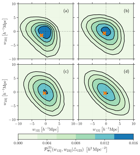
Figure 1: Contour levels for the joint probability distribution of the relative los velocities $w_{12\parallel}$ and $w_{23\parallel}$ extracted from our $N$-body simulation. The mean is indicated with a cross. The four panels correspond to different triangular configurations with $\{r_{12\parallel},r_{12\perp},r_{23\parallel},r_{23\perp},r_{31\perp}\}$ lying within ($5\,h^{-1}$Mpc wide) bins centred at $\{7.5,7.5,7.5,7.5,7.5\}_{(\mathrm{a})}$, $\{27.5,17.5,17.5,17.5,27.5\}_{(\mathrm{b})}$, $\{22.5,32.5,42.5,32.5,27.5\}_{(\mathrm{c})}$, $\{52.5,47.5,57.5,42.5,62.5\}_{(\mathrm{d})}$ in units of $h^{-1}$ Mpc.

We measure ${\mathcal{P}}^{(3)}_{\bm{w}_{\parallel}}(w_{12\parallel},w_{23\parallel}|\triangle_{123})$ from the final output of our $N$-body simulation at $z=0$. This is a demanding task as it requires identifying all particle triplets with a given $r_{12\parallel},r_{12\perp},r_{23\parallel},r_{23\perp}$ and $r_{31\perp}$. herefore, we consider a subsample of $100^{3}$ randomly selected simulation particles. Four examples are shown in figure 1. Note that the distribution is always unimodal with a mode which is close to $(w_{12\parallel},w_{23\parallel})=(0,0)$. On the other hand, the mean los pairwise velocities (indicated with a cross in the plot) are negative. In general, contour levels are not symmetric but tend to become elliptical for large separations. The pairwise velocities $w_{12\parallel}$ and $w_{23\parallel}$ anti-correlate on these scales due to the opposite sign of $v_{2\parallel}$ in their definition.

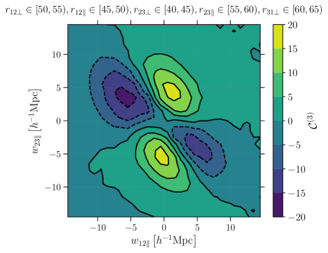
Figure 2: Contour levels for the function ${\mathcal{C}}^{(3)}(w_{12\parallel},w_{23\parallel}|\triangle_{123})$ extracted from our $N$-body simulation by combining several PDFs as in equation (2.35). The side lengths that define the specific triangular configuration we consider are listed on top of the figure in units of $h^{-1}\mathrm{Mpc}$.

In figure 2, we show one example of the function ${\mathcal{C}}^{(3)}(w_{12\parallel},w_{23\parallel}|\triangle_{123})$ for the same triangular configuration considered in the bottom-right panel of figure 1. As expected, ${\mathcal{C}}^{(3)}(w_{12\parallel},w_{23\parallel}|\triangle_{123})$ is more complex than the corresponding ${\mathcal{P}}^{(3)}_{\bm{w}_{\parallel}}(w_{12\parallel},w_{23\parallel}|\triangle_{123})$. The function ${\mathcal{C}}^{(3)}$ shows a typical quadrupolar structure with correlated steps in $w_{12\parallel}$ and $w_{23\parallel}$ giving a positive signal and anti-correlated ones producing a negative output value. Figures 1 and 2 suggest that ${\mathcal{P}}^{(3)}_{\bm{w}_{\parallel}}(w_{12\parallel},w_{23\parallel}|\triangle_{123})$ is best suited for simple approximations in terms of analytical PDFs. We will pursue this phenomenological approach in section 4.

3.3 Moments of ${\mathcal{P}}^{(3)}_{\bm{w}_{\parallel}}(w_{12\parallel},w_{23\parallel}|\triangle_{123})$: perturbative predictions at leading order

In this section, we compute the first two moments of the joint distribution of $w_{12\parallel}$ and $w_{23\parallel}$ using standard perturbation theory at leading order (LO) and compare the results against our simulation.

3.3.1 Mean relative velocities between particle pairs in a triplet

Standard perturbation theory assumes that the matter content of the Universe is in the single-stream regime and, at any given time, describes it in terms of two continuous fields: the mass density contrast $\delta(\bm{x})$ and the peculiar velocity $\bm{u}(\bm{x})$. Linear perturbations in $\delta$ grow proportionally to the growth factor $D$ while those in $\bm{u}$ grow proportionally to $aHfD$ with $f=\mathrm{d}\log D/\mathrm{d}\log a$. The Fourier transforms of the linear terms are related as

$$\tilde{\bm{u}}(\bm{k})=aHf\,\frac{i\bm{k}}{k^{2}}\,\tilde{\delta}(\bm{k})\;.$$ (3.1)

To make equations shorter, we follow the notation introduced in sections 2.1 and 2.6 and describe peculiar velocities in terms of the vector field $\mathsf{v}(\bm{x})=\bm{u}(\bm{x})/(aH)$, i.e. in terms of the comoving separation vector that gives rise to a Hubble velocity $\bm{u}$. However, we continue referring to $\mathsf{v}$ as a velocity.

Let us consider the mean pairwise (relative) velocity

$$\langle\bm{w}_{12}|\bm{r}_{12}\rangle_{\mathrm{p}}=\int\bm{w}_{12}\,\mathcal{P}^{(2)}_{\bm{w}_{12}}(\bm{w}_{12}|\bm{r}_{12})\,\mathrm{d}\bm{w}_{12}\,,$$ (3.2)

where the subscript p indicates a pair-weighted average, i.e. an average taken over all particle pairs with separation $\bm{r}_{12}$, and $\mathcal{P}^{(2)}_{\bm{w}_{12}}$ generalises equation (2.39) to the full vector $\bm{w}_{12}$. In the single-stream regime, since the number of particles at one location is proportional to $1+\delta$ (see section 2.6), we can write

$$\langle\bm{w}_{12}|\bm{r}_{12}\rangle_{\mathrm{p}}=\displaystyle\frac{\langle(1+\delta_{1})(1+\delta_{2})(\bm{v}_{2}-\bm{v}_{1})\rangle}{\langle(1+\delta_{1})(1+\delta_{2})\rangle}\;,$$ (3.3)

where $\delta_{i}$ and $\bm{v}_{i}$ are short for $\delta(\bm{x}_{i})$ and $\mathsf{v}(\bm{x}_{i})$. At LO in the perturbations, $\langle\bm{w}_{12}|\bm{r}_{12}\rangle_{\mathrm{p}}\simeq\langle\delta_{1}\bm{v}_{2}\rangle-\langle\delta_{2}\bm{v}_{1}\rangle$ and, making use of equation (3.1), it is straightforward to show that

$$\langle\delta_{1}\bm{v}_{2}\rangle=-\frac{f}{2\pi^{2}}\,\hat{\bm{r}}_{12}\int_{0}^{\infty}\!\!\!\!k\,j_{1}(k\,r_{12})\,P(k)\,\mathrm{d}k\,,$$ (3.4)

where $j_{1}(x)=\sin(x)/x^{2}-\cos(x)/x$, and $P(k)$ denotes the linear matter power spectrum. Putting everything together, one obtains [6]

$$\langle\bm{w}_{12}|\bm{r}_{12}\rangle_{\mathrm{p}}\simeq\displaystyle-\frac{f}{\pi^{2}}\,\hat{\bm{r}}_{12}\int_{0}^{\infty}\!\!\!\!k\,j_{1}(k\,r_{12})\,P(k)\,\mathrm{d}k=\bar{w}(r_{12})\,\hat{\bm{r}}_{12}\,,$$ (3.5)

where the symbol $\simeq$ indicates that the expression has been truncated to LO. Note that, because of gravity, the particles in a pair approach each other on average, i.e. $\bar{w}(r_{12})<0$.

We now want to generalise this calculation to particle triplets with separations $\triangle_{123}=(\bm{r}_{12},\bm{r}_{23},\bm{r}_{31})$. In this case, there are three mean relative velocities to consider: $\langle\bm{w}_{12}|\triangle_{123}\rangle_{\mathrm{t}}$, $\langle\bm{w}_{23}|\triangle_{123}\rangle_{\mathrm{t}}$, and $\langle\bm{w}_{31}|\triangle_{123}\rangle_{\mathrm{t}}$ (the subscript t, here, denotes that averages are taken over all particle triplets with separations $\triangle_{123}$). For instance, to LO in the perturbations,

$$\langle\bm{w}_{12}|\triangle_{123}\rangle_{\mathrm{t}}= \displaystyle\frac{\langle(1+\delta_{1})(1+\delta_{2})(1+\delta_{3})(\bm{v}_{2}-\bm{v}_{1})\rangle}{\langle(1+\delta_{1})(1+\delta_{2})(1+\delta_{3})\rangle}$$

$$\simeq \langle\delta_{1}\bm{v}_{2}\rangle-\langle\delta_{2}\bm{v}_{1}\rangle+\langle\delta_{3}\bm{v}_{2}\rangle-\langle\delta_{3}\bm{v}_{1}\rangle$$

$$= \bar{w}(r_{12})\,\hat{\bm{r}}_{12}-\frac{1}{2}\left[\bar{w}(r_{23})\,\hat{\bm{r}}_{23}+\bar{w}(r_{31})\,\hat{\bm{r}}_{31}\right]\,.$$ (3.6)

Note that the mean relative velocity between a particle pair in a triplet is not purely radial but has also a transverse component in the plane of the triangle defined by the particles. This is generated by the gravitational influence of the third particle on the pair. In order to separate the radial and transverse components, let us first denote by $\chi=\arccos(\hat{\bm{r}}_{12}\cdot\hat{\bm{r}}_{23})$ the (shortest) rotation angle from $\hat{\bm{r}}_{12}$ to $\hat{\bm{r}}_{23}$ around the normal vector $\bm{n}=\hat{\bm{r}}_{12}\times\hat{\bm{r}}_{23}=\hat{\bm{n}}\,\sin\chi$ (with $0\leq\chi<\pi$ and $\sin\chi\geq 0$). We then build a right-handed Cartesian coordinate system with unit axes $\{\hat{\bm{r}}_{12},\hat{\bm{t}},\hat{\bm{n}}\}$ such that $\hat{\bm{t}}=\hat{\bm{n}}\times\hat{\bm{r}}_{12}=(\hat{\bm{r}}_{23}-\cos\chi\,\hat{\bm{r}}_{12})/\sin\chi$ (see also appendix A in [53]). By construction, $\hat{\bm{t}}$ lies in the plane of $\triangle_{123}$, is orthogonal to $\hat{\bm{r}}_{12}$, and always points towards the half-plane that contains point 3 with respect to the $\hat{\bm{r}}_{12}$ direction. Since $\bm{r}_{12}+\bm{r}_{23}+\bm{r}_{31}=0$, it follows that $\bm{r}_{31}\cdot\hat{\bm{r}}_{12}=-(r_{12}+r_{23}\,\cos\chi)$ and $\bm{r}_{31}\cdot\hat{\bm{t}}=-r_{23}\,\sin\chi$. We can thus decompose the mean relative velocity between a particle pair in a triplet into its radial and transverse components (by symmetry, there cannot be any component along $\hat{\bm{n}}$ as motions in the two vertical directions are equally likely)

$$\langle\bm{w}_{12}|\triangle_{123}\rangle_{\mathrm{t}} =\langle\bm{w}_{12}\cdot\hat{\bm{r}}_{12}|\triangle_{123}\rangle_{\mathrm{t}}\,\hat{\bm{r}}_{12}+\langle\bm{w}_{12}\cdot\hat{\bm{t}}|\triangle_{123}\rangle_{\mathrm{t}}\,\hat{\bm{t}}$$

$$=R_{12}(\triangle_{123})\,\hat{\bm{r}}_{12}+T_{12}(\triangle_{123})\,\hat{\bm{t}}\;,$$ (3.7)

obtaining

$$R_{12}(\triangle_{123})=\bar{w}(r_{12})-\frac{1}{2}\left[\bar{w}(r_{23})\,\cos\chi-\bar{w}(r_{31})\,\frac{r_{12}+r_{23}\cos\chi}{\sqrt{r_{12}^{2}+r_{23}^{2}+2r_{12}r_{23}\cos\chi}}\right]\;,$$ (3.8)

$$T_{12}(\triangle_{123})=-\frac{1}{2}\left[\bar{w}(r_{23})-\bar{w}(r_{31})\,\frac{r_{23}}{\sqrt{r_{12}^{2}+r_{23}^{2}+2r_{12}r_{23}\cos\chi}}\right]\,\sin\chi\;,$$ (3.9)

where we have parameterized the shape of $\triangle_{123}$ in terms of $r_{12},r_{23}$ and $\chi$ (since $r_{31}^{2}=r_{12}^{2}+r_{23}^{2}+2r_{12}r_{23}\cos\chi$ and $\sin\chi=\sqrt{1-\cos^{2}\chi}$ it is straightforward to use the three side lengths instead). Equations (3.8) and (3.9) describe how the presence of the third particle influences the mean radial velocity in a pair and gives rise to a transverse component. Depending on the exact geometrical configuration, $R_{12}(\triangle_{123})$ can be larger or smaller than $\bar{w}(r_{12})$ and $T_{12}(\triangle_{123})$ positive or negative. If $\bm{r}_{12}$ is the base of an isosceles triangle, for instance, then $R_{12}=\bar{w}(r_{12})+\bar{w}(r_{23})(r_{12}/r_{31})/2$ and $T_{12}=0$. This reflects the fact that the ‘gravitational pulls’ due to the third particle add up to generate a larger relative velocity in the radial direction but exactly cancel out in the transverse one. For equilateral triangles, this reduces to $R_{12}=3\bar{w}(r_{12})/2$ and $T_{12}=0$. Considering a degenerate triangle with $\chi=0$ gives $R_{12}=\bar{w}(r_{12})-[\bar{w}(r_{23})-\bar{w}(r_{31})]/2$ and $T_{12}=0$. A note is in order here. Triangles with the same shape can have opposite orientations (intended as winding orders, i.e. signed areas of opposite signs) and both $\hat{\bm{t}}$ and $\hat{\bm{n}}$ flip sign if the winding order of $\triangle_{123}$ is switched (e.g. by reflecting the triangle with respect to $\bm{r}_{12}$). It follows that, if one disregards orientation and takes the average among all triangles with given side lenghts, then the transverse part of the mean relative velocity between a particle pair in a triplet is a null vector as triangles with opposite winding orders give identical contributions in opposite directions. As stated in equation (3.7), with the term ‘transverse component’ we always refer to the projection along $\hat{\bm{t}}$ which does not vanish even when the average is taken irrespective of orientation.

The steps above can be repeated to decompose $\langle\bm{w}_{23}|\triangle_{123}\rangle_{\mathrm{t}}$ in its radial and transverse parts. In this case, we use a right-handed coordinate system with unit axes $\{\hat{\bm{r}}_{23},\hat{\bm{t}}^{\prime},\hat{\bm{n}}\}$ where $\hat{\bm{t}}^{\prime}=\hat{\bm{n}}\times\hat{\bm{r}}_{23}=(-\hat{\bm{r}}_{12}+\cos\chi\,\hat{\bm{r}}_{23})/\sin\chi$) and write $\langle\bm{w}_{23}|\triangle_{123}\rangle_{\mathrm{t}}=R_{23}(\triangle_{123})\,\hat{\bm{r}}_{23}+T_{23}(\triangle_{123})\,\hat{\bm{t}}^{\prime}$. The resulting radial and transverse components are, respectively,

$$R_{23}(\triangle_{123})=\bar{w}(r_{23})-\frac{1}{2}\left[\bar{w}(r_{12})\,\cos\chi-\bar{w}(r_{31})\,\frac{r_{23}+r_{12}\cos\chi}{\sqrt{r_{12}^{2}+r_{23}^{2}+2r_{12}r_{23}\cos\chi}}\right]\;,$$ (3.10)

$$T_{23}(\triangle_{123})=\frac{1}{2}\left[\bar{w}(r_{12})-\bar{w}(r_{31})\,\frac{r_{12}}{\sqrt{r_{12}^{2}+r_{23}^{2}+2r_{12}r_{23}\cos\chi}}\right]\,\sin\chi\;.$$ (3.11)

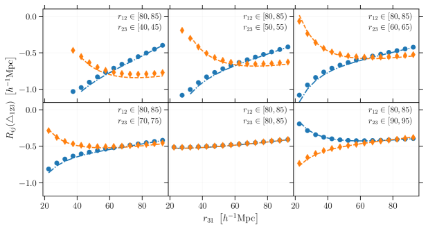
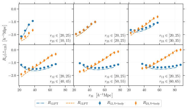
Figure 3: The radial component of the mean relative velocity between particle pairs in a triplet for different triangular configurations. Symbols with error bars denote measurements from our $N$-body simulation while the smooth curves show the predictions from the perturbative calculations at LO derived in section 3.3.1. The labels give the particle separations $r_{12}$ and $r_{23}$ in units of $h^{-1}\mathrm{Mpc}$.

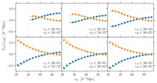
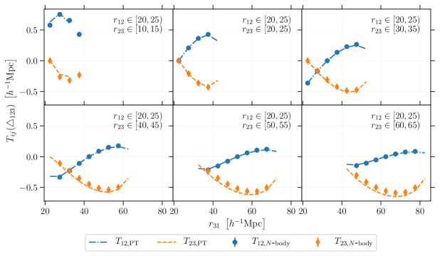
Figure 4: As in figure 3 but for the transverse component.

In figures 3 and 4, we compare the perturbative results at LO for $R_{12}$, $R_{23}$, $T_{12}$ and $T_{23}$ against measurements from the simulation introduced in section 3.1. We consider triangular configurations $\triangle_{123}$ with different shapes and sizes (but we always average over winding order). In the top set of panels, we look at triangles with relatively large values of $r_{12}$ and $r_{23}$. Here, $r_{12}\in[80,85)\,h^{-1}\mathrm{Mpc}$ and each sub panel corresponds to a different narrow range for $r_{23}$ as indicated by the labels. Results are plotted as a function of $r_{31}$ (i.e. by varying $\chi$). It is remarkable to see that the theoretical predictions match very well the measurements from the simulation for these large triangles. In the bottom set of panels, we consider smaller triangles with $r_{12}\in[20,25)\,h^{-1}\mathrm{Mpc}$ and also smaller values for $r_{23}$. Also in this case, the LO predictions are quite accurate although to a lesser degree than in the top panel. We conclude that the perturbative calculations are a reliable tool to compute the mean relative velocity for triangular configurations with scales $r\gtrsim 20\,h^{-1}\mathrm{Mpc}$).

3.3.2 Dispersion of relative velocities between particle pairs in a triplet

The second moment of the pairwise velocity

$$\langle\bm{w}_{12}\,\bm{w}_{12}|\bm{r}_{12}\rangle_{\mathrm{p}}= \displaystyle\frac{\langle(1+\delta_{1})(1+\delta_{2})(\bm{v}_{2}-\bm{v}_{1})(\bm{v}_{2}-\bm{v}_{1})\rangle}{\langle(1+\delta_{1})(1+\delta_{2})\rangle}$$ (3.12)

is a dyadic tensor which, to LO in the perturbations, reduces to

$$\langle\bm{w}_{12}\,\bm{w}_{12}|\bm{r}_{12}\rangle_{\mathrm{p}}\simeq\langle\bm{v}_{2}\bm{v}_{2}\rangle-\langle\bm{v}_{2}\bm{v}_{1}\rangle-\langle\bm{v}_{1}\bm{v}_{2}\rangle+\langle\bm{v}_{1}\bm{v}_{1}\rangle\;.$$ (3.13)

Two-point correlations between linear velocity fields are conveniently written as [77]

$$\langle v_{1i}\,v_{2j}\rangle\simeq\psi_{p}(r_{12})\,\delta_{ij}+[\psi_{r}(r_{12})-\psi_{p}(r_{12})]\,\hat{r}_{12i}\,\hat{r}_{12j}\;,$$ (3.14)

where the indices $i$ and $j$ denote the Cartesian components of the velocities (i.e. they run from 1 to 3), $\delta_{ij}$ is the Kronecker symbol, and $\psi_{r}$ and $\psi_{p}$ are the radial and transverse correlation functions defined as

$$\psi_{r}(r_{12})=\displaystyle\frac{f^{2}}{2\pi^{2}}\int_{0}^{\infty}\Biggl{[}j_{0}(k\,r_{12})-2\,\frac{j_{1}(k\,r_{12})}{k\,r_{12}}\Biggr{]}\,P(k)\,\mathrm{d}k\;,$$ (3.15)

$$\psi_{p}(r_{12})=\displaystyle\frac{f^{2}}{2\pi^{2}}\int_{0}^{\infty}\frac{j_{1}(k\,r_{12})}{k\,r_{12}}\,P(k)\,\mathrm{d}k\;,$$ (3.16)

with $j_{0}(x)=\sin(x)/x$. Note that, when $r_{12}\to 0$, $\psi_{p}\to\sigma^{2}_{v}$ and $\psi_{r}\to\sigma^{2}_{v}$ where

$$\sigma^{2}_{v}=\frac{f^{2}}{6\pi^{2}}\int_{0}^{\infty}\!\!\!\!P(k)\,\mathrm{d}k$$ (3.17)

is the one-dimensional linear velocity dispersion, i.e. $\sigma_{v}^{2}=\langle v_{i}^{2}\rangle$. Therefore, the velocity dispersion tensor at zero lag is isotropic

$$\langle v_{1i}\,v_{1j}\rangle=\langle v_{2i}\,v_{2j}\rangle=\sigma^{2}_{v}\,\delta_{ij}\;.$$ (3.18)

It follows that

$$\langle w_{12i}\,w_{12j}|\bm{r}_{12}\rangle_{\mathrm{p}}\simeq 2\left[\sigma_{v}^{2}-\psi_{p}(r_{12})\right]\,\delta_{ij}-2\left[\psi_{r}(r_{12})-\psi_{p}(r_{12})\right]\,\hat{r}_{12i}\,\hat{r}_{12j}\;.$$ (3.19)

In other words, the second moments of the radial component is

$$\langle(\bm{w}_{12}\cdot\hat{\bm{r}}_{12})^{2}|\bm{r}_{12}\rangle_{\mathrm{p}}=2\left[\sigma^{2}_{v}-\psi_{r}(r_{12})\right]\;,$$ (3.20)

while for each of the perpendicular components (e.g. those along the unit vectors $\hat{\bm{n}}$ and $\hat{\bm{t}}$ introduced in section 3.3.1) we have

$$\frac{1}{2}\langle[\bm{w}_{12}-(\bm{w}_{12}\cdot\hat{\bm{r}}_{12})\hat{\bm{r}}_{12}]^{2}|\bm{r}_{12}\rangle_{\mathrm{p}}=2\left[\sigma^{2}_{v}-\psi_{p}(r_{12})\right]\;.$$ (3.21)

Moreover, the different Cartesian components are uncorrelated.

The calculations above can be easily extended to particle pairs in a triplet. In this case, we are interested in two types of combinations, e.g.

$$\langle\bm{w}_{12}\,\bm{w}_{12}|\triangle_{123}\rangle_{\mathrm{t}}= \displaystyle\frac{\langle(1+\delta_{1})(1+\delta_{2})(1+\delta_{3})(\bm{v}_{2}-\bm{v}_{1})(\bm{v}_{2}-\bm{v}_{1})\rangle}{\langle(1+\delta_{1})(1+\delta_{2})(1+\delta_{3})\rangle}\;,$$ (3.22)

and

$$\langle\bm{w}_{12}\,\bm{w}_{23}|\triangle_{123}\rangle_{\mathrm{t}}= \displaystyle\frac{\langle(1+\delta_{1})(1+\delta_{2})(1+\delta_{3})(\bm{v}_{2}-\bm{v}_{1})(\bm{v}_{3}-\bm{v}_{2})\rangle}{\langle(1+\delta_{1})(1+\delta_{2})(1+\delta_{3})\rangle}\;.$$ (3.23)

To LO in the perturbations, they reduce to

$$\langle\bm{w}_{12}\,\bm{w}_{12}|\triangle_{123}\rangle_{\mathrm{t}}\simeq \langle\bm{v}_{2}\bm{v}_{2}\rangle-\langle\bm{v}_{2}\bm{v}_{1}\rangle-\langle\bm{v}_{1}\bm{v}_{2}\rangle+\langle\bm{v}_{1}\bm{v}_{1}\rangle\;,$$ (3.24)

and

$$\langle\bm{w}_{12}\,\bm{w}_{23}|\triangle_{123}\rangle_{\mathrm{t}}\simeq \langle\bm{v}_{2}\bm{v}_{3}\rangle-\langle\bm{v}_{2}\bm{v}_{2}\rangle-\langle\bm{v}_{1}\bm{v}_{3}\rangle+\langle\bm{v}_{1}\bm{v}_{2}\rangle\;.$$ (3.25)

that have exactly the same structure as equation (3.14). Therefore, we conclude that

$$\langle w_{12i}\,w_{12j}|\triangle_{123}\rangle_{\mathrm{t}}\simeq 2\left[\sigma_{v}^{2}-\psi_{p}(r_{12})\right]\,\delta_{ij}-2\left[\psi_{r}(r_{12})-\psi_{p}(r_{12})\right]\,\hat{r}_{12i}\,\hat{r}_{12j}\;,$$ (3.26)

and

$$\langle w_{12i}\,w_{23j}|\triangle_{123}\rangle_{\mathrm{t}}\simeq \left[\psi_{p}(r_{12})+\psi_{p}(r_{23})-\psi_{p}(r_{31})-\sigma^{2}_{v}\right]\,\delta_{ij}$$

$$+\left[\psi_{r}(r_{12})-\psi_{p}(r_{12})\right]\,\hat{r}_{12i}\,\hat{r}_{12j}$$

$$+\left[\psi_{r}(r_{23})-\psi_{p}(r_{23})\right]\,\hat{r}_{23i}\,\hat{r}_{23j}$$

$$-\left[\psi_{r}(r_{31})-\psi_{p}(r_{31})\right]\,\hat{r}_{31i}\,\hat{r}_{31j}\;.$$ (3.27)

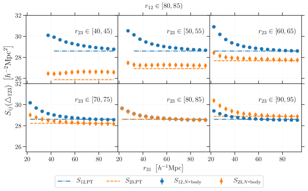
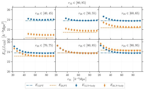
Figure 5: As in the top panel of figure 3 but for the second moment of the radial (top) and transverse (bottom) components of the relative velocity between particle pairs in a triplet. Note that a constant offset has been added to the theoretical predctions as described at the end of section 3.3.2.

In figure 5, we compare some of these perturbative results to measurements performed in our numerical simulation. Shown are the second moments of the radial (top panel) and transverse (bottom panel) components of the relative velocity between particle pairs in a triplet. Symbols with error bars display the $N$-body measurements while the constant lines indicate the theoretical results to LO, i.e,

$$S_{12}(\triangle_{123})=\langle(\bm{w}_{12}\cdot\hat{\bm{r}}_{12})^{2}|\triangle_{123}\rangle_{\mathrm{t}} =2\left[\sigma^{2}_{v}-\psi_{r}(r_{12})\right]\;,$$ (3.28)

$$E_{12}(\triangle_{123})=\langle(\bm{w}_{12}\cdot\hat{\bm{t}})^{2}|\triangle_{123}\rangle_{\mathrm{t}} =2\left[\sigma^{2}_{v}-\psi_{p}(r_{12})\right]\;,$$ (3.29)

and the corresponding results for $\bm{w}_{23}$. The first thing worth mentioning is that the second moments are generally much larger than the mean values shown in figures. 3 and 4. The model, however, does not account for all the dispersion around the mean. In fact, as previously noted in the literature [7, 78, 17], the prediction for $\sigma^{2}_{v}$ given in equation (3.17) is not very accurate. Being a zero-lag correlation, $\sigma^{2}_{v}$ is influenced by small-scale, non-perturbative physics. Adding a constant offset to equations (3.28) and (3.29) is a common fix that has been found to reproduce simulations well. We follow this approach and add a constant $C$ to $\sigma_{v}^{2}$ so that to match the measurements for the largest triangles we consider (i.e. the rightmost points in the bottom-right sub panels). This way, we find consistent offset values ($C\simeq 4.8\,h^{-2}\mathrm{Mpc}^{2}$ within 1%) for the dispersions in the radial and transverse components as well as in the pairwise velocity. Keeping this shift fixed, we find that the theoretical predictions are able to reproduce the measurements from the simulation quite well for the largest triangles. However, the level of agreement drops off rapidly when lower separation scales are considered.

3.3.3 Projection along the line of sight

The los component of the relative velocities between particle pairs in a triplet depends on the relative orientation of $\triangle_{123}$ with respect to the los (see Appendix A in [53] for a detailed discussion). We set up a spherical coordinate system with $\hat{\bm{r}}_{12}$ as the polar axis and use $\theta=\arccos(\hat{\bm{r}}_{12}\cdot\hat{\bm{s}})$ as the polar angle ($0\leq\theta<\pi$). We also define the azimuthal angle $\phi$ ($0\leq\phi<2\pi$) as the angle between $\hat{\bm{n}}$ and the projection of $\hat{\bm{s}}$ on to the plane perpendicular to $\hat{\bm{r}}_{12}$ so that $\cos\phi=0$ whenever $\hat{\bm{s}}$ lies in the plane of the triangle. It follows that $\hat{\bm{t}}\cdot\hat{\bm{s}}=\sin\theta\sin\phi$, $\hat{\bm{n}}\cdot\hat{\bm{s}}=\sin\theta\cos\phi$, and $\hat{\bm{t}}^{\prime}\cdot\hat{\bm{s}}=-\cos\theta\sin\chi+\sin\theta\sin\phi\cos\chi$. For the scalar products between the different pairwise separation vectors and the los direction, one thus finds [67, 53],

$$\mu_{12}=\hat{\bm{r}}_{12}\cdot\hat{\bm{s}}=\frac{r_{12\parallel}}{r_{12}}=\cos\theta\;,$$ (3.30)

$$\mu_{23}=\hat{\bm{r}}_{23}\cdot\hat{\bm{s}}=\frac{r_{23\parallel}}{r_{23}}=\cos\theta\cos\chi+\sin\theta\sin\phi\sin\chi\;,$$ (3.31)

$$\mu_{31}=\hat{\bm{r}}_{31}\cdot\hat{\bm{s}}=\frac{-(r_{12\parallel}+r_{23\parallel})}{r_{31}}=-\frac{r_{12}}{r_{31}}\mu_{12}-\frac{r_{23}}{r_{31}}\mu_{23}\;.$$ (3.32)

Note that by flipping the winding order of $\triangle_{123}$ for a fixed los direction, $\cos\theta$ stays the same while both $\sin\phi$ and $\cos\phi$ change sign (i.e. $\phi\to\pi+\phi\mod 2\pi$) as $\hat{\bm{t}}$ and $\hat{\bm{n}}$ flip.

Combining equations (3.30), (3.31) and (3.32) with the results obtained in section 3.3, we can eventually write the first and second moments for the projections of the relative velocities along the los, $w_{12\parallel}$ and $w_{23\parallel}$. In particular, equation (3.6) gives

$$\langle w_{12\parallel}|\triangle_{123}\rangle_{\mathrm{t}}\simeq\bar{w}(r_{12})\,\mu_{12}-\frac{1}{2}\left[\bar{w}(r_{23})\,\mu_{23}+\bar{w}(r_{31})\,\mu_{31}\right]\;.$$ (3.33)

The very same expression can be derived from equation (3.7) and written as

$$\langle w_{12\parallel}|\triangle_{123}\rangle_{\mathrm{t}}\simeq R_{12}(\triangle_{123})\,\cos\theta+T_{12}(\triangle_{123})\,\sin\theta\sin\phi\;.$$ (3.34)

Similarly, we have

$$\langle w_{23\parallel}|\triangle_{123}\rangle_{\mathrm{t}}\simeq\bar{w}(r_{23})\,\mu_{23}-\frac{1}{2}\left[\bar{w}(r_{12})\,\mu_{12}+\bar{w}(r_{31})\,\mu_{31}\right]\;,$$ (3.35)

and

$$\langle w_{23\parallel}|\triangle_{123}\rangle_{\mathrm{t}}\simeq R_{23}(\triangle_{123})\,\mu_{23}+T_{23}(\triangle_{123})\,(-\cos\theta\sin\chi+\sin\theta\sin\phi\cos\chi)\;.$$ (3.36)

Moreover, from equation (3.26) we derive

$$\langle w_{12\parallel}^{2}|\triangle_{123}\rangle_{\mathrm{t}} \simeq 2\left[\sigma_{v}^{2}-\psi_{p}(r_{12})\right]-2\left[\psi_{r}(r_{12})-\psi_{p}(r_{12})\right]\,\mu_{12}^{2}$$

$$=2\left[\sigma_{v}^{2}-\psi_{\parallel}(r_{12})\right]\;,$$ (3.37)

with $\psi_{\parallel}(r_{12})=\mu^{2}_{12}\,\psi_{r}(r_{12})+(1-\mu^{2}_{12})\,\psi_{p}(r_{12})$. The corresponding expression for $\langle w_{23\parallel}^{2}|\triangle_{123}\rangle_{\mathrm{t}}$ is obtained by replacing $r_{12}$ with $r_{23}$ in equation (3.37). Finally, equation (3.27) implies

$$\langle w_{12\parallel}\,w_{23\parallel}|\triangle_{123}\rangle_{\mathrm{t}}\simeq \left[\psi_{p}(r_{12})+\psi_{p}(r_{23})-\psi_{p}(r_{31})-\sigma^{2}_{v}\right]\,$$

$$+\left[\psi_{r}(r_{12})-\psi_{p}(r_{12})\right]\,\mu_{12}^{2}$$

$$+\left[\psi_{r}(r_{23})-\psi_{p}(r_{23})\right]\,\mu_{23}^{2}$$

$$-\left[\psi_{r}(r_{31})-\psi_{p}(r_{31})\right]\,\mu_{31}^{2}$$

$$= \,\,\psi_{\parallel}(r_{12})+\psi_{\parallel}(r_{23})-\psi_{\parallel}(r_{31})-\sigma^{2}_{v}\;.$$ (3.38)

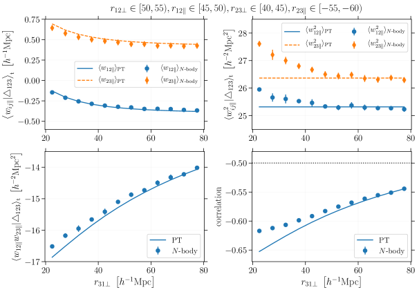
Figure 6: Moments of the relative los velocities between particle pairs in a triplet, $w_{12\parallel}$ and $w_{23\parallel}$. The mean values (top left), the second moments (top right), the second cross moment (bottom left), and the linear correlation coefficient (bottom right) are plotted for different triangular configurations $\triangle_{123}$. Symbols with error bars denote measurements from our $N$-body simulation while the smooth curves show the predictions from the perturbative calculations at LO derived in section 3.3.3. The labels give the particle separations in units of $h^{-1}\mathrm{Mpc}$.

We compare these results with measurements from the simulation in figure 6. In this case, we bin our data based on the variables:

$$r_{12\parallel} =r_{12}\,\cos\theta\;,$$

$$r_{12\perp} =r_{12}\,|\sin\theta|\;,$$

$$r_{23\parallel} =r_{23}\,(\cos\theta\cos\chi+\sin\theta\sin\phi\sin\chi)\;,$$ (3.39)

$$r_{23\perp} =r_{23}\,[1-(\cos\theta\cos\chi+\sin\theta\sin\phi\sin\chi)^{2}]^{1/2}\;,$$

$$r_{31\perp} =\left\{r_{12}^{2}+r_{23}^{2}+2r_{12}r_{23}\cos\chi-\left[r_{12}\cos\theta+r_{23}\,(\cos\theta\cos\chi+\sin\theta\sin\phi\sin\chi)\right]^{2}\right\}^{1/2}\;,$$

(note that triangles with the same shape but opposite winding orders correspond to different sets of these variables). Results are plotted as a function of $r_{31\perp}$ by keeping the remaining four variables that define a triangular configuration fixed. The top-left panel shows $\langle w_{12\parallel}|\triangle_{123}\rangle_{\mathrm{t}}$ and $\langle w_{23\parallel}|\triangle_{123}\rangle_{\mathrm{t}}$. Here, the theoretical predictions are in very good agreement with the numerical data confirming the results presented in figures  3 and 4. The top-right panel displays $\langle w_{12\parallel}^{2}|\triangle_{123}\rangle_{\mathrm{t}}$ and $\langle w_{23\parallel}^{2}|\triangle_{123}\rangle_{\mathrm{t}}$ while the bottom-left panel shows $\langle w_{12\parallel}\,w_{23\parallel}|\triangle_{123}\rangle_{\mathrm{t}}$. Once adjusted for the offset discussed in section 3.3.2, the predictions for the second moments are excellent for $r_{31\perp}\gtrsim 50\,h^{-1}\ \mathrm{Mpc}$ but tend to slightly underestimate the $N$-body results by a few percent at smaller separations. Likewise, the model for the cross second moment always agrees to better than 3% with the simulation and gives better predictions when $r_{31\perp}$ is large. Note that the linear correlation coefficient between $w_{12\parallel}$ and $w_{23\parallel}$ (bottom-right panel) is always close to $-1/2$ as expected from drawing independent los velocities from $\mathcal{P}^{(1)}_{v_{\parallel}}$ at every vertex of $\triangle_{123}$ (see also figure 1 and the detailed discussion in section 4.4).

4 The 3-point Gaussian streaming model

4.1 Definitions

The streaming model for the 3PCF given in equation (2.18) is exact within the distant-observer approximation. However, it requires knowledge of the function ${\mathcal{P}}^{(3)}_{\bm{w}_{\parallel}}(w_{12\parallel},w_{23\parallel}|\triangle_{123})$ which is challenging to derive from first principles. In analogy to the literature on the 2-point correlation function, we propose the use of a scale-dependent bivariate Gaussian distribution to model ${\mathcal{P}}^{(3)}_{\bm{w}_{\parallel}}(w_{12\parallel},w_{23\parallel}|\triangle_{123})$. This choice is motivated by a number of considerations: i) For large inter-particle separations, the function ${\mathcal{P}}^{(3)}_{\bm{w}_{\parallel}}(w_{12\parallel},w_{23\parallel}|\triangle_{123})$ extracted from our simulation appears to be approximately Gaussian close to its peak (e.g. see the bottom right panel in figure 1); ii) Simplicity, as the Gaussian is the only probability density function that only requires two cumulants to be fully specified; iii) As shown in section 3.3, on large scales, we can accurately model the scale dependence of these cumulants by using perturbation theory at LO.

In the resulting phenomenological model, which we dub the ‘3-point Gaussian streaming model’ (3ptGSM in short), the joint probability density function of $w_{12\parallel}$ and $w_{23\parallel}$ is given by a bivariate Gaussian distribution with mean values $m_{1}=\langle w_{12\parallel}|\triangle_{123}\rangle_{\mathrm{t}}$, $m_{2}=\langle w_{23\parallel}|\triangle_{123}\rangle_{\mathrm{t}}$ and covariance matrix with elements $C_{11}=\langle w_{12\parallel}^{2}|\triangle_{123}\rangle_{\mathrm{t}}-\langle w_{12\parallel}|\triangle_{123}\rangle_{\mathrm{t}}^{2}$, $C_{12}=C_{21}=\langle w_{12\parallel}\,w_{23\parallel}|\triangle_{123}\rangle_{\mathrm{t}}-\langle w_{12\parallel}|\triangle_{123}\rangle_{\mathrm{t}}\langle w_{23\parallel}|\triangle_{123}\rangle_{\mathrm{t}}$, $C_{22}=\langle w_{23\parallel}^{2}|\triangle_{123}\rangle_{\mathrm{t}}-\langle w_{23\parallel}|\triangle_{123}\rangle_{\mathrm{t}}^{2}$.

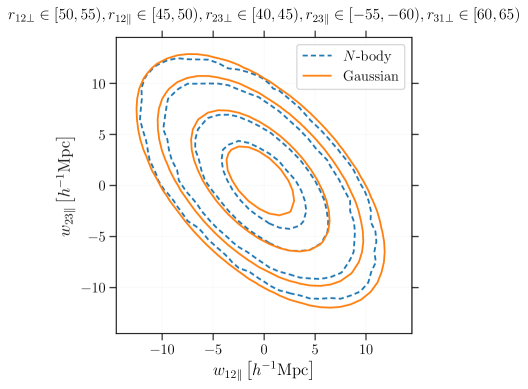
Figure 7: Contour levels of the joint PDF ${\mathcal{P}}^{(3)}_{\bm{w}_{\parallel}}(w_{12\parallel},w_{23\parallel}|\triangle_{123})$ extracted from our $N$-body simulation (dashed) are compared with those of the Gaussian model (solid) with cumulants predicted from perturbation theory at LO. The triangular configuration we consider is specified in the label on top of the figure in units of $h^{-1}\mathrm{Mpc}$. Contours correspond to the levels $\{6,3,1,0.4\}\times 10^{-3}$ with the values decreasing from inside to outside.

In what follows, we investigate the simplest possible implementation of the 3ptGSM based on the perturbative predictions at LO given in equations (3.33), (3.35), (3.37), and (3.38). In figure 7, we compare the resulting PDF with that extracted from our simulation for a particular triangular configuration which is specified on top of the figure. To first approximation, the Gaussian model provides a very good description of the PDF. Looking into more details reveals that it slightly underestimates the probability density around the peak. The Kullback-Leibler (KL) and the Jensen-Shannon (JS) divergences are 0.028 and 0.005 nats, respectively, indicating that the information loss associated with using the Gaussian approximation in place of the actual PDF is minimal. Similar values are obtained for different triangular configurations on large scales. However, the approximation clearly fails at smaller separations as is evident visually from figure 1. In this case, for the triangular configuration considered in the top-left panel, we find KL and JS divergences of 1.31 nats and 0.39 nats (the upper bound being $\ln(2)\simeq 0.69$ nats), respectively.

4.2 3-point correlations in the $N$-body simulation

Our plan is to test the predictions of the 3ptGSM against our $N$-body simulation. In order to measure $\mathcal{G}_{3}$, we first generate catalogs of ‘random’ particles with uniform density within the simulation box and then use the ‘natural’ estimator $DDD/RRR$ where the symbols $DDD$ and $RRR$ denote the normalised data-data-data and random-random-random triplet counts in a bin of triangular configurations, respectively [21, 5]. We characterize the shape and orientation of each triplet using the five-dimensional space $(s_{12\perp},s_{12\parallel},s_{23\perp},s_{23\parallel},s_{31\perp})$ and, for all separations, we use bins that are $5\,h^{-1}$ Mpc wide. To speed the calculation up, we analyse ten subsamples of $100^{3}$ particles each randomly selected from the simulation. For each subsample, we employ five random catalogs containing $1.5\times 100^{3}$ objects each to measure $RRR$. Our final estimates for $\mathcal{G}_{3}$ are obtained by averaging the partial results from the ten subsamples. Error bars are computed by resampling the measurements from the different subsamples with the bootstrap method. Since measuring the 3PCFs is very time consuming and perturbation theory is only expected to be accurate on large-enough scales, we consider a limited number of triangular configurations with fixed $s_{12\perp}\in[50,55)\,h^{-1}$ Mpc and $s_{23\perp}\in[40,45)\,h^{-1}$ Mpc. We vary $s_{12\parallel}$, $s_{23\parallel}$ in the range $[15,65)\,h^{-1}$ Mpc and $s_{31\perp}$ between 25 and $80\,h^{-1}$ Mpc. We present some examples of our results in figure 8 and discuss them in detail in section 4.3.

We also measure the connected 3PCF using the Szapudi-Szalay estimator that we schematically write as $(D-R)(D-R)(D-R)/RRR$ [82, 81]. We implement three versions of the estimator for the 3PCF obtained by binning the triplet counts in different ways.

1. To begin with, we consider the same binning scheme in five dimensions we have used to measure ${\mathcal{G}}_{3}$. This accounts for all the degrees of freedom in $\zeta_{\mathrm{s}}$ but also provides relatively noisy estimates as the triplet counts are partitioned between many bins. We use the same data subsamples, random catalogs and separation ranges that have been described above for the full 3PCF. Results with their bootstrap standard errors are presented in figure 8 and discussed in section 4.3. We anticipate here that the final uncertainty of the individual estimates is comparable with the signal.

2. In order to measure the connected 3PCF in redshift space with a much higher signal-to-noise ratio, we average $\zeta_{\mathrm{s}}$ over the orientation of $\triangle_{123}$ with respect to the line of sight (and the winding order) while keeping the shape of the triangle fixed. The resulting correlation function, $\bar{\zeta}_{\mathrm{s}}(s_{12},s_{23},s_{31})$, only depends on three variables. While the averaging procedure does not lead to any information loss in real space (as $\zeta$ is isotropic and $\bar{\zeta}=\zeta$), it obviously gives a lossy compression in redshift space. We use the Szapudi-Szalay method to measure $\bar{\zeta}_{\mathrm{s}}$ and $\zeta$ in our simulation after binning the triplet counts in terms of the leg lengths of $\triangle_{123}$ (once again we use bins that are $5\,h^{-1}$ Mpc wide). We apply the estimator to five of the subsamples introduced above. We eventually average the resulting 3PCF over the subsamples and compute bootstrap standard errors. These results are shown in figure 9 and discussed in section 4.3.4.

3. Finally, as an intermediate step between those discussed above, we combine narrow ($5\,h^{-1}$ Mpc wide) bins in $s_{12}$, $s_{23}$, and $s_{31}$ with a few broad ($0.5$ wide) bins in $\mu_{12}$ and $\mu_{23}$. This is similar to the ‘clustering wedges’ that have been used to characterize the 2PCF in redshift space [84, 85]. Note that changing sign to both $\mu_{12}$ and $\mu_{23}$ at the same time does not affect the 3PCF as it is equivalent to reversing the sign of all the separation vectors that form the triangle $\triangle_{123}$ (see also section 3.2.2 in [53]). After summing up the triplet counts from pairs of corresponding bins under the transformation $(\mu_{12},\mu_{23})\to(-\mu_{12},-\mu_{23})$, we end up considering eight wedges for each triangular shape. We denote the resulting correlation function with the symbol ${\zeta}_{\mathrm{s}}^{(ij)}(s_{12},s_{23},s_{31})$ where the index $i\in\{1,2\}$ refers to the bins in $\mu_{12}\geq 0$ and the index $j\in\{1,2,3,4\}$ maps to the bins in $-1\leq\mu_{23}\leq 1$. We apply the estimator to five of the data subsamples described above. Examples of our results are shown in figure 10 and discussed in section 4.3.5.

4.3 Results for the 3-point correlation function

4.3.1 Full correlation function

We now solve equation (2.19) for the 3ptGSM. As input, we first use the real-space $\mathcal{F}_{3}$ evaluated at LO in perturbation theory. This means that we Fourier transform the linear matter spectrum to get $\xi$ and neglect $\zeta$ (case A). In order to estimate the influence of higher-order terms, we repeat the calculation by also considering the LO expression for $\zeta$ as in [86] (case B) although this is not fully consistent with the approximation we use for $\xi$ as we do not consider one-loop corrections. Finally, we account for non-linear evolution in the 2PCF by Fourier transforming the matter power spectrum given by the halo model [87] and also calculate $\zeta$ at LO (case C). As output, we obtain the redshift-space $\mathcal{G}_{3}$. In the left panels of figure 8, we compare the outcome of the 3ptGSM for different triangular configurations against measurements from our numerical simulation. Results are plotted as a function of $s_{31\perp}$ by keeping the remaining four variables that define a triangular configuration fixed. In the top panel, we consider a nearly isosceles triangle with $s_{12}\simeq s_{23}\simeq 71\,h^{-1}$ Mpc, $s_{12\parallel}\simeq 47.5\,h^{-1}$ Mpc (i.e. $\mu_{1}\simeq 0.67$) and $s_{23\parallel}\simeq-57.5\,h^{-1}$ Mpc (i.e. $\mu_{2}\simeq-0.80$) which corresponds to $s_{31\parallel}\simeq 10\,h^{-1}$ Mpc. By increasing $s_{31\perp}$, we change the shape of the triangle (i.e. increase $s_{31}$ from 29 to $78\,h^{-1}$ Mpc or, equivalently, $\cos\chi$ from $-0.92$ to $-0.4$) and simultaneously reduce $\mu_{3}$ from 0.34 to 0.13. For $s_{31\perp}\simeq 70\,h^{-1}$ Mpc, we obtain an equilateral configuration. On the other hand, in the bottom panel, we consider a scalene triangle with $s_{12}\simeq 55\,h^{-1}$ Mpc ($\mu_{1}\simeq 0.32$) and $s_{23\parallel}\simeq 67.5\,h^{-1}$ Mpc ($\mu_{2}\simeq-0.78$). In this case, we vary $s_{31}$ from 44.5 to $85\,h^{-1}$ Mpc and $\mu_{3}$ from 0.62 to 0.4. For $s_{31\perp}\simeq 42$ and $58\,h^{-1}$ Mpc, we obtain isosceles triangles. Overall, the model and the measurements show the same trends: the general agreement is rather good. The three different implementations of the model give very similar results and it is impossible to prefer one over the others based on our measurements.

4.3.2 Connected correlation function

We obtain predictions for the connected 3PCF $\zeta_{\mathrm{s}}$ using equation (2.21). We model the PDF of the pairwise velocities, ${\mathcal{P}}^{(2)}_{w_{\parallel}}(w_{\parallel}|\bm{r})$ with a Gaussian distribution whose moments are derived from equations (3.5) and (3.21) as well as (3.30), (3.31) and (3.32) for the los projections: $\langle w_{ij\parallel}|\bm{r}_{ij}\rangle_{\mathrm{p}}=\bar{w}(r_{ij})\,\mu_{ij}$ and $\langle w_{ij\parallel}^{2}|\bm{r}_{ij}\rangle_{\mathrm{p}}=2[\sigma_{v}^{2}-\psi_{\parallel}(r_{ij})]$. In the right panel of figure 8, we compare the results for $\zeta_{\mathrm{s}}$ with the data extracted from our simulation. Note that $\zeta_{\mathrm{s}}$ is very small on the scales we consider (remember that, in perturbation theory, $\zeta\sim\xi^{2}$) and our measurements are rather noisy due to the fact that estimating $\zeta_{\mathrm{s}}$ requires binning the triplet counts in five dimensions. Anyway, the $N$-body results are in very good agreement with the predictions of the 3ptGSM for cases B and C and show the same behaviour as a function of $s_{31\perp}$.

The fact that the signal-to-noise ratio of our measurements is rather low (for many configurations $\zeta_{\mathrm{s}}$ is compatible with zero) may cast some doubts on the usefulness of extracting cosmological information from the galaxy 3PCF on large scales. It is thus important to mention here several reassuring indications that this conclusion is unfounded. First, our simulation only covers a volume of ($1.2\,h^{-1}$ Gpc)³ which is relatively small with respect to the redshift shells that will be used in the forthcoming generation of galaxy redshift surveys. Second, galaxy biasing can substantially boost the amplitude of the 3PCF. Third, compressing the information stored in $\zeta_{\mathrm{s}}$ by making use of summary statistics that depend on simpler (read lower-dimensional) configurations (e.g. multipoles or wedges, see e.g. figure 10) greatly increases the signal-to-noise ratio of the measurements. Fourth, although the individual measurements might be noisy, there are many triangular configurations to consider. Recent forecasts based on the joint analysis of two- and three-point statistics in Fourier space indicate that adding the fully anisotropic bispectrum or its multipoles help breaking degeneracies that are present in power-spectrum studies and thus set tighter constraints on several parameters. [53, 55].

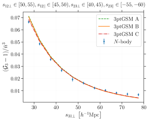
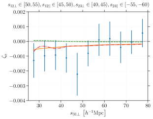
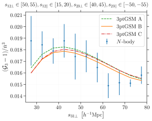
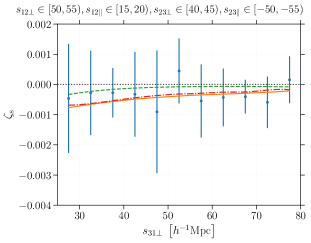
Figure 8: Left: Predictions from the 3ptGSM (lines) for the full redshift-space 3PCF $\mathcal{G}_{3}$ are compared with measurements from our $N$-body simulation (symbols with error bars). Three versions of the model are considered: case A uses as input the full 3PCF in real space $\mathcal{F}_{3}$ evaluated at LO in perturbation theory (dashed), case B also includes LO terms for $\zeta$ (solid), and case C combines the halo model for $\xi$ with the perturbative model for $\zeta$ at LO. The redshift-space separations listed on top of the figures are given in units of $h^{-1}\mathrm{Mpc}$. Right: As in the left panel, but for the connected 3PCF in redshift space.

4.3.3 Connected correlation function in real space

Feeding the 3ptGSM with an accurate input for $\zeta$ is a necessary prerequisite in order to properly test its capacity to model RSD. Therefore, in the left-panel of figure 9, we compare the real-space 3PCF obtained from the perturbative model at LO against the measurements in the simulation. We consider two narrow bins centred around $r_{12}=37.5\,h^{-1}$ Mpc and $r_{23}=62.5\,h^{-1}$ Mpc and vary $r_{31}$ within the full range. Although the agreement is not perfect, we find that the model at LO is in the same ballpark as the simulation results. Overall, the model shows the same shape dependence of the data but relative deviations range typically between 20 and 50% and, obviously, become larger around the zero-crossing points. For larger triangles with sides $r_{12}\simeq 50\,h^{-1}$ Mpc and $r_{23}\simeq 100\,h^{-1}$ Mpc, the model appears to work better (see e.g. figure 11 in [88]) but $\zeta$ becomes very small and requires large simulated volumes for an accurate measurement. All these findings are consistent with other studies on the matter 3PCF [86, 89] and bispectrum [90, 91, 92, 93, 94].

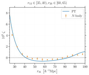
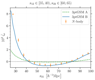
Figure 9: Left: The 3PCF in real space measured in the $N$-body simulation (symbols with error bars) is compared with the predictions from PT at LO (solid line) for a set of triangular configurations obtained by varying $r_{31}$ while keeping $r_{12}$ and $r_{23}$ fixed (as indicated by the top labels that give separations in units of $h^{-1}\mathrm{Mpc}$). Right: As in the left panel but for the spherically-averaged 3PCF in redshift space, $\bar{\zeta}_{\mathrm{s}}$. In this case, the solid line indicates the predictions of the 3ptGSM.

4.3.4 Connected correlation function averaged over all orientations

In order to compute a theoretical prediction for the spherically-averaged $\bar{\zeta}_{\mathrm{s}}$, we use equation (2.21) to evaluate $\zeta_{\mathrm{s}}$ with the 3ptGSM and calculate

$$\bar{\zeta}_{\mathrm{s}}(s_{12},s_{23},s_{31}) =\frac{\displaystyle\int\zeta_{\mathrm{s}}(\bm{s}_{12},\bm{s}_{23})\,\delta_{\mathrm{D}}^{(1)}\left(s_{31}-\sqrt{s_{12}^{2}+s_{23}^{2}+2s_{12}s_{23}\,\hat{\bm{s}}_{12}\cdot\hat{\bm{s}}_{23}}\right)\,\mathrm{d}\hat{\bm{s}}_{12}\,\mathrm{d}\hat{\bm{s}}_{23}}{\displaystyle\int\delta_{\mathrm{D}}^{(1)}\left(s_{31}-\sqrt{s_{12}^{2}+s_{23}^{2}+2s_{12}s_{23}\,\hat{\bm{s}}_{12}\cdot\hat{\bm{s}}_{23}}\right)\,\mathrm{d}\hat{\bm{s}}_{12}\,\mathrm{d}\hat{\bm{s}}_{23}}\;,$$ (4.1)

where the integrals are performed by independently varying $\hat{\bm{s}}_{12}$ and $\hat{\bm{s}}_{23}$ over the unit sphere. Note that

$$\bar{\zeta}_{\mathrm{s}}(s_{12},s_{23},s_{31}) =\frac{\displaystyle\int\zeta_{\mathrm{s}}(\bm{s}_{12},\bm{s}_{23})\,\delta_{\mathrm{D}}^{(1)}(s_{31}-\sqrt{s_{12}^{2}+s_{23}^{2}+2s_{12}s_{23}\,\hat{\bm{s}}_{12}\cdot\hat{\bm{s}}_{23}})\,\mathrm{d}\hat{\bm{s}}_{12}\,\mathrm{d}\hat{\bm{s}}_{23}}{\displaystyle 8\pi^{2}\,\int_{-1}^{+1}\delta_{\mathrm{D}}^{(1)}(s_{31}-\sqrt{s_{12}^{2}+s_{23}^{2}+2s_{12}s_{23}\,\cos\chi)}\,\mathrm{d}\cos\chi}$$

$$=\frac{\displaystyle\int\zeta_{\mathrm{s}}(\bm{s}_{12},\bm{s}_{23})\,\delta_{\mathrm{D}}^{(1)}(s_{31}-\sqrt{s_{12}^{2}+s_{23}^{2}+2s_{12}s_{23}\,\hat{\bm{s}}_{12}\cdot\hat{\bm{s}}_{23}})\,\mathrm{d}\hat{\bm{s}}_{12}\,\mathrm{d}\hat{\bm{s}}_{23}}{\displaystyle 8\pi^{2}\,\displaystyle{\frac{s_{31}}{s_{12}\,s_{23}}}\left[\Theta(s_{31}-|s_{12}-s_{23}|)-\Theta(s_{31}-s_{12}-s_{23})\right]}\;,$$ (4.2)

where $\Theta(x)$ denotes the Heaviside step function. In practice, we use the Monte Carlo method to integrate the numerator and the denominator of equation (4.1) and average over $1\,h^{-1}$ Mpc wide bins for $s_{31}$ at fixed $s_{12}$ and $s_{23}$.

In the right panel of figure 9, we plot $\bar{\zeta}_{\mathrm{s}}$ as a function of $s_{31}$ for the same triangular configurations we considered in real space. Shown are both the measurements from the simulation and the model predictions (excluding case C as it practically coincides with case B). Comparing the left and right panels reveals that RSD markedly enhance the clustering signal in the simulation, particularly for small $r_{31}$. The 3ptGSM nicely captures this trend. The agreement of our case B implementation with the simulation is rather good: the model nicely reproduces the dependence of $\bar{\zeta}_{\mathrm{s}}$ on $s_{31}$ with typical systematic deviations at the 20% level.

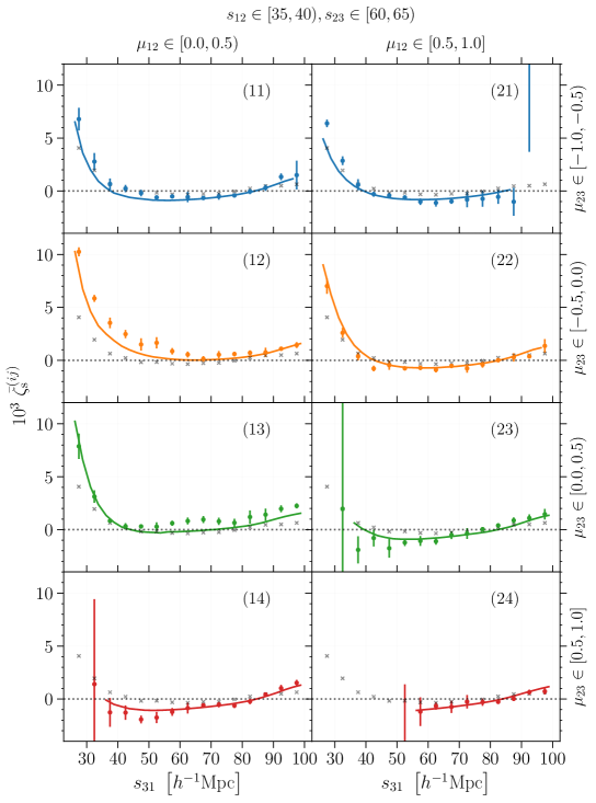
Figure 10: The wedge-averaged 3PCF measured in the simulation (symbols with error bars) is compared with the predictions of the 3ptGSM (solid lines). As a reference to help comparing the different panels, we also plot the real-space 3PCF extracted from the simulation (light $\times$ marks) and already shown in the left panel of figure 9. The side lengths of $s_{12}$ and $s_{23}$ are listed on top of the figure in units of $h^{-1}\mathrm{Mpc}$.

4.3.5 Connected correlation function averaged over wedges

Model predictions for the wedge-averaged 3PCF are obtained using equation (2.21) in combination with

$$\bar{\zeta}^{(ij)}_{\mathrm{s}}(s_{12},s_{23},s_{31}) =\frac{\displaystyle\int\zeta_{\mathrm{s}}(\bm{s}_{12},\bm{s}_{23})\,W^{(ij)}(\hat{\bm{s}}_{12}\cdot\hat{\bm{s}},\hat{\bm{s}}_{23}\cdot\hat{\bm{s}})\,\mathrm{d}\hat{\bm{s}}_{12}\,\mathrm{d}\hat{\bm{s}}_{23}}{\displaystyle\int W^{(ij)}(\hat{\bm{s}}_{12}\cdot\hat{\bm{s}},\hat{\bm{s}}_{23}\cdot\hat{\bm{s}})\,\mathrm{d}\hat{\bm{s}}_{12}\,\mathrm{d}\hat{\bm{s}}_{23}}\;,$$ (4.3)

where

$$W^{(ij)}(\mu_{12},\mu_{23})=\displaystyle\Pi_{\frac{i-1}{2},\frac{i}{2}}(\mu_{12})\,\Pi_{\frac{j-3}{2},\frac{j-2}{2}}(\mu_{23})\;,$$ (4.4)

and $\Pi_{a,b}(x)=\Theta(x-a)-\Theta(x-b)$ denotes the boxcar function. Once again we perform the integrals with the Monte Carlo method.

In figure 10, we compare the wedge-averaged correlation function $\zeta_{\mathrm{s}}^{(ij)}$ obtained from the 3ptGSM (case B) and from the simulation for the same triangular configurations considered in figure 9. The eight panels are organised as follows. The left and right columns correspond to $i=1$ (i.e. $0\leq\mu_{12}<0.5$) and $i=2$ (i.e. $0.5\leq\mu_{12}\leq 1$), respectively. Rows, from top to bottom, refer to $j=1$ ($-1\leq\mu_{23}<-0.5)$, $j=2$ ($-0.5\leq\mu_{23}<0)$, $j=3$ ($0\leq\mu_{23}<0.5)$ and $j=4$ ($0.5\leq\mu_{23}\leq 1)$. As a reference, in each panel we also show the real-space 3PCF measured in the simulation. The figure shows that RSD can enhance the 3PCF by a factor of a few (see, for instance, $\zeta_{\mathrm{s}}^{(14)}$, $\zeta_{\mathrm{s}}^{(21)}$, and $\zeta_{\mathrm{s}}^{(23)}$) as well as change its sign (as in $\zeta_{\mathrm{s}}^{(12)}$ and $\zeta_{\mathrm{s}}^{(13)}$). Independently of $s_{31}$, the 3ptGSM provides an excellent description of the numerical results for $\zeta_{\mathrm{s}}^{(24)}$, $\zeta_{\mathrm{s}}^{(23)}$ and $\zeta_{\mathrm{s}}^{(22)}$. In other cases, it works well only for large values of $s_{31}$ (see $\zeta_{\mathrm{s}}^{(21)}$, $\zeta_{\mathrm{s}}^{(11)}$, $\zeta_{\mathrm{s}}^{(12)}$ and $\zeta_{\mathrm{s}}^{(14)}$). On the other hand, the model tends to underestimate the effect of RSD for $\zeta_{\mathrm{s}}^{(13)}$ even for large opening angles.

The main conclusion emerging from the analysis of figures 8, 9, and 10 is that our implementation of the 3ptGSM, although very simple, is already able to reproduce many features measured in the simulations. This very encouraging result motivates further work into building novel tools based on the 3ptGSM for modelling $\zeta_{\mathrm{s}}$ on large scales and analyse data from galaxy redshift surveys. As a first step in this direction, in the remainder of this paper, we analyse some key aspects of the 3ptGSM and discuss how the current implementation could be improved.

4.4 Discussion

4.4.1 Dissecting the 3ptGSM

Based on equations (2.20) and (2.22), whenever $\int{\mathcal{P}}^{(3)}_{\bm{w}_{\parallel}}(w_{\parallel},q_{\parallel}|\bm{r}_{12},\bm{r}_{23})\,\mathrm{d}q_{\parallel}\neq{\mathcal{P}}^{(2)}_{w_{\parallel}}(w_{\parallel}|\bm{r}_{12})$, RSD generate a non-vanishing connected 3PCF $\zeta_{\mathrm{s}}$ even when $\zeta=0$. In the 3ptGSM, the marginalised distribution gives a Gaussian PDF with mean $m_{1}$ and variance $C_{11}$. On the other hand, ${\mathcal{P}}^{(2)}_{w_{\parallel}}$ is a Gaussian with mean $\langle w_{ij\parallel}|\bm{r}_{ij}\rangle_{\mathrm{p}}$ and variance $\langle w_{ij\parallel}^{2}|\bm{r}_{ij}\rangle_{\mathrm{p}}-\langle w_{ij\parallel}|\bm{r}_{ij}\rangle_{\mathrm{p}}^{2}$. Note that the mean values are slightly shifted and so are also the variances (although by an even smaller amount). It follows that the difference between the two PDFs does not identically vanish. In practice, however, the effect is very small. By considering, for example, the triangular configuration analysed in figure 7, we find that the mean $w_{12\parallel}$ is $-0.36$ and $-0.25$ $h^{-1}\mathrm{Mpc}$ for the marginalised ${\mathcal{P}}_{\bm{w}_{\parallel}}^{(3)}$ and for ${\mathcal{P}}_{w_{\parallel}}^{(2)}$, respectively, while the standard deviation in $\simeq 4.67\,h^{-1}\mathrm{Mpc}$ for both. It follows that the term that multiplies $1+\xi(r_{12})$ in equation (2.22) is at best of the order of $10^{-3}$ and switches sign as $w_{12}$ grows past the mean value. This is shown in figure 11 where we also plot the difference between the PDFs estimated from the simulation. The 3ptGSM provides a reasonable approximation to the numerical results. The total contribution of terms like this one to $\zeta_{\mathrm{s}}$ is shown in the right panels of figures 8 and 9 as the result of our case A model. Note that it is always subdominant with respect to the contribution generated by $\zeta$, at least for the configurations considered here. There is some evidence that the terms proportional to $1+\xi$ in equation (2.22) might become more relevant at small scales where the mean relative velocities are not so small compared to the dispersion. For instance, they appear to give a $\sim 25\%$ contribution to $\bar{\zeta}_{\mathrm{s}}$ for the smallest values of $s_{31}$ shown in figure 9. However, it is unclear whether such small scales can be robustly analysed with the 3ptGSM.

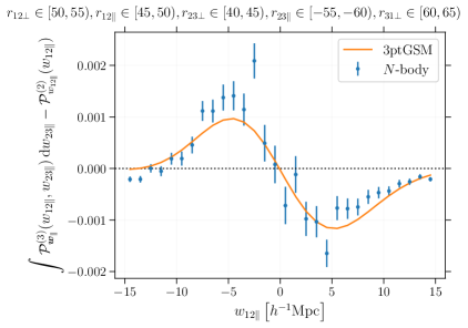
Figure 11: The difference of probability densities appearing in the rhs of equation (2.22). Symbols with error bars represent measurements from the $N$-body simulation while the dashed line shows the predictions of the 3ptGSM.

In figure 12, we plot the different terms that appear in the rhs of equation (2.20) using the same triangular configurations as in figure 8. The first thing to notice is that $\zeta_{\mathrm{s}}$ is obtained by subtracting two much larger numbers. This evidences the need for modelling $\mathcal{P}_{w_{\parallel}}^{(2)}$ and $\mathcal{P}_{\bm{w}_{\parallel}}^{(3)}$ in a consistent way. Also note that the integral $\int\mathcal{P}_{\bm{w}_{\parallel}}^{(3)}\,\mathrm{d}w_{\parallel}\,\mathrm{d}q_{\parallel}$ appearing in the last row of equation (2.20) is not identically equal to one as the conditional PDF needs to be evaluated considering different triangular configurations that reflect the running of the real-space parallel separations in the integral.

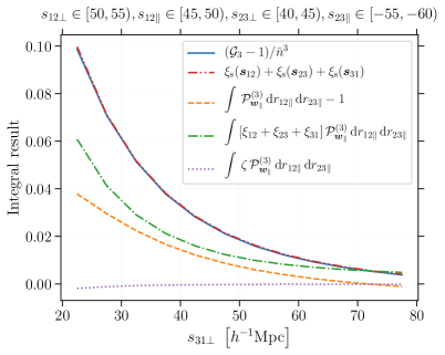
Figure 12: Partial contributions to the rhs of equation (2.21) in the 3ptGSM for the same triangular configurations displayed in the top row of figure 8 (particle separations are given on top of the figure in units of $h^{-1}\mathrm{Mpc}$). The solid curve represents the integral containing the full 3PCF in real space. The dash double dotted line (hardly distinguishable from the solid one) displays the sum of the three integrals containing the two-point correlation function. The connected 3PCF in redshift space is derived by subtracting the second contribution from the first. Note that the value of $\zeta_{\mathrm{s}}$ is a small number obtained by subtracting two much larger numbers. The dashed, dash-dotted and dotted lines isolate the three sub-components of the solid curve. Namely, they show the part proportional to 1, $\xi$ and $\zeta$, respectively.

Although the Gaussian approximation for ${\mathcal{P}}^{(2)}_{w_{\parallel}}$ is not perfect, the Gaussian streaming model provides a very good description of $\xi_{\mathrm{s}}$ on large scales [e.g. 7]. This success originates from fortuitous cancellations between the contributions of the peak and the wings in the integrand of equation (2.14) (see figure 4 in [19]). In figure 13, we show that the same phenomenon takes place in the 3ptGSM. Shown with solid lines are contour levels of the integrand appearing in the rhs of equation (2.21) for a configuration in which the 3ptGSM accurately reproduces the full 3PCF measured in the simulation. We extract the same quantity from the simulation by creating a bivariate histogram of $s_{ij\parallel}-w_{ij\parallel}$ for the particle triplets that form the same triangular configuration and making sure that its integral gives ${\mathcal{G}}_{3}$. The corresponding contour levels are plotted with dashed lines. From the figure, it is evident that the peak of the integrand in the 3ptGSM is underestimated and the tails are overestimated when compared to the numerical results. This provides motivation for improving the modelling of ${\mathcal{P}}^{(3)}_{\bm{w}_{\parallel}}$ along the lines that have been already used for the 2PCF [e.g. 16, 17, 18, 19, 20].

An even more direct consistency test of the 3ptGSM can be performed by measuring the real-space correlations and velocity moments from the simulation and inserting them into the key equations of the model to isolate the impact of the Gaussian assumption, as it has been done for 2-point statstics [19]. However, this investigation would be very time consuming as it requires accurate measurements for all possible triangular configurations up to (at least) $r\sim 150\ h^{-1}\ \mathrm{Mpc}$ (for the range of separations considered in this work). For this reason, we postpone this study to future work.

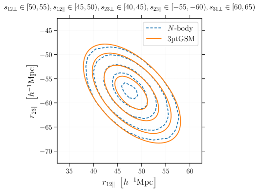
Figure 13: Contour levels of the integrand appearing in the rhs of equation (2.19) for one of the triangular configuration shown in figures 8 and 12 (particle separations are given on top of the figure in units of $h^{-1}\mathrm{Mpc}$). Solid and dashed lines correspond to the 3ptGSM and the $N$-body simulation, respectively. Contours correspond to the levels $\{8,6,4,2,1\}\times 10^{-3}$ with the values decreasing from inside to outside. Note that the predictions of the GSM do not reach the value $8\times 10^{-3}$.

4.4.2 Directions for future improvements

Overall, the simple version of the 3ptGSM we have implemented captures the main trends that can be observed in the simulation. However, there are some discrepancies. We identify a number of reasons for this partial agreement. First of all, the model we use for $\zeta$ needs to be substantially improved. As discussed above (left panel of figure 9) perturbation theory at LO only provides a sketchy description of the simulation data for the corresponding triangular configuration in real space (i.e. using $r_{12}=s_{12}$ and $r_{23}=s_{23}$). However, the situation is worse than that. In fact, the integral that gives $\zeta_{\mathrm{s}}(\triangle_{123})$ in the streaming model receives contributions from triangles with pairwise separations $r_{ij\parallel}$ and $r_{ij\perp}$ that differ by up to 40-50 $h^{-1}$ Mpc from those that define $\triangle_{123}$. For some of them, the model for $\zeta$ at LO does not perform very well. Moreover, the second moments of the pairwise velocities predicted with standard perturbation theory at LO become progressively less accurate for squeezed triangles. One can notice this trend in some capacity already in the rightmost panels of figure 5 and in the top-right panel of figure 6: the model increasingly departs from the simulation results as $r_{31}$ and $r_{31\perp}$ decrease. Since the double integral in equation (2.21) runs over all sorts of triangular configurations including some squeezed ones, this generates inaccuracies. As we have seen in section 4.4, the 3ptGSM prediction for $\zeta_{\mathrm{s}}$, which is of the order of $\xi^{2}$, is obtained from the subtraction of two much larger numbers of order $\xi$ (this can also be noticed by comparing the left and right panels in figure 8). Therefore, relatively small errors in the terms that need to be subtracted can shift $\zeta_{\mathrm{s}}$ substantially. We thus expect that the 3ptGSM will considerably benefit from more sophisticated input models for $\xi$, $\zeta$ and the moments of the pairwise velocities as it has already happened at the 2-point level [8, 78, 10]. Implementing these improvements, however, clearly goes beyond the scope of this paper.

4.4.3 Connection with dispersion models for the bispectrum

Fourier transforming equation (2.14) provides an expression for the anisotropic power spectrum in redshift space, $P_{\mathrm{s}}(k_{\parallel},k_{\perp})$. If one is ready to assume, for simplicity, that ${\mathcal{P}}^{(2)}_{w_{\parallel}}(w_{\parallel}|\bm{r})$ does not depend on $\bm{r}$, the convolution theorem then gives $P_{\mathrm{s}}(k_{\parallel},k_{\perp})=S^{(2)}(k_{\parallel})\,P(k_{\parallel},k_{\perp})$ with $S^{(2)}(k_{\parallel})$ the Fourier transform of ${\mathcal{P}}^{(2)}_{w_{\parallel}}$. This situation occurs if ${\mathcal{P}}^{(2)}_{w_{\parallel}}(w_{\parallel}|\bm{r})$ is replaced by the scale-independent function ${\mathcal{R}}_{w_{\parallel}}^{(2)}(w_{\parallel})$ we have introduced in equation (2.29). This defines the so-called ‘dispersion model’. The basic underlying idea (originally proposed in [95]) is to imagine that, due to highly non-linear physics taking place on small scales, the los velocity at each spatial location has a random component which is independently drawn from a distribution with variance $\sigma^{2}_{v}$ and the los relative velocities between two locations have thus a variance of $\sigma^{2}_{\rm p}=2\,\sigma^{2}_{v}$. Assuming that ${\mathcal{P}}^{(1)}_{v_{\parallel}}$ is well approximated by a zero-mean Gaussian with variance $\sigma^{2}_{{v}}$ gives $S^{(2)}(k_{\parallel})=\exp(-k_{\parallel}^{2}\,\sigma_{\mathrm{p}}^{2}/2)$ which reduces to $S^{(2)}(k_{\parallel})\simeq 1-k_{\parallel}^{2}\,\sigma_{\mathrm{p}}^{2}/2$ on large scales. This expression is commonly used to analyse survey and simulation data [e.g. 96, 97, 98, 99, 100, 101, 102] and $\sigma^{2}_{\mathrm{p}}$ is treated as a free parameter. The ‘damping factor’ $S^{(2)}(k_{\parallel})$ thus accounts for the suppression of the clustering amplitude in redshift space due to incoherent relative motions along the los generated within collapsed structures (e.g. the ‘finger-of-god’ effect [1, 2]).

We now use equation (2.21) to generalise the dispersion model to 3-point statistics. The 3PCF and the bispectrum $B(\bm{p},\bm{q},\bm{k})$ form a Fourier pair, i.e.

$$\zeta(\triangle_{123}) =\langle\delta(\bm{x}_{2})\,\delta(\bm{x}_{2}+\bm{r}_{21})\,\delta(\bm{x}_{2}+\bm{r}_{23})\rangle$$

$$=\int B(\bm{p},\bm{q},-\bm{p}-\bm{q})\,e^{-i\left(\bm{p}\cdot\bm{r}_{21}+\bm{q}\cdot\bm{r}_{23}\right)}\,\frac{\mathrm{d}^{3}p\,\mathrm{d}^{3}q}{(2\pi)^{6}}\;,$$ (4.5)

(note that the correlation function is defined in terms of the ‘star ray’ separation $\bm{r}_{21}$ introduced in footnote 2 while we have always used $\bm{r}_{12}$ so far). Let us now consider the simplest possible case in which: (i) $\mathcal{P}_{\bm{w}_{\parallel}}^{(3)}$ does not depend on $\bm{r}_{21}$ and $\bm{r}_{23}$, (ii) the PDF of the pairwise velocities can be approximated by a Gaussian distribution with covariance matrix ${\bm{\mathsf{\Sigma}}}$, and (iii) the contribution from the two-point terms in the rhs of equation (2.20) is subdominant (as discussed above). In this case, the convolution theorem gives

$$B_{\mathrm{s}}(\bm{p},\bm{q},-\bm{p}-\bm{q})=S^{(3)}(p_{\parallel},q_{\parallel})\,B(\bm{p},\bm{q},-\bm{p}-\bm{q})\;,$$ (4.6)

with

$$S^{(3)}(p_{\parallel},q_{\parallel}) =\int{\mathcal{P}}^{(3)}_{\bm{w}_{\parallel}}(w_{21\parallel},w_{23\parallel}|\triangle_{123})\,e^{i(p_{\parallel}w_{21\parallel}+q_{\parallel}w_{23\parallel})}\,\mathrm{d}w_{21\parallel}\,\mathrm{d}w_{23\parallel}$$

$$=\exp\left[-\frac{1}{2}(\Sigma_{11}\,p_{\parallel}^{2}+2\,\Sigma_{12}\,p_{\parallel}\,q_{\parallel}+\Sigma_{22}\,q_{\parallel}^{2})\right]\;.$$ (4.7)

However, the result must be invariant with respect to changing the pair of wavevectors we use to evaluate the damping factor, i.e. $S^{(3)}(p_{\parallel},q_{\parallel})=S^{(3)}(p_{\parallel},-p_{\parallel}-q_{\parallel})=S^{(3)}(-p_{\parallel}-q_{\parallel},q_{\parallel})$. It follows that the covariance matrix must have the form

$${\bm{\mathsf{\Sigma}}}=\sigma^{2}\begin{pmatrix}1&1/2\\ 1/2&1\end{pmatrix}\;,$$ (4.8)

with $\sigma^{2}$ a free parameter. For convenience, in this calculation we have used the variable $w_{21\parallel}$ while in the remainder of the paper we always dealt with $w_{12\parallel}=-w_{21\parallel}$. Therefore, equation (4.8) can be re-written in terms of the covariance matrix ${\bm{\mathsf{C}}}$ we have introduced in section 4.1 as

$${\bm{\mathsf{C}}}=\sigma^{2}\begin{pmatrix}1&-1/2\\ -1/2&1\end{pmatrix}\;.$$ (4.9)

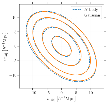
Figure 14: Contour levels of the scale-independent PDF $\mathcal{R}^{(3)}_{\bm{w}_{\parallel}}$, as given in equation (2.37). The dashed lines correspond to the direct measurement from the simulation while the solid lines represent a zero mean bivariate Gaussian with a covariance matrix of the same form as in equation (4.9) and $\sigma^{2}=24.2\ h^{-2}\mathrm{Mpc}^{2}$. Contours correspond to levels $\{6,3,1,0.4\}\times 10^{-3}$ with the values decreasing from inside to outside.

It is reassuring to see that this result provides a zeroth-order approximation to the velocity statistics we measure in the $N$-body simulation as shown in the bottom-right panel of figure 1 and in figure 6. On large scales, the mean pairwise velocities are much smaller than their dispersions which are nearly scale independent. Moreover, the linear correlation coefficient between $w_{12\parallel}$ and $w_{23\parallel}$ is always close to $-1/2$.

Equation (4.9) has a simple and straightforward interpretation within the context of the dispersion model: if the los velocity at each location is independently drawn from a distribution with variance $\sigma^{2}_{v}$, then ${\bm{\mathsf{C}}}$ is the covariance matrix of the velocity differences $w_{12\parallel}$ and $w_{23\parallel}$. The non-vanishing off-diagonal term comes from the fact that location number 2 appears in both pairs as evidenced in equation (3.25). Therefore, we can write that $\sigma^{2}=\sigma^{2}_{\mathrm{p}}=2\,\sigma^{2}_{v}$. In other words, in full analogy with the 2-point case, the dispersion model is obtained by replacing ${\mathcal{P}}^{(3)}_{\bm{w}_{\parallel}}$ with the function ${\mathcal{R}}^{(3)}_{\bm{w}_{\parallel}}$ introduced in equation (2.37). While completing this work, we became aware that this line of reasoning was first pursued in reference [103] to model the galaxy 3PCF on small scales. This publication also introduces a very rudimentary form of our equation (2.17) in which ${\mathcal{R}}^{(3)}_{\bm{w}_{\parallel}}$ appears instead of ${\mathcal{P}}^{(3)}_{\bm{w}_{\parallel}}$. In figure 14, we show that a Gaussian PDF provides an excellent approximation to ${\mathcal{R}}^{(3)}_{\bm{w}_{\parallel}}$.

In the literature on the bispectrum, the damping factor is generally written as a symmetric function of three wavenumbers, ${\mathcal{F}}(p_{\parallel},q_{\parallel},k_{\parallel})$ with the condition $p_{\parallel}+q_{\parallel}+k_{\parallel}=0$. Equations (4.7) and (4.9) say that ${\mathcal{F}}(p_{\parallel},q_{\parallel},-p_{\parallel}-q_{\parallel})=S^{(3)}(p_{\parallel},q_{\parallel})$. There are multiple functional forms for ${\mathcal{F}}$ that satisfy this condition. For instance, we could obtain a valid ${\mathcal{F}}$ by applying a symmetrization method either to the function $S^{(3)}$ (i.e. ${\mathcal{F}}(p_{\parallel},q_{\parallel},k_{\parallel})=[S^{(3)}(p_{\parallel},q_{\parallel})+S^{(3)}(p_{\parallel},k_{\parallel})+S^{(3)}(k_{\parallel},q_{\parallel})]/3$) or to the argument of the exponential function that appears in $S^{(3)}$ (i.e. ${\mathcal{F}}(p_{\parallel},q_{\parallel},k_{\parallel})=\exp[-(2p_{\parallel}^{2}+2q_{\parallel}^{2}+2k_{\parallel}^{2}+pq+kp+kq)\sigma^{2}/6]$). A simpler solution is found by further requiring that $\mathcal{F}$ only depends on the square of the wavenumbers which gives ${\mathcal{F}}(p_{\parallel},q_{\parallel},k_{\parallel})=\exp[-(p_{\parallel}^{2}+q_{\parallel}^{2}+k_{\parallel}^{2})\,\sigma^{2}_{\mathrm{p}}/4]\simeq 1-(p_{\parallel}^{2}+q_{\parallel}^{2}+k_{\parallel}^{2})\,\sigma^{2}_{\mathrm{p}}/4$. In brief, providing an expression for ${\mathcal{F}}$ is somewhat arbitrary. All what matters in practice is the function $S^{(3)}$.

4.4.4 Dependence on the growth rate of structure

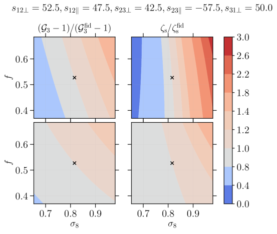
Figure 15: Dependence of ${\mathcal{G}}_{3}$ and $\zeta_{\mathrm{s}}$ on $f$ and $\sigma_{8}$ in the 3ptGSM. Shown are the contour levels of the ratios $({\mathcal{G}}_{3}-1)/({\mathcal{G}}^{\mathrm{fid}}_{3}-1)$ (left) and $\zeta_{\mathrm{s}}/\zeta_{\mathrm{s}}^{\mathrm{fid}}$ (right) where the fiducial values for $f$ and $\sigma_{8}$ coincide with those used in our simulation and are highlighted by the crosses. The top panels represent the full dependence of the 3PCFs while the bottom ones do not consider the overall normalisation of the real-space functions $\xi$ and $\zeta$ (which would be degenerate with the linear bias factor in actual survey data). The separations that define the triangular configuration are indicated on top of the figure in units of $h^{-1}\mathrm{Mpc}$.

Measurements of the linear growth rate of structure $f(z)$ through RSDs are used to probe gravity and the nature of dark energy [105, 106]. This is one of the main drivers for developing the next generation of galaxy redshift surveys. Although the implementation of the 3ptGSM discussed in this paper applies to the clustering of matter and extensions to biased tracers will be needed for direct applications to survey science, it is anyway interesting to provide a few illustrative examples of how the 3ptGSM responds to variations in the growth rate of structure.

In the top panels of figure 15, we show the dependence of ${\mathcal{G}}_{3}$ and $\zeta_{\mathrm{s}}$ on $f$ and $\sigma_{8}$ for a particular triangle configuration. All the other parameters that determine the linear power spectrum are kept unchanged. The shape of the contours is determined by the dependencies of the different ingredients of the streaming model: the mean pairwise velocity in equation (3.5) scales as $f\sigma_{8}^{2}$, the velocity dispersion in equations (3.20) and (3.21) as $(f\sigma_{8})^{2}$, and the leading-order perturbative terms for $\xi$ and $\zeta$ as $\sigma_{8}^{2}$ and $\sigma_{8}^{4}$, respectively. In the bottom panels, we scale out the normalisation of the real-space statistics in order to focus on the effects of the RSD. It is worth noticing that $\zeta_{\mathrm{s}}$ and ${\mathcal{G}}_{3}$ (which is dominated by 2-point statistics) display different degeneracies in the $f$-$\sigma_{8}$ plane. Since RSD in the galaxy power spectrum on large scales are only sensitive to the degenerate combination $f\sigma_{8}$ and $b\sigma_{8}$ (where $b$ denotes the linear bias parameter), the results above suggest that measuring $\zeta_{\mathrm{s}}$ with sufficient accuracy should be able to break the $f$-$\sigma_{8}$ degeneracy (see also [107] for a related conclusion based on Fourier-space statistics). In figure 16, we show the dependence of $\zeta_{\mathrm{s}}$ and $\bar{\zeta}_{\mathrm{s}}$ on $f$ while keeping $\sigma_{8}$ fixed at its fiducial value (for some of the configurations displayed in figures 8 and 9). Thirty per cent variations in $f$ induce scale-dependent changes in $\zeta_{\mathrm{s}}$ at the 10-20% level and modulate the amplitude of $\bar{\zeta}_{\mathrm{s}}$ by 7-12%. On large scales (and for bins that are similar to ours), the Euclid mission is expected to measure $\bar{\zeta}_{\mathrm{s}}$ with an accuracy of $\sim$10% on the individual data points (A. Veropalumbo, private communication). Slightly larger uncertainties should be expected for the wedge-averaged 3PCF while measurements of $\zeta_{\mathrm{s}}$ should suffer from a substantially lower signal-to-noise ratio. Considering the large number of possible triangular configurations, our results suggest that the 3PCF should be able to provide a competitive measurement of the growth rate of structure. Performing an accurate forecast, however, requires an estimation of the covariance matrix of the measurements and goes clearly beyond the scope of this paper.

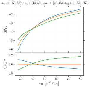
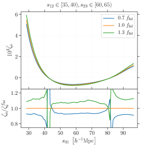
Figure 16: Variations of $\zeta_{\mathrm{s}}$ (left) and $\bar{\zeta}_{\mathrm{s}}$ (right) with $f$ in the 3ptGSM for some of the triangular configurations shown in figures 8 and 9.

5 Summary

We have derived, from first principles, the equations that relate the $n$-point correlation functions in real and redshift space. We have followed a particle-based approach using statistical-mechanics techniques based on the $n$-particle phase-space densities. Our results are exact (within the distant-observer approximation) and completely independent of the nature of the tracers we consider and of their interactions. They generalise the so-called streaming model to $n$-point statistics. The theory is formulated more naturally in terms of the full $n$-point correlations. In this case, the redshift-space correlation function is obtained as an integral of its real-space counterpart times the joint PDF of $n-1$ relative los peculiar velocities. Equation (2.17) expresses this relation succinctly and the velocity PDF is defined in equation (2.16).

We have shown that it is possible to re-formulate the theory entirely in terms of connected correlation functions although the price to pay is a velocity term that is not a PDF (and can be negative) as well as a higher degree of abstractness. This result is expressed by equations (2.31) and (2.32).

In the second part of the paper, we have focused on 3-point statistics. First of all, by combining the streaming model for the 2PCF and the 3PCF, we have derived equation (2.21) which provides a computationally-friendly framework to calculate connected 3-point correlations in redshift space. A key ingredient appearing in this equation is the bivariate PDF for the los relative velocities between particles pairs in a triplet, ${\mathcal{P}}^{(3)}_{\bm{w}_{\parallel}}(w_{12\parallel},w_{23\parallel}|\triangle_{123})$. Making use of a large $N$-body simulation, we have characterised the properties of this function for unbiased tracers of the matter-density field. Figures 1 and 7 show that the PDF is unimodal and, for large triangles, has a quasi-Gaussian peak. The dispersion of $w_{12\parallel}$ and $w_{23\parallel}$ is always much larger than the mean. Moreover, $w_{12\parallel}$ and $w_{23\parallel}$ tend to be anti-correlated, especially on large scales.

In section 3.3, we have derived theoretical predictions for the first two moments of $\bm{w}_{12}$ and $\bm{w}_{23}$ using standard perturbation theory at LO. Equation (3.6) shows that the mean relative velocity between a particle pair in a triplet is not purely radial but has also a transverse component in the plane of the triangle defined by the particles. Individual expressions for the different components are given in equations (3.7), (3.8) and (3.9). Figures 3 and 4 show that the LO predictions accurately match the simulation results from quasi-linear scales onward ($r_{ij}\gtrsim 20\,h^{-1}\mathrm{Mpc}$). Perturbative expressions for the second moments are given in equations (3.26) and (3.27). In this case, a constant offset needs to be added to the theoretical results (that neglect small-scale physics) in order to reproduce the simulations on large scales. Figure 5 shows that, after applying the correction, the model is accurate to better than a few per cent for separations $r_{ij}\gtrsim 50\,h^{-1}\mathrm{Mpc}$. In section 3.3.3, we have discussed the projection of the relative velocities along the los. Figure 6 shows that the perturbative predictions agree well with the simulation for triangles with legs $r_{ij}\gtrsim 50\,h^{-1}\mathrm{Mpc}$. Our results lay the groundwork for investigating 3-point statistics of the los pairwise velocities with future experiments based on the kinetic Sunyaev-Zel’dovich effect like the Simons Observatory [SO, 108], CMB-S4 [109], CMB-HD [110, 111]; as well as with other peculiar-velocity surveys like the Taipan galaxy survey [Taipan, 112] and the Widefield ASKAP L-band Legacy All-sky Blind Survey [WALLABY, 113].

In section 4, we have introduced the 3ptGSM that brings together several elements of our study. This model is based on the exact equation (2.21) but phenomenologically approximates ${\mathcal{P}}^{(3)}_{\bm{w}_{\parallel}}(w_{12\parallel},w_{23\parallel}|\triangle_{123})$ with a bivariate Gaussian distribution whose moments are computed using perturbative techniques (and offsetting the velocity dispersion with a constant so that to match its direct measurement in the simulation). We have then presented a simple practical implementation of the 3ptGSM by deriving all its ingredients (real-space clustering amplitudes and velocity statistics) from standard perturbation theory at LO. The comparison of the model predictions against the correlation function from the simulation performed in figures 8, 9 and 10 is very encouraging, in particular considering that the model has no free parameters.

The forthcoming generation of galaxy surveys will cover large-enough volumes to permit accurate measurements of the 3PCF on large scales. This achievement will inform us about galaxy formation, cosmology, neutrino masses, the nature of primordial perturbations, dark energy, and the gravity law. It is thus timely to create new theoretical tools that facilitate this endeavour. In this paper, we have developed a general framework for the analysis of RSDs in the $n$-point correlation functions. This pilot work sets the foundation for future developments including: (i) considering biased tracers of the matter-density field, (ii) extending our calculations to different flavours of PT [e.g. 7, 8, 10] for both real-space clustering and velocity statistics, and (iii) going beyond the Gaussian approximation for the PDF of the relative los velocities by introducing multivariate distributions with non-zero skewness and that are leptokurtic [e.g. 16, 17, 18, 19, 20].

References

- [1] J. C. Jackson, A critique of Rees’s theory of primordial gravitational radiation, Mon. Not. R. Astron. Soc. 156 (1972) 1P, [0810.3908].
- [2] W. L. W. Sargent and E. L. Turner, A statistical method for determining the cosmological density parameter from the redshifts of a complete sample of galaxies, Astrophys. J. Lett 212 (Feb., 1977) L3–L7.
- [3] N. Kaiser, Clustering in real space and in redshift space, Mon. Not. R. Astron. Soc. 227 (July, 1987) 1–21.
- [4] A. J. S. Hamilton, Linear Redshift Distortions: a Review, in The Evolving Universe (D. Hamilton, ed.), vol. 231 of Astrophysics and Space Science Library, p. 185, 1998, astro-ph/9708102, DOI.
- [5] P. J. E. Peebles, The large-scale structure of the universe. Princeton Series in Physics. Princeton University Press, 1980.
- [6] K. B. Fisher, On the Validity of the Streaming Model for the Redshift-Space Correlation Function in the Linear Regime, Astrophys. J. 448 (Aug., 1995) 494, [astro-ph/9412081].
- [7] B. A. Reid and M. White, Towards an accurate model of the redshift-space clustering of haloes in the quasi-linear regime, Mon. Not. R. Astron. Soc. 417 (Nov., 2011) 1913–1927, [1105.4165].
- [8] J. Carlson, B. Reid and M. White, Convolution Lagrangian perturbation theory for biased tracers, Mon. Not. R. Astron. Soc. 429 (Feb., 2013) 1674–1685, [1209.0780].
- [9] M. White, B. Reid, C.-H. Chuang, J. L. Tinker, C. K. McBride, F. Prada et al., Tests of redshift-space distortions models in configuration space for the analysis of the BOSS final data release, Mon. Not. R. Astron. Soc. 447 (Feb., 2015) 234–245, [1408.5435].
- [10] Z. Vlah, E. Castorina and M. White, The Gaussian streaming model and convolution Lagrangian effective field theory, J. Cosmol. Astropart. Phys. 12 (Dec., 2016) 007, [1609.02908].
- [11] B. A. Reid, L. Samushia, M. White, W. J. Percival, M. Manera, N. Padmanabhan et al., The clustering of galaxies in the SDSS-III Baryon Oscillation Spectroscopic Survey: measurements of the growth of structure and expansion rate at z = 0.57 from anisotropic clustering, Mon. Not. R. Astron. Soc. 426 (Nov., 2012) 2719–2737, [1203.6641].
- [12] L. Samushia, B. A. Reid, M. White, W. J. Percival, A. J. Cuesta, G.-B. Zhao et al., The clustering of galaxies in the SDSS-III Baryon Oscillation Spectroscopic Survey: measuring growth rate and geometry with anisotropic clustering, Mon. Not. R. Astron. Soc. 439 (Apr., 2014) 3504–3519, [1312.4899].
- [13] S. Alam, S. Ho, M. Vargas-Magaña and D. P. Schneider, Testing general relativity with growth rate measurement from Sloan Digital Sky Survey - III. Baryon Oscillations Spectroscopic Survey galaxies, Mon. Not. R. Astron. Soc. 453 (Oct., 2015) 1754–1767, [1504.02100].
- [14] C.-H. Chuang, M. Pellejero-Ibanez, S. Rodríguez-Torres, A. J. Ross, G.-b. Zhao, Y. Wang et al., The clustering of galaxies in the completed SDSS-III Baryon Oscillation Spectroscopic Survey: single-probe measurements from DR12 galaxy clustering - towards an accurate model, Mon. Not. R. Astron. Soc. 471 (Oct., 2017) 2370–2390, [1607.03151].
- [15] S. Satpathy, S. Alam, S. Ho, M. White, N. A. Bahcall, F. Beutler et al., The clustering of galaxies in the completed SDSS-III Baryon Oscillation Spectroscopic Survey: on the measurement of growth rate using galaxy correlation functions, Mon. Not. R. Astron. Soc. 469 (Aug., 2017) 1369–1382, [1607.03148].
- [16] D. Bianchi, M. Chiesa and L. Guzzo, Improving the modelling of redshift-space distortions - I. A bivariate Gaussian description for the galaxy pairwise velocity distributions, Mon. Not. R. Astron. Soc. 446 (Jan., 2015) 75–84, [1407.4753].
- [17] C. Uhlemann, M. Kopp and T. Haugg, Edgeworth streaming model for redshift space distortions, Phys. Rev. D. 92 (Sept., 2015) 063004, [1503.08837].
- [18] D. Bianchi, W. J. Percival and J. Bel, Improving the modelling of redshift-space distortions- II. A pairwise velocity model covering large and small scales, Mon. Not. R. Astron. Soc. 463 (Dec., 2016) 3783–3798, [1602.02780].
- [19] J. Kuruvilla and C. Porciani, On the streaming model for redshift-space distortions, Mon. Not. R. Astron. Soc. (June, 2018) , [1710.09379].
- [20] C. Cuesta-Lazaro, B. Li, A. Eggemeier, P. Zarrouk, C. M. Baugh, T. Nishimichi et al., Towards a non-Gaussian model of redshift space distortions, arXiv e-prints (Feb., 2020) , [2002.02683].
- [21] P. J. E. Peebles and E. J. Groth, Statistical analysis of catalogs of extragalactic objects. V - Three-point correlation function for the galaxy distribution in the Zwicky catalog, Astrophys. J. 196 (Feb., 1975) 1–11.
- [22] E. J. Groth and P. J. E. Peebles, Statistical analysis of catalogs of extragalactic objects. VII - Two- and three-point correlation functions for the high-resolution Shane-Wirtanen catalog of galaxies, Astrophys. J. 217 (Oct., 1977) 385–405.
- [23] P. J. E. Peebles, The mass of the universe, Annals of the New York Academy of Sciences 375 (Dec, 1981) 157–168.
- [24] A. J. Bean, R. S. Ellis, T. Shanks, G. Efstathiou and B. A. Peterson, A complete galaxy redshift sample. I - The peculiar velocities between galaxy pairs and the mean mass density of the Universe, Mon. Not. R. Astron. Soc. 205 (Nov., 1983) 605–624.
- [25] G. Efstathiou and R. I. Jedrzejewski, Observational constraints on dark matter in the universe, Advances in Space Research 3 (Jan, 1984) 379–386.
- [26] D. Hale-Sutton, R. Fong, N. Metcalfe and T. Shanks, An extended galaxy redshift survey. II - Virial constraints on . III - Constraints on large-scale structure, Mon. Not. R. Astron. Soc. 237 (Apr., 1989) 569–587.
- [27] Y. P. Jing and G. Börner, The Three-Point Correlation Function of Galaxies Determined from the Las Campanas Redshift Survey, Astrophys. J. 503 (Aug., 1998) 37–47, [astro-ph/9802011].
- [28] Y. P. Jing and G. Börner, The Three-Point Correlation Function of Galaxies Determined from the Two-Degree Field Galaxy Redshift Survey, Astrophys. J. 607 (May, 2004) 140–163, [astro-ph/0311585].
- [29] Y. Wang, X. Yang, H. J. Mo, F. C. van den Bosch and Y. Chu, The three-point correlation function of galaxies: comparing halo occupation models with observations, Mon. Not. R. Astron. Soc. 353 (Sept., 2004) 287–300, [astro-ph/0404143].
- [30] E. Gaztañaga, P. Norberg, C. M. Baugh and D. J. Croton, Statistical analysis of galaxy surveys - II. The three-point galaxy correlation function measured from the 2dFGRS, Mon. Not. R. Astron. Soc. 364 (Dec., 2005) 620–634, [astro-ph/0506249].
- [31] I. Kayo, Y. Suto, R. C. Nichol, J. Pan, I. Szapudi, A. J. Connolly et al., Three-Point Correlation Functions of SDSS Galaxies in Redshift Space: Morphology, Color, and Luminosity Dependence, Publ. Astron. Soc. Jap. 56 (June, 2004) 415–423, [astro-ph/0403638].
- [32] R. C. Nichol, R. K. Sheth, Y. Suto, A. J. Gray, I. Kayo, R. H. Wechsler et al., The effect of large-scale structure on the SDSS galaxy three-point correlation function, Mon. Not. R. Astron. Soc. 368 (June, 2006) 1507–1514, [astro-ph/0602548].
- [33] A. J. Ross, R. J. Brunner and A. D. Myers, Precision Measurements of Higher Order Angular Galaxy Correlations Using 11 Million SDSS Galaxies, Astrophys. J. 649 (Sep, 2006) 48–62, [astro-ph/0605748].
- [34] G. V. Kulkarni, R. C. Nichol, R. K. Sheth, H.-J. Seo, D. J. Eisenstein and A. Gray, The three-point correlation function of luminous red galaxies in the Sloan Digital Sky Survey, Mon. Not. R. Astron. Soc. 378 (July, 2007) 1196–1206, [astro-ph/0703340].
- [35] E. Gaztañaga, A. Cabré, F. Castander, M. Crocce and P. Fosalba, Clustering of luminous red galaxies - III. Baryon acoustic peak in the three-point correlation, Mon. Not. R. Astron. Soc. 399 (Oct., 2009) 801–811, [0807.2448].
- [36] C. K. McBride, A. J. Connolly, J. P. Gardner, R. Scranton, J. A. Newman, R. Scoccimarro et al., Three-point Correlation Functions of SDSS Galaxies: Luminosity and Color Dependence in Redshift and Projected Space, Astrophys. J. 726 (Jan., 2011) 13, [1007.2414].
- [37] F. Marín, The Large-scale Three-point Correlation Function of Sloan Digital Sky Survey Luminous Red Galaxies, Astrophys. J. 737 (Aug., 2011) 97, [1011.4530].
- [38] H. Guo, C. Li, Y. P. Jing and G. Börner, Stellar Mass and Color Dependence of the Three-point Correlation Function of Galaxies in the Local Universe, Astrophys. J. 780 (Jan., 2014) 139, [1303.2609].
- [39] H. Guo, Z. Zheng, Y. P. Jing, I. Zehavi, C. Li, D. H. Weinberg et al., Modelling the redshift-space three-point correlation function in SDSS-III, Mon. Not. R. Astron. Soc. 449 (Apr., 2015) L95–L99, [1409.7389].
- [40] Z. Slepian, D. J. Eisenstein, F. Beutler, C.-H. Chuang, A. J. Cuesta, J. Ge et al., The large-scale three-point correlation function of the SDSS BOSS DR12 CMASS galaxies, Mon. Not. R. Astron. Soc. 468 (June, 2017) 1070–1083.
- [41] F. A. Marín, C. Blake, G. B. Poole, C. K. McBride, S. Brough, M. Colless et al., The WiggleZ Dark Energy Survey: constraining galaxy bias and cosmic growth with three-point correlation functions, Mon. Not. R. Astron. Soc. 432 (July, 2013) 2654–2668, [1303.6644].
- [42] M. Moresco, F. Marulli, L. Moscardini, E. Branchini, A. Cappi, I. Davidzon et al., The VIMOS Public Extragalactic Redshift Survey (VIPERS) . Exploring the dependence of the three-point correlation function on stellar mass and luminosity at 0.5 < < 1.1, Astron. Astrophys. 604 (Aug, 2017) A133, [1603.08924].
- [43] M. Levi, C. Bebek, T. Beers, R. Blum, R. Cahn, D. Eisenstein et al., The DESI Experiment, a whitepaper for Snowmass 2013, ArXiv e-prints (Aug., 2013) , [1308.0847].
- [44] L. Amendola, S. Appleby, D. Bacon, T. Baker, M. Baldi, N. Bartolo et al., Cosmology and Fundamental Physics with the Euclid Satellite, Living Reviews in Relativity 16 (Sept., 2013) 6, [1206.1225].
- [45] D. Spergel, N. Gehrels, J. Breckinridge, M. Donahue, A. Dressler, B. S. Gaudi et al., Wide-Field InfraRed Survey Telescope-Astrophysics Focused Telescope Assets WFIRST-AFTA Final Report, arXiv e-prints (May, 2013) arXiv:1305.5422, [1305.5422].
- [46] M. Takada, R. S. Ellis, M. Chiba, J. E. Greene, H. Aihara, N. Arimoto et al., Extragalactic science, cosmology, and Galactic archaeology with the Subaru Prime Focus Spectrograph, Publ. Astron. Soc. Jap. 66 (Feb, 2014) R1, [1206.0737].
- [47] LSST Science Collaboration, P. A. Abell, J. Allison, S. F. Anderson, J. R. Andrew, J. R. P. Angel et al., LSST Science Book, Version 2.0, arXiv e-prints (Dec, 2009) , [0912.0201].
- [48] O. Doré, J. Bock, M. Ashby, P. Capak, A. Cooray, R. de Putter et al., Cosmology with the SPHEREX All-Sky Spectral Survey, arXiv e-prints (Dec, 2014) , [1412.4872].
- [49] E. Sefusatti, M. Crocce, S. Pueblas and R. Scoccimarro, Cosmology and the bispectrum, Phys. Rev. D. 74 (July, 2006) 023522, [astro-ph/0604505].
- [50] H. Gil-Marín, J. Noreña, L. Verde, W. J. Percival, C. Wagner, M. Manera et al., The power spectrum and bispectrum of SDSS DR11 BOSS galaxies - I. Bias and gravity, Mon. Not. R. Astron. Soc. 451 (Jul, 2015) 539–580, [1407.5668].
- [51] H. Gil-Marín, W. J. Percival, L. Verde, J. R. Brownstein, C.-H. Chuang, F.-S. Kitaura et al., The clustering of galaxies in the SDSS-III Baryon Oscillation Spectroscopic Survey: RSD measurement from the power spectrum and bispectrum of the DR12 BOSS galaxies, Mon. Not. R. Astron. Soc. 465 (Feb, 2017) 1757–1788, [1606.00439].
- [52] D. Karagiannis, A. Lazanu, M. Liguori, A. Raccanelli, N. Bartolo and L. Verde, Constraining primordial non-Gaussianity with bispectrum and power spectrum from upcoming optical and radio surveys, Mon. Not. R. Astron. Soc. 478 (Jul, 2018) 1341–1376, [1801.09280].
- [53] V. Yankelevich and C. Porciani, Cosmological information in the redshift-space bispectrum, Mon. Not. R. Astron. Soc. 483 (Feb., 2019) 2078–2099, [1807.07076].
- [54] A. Chudaykin and M. M. Ivanov, Measuring neutrino masses with large-scale structure: Euclid forecast with controlled theoretical error, J. Cosmol. Astropart. Phys. 2019 (Nov., 2019) 034, [1907.06666].
- [55] D. Gualdi and L. Verde, Galaxy redshift-space bispectrum: the Importance of Being Anisotropic, arXiv e-prints (Mar., 2020) , [2003.12075].
- [56] J. N. Fry, Gravity, bias, and the galaxy three-point correlation function, Phys. Rev. Lett. 73 (July, 1994) 215–219.
- [57] J. A. Frieman and E. Gaztañaga, The three-point function as a probe of models for large-scale structure, Astrophys. J. 425 (Apr., 1994) 392–402, [astro-ph/9306018].
- [58] S. Matarrese, L. Verde and A. F. Heavens, Large-scale bias in the Universe: bispectrum method, Mon. Not. R. Astron. Soc. 290 (Oct., 1997) 651–662, [astro-ph/9706059].
- [59] K. Hoffmann, J. Bel, E. Gaztañaga, M. Crocce, P. Fosalba and F. J. Castander, Measuring the growth of matter fluctuations with third-order galaxy correlations, Mon. Not. R. Astron. Soc. 447 (Feb., 2015) 1724–1745, [1403.1259].
- [60] R. Scoccimarro, E. Sefusatti and M. Zaldarriaga, Probing primordial non-gaussianity with large-scale structure, Phys. Rev. D 69 (May, 2004) 103513.
- [61] E. Sefusatti and E. Komatsu, Bispectrum of galaxies from high-redshift galaxy surveys: Primordial non-gaussianity and nonlinear galaxy bias, Phys. Rev. D 76 (Oct, 2007) 083004.
- [62] T. Giannantonio and C. Porciani, Structure formation from non-Gaussian initial conditions: Multivariate biasing, statistics, and comparison with N-body simulations, Phys. Rev. D. 81 (Mar, 2010) 063530, [0911.0017].
- [63] M. Tellarini, A. J. Ross, G. Tasinato and D. Wands, Galaxy bispectrum, primordial non-Gaussianity and redshift space distortions, J. Cosmol. Astropart. Phys. 2016 (Jun, 2016) 014, [1603.06814].
- [64] M. Moresco, F. Marulli, M. Baldi, L. Moscardini and A. Cimatti, Disentangling interacting dark energy cosmologies with the three-point correlation function, Mon. Not. R. Astron. Soc. 443 (Oct., 2014) 2874–2886, [1312.4530].
- [65] C. Hahn, F. Villaescusa-Navarro, E. Castorina and R. Scoccimarro, Constraining Mν with the bispectrum. Part I. Breaking parameter degeneracies, J. Cosmol. Astropart. Phys. 2020 (Mar., 2020) 040, [1909.11107].
- [66] Z. Slepian and D. J. Eisenstein, Modelling the large-scale redshift-space 3-point correlation function of galaxies, Mon. Not. R. Astron. Soc. 469 (Aug., 2017) 2059–2076, [1607.03109].
- [67] R. Scoccimarro, H. M. P. Couchman and J. A. Frieman, The Bispectrum as a Signature of Gravitational Instability in Redshift Space, Astrophys. J. 517 (June, 1999) 531–540, [astro-ph/9808305].
- [68] J. Yvon, La théorie statistique des fluides et l’équation d’état, Actualités scientifiques et industrielles 203 (1935) .
- [69] K. Huang, Statistical mechanics. Wiley, 1987.
- [70] M. Kardar, Statistical Physics of Particles. Cambridge University Press, 2007.
- [71] R. Scoccimarro, Redshift-space distortions, pairwise velocities, and nonlinearities, Phys. Rev. D. 70 (Oct., 2004) 083007, [astro-ph/0407214].
- [72] Z. Vlah and M. White, Exploring redshift-space distortions in large-scale structure, J. Cosmol. Astropart. Phys. 2019 (Mar, 2019) 007, [1812.02775].
- [73] V. Springel, The cosmological simulation code GADGET-2, Mon. Not. R. Astron. Soc. 364 (Dec., 2005) 1105–1134, [astro-ph/0505010].
- [74] Planck Collaboration, R. Adam, P. A. R. Ade, N. Aghanim, Y. Akrami, M. I. R. Alves et al., Planck 2015 results. I. Overview of products and scientific results, Astron. Astrophys. 594 (Sept., 2016) A1, [1502.01582].
- [75] A. Lewis, A. Challinor and A. Lasenby, Efficient Computation of Cosmic Microwave Background Anisotropies in Closed Friedmann-Robertson-Walker Models, Astrophys. J. 538 (Aug., 2000) 473–476, [astro-ph/9911177].
- [76] O. Hahn and T. Abel, Multi-scale initial conditions for cosmological simulations, Mon. Not. R. Astron. Soc. 415 (Aug., 2011) 2101–2121, [1103.6031].
- [77] K. Gorski, On the pattern of perturbations of the Hubble flow, Astrophys. J. Lett 332 (Sept., 1988) L7–L11.
- [78] L. Wang, B. Reid and M. White, An analytic model for redshift-space distortions, Mon. Not. R. Astron. Soc. 437 (Jan., 2014) 588–599, [1306.1804].
- [79] C. Rao, Differential geometry in statistical inference, IMS-Lectures Notes 10 (1987) 217.
- [80] J. Lin, Divergence measures based on the shannon entropy, IEEE Trans. Inf. Theory 37 (Jan, 1991) 145–151.
- [81] Z. Slepian and D. J. Eisenstein, Computing the three-point correlation function of galaxies in O(N^2) time, Mon. Not. R. Astron. Soc. 454 (Dec., 2015) 4142–4158, [1506.02040].
- [82] I. Szapudi and A. S. Szalay, A New Class of Estimators for the N-Point Correlations, Astrophys. J. Lett 494 (Feb., 1998) L41–L44.
- [83] D. W. Pearson and L. Samushia, Computing three-point correlation function randoms counts without the randoms catalogue, Mon. Not. R. Astron. Soc. 486 (June, 2019) L105–L109, [1903.09715].
- [84] E. A. Kazin, A. G. Sánchez and M. R. Blanton, Improving measurements of H(z) and DA (z) by analysing clustering anisotropies, Mon. Not. R. Astron. Soc. 419 (Feb., 2012) 3223–3243, [1105.2037].
- [85] A. G. Sánchez, E. A. Kazin, F. Beutler, C.-H. Chuang, A. J. Cuesta, D. J. Eisenstein et al., The clustering of galaxies in the SDSS-III Baryon Oscillation Spectroscopic Survey: cosmological constraints from the full shape of the clustering wedges, Mon. Not. R. Astron. Soc. 433 (Aug., 2013) 1202–1222, [1303.4396].
- [86] Y. P. Jing and G. Börner, Three-point correlation function in the quasilinear regime., Astron. Astrophys. 318 (Feb., 1997) 667–672, [astro-ph/9606122].
- [87] A. J. Mead, C. Heymans, L. Lombriser, J. A. Peacock, O. I. Steele and H. A. Winther, Accurate halo-model matter power spectra with dark energy, massive neutrinos and modified gravitational forces, Mon. Not. R. Astron. Soc. 459 (June, 2016) 1468–1488, [1602.02154].
- [88] P. Fosalba, M. Crocce, E. Gaztañaga and F. J. Castand er, The MICE grand challenge lightcone simulation - I. Dark matter clustering, Mon. Not. R. Astron. Soc. 448 (Apr., 2015) 2987–3000, [1312.1707].
- [89] J. Barriga and E. Gaztañaga, The three-point function in large-scale structure - I. The weakly non-linear regime in N-body simulations, Mon. Not. R. Astron. Soc. 333 (June, 2002) 443–453, [astro-ph/0112278].
- [90] R. Scoccimarro and H. M. P. Couchman, A fitting formula for the non-linear evolution of the bispectrum, Mon. Not. R. Astron. Soc. 325 (Aug., 2001) 1312–1316, [astro-ph/0009427].
- [91] H. Gil-Marín, C. Wagner, F. Fragkoudi, R. Jimenez and L. Verde, An improved fitting formula for the dark matter bispectrum, J. Cosmol. Astropart. Phys. 2012 (Feb., 2012) 047, [1111.4477].
- [92] N. McCullagh, D. Jeong and A. S. Szalay, Toward accurate modelling of the non-linear matter bispectrum: standard perturbation theory and transients from initial conditions, Mon. Not. R. Astron. Soc. 455 (Jan., 2016) 2945–2958, [1507.07824].
- [93] K. Hoffmann, E. Gaztañaga, R. Scoccimarro and M. Crocce, Testing the consistency of three-point halo clustering in Fourier and configuration space, Mon. Not. R. Astron. Soc. 476 (May, 2018) 814–829, [1708.08941].
- [94] R. Takahashi, T. Nishimichi, T. Namikawa, A. Taruya, I. Kayo, K. Osato et al., Fitting the nonlinear matter bispectrum by the Halofit approach, arXiv e-prints (Nov., 2019) , [1911.07886].
- [95] J. A. Peacock, Statistics of Cosmological Density Fields, vol. 408. 1992, 10.1007/3-540-55842-X_28.
- [96] J. A. Peacock and M. J. West, The power spectrum of Abell cluster correlations, Mon. Not. R. Astron. Soc. 259 (Dec., 1992) 494–504.
- [97] C. Park, M. S. Vogeley, M. J. Geller and J. P. Huchra, Power spectrum, correlation function, and tests for luminosity bias in the CfA redshift survey, Astrophys. J. 431 (Aug., 1994) 569–585.
- [98] J. A. Peacock and S. J. Dodds, Reconstructing the Linear Power Spectrum of Cosmological Mass Fluctuations, Mon. Not. R. Astron. Soc. 267 (Apr., 1994) 1020, [astro-ph/9311057].
- [99] E. Hawkins, S. Maddox, S. Cole, O. Lahav, D. S. Madgwick, P. Norberg et al., The 2dF Galaxy Redshift Survey: correlation functions, peculiar velocities and the matter density of the Universe, Mon. Not. R. Astron. Soc. 346 (Nov., 2003) 78–96, [astro-ph/0212375].
- [100] L. Guzzo, M. Pierleoni, B. Meneux, E. Branchini, O. Le Fèvre, C. Marinoni et al., A test of the nature of cosmic acceleration using galaxy redshift distortions, Nature 451 (Jan., 2008) 541–544, [0802.1944].
- [101] F. Beutler, C. Blake, M. Colless, D. H. Jones, L. Staveley-Smith, G. B. Poole et al., The 6dF Galaxy Survey: z 0 measurements of the growth rate and 8, Mon. Not. R. Astron. Soc. 423 (July, 2012) 3430–3444, [1204.4725].
- [102] C.-H. Chuang and Y. Wang, Using multipoles of the correlation function to measure H(z), DA(z) and (z) from Sloan Digital Sky Survey luminous red galaxies, Mon. Not. R. Astron. Soc. 431 (May, 2013) 2634–2644, [1205.5573].
- [103] T. Matsubara, Peculiar Velocity Effect on Galaxy Correlation Functions in Nonlinear Clustering Regime, Astrophys. J. 424 (Mar., 1994) 30.
- [104] I. Hashimoto, Y. Rasera and A. Taruya, Precision cosmology with redshift-space bispectrum: A perturbation theory based model at one-loop order, Phys. Rev. D. 96 (Aug., 2017) 043526, [1705.02574].
- [105] W. J. Percival and M. White, Testing cosmological structure formation using redshift-space distortions, Mon. Not. R. Astron. Soc. 393 (Feb., 2009) 297–308, [0808.0003].
- [106] Y.-S. Song and W. J. Percival, Reconstructing the history of structure formation using redshift distortions, J. Cosmol. Astropart. Phys. 2009 (Oct., 2009) 004, [0807.0810].
- [107] H. Gil-Marín, C. Wagner, J. Noreña, L. Verde and W. Percival, Dark matter and halo bispectrum in redshift space: theory and applications, J. Cosmol. Astropart. Phys. 2014 (Dec., 2014) 029, [1407.1836].
- [108] P. Ade, J. Aguirre, Z. Ahmed, S. Aiola, A. Ali, D. Alonso et al., The Simons Observatory: science goals and forecasts, J. Cosmol. Astropart. Phys. 2019 (Feb., 2019) 056, [1808.07445].
- [109] K. N. Abazajian, P. Adshead, Z. Ahmed, S. W. Allen, D. Alonso, K. S. Arnold et al., CMB-S4 Science Book, First Edition, arXiv e-prints (Oct., 2016) , [1610.02743].
- [110] N. Sehgal, S. Aiola, Y. Akrami, K. Basu, M. Boylan-Kolchin, S. Bryan et al., CMB-HD: An Ultra-Deep, High-Resolution Millimeter-Wave Survey Over Half the Sky, vol. 51, p. 6, Sept., 2019, 1906.10134.
- [111] N. Sehgal, H. N. Nguyen, J. Meyers, M. Munchmeyer, T. Mroczkowski, L. Di Mascolo et al., Science from an Ultra-Deep, High-Resolution Millimeter-Wave Survey, 1903.03263.
- [112] E. da Cunha, A. M. Hopkins, M. Colless, E. N. Taylor, C. Blake, C. Howlett et al., The Taipan Galaxy Survey: Scientific Goals and Observing Strategy, Publ. Astron. Soc. Austral. 34 (Oct., 2017) e047, [1706.01246].
- [113] B. S. Koribalski, L. Staveley-Smith, T. Westmeier, P. Serra, K. Spekkens, O. I. Wong et al., WALLABY – An SKA Pathfinder HI Survey, arXiv e-prints (Feb., 2020) , [2002.07311].
- [114] S. Behnel, R. Bradshaw, C. Citro, L. Dalcin, D. S. Seljebotn and K. Smith, Cython: The best of both worlds, Computing in Science & Engineering 13 (2011) 31–39.
- [115] J. D. Hunter, Matplotlib: A 2d graphics environment, Computing in Science & Engineering 9 (2007) 90–95.
- [116] S. van der Walt, S. C. Colbert and G. Varoquaux, The numpy array: A structure for efficient numerical computation, Computing in Science & Engineering 13 (2011) 22–30.
- [117] E. Jones, T. Oliphant, P. Peterson et al., SciPy: Open source scientific tools for Python, 2001.