Infinite mixtures of multivariate normal-inverse Gaussian distributions for clustering of skewed data

Abstract

Mixtures of multivariate normal inverse Gaussian (MNIG) distributions can be used to cluster data that exhibit features such as skewness and heavy tails. However, for cluster analysis, using a traditional finite mixture model framework, either the number of components needs to be known a-priori or needs to be estimated a-posteriori using some model selection criterion after deriving results for a range of possible number of components. However, different model selection criteria can sometimes result in different number of components yielding uncertainty. Here, an infinite mixture model framework, also known as Dirichlet process mixture model, is proposed for the mixtures of MNIG distributions. This Dirichlet process mixture model approach allows the number of components to grow or decay freely from 1 to $\infty$ (in practice from 1 to $N$) and the number of components is inferred along with the parameter estimates in a Bayesian framework thus alleviating the need for model selection criteria. We provide real data applications with benchmark datasets as well as a small simulation experiment to compare with other existing models. The proposed method provides competitive clustering results to other clustering approaches for both simulation and real data and parameter recovery are illustrated using simulation studies.

Keywords:cluster analysis, Dirichlet process mixture models, MNIG distribution, model-based clustering, multivariate skew distributions, nonparametric Bayesian

1 Introduction

Finite mixture models, which assume that the population consists of a finite number of subpopulations, each represented by a known distribution. Such models are commonly used for model-based clustering purposes. In the recent literature, skewed mixture models, which are based on non-symmetric marginal distributions have been widely used and well studied. They can model both skewed and symmetric components and are more robust to outliers. Some examples include mixtures of skew-normal distributions (Lin et al., 2007b, ), mixtures of skew-$t$ distributions (Lin et al., 2007a, ; Pyne et al.,, 2009; Lin,, 2010; Fruhwirth-Schnatter and Pyne,, 2010; Vrbik and McNicholas,, 2012; Murray et al.,, 2014), mixtures of generalized hyperbolic distributions (Browne and McNicholas,, 2015; Wei et al.,, 2019), mixtures of variance-gamma distributions (McNicholas et al.,, 2017), and mixtures of multivariate normal inverse Gaussian distributions (Karlis and Santourian,, 2009; Subedi and McNicholas,, 2014; O’Hagan et al.,, 2016).

Mixtures of multivariate normal inverse Gaussian distributions (hereafter MNIG) were first proposed by Karlis and Santourian, (2009) and parameter estimation was done in an expectation-maximization (EM) framework. Subedi and McNicholas, (2014) implemented an alternative variational Bayes framework for parameter estimation for these MNIG mixtures. Some well-known problems with EM algorithm for mixture model parameter estimation can include slow convergence and unreliable results arising from an unpleasant likelihood surface, discussed by Titterington et al., (1985). A variational inference tends to reach convergence faster and can be easily scaled for larger datasets, yet is still an approximation to the true posterior with not well understood statistical properties, and does not provide exact coverage(Blei et al.,, 2017). Frühwirth-Schnatter, (2006) provides a detailed overview of the Bayesian framework for modeling finite mixtures of distributions. However, it is typically the case that the true number of groups is unknown. Like other approaches to model-based clustering through finite mixture models, parametric Bayesian approach cannot easily overcome the problem to infer the number of components. It either requires a pre-specified number of components, or needs the employment of an information criterion for selecting the number of components a-posteriori. Also one can use a Reversible Jump MCMC to infer on the number of componenets (see Dellaportas and Papageorgiou, (2006)). While Bayesian information criteria (BIC; Schwarz,, 1978) still remains the most popular model selection criteria, the search of highly effective model selection criteria, especially when dealing with skewed data, still remains an open question.

Dirichlet process mixture models, also known as the infinite mixture models (Ferguson,, 1973; Antoniak,, 1974), is a nonparametric Bayesian approach that allows the number of components to vary in the model as a free parameter from $1$ to $\infty$ (in practice from 1 to $N$, $N$ being the sample size) by putting a Dirichlet process prior on the mixing proportions (West,, 1992; Gelman et al.,, 2013; Müller and Mitra,, 2013). Hence, the number of component is inferred simultaneously during parameter estimation. The Dirichlet process mixture models have been applied in a wide variety of applied problems (Lartillot and Philippe,, 2004; Huelsenbeck and Andolfatto,, 2007; Onogi et al.,, 2011; Hakguder et al.,, 2018). Early research on developing the Dirichlet process mixture models goes back to three decades (West,, 1992; Escobar and West,, 1995; Maceachern and Müller,, 1998). Neal, (2000) and Ishwaran and James, (2001) proposed two Markov chain Monte Carlo (MCMC) frameworks for sampling from the posterior distributions of the Dirichlet process mixture models. In the context of model-based clustering, Rasmussen, (2000) proposed an infinite mixture of Gaussian distribution; Medvedovic and Sivaganesan, (2002) adopted the Gibbs sampling framework and implement the Dirichlet process mixture of Gaussian distributions to cluster gene expression profiles. More recent work includes Wei and Li, (2012) for an infinite Student’s t-mixture; Sun et al., (2016) for a Dirichlet process mixture of multivariate Gaussian distributions for clustering longitudinal gene expression data; and Hejblum et al., (2019), which develops a sequential Dirichlet process mixtures of multivariate skew $t-$distributions for clustering of flow cytometry data. Müller and Mitra, (2013) provides a detailed review on the methodology, application as well as generalizations of Dirichlet process mixture models.

In this paper, we propose the infinite mixture framework for MNIG distributions, and then illustrate clustering performance and parameter estimation via a Gibbs sampling framework. The paper is structured as follows: Section 2 describes the finite mixture of multivariate normal-inverse Gaussian distributions and then extension to Dirichlet process mixture of MNIG distributions. Section 3 provides the posterior distributions for the parameters for each hierarchical layer of the Dirichlet process mixture model of MNIG distributions, followed by a Gibbs sampling approach to posterior estimation with the discussion on convergence diagnostics and label-switching issue in Section 4. In Section 5, competitive clustering results are illustrated by applying the proposed algorithm on both simulated and real benchmark datasets. Finally, discussion on the choice of concentration parameter $\alpha$ for the Dirichlet process prior is provided in Section 6. Conclusions and future work are given as well.

2 Methodology

2.1 The finite mixtures of multivariate Normal-inverse Gaussian distributions

MNIG distribution is a mean-variance mixture of a $d-$dimensional multivariate Gaussian distribution with the inverse Gaussian distribution such that (Barndorff-Nielsen,, 1997):

$$\mathbf{X}|U=u \sim \mathop{\rm N}(\tilde{}\mbox{\boldmath{$\mu$}}+u\Delta\tilde{}\mbox{\boldmath{$\beta$}},u\Delta),$$

$$U \sim \mathop{\rm IG}(\tilde{\delta},\tilde{\gamma})$$

with the constraint that $|\Delta|=1$ for identifiability. In the above $\tilde{}\mbox{\boldmath{$\mu$}}$ is $d\times 1$ vector of location parameters, $\Delta$ is a $d\times d$ covariance matrix, $\tilde{}\mbox{\boldmath{$\beta$}}$ is a $d\times 1$ vector of skewness parameters, for $\tilde{}\mbox{\boldmath{$\beta$}}=0$ we get a symmetric variance mixture model and $\tilde{\delta},\tilde{\gamma}$ are the parameters of the Inverse Gaussian mixing distribution.

Protassov, (2004) proposed an alternative re-parameterization of MNIG distribution such that:

$$\mbox{\boldmath{$\mu$}}=\tilde{}\mbox{\boldmath{$\mu$}},\quad\gamma=\tilde{\gamma}\tilde{\delta},\quad\mbox{\boldmath{$\Sigma$}}=\tilde{\delta}^{2}\Delta,\quad\mbox{\boldmath{$\beta$}}=\tilde{\mbox{\boldmath{$\beta$}}}\mbox{\boldmath{$\Sigma$}}.$$

Hence, the mean-variance mixture is of the following form:

$$\mathbf{X}|U=u \sim \mathop{\rm N}(\mbox{\boldmath{$\mu$}}+u\mbox{\boldmath{$\beta$}},u\mbox{\boldmath{$\Sigma$}}),$$

$$U \sim \mathop{\rm IG}(1,\gamma),$$

where now $\Sigma$ is not restricted and deriving maximum likelihood estimates of the parameters is simplified. Under this configuration, the density of MNIG distribution has the following form:

$$f_{\mathbf{X}}(\mathbf{x})=\frac{1}{2^{\frac{d-1}{2}}}\left[\frac{\alpha}{\pi q(\mathbf{x})}\right]^{\frac{d+1}{2}}\exp\left({p(\mathbf{x})}\right)~{}K_{\frac{d+1}{2}}(\alpha q(\mathbf{x}))$$ (1)

where,

$$\alpha=\sqrt{\gamma^{2}+\mbox{\boldmath{$\beta$}}^{\top}\mbox{\boldmath{$\Sigma$}}^{-1}\mbox{\boldmath{$\beta$}}},\quad p(\mathbf{x})=\gamma+(\mathbf{x}-\mbox{\boldmath{$\mu$}})^{\top}\mbox{\boldmath{$\Sigma$}}^{-1}\mbox{\boldmath{$\beta$}},\quad q(\mathbf{x})=\sqrt{1+(\mathbf{x}-\mbox{\boldmath{$\mu$}})^{\top}\mbox{\boldmath{$\Sigma$}}^{-1}(\mathbf{x}-\mbox{\boldmath{$\mu$}})}$$

and $K_{\alpha}(x)$ is the modified Bessel function of the third kind of order $\alpha$ evaluated at $x$. The MNIG distribution not only can capture the skewness of the data by the parameter $\beta$, but also is able to accommodate heavier tails with a smaller value of the parameter $\alpha$. Finally the density of the Inverse Gaussian distribution denoted as $\mathop{\rm IG}(1,\gamma)$ is given as

$$f(u)=\frac{1}{\sqrt{2\pi}}\exp(\gamma)u^{-3/2}\exp\left\{-\frac{1}{2}\left(\frac{1}{u}+\gamma^{2}u\right)\right\},~{}~{}\gamma>0$$

and has a unit mean.

By combining the conditional $d-$dimensional multivariate normal density of $\mathbf{X}|U=u$ with the marginal density of U, the joint probability density can be written as:

$$\begin{split}f(\mathbf{x},u)=&f(\mathbf{x}|u)f(u)\\ =&(2\pi)^{-1/2}|u\mbox{\boldmath{$\Sigma$}}|^{-1/2}\exp\left\{-\frac{1}{2}(\mathbf{x}-\mbox{\boldmath{$\mu$}}-u\mbox{\boldmath{$\beta$}})^{\top}(u\mbox{\boldmath{$\Sigma$}})^{-1}(\mathbf{x}-\mbox{\boldmath{$\mu$}}-u\mbox{\boldmath{$\beta$}})\right\}\\ &\times\frac{1}{\sqrt{2\pi}}\exp(\gamma)u^{-3/2}\exp\left\{-\frac{1}{2}\left(\frac{1}{u}+\gamma^{2}u\right)\right\}\\ \propto&u^{-\frac{d+3}{2}}|\mbox{\boldmath{$\Sigma$}}|^{-1/2}\exp\left\{-\frac{1}{2}\left(\frac{1}{u}+\gamma^{2}u-2\gamma\right)-\frac{1}{2}(\mathbf{x}-\mbox{\boldmath{$\mu$}}-u\mbox{\boldmath{$\beta$}})^{\top}(u\mbox{\boldmath{$\Sigma$}})^{-1}(\mathbf{x}-\mbox{\boldmath{$\mu$}}-u\mbox{\boldmath{$\beta$}})\right\}\\ \end{split}$$

This parameterization was utilized by Karlis and Santourian, (2009) for model-based clustering using mixtures of MNIG distributions.

Consider a finite mixture of MNIG distribution with $G$ components and density

$$f_{\mathbf{X}}(\mathbf{x}|\mbox{\boldmath{$\theta$}})=\sum\limits_{g=1}^{G}\pi_{g}\frac{1}{2^{\frac{d-1}{2}}}\left[\frac{\alpha_{g}}{\pi q_{g}(\mathbf{x})}\right]^{\frac{d+1}{2}}\exp\left({p_{g}(\mathbf{x})}\right)~{}K_{\frac{d+1}{2}}(\alpha q_{g}(\mathbf{x}))$$

where

$$\alpha_{g}=\sqrt{\gamma_{g}^{2}+\mbox{\boldmath{$\beta$}}_{g}^{\top}\mbox{\boldmath{$\Sigma$}}_{g}^{-1}\mbox{\boldmath{$\beta$}}_{g}},\quad p_{g}(\mathbf{x})=\gamma_{g}+(\mathbf{x}-\mbox{\boldmath{$\mu$}}_{g})^{\top}\mbox{\boldmath{$\Sigma$}}_{g}^{-1}\mbox{\boldmath{$\beta$}}_{g},\quad q_{g}(\mathbf{x})=\sqrt{1+(\mathbf{x}-\mbox{\boldmath{$\mu$}}_{g})^{\top}\mbox{\boldmath{$\Sigma$}}_{g}^{-1}(\mathbf{x}-\mbox{\boldmath{$\mu$}}_{g})}$$

and $p_{g}$ are the mixing proportions such as $\pi_{g}>0$ and $\sum_{g=1}^{G}\pi_{g}=1$.

Consider $N$ independent observations $\mathbf{x}_{1},\dots,\mathbf{x}_{N}$ coming from a mixture of $G-$component mixture of MNIG distributions. Augmenting the observed data with the unobserved $u_{ig},z_{ig}$, $i=1,\ldots,N$ and $g=1,\ldots,G$ we can derive the complete-data likelihood for a mixture of MNIG distributions which is written as :

$$\begin{split}L(\theta)\propto&\prod_{g=1}^{G}\prod_{i=1}^{N}\left[\pi_{g}u_{ig}^{-\frac{d+3}{2}}|\mbox{\boldmath{$\Sigma$}}_{g}|^{-\frac{1}{2}}\exp\left\{-\frac{1}{2}\left(u_{ig}^{-1}+\gamma^{2}u_{ig}-2\gamma_{g}\right)\right\}\right.\\ &\left.\times\exp\left\{-\frac{1}{2}\left(\mathbf{x}_{i}-\mbox{\boldmath{$\mu$}}_{g}-u_{ig}\mbox{\boldmath{$\beta$}}_{g})^{\top}(u_{ig}\mbox{\boldmath{$\Sigma$}}_{g})^{-1}(\mathbf{x}_{i}-\mbox{\boldmath{$\mu$}}_{g}-u_{ig}\mbox{\boldmath{$\beta$}}_{g}\right)\right\}\right]^{z_{ig}}\\ \end{split}$$ (2)

where for each observation $\mathbf{x}_{i}$, $\mathbf{z}_{i}=(z_{i1},\dots,z_{iG})$ is the component indicator variable of the form being $z_{ig}=1$ if $\mathbf{x}_{i}$ belongs to group $g$ and 0 if not. Also the $u_{ig}$ are the unobserved mixing variables that led to the MNIG model per observation and component.

Here, $\mbox{\boldmath{$\theta$}}_{g}=(\pi_{g},\mbox{\boldmath{$\mu$}}_{g},\mbox{\boldmath{$\beta$}}_{g},\gamma_{g},\mbox{\boldmath{$\Sigma$}}_{g})$ denote the parameters related to the $g^{th}$ component and $g=1,\dots,G$. It can be shown that the complete data likelihood of mixtures of MNIG distributions has the form of an exponential family such that

$$L(\mbox{\boldmath{$\theta$}})\propto\prod_{g=1}^{G}\left\{[r(\mbox{\boldmath{$\theta$}}_{g})]^{t_{0g}}\cdot\prod_{i=1}^{N}[h(\mathbf{x}_{i},u_{ig})]^{z_{ig}}\times\exp Tr\left\{\sum_{j=1}^{5}\phi_{j}(\mbox{\boldmath{$\theta$}}_{g})\mathbf{t}_{jg}(\mathbf{x},\mathbf{u}_{g})\right\}\right\},$$

where, $h(\cdot,\cdot)$ is a normalizing constant and the component-specified functions for the parameters, $\phi_{j}(\mbox{\boldmath{$\theta$}}_{g})$, and the sufficient statistics $\mathbf{t}_{jg}(\mathbf{x},\mathbf{u}_{g})$, for $j=1,\dots,5$, are given as follows:

$$\phi_{1}(\mbox{\boldmath{$\theta$}}_{g}) =\mbox{\boldmath{$\Sigma$}}_{g}^{-1}\mbox{\boldmath{$\beta$}}_{g}, \mathbf{t}_{1g}(\mathbf{x},\mathbf{u}_{g}) =\sum_{i=1}^{N}z_{ig}\mathbf{x}_{i}^{\top};$$

$$\phi_{2}(\mbox{\boldmath{$\theta$}}_{g}) =\mbox{\boldmath{$\Sigma$}}_{g}^{-1}\mbox{\boldmath{$\mu$}}_{g}, \mathbf{t}_{2g}(\mathbf{x},\mathbf{u}_{g}) =\sum_{i=1}^{N}z_{ig}u_{ig}^{-1}\mathbf{x}_{i}^{\top};$$

$$\phi_{3}(\mbox{\boldmath{$\theta$}}_{g}) =-\frac{1}{2}(\mbox{\boldmath{$\Sigma$}}_{g}^{-1}\mbox{\boldmath{$\beta$}}_{g}\mbox{\boldmath{$\beta$}}_{g}^{\top}+\frac{\gamma_{g}^{2}}{d}\mathbb{I}_{d}), t_{3g}(\mathbf{x},\mathbf{u}_{g}) =\sum_{i=1}^{N}z_{ig}u_{ig};$$

$$\phi_{4}(\mbox{\boldmath{$\theta$}}_{g}) =-\frac{1}{2}(\mbox{\boldmath{$\Sigma$}}_{g}^{-1}\mbox{\boldmath{$\mu$}}_{g}\mbox{\boldmath{$\mu$}}_{g}^{\top}+\frac{1}{d}\mathbb{I}_{d}), t_{4g}(\mathbf{x},\mathbf{u}_{g}) =\sum_{i=1}^{N}z_{ig}u_{ig}^{-1};$$

$$\phi_{5}(\mbox{\boldmath{$\theta$}}_{g}) =-\frac{1}{2}\mbox{\boldmath{$\Sigma$}}_{g}^{-1}, \mathbf{t}_{5g}(\mathbf{x},\mathbf{u}_{g}) =\sum_{i=1}^{N}z_{ig}u_{ig}^{-1}\mathbf{x}_{i}\mathbf{x}_{i}^{\top}$$

and $t_{0g}=\sum_{i=1}^{N}{z_{ig}}$; where $\mathbb{I}_{d}$ is the identity matrix of dimensions $d\times d$. Therefore, conjugate priors could be assigned for the parameters, and Gibbs sampling scheme can be utilized for parameter estimation and clustering. If the conjugate prior distribution of $\mbox{\boldmath{$\theta$}}_{g}$ is of the form

$$h(\mbox{\boldmath{$\theta$}}_{g})\propto r(\mbox{\boldmath{$\theta$}}_{g})^{a_{0,g}^{(0)}}\exp\left\{\sum_{j=1}^{5}\phi_{jg}(\mbox{\boldmath{$\theta$}}_{g}){a_{j,g}^{(0)}}\right\},$$

with hyperparameters taking initial values $(a_{0,g}^{(0)},a_{1,g}^{(0)},\ldots,a_{5,g}^{(0)})$, then the posterior distribution is of the form

$$h(\mbox{\boldmath{$\theta$}}_{g}\mid\mathbf{x})\propto r(\mbox{\boldmath{$\theta$}}_{g})^{a_{0,g}}\exp\left\{\sum_{j=1}^{5}\phi_{jg}(\mbox{\boldmath{$\theta$}}_{g}){a_{j,g}}\right\},$$

with

$$a_{0,g} =a_{0,g}^{(0)}+t_{0g},$$

$$\mathbf{a}_{1,g} =\mathbf{a}_{1,g}^{(0)}+\mathbf{t}_{1g}(\mathbf{x},\mathbf{u}_{g}),$$

$$\mathbf{a}_{2,g} =\mathbf{a}_{2,g}^{(0)}+\mathbf{t}_{2g}(\mathbf{x},\mathbf{u}_{g}),$$

$$a_{3,g} =a_{3,g}^{(0)}+t_{3g}(\mathbf{x},\mathbf{u}_{g}),$$

$$a_{4,g} =a_{4,g}^{(0)}+t_{4g}(\mathbf{x},\mathbf{u}_{g}),~{}\text{and}$$

$$\mathbf{a}_{5,g} =\mathbf{a}_{5,g}^{(0)}+\mathbf{t}_{5g}(\mathbf{x},\mathbf{u}_{g}).$$

2.2 The Dirichlet process mixture (DPM) model

One of the most commonly used applications of Dirichlet process (DP)(Ferguson,, 1973) is to define a Dirichlet process prior to a mixing measure (Müller and Mitra,, 2013). Given $N$ independent observations $\mathbf{x}_{i},\dots,\mathbf{x}_{N}$, one can consider a model that describes $\mathbf{x}_{i}$’s as independent draws from a mixture of distributions of the form $F(\theta)$, i.e. as a finite mixture model, but with the mixing distributions as realizations of a Dirichlet process with the mass or concentration parameter $\alpha$ and a base distribution $P_{0}$. This model, known as the Dirichlet process mixture (DPM) model, was proposed by Antoniak, (1974), and are often expressed as the following hierarchical model:

$$\mathbf{x}_{i}\mid\theta_{i} \sim F(\theta_{i})$$

$$\theta_{i} \sim P(\cdot)$$

$$P \sim DP(\alpha,P_{0}).$$

The above Dirichlet process models are also referred as the infinite mixture models for the reason that equivalent models can be derived by letting the number of component $G$ goes to infinity from finite mixture models with the following hierarchical structure (Neal,, 2000; Rasmussen,, 2000):

$$\mathbf{x}_{i}\mid c_{i},\mbox{\boldmath{$\theta$}} \sim F(\mbox{\boldmath{$\theta$}}_{c_{i}})$$

$$c_{i}|\mbox{\boldmath{$\pi$}} \sim\text{Discrete}(\pi_{1},\dots,\pi_{G})$$

$$\mbox{\boldmath{$\theta$}}_{g} \sim P_{0}$$

$$\pi \sim Dir(\alpha/G,\dots,\alpha/G);$$

where $c_{i}$ are the class indicators such that $c_{i}=g$ means that observation $\mathbf{x}_{i}$ comes from the $g^{th}$ cluster (i.e., $z_{ig}=1$), $\mbox{\boldmath{$\theta$}}=(\mbox{\boldmath{$\theta$}}_{1},\dots,\mbox{\boldmath{$\theta$}}_{G})$ is the collection of $\theta_{c_{i}}$ with the later one represent the parameters that describe the distribution of observations from class $c_{i}$, and $\mbox{\boldmath{$\pi$}}=(\pi_{1},\dots,\pi_{G})$ are the mixing proportions given a symmetric Dirichlet prior. By integrating out $\pi$ and then taking the limit as the number of components $G$ approaches infinity, the conditional prior of the class indicator $c_{i}$ is

$$\begin{array}[]{lr}p(c_{i}=g|\mathbf{c}_{-i},\alpha)=\dfrac{n_{-i,g}}{N-1+\alpha},\\ p(c_{i}\neq c_{j}\text{ for all }j\neq i|\mathbf{c}_{-i},\alpha)=\dfrac{\alpha}{N-1+\alpha}.\\ \end{array}$$ (3)

Here, $n_{-i,g}>0$ denotes the number of observations in cluster $g$ except for the $i^{th}$ observation. This is known as the Polya urn model. Blackwell, (1973) proposed the urn scheme of constructing a realization of the Dirichlet process. Neal, (2000), employed the Polya urn formulation of the Dirichlet process and proposed a Gibbs sampling scheme for sampling from the posterior distributions for a Dirichlet mixture model when conjugate priors are used. The Polya urn representation and the Gibbs sampling framework has also been used by Rasmussen, (2000) for the infinite mixture models framework to Gaussian mixture models and Medvedovic and Sivaganesan, (2002) developed a clustering procedure based on the infinite Gaussian mixture model for clustering microarray gene expression data where posterior distributions are estimated through Gibbs sampling. An alternate construction of a Dirichlet Process can be done via the stick-breaking construction, proposed by Sethuraman, (1994). In our work, we utilize the Polya urn scheme and develop a Dirichlet process mixture model of MNIG.

2.3 Dirichlet process mixture of multivariate normal inverse-Gaussian distributions

As stated by West, (1992), the Dirichlet process mixture model can be adopted by any distributions that can have a representation as an exponential family form. We have shown in section 2.1 that the density of MNIG distributions has the exponential family form. Therefore, the Dirichlet process mixture of MNIG distributions can be obtained by letting the number of component $G\to\infty$ for a finite $G-$component mixtures with the hierarchical structure as follows:

1. Bottom Layer: Assume each of the observed data $\mathbf{x}_{1},\dots,\mathbf{x}_{N}$ conditional on the parameters $\mbox{\boldmath{$\theta$}}_{g}=(\mbox{\boldmath{$\mu$}}_{g},\mbox{\boldmath{$\beta$}}_{g},\gamma_{g},\mbox{\boldmath{$\Sigma$}}_{g}),$ for $g=1,\dots,G$, and the unobserved class label variables associated with this observation $\mathbf{c}=(c_{1},\dots,c_{N})$ is a sample from an MNIG distribution:

   $$\mathbf{x}_{i}|c_{i}=g,\mbox{\boldmath{$\theta$}}\sim MNIG(\mbox{\boldmath{$\theta$}}_{g}),\quad\mbox{\boldmath{$\theta$}}_{g}=(\mbox{\boldmath{$\mu$}}_{g},\mbox{\boldmath{$\beta$}}_{g},\gamma_{g},\mbox{\boldmath{$\Sigma$}}_{g}),\quad$$

2. Second Layer: Prior distributions for the parameters $\mbox{\boldmath{$\theta$}}_{1},\dots,\mbox{\boldmath{$\theta$}}_{G}$ and the class label variables $\mathbf{c}=(c_{1},\dots,c_{N})$ are assigned as the following:

   1. The prior distribution for class label variables $\mathbf{c}=(c_{1},\ldots,c_{N})$ are:

      $$p(c_{i}\mid\pi_{1},\ldots,\pi_{G})=\prod_{g=1}^{G}\pi_{g}^{\mathbf{I}(c_{i}=g)}$$

      where $\mathbf{I}(c_{i}=g)=1$ whenever $c_{i}=g$ and 0 otherwise.

   2. Conjugate priors are given to the parameters $\mbox{\boldmath{$\theta$}}_{g}=(\mbox{\boldmath{$\mu$}}_{g},\mbox{\boldmath{$\beta$}}_{g},\gamma_{g},\mbox{\boldmath{$\Sigma$}}_{g})$ based on common hyperparameters $\left\{a_{0}^{(0)},\mathbf{a}_{1}^{(0)},\mathbf{a}_{2}^{(0)},a_{3}^{(0)},a_{4}^{(0)},\mathbf{a}_{5}^{(0)}\right\}$ among all components:

      $$\begin{split}\gamma_{g}&\sim\mathop{\rm N}\left(\dfrac{a_{0}^{(0)}}{a_{3}^{(0)}},\dfrac{1}{a_{3}^{(0)}}\right)\cdot\mathbf{1}\left(\gamma_{g}>0\right);\\ \mbox{\boldmath{$\Sigma$}}_{g}^{-1}&\sim Wishart\left(a_{0}^{(0)},{\mathbf{a}_{5}^{(0)}}^{-1}\right);\\ \left.\begin{pmatrix}\mbox{\boldmath{$\mu$}}_{g}\\ \mbox{\boldmath{$\beta$}}_{g}\end{pmatrix}\right|\mbox{\boldmath{$\Sigma$}}_{g}^{-1}&\sim\mathop{\rm N}\left[\begin{pmatrix}\mbox{\boldmath{$\mu$}}_{0}^{(0)}\\ \mbox{\boldmath{$\beta$}}_{0}^{(0)}\end{pmatrix},\begin{pmatrix}\tau_{\mu}^{(0)}\mbox{\boldmath{$\Sigma$}}_{g}^{-1}&\tau_{\mu\beta}^{(0)}\mbox{\boldmath{$\Sigma$}}_{g}^{-1}\\ \tau_{\mu\beta}^{(0)}\mbox{\boldmath{$\Sigma$}}_{g}^{-1}&\tau_{\beta}^{(0)}\mbox{\boldmath{$\Sigma$}}_{g}^{-1}\end{pmatrix}\right].\end{split}$$

      Here,

      $$\mbox{\boldmath{$\mu$}}_{0}^{(0)} =\frac{a_{3}^{(0)}\mathbf{a}_{2}^{(0)}-a_{0}^{(0)}\mathbf{a}_{1}^{(0)}}{a_{3}^{(0)}a_{4}^{(0)}-{a_{0}^{(0)}}^{2}},\quad\mbox{\boldmath{$\beta$}}_{0}^{(0)}=\frac{a_{4}^{(0)}\mathbf{a}_{1}^{(0)}-a_{0}^{(0)}\mathbf{a}_{2}^{(0)}}{a_{3}^{(0)}a_{4}^{(0)}-{a_{0}^{(0)}}^{2}},$$

      $$\tau_{\mu}^{(0)} =a_{4}^{(0)},\quad\tau_{\beta}^{(0)}=a_{3}^{(0)},\quad\text{and}\quad\tau_{\mu\beta}^{(0)}=a_{0}^{(0)}.$$

3. Top Layer: Priors are assigned to the hyperparameters defined in the second layer such as:

   1. Symmetric Dirichlet prior distributions are given for the mixing proportions $(\pi_{1},\dots,\pi_{G})$:

      $$(\pi_{1},\dots,\pi_{G}\mid\alpha,G)\sim Dirichlet(\alpha/G,\dots,\alpha/G).$$

      Here, $\alpha$ is set equals to $1$ in our framework.

   2. Prior distributions for the common hyperparameters $\left\{a_{0}^{(0)},\mathbf{a}_{1}^{(0)},\mathbf{a}_{2}^{(0)},a_{3}^{(0)},a_{4}^{(0)},\mathbf{a}_{5}^{(0)}\right\}$ are given as:

      $$\begin{split}\mathbf{a}_{j}^{(0)}&\sim\mathop{\rm N}(\mathbf{c}_{j},B_{j})\text{ for }j=1,2;\\ a_{j}^{(0)}&\sim\text{Exp}(b_{j})\text{ for }j=0,3,4;\\ \mathbf{a}_{5}^{(0)}&\sim Wishart(\nu_{0},\mbox{\boldmath{$\Lambda$}}_{0});\end{split}$$ (4)

      where $\text{Exp}(b_{j})$ is an exponential distribution with a rate parameter $b_{j}$; and hence density function of a $a_{j}^{(0)}$ is given as the follows

      $$f(a_{j}^{(0)})=b_{j}\exp\left\{-b_{j}a_{j}^{(0)}\right\},j=0,3,4.$$

      In addition, we set

      $$b_{0}=1/N;\quad b_{3}=1/\sum_{i=1}^{N}{u_{i}};\quad b_{4}=1/\sum_{i=1}^{N}{u_{i}^{-1}};$$

      $$\begin{array}[]{ll}\mathbf{c}_{1}=\sum_{i=1}^{N}{\mathbf{x}_{i}},&\quad\quad\quad\quad B_{1}=\mbox{\boldmath{$\Sigma$}}_{\mathbf{x}};\\ \mathbf{c}_{2}=\sum_{i=1}^{N}{u_{i}^{-1}\mathbf{x}_{i}},&\quad\quad\quad\quad B_{2}=\mbox{\boldmath{$\Sigma$}}_{u^{-1}\mathbf{x}};\\ \nu_{0}=d+1;&\quad\quad\quad\quad\mbox{\boldmath{$\Lambda$}}_{0}=\mbox{\boldmath{$\Sigma$}}_{\mathbf{x}}/\nu_{0}.\end{array}$$ (5)

      Here, $N$ is the total number of observation, $d$ is the dimension of the data, $\mbox{\boldmath{$\Sigma$}}_{\mathbf{x}}$ and $\mbox{\boldmath{$\Sigma$}}_{u^{-1}\mathbf{x}}$ are the sample covariance matrices of the data $\mathbf{x}_{1},\dots,\mathbf{x}_{N}$ and $u_{1}^{-1}\mathbf{x}_{1},\dots,u_{N}^{-1}\mathbf{x}_{N}$ respectively.

2.4 Discussion on the choice of hyperparameters

The concentration parameter $\alpha$ is known to have an effect on the number of components (Gelman et al.,, 2013). There are several different ways of specifying $\alpha$ in the model. Fixing $\alpha$ to a specific value, for example $1$, like we do in our framework, is one of the most commonly used methods. Escobar and West, (1995) experimented with different $\alpha$ values on Dirichlet process mixture of Gaussian distributions, observing a result that smaller value of $\alpha$ will encourage the data to group together. Both Huelsenbeck and Andolfatto, (2007) and Onogi et al., (2011) have observed that different $\alpha$ values could yield different number of components when applying a Dirichlet process mixture of Dirichlet distributions to specify population structure of genetic data. West, (1992) pointed out that one can assign a Gamma prior for $\alpha$ to gain flexibility. We experiment with different values of $\alpha$ and also employ a Gamma prior for $\alpha$ in our simulation studies, discussed in Section 6. However, our results indicate that $\alpha=1$ is doing a satisfactory work; yet using different values for $\alpha$ or assigning a prior distribution on $\alpha$ did not change the result.

Choice of the base distribution $P_{0}$ for the parameters $\theta$, in the second layer of the hierarchical structure discussed above, is crucial to the clustering result as well as it provides the prior information of the spread of data inside each component (Gelman et al.,, 2013; Hejblum et al.,, 2019). As suggested by Gelman et al., (2013), flexibility of the selection of $P_{0}$ can be added by incorporating another layer of hyperparameters on the parameters in $P_{0}$. This is what we have done in the top layer part(b) of our model. Similar to both Rasmussen, (2000) and Medvedovic and Sivaganesan, (2002) in their infinite mixture model of Gaussian distributions framework, we put data-driven priors on the common hyperparameters $\left\{a_{0}^{(0)},\mathbf{a}_{1}^{(0)},\mathbf{a}_{2}^{(0)},a_{3}^{(0)},a_{4}^{(0)},\mathbf{a}_{5}^{(0)}\right\}$, and choose the third layer hyperparameters such that $\left\{a_{0}^{(0)},\mathbf{a}_{1}^{(0)},\mathbf{a}_{2}^{(0)},a_{3}^{(0)},a_{4}^{(0)},\mathbf{a}_{5}^{(0)}\right\}$ are centered around their expected value when treating the data overall as one group. Details about the calculation can be found in Appendix A. Although observations ought not be utilized to define priors, Rasmussen, (2000) argued that this set of data-driven parameters in the priors is equivalent to normalizing the observations and performs similarly to unit priors in their infinite mixture of Gaussian case.

3 Posterior Distributions

3.1 Posterior distribution for the class label variables

Recall the Polya urn scheme, where it indicates that the conditional prior in (3) for the class label variables, when taking the limit of $G\to\infty$, is proportional to the number of observation associated with that component for all existing components; or to $\alpha$ when it requires a new component to be generated. Combine this conditional prior with the complete-data likelihood in (2), one can calculate the the conditional posterior of the class-label variable for the observation $\mathbf{x}_{i}$ is

$$p(c_{i}=g|\mathbf{c}_{-i},\mathbf{x}_{i},\mbox{\boldmath{$\theta$}}_{g})=b\dfrac{n_{-i,g}}{N-1+\alpha}f_{\mathbf{X}}(\mathbf{x}_{i}|\mbox{\boldmath{$\theta$}}_{g}),$$ (6a)

$$p(c_{i}\neq c_{j}\text{ for all }j\neq i|\mathbf{c}_{-i},\mathbf{x}_{i},\mbox{\boldmath{$\theta$}}_{g})=b\dfrac{\alpha}{N-1+\alpha}$$

$$\times\int f_{\mathbf{X}}(\mathbf{x}_{i}|\mbox{\boldmath{$\theta$}}_{g})p(\mbox{\boldmath{$\theta$}}_{g}|a_{0}^{(0)},\mathbf{a}_{1}^{(0)},\mathbf{a}_{2}^{(0)},a_{3}^{(0)},a_{4}^{(0)},\mathbf{a}_{5}^{(0)})d\mbox{\boldmath{$\theta$}}_{g},$$ (6b)

Here $f_{\mathbf{X}}(\mathbf{x}_{i}|\mbox{\boldmath{$\theta$}}_{g})$ is the density function of MNIG distribution with parameter $\mbox{\boldmath{$\theta$}}_{g}=(\mbox{\boldmath{$\mu$}}_{g},\mbox{\boldmath{$\beta$}}_{g},\gamma_{g},\mbox{\boldmath{$\Sigma$}}_{g})$ and $n_{-i,g}$ is the number of observations that belongs to the $g^{th}$ component without counting the $i^{th}$ observation; $b$ is a normalizing constant to ensure all mixing proportions add up to $1$.

3.2 Posterior distributions for the MNIG parameters

As discussed in section 2.3 for the second layer of the Dirichlet process mixture of MNIG distributions model, we use conjugate priors and then the posterior distributions for each parameter are given below:

$$\begin{split}\gamma_{g}|\cdot&\sim\mathop{\rm N}\left(\dfrac{a_{0,g}}{a_{3,g}},\dfrac{1}{a_{3,g}}\right)\cdot\mathbf{1}\left(\gamma_{g}>0\right);\\ \mbox{\boldmath{$\Sigma$}}_{g}^{-1}|\mbox{\boldmath{$\mu$}}_{g},\mbox{\boldmath{$\beta$}}_{g},\cdot&\sim Wishart\left(a_{0,g},\mathbf{V}_{0,g}\right);\\ \left.\begin{pmatrix}\mbox{\boldmath{$\mu$}}_{g}\\ \mbox{\boldmath{$\beta$}}_{g}\end{pmatrix}\right|\mbox{\boldmath{$\Sigma$}}_{g}^{-1},\cdot&\sim\mathop{\rm N}\left[\begin{pmatrix}\mbox{\boldmath{$\mu$}}_{0,g}\\ \mbox{\boldmath{$\beta$}}_{0,g}\end{pmatrix},\begin{pmatrix}\tau_{\mu,g}\mbox{\boldmath{$\Sigma$}}_{g}^{-1}&\tau_{\mu\beta,g}\mbox{\boldmath{$\Sigma$}}_{g}^{-1}\\ \tau_{\mu\beta,g}\mbox{\boldmath{$\Sigma$}}_{g}^{-1}&\tau_{\beta,g}\mbox{\boldmath{$\Sigma$}}_{g}^{-1}\end{pmatrix}\right].\end{split}$$

Using the prior distribution and likelihood, we can show that the group specific update of posterior of the hyperparameters $a_{0,g},\mathbf{a}_{1,g},\mathbf{a}_{2,g},a_{3,g},a_{4,g}$ and $\mathbf{a}_{5,g}$ are given as follows:

$$\begin{array}[]{ll}a_{0,g}=a_{0}^{(0)}+\sum_{i=1}^{N}z_{ig},&a_{3,g}=a_{3}^{(0)}+\sum_{i=1}^{N}z_{ig}u_{ig},\\ \mathbf{a}_{1,g}=\mathbf{a}_{1}^{(0)}+\sum_{i=1}^{N}z_{ig}\mathbf{x}_{i}^{\top},&a_{4,g}=a_{4}^{(0)}+\sum_{i=1}^{N}z_{ig}u_{ig}^{-1},\\ \mathbf{a}_{2,g}=\mathbf{a}_{2}^{(0)}+\sum_{i=1}^{N}z_{ig}u_{ig}^{-1}\mathbf{x}_{i}^{\top},&\mathbf{a}_{5,g}=\mathbf{a}_{5}^{(0)}+\sum_{i=1}^{N}{z_{ig}u_{ig}^{-1}\mathbf{x}_{i}\mathbf{x}_{i}^{\top}};\\ \end{array}$$ (7)

and hence,

$$\begin{split}\mathbf{V}_{0,g}^{-1}=&\mathbf{a}_{5,g}+\mbox{\boldmath{$\mu$}}_{0}^{(0)}\tau_{\mu}^{(0)}{\mbox{\boldmath{$\mu$}}_{0}^{(0)}}^{\top}+\mbox{\boldmath{$\mu$}}_{0}^{(0)}\tau_{\mu\beta}^{(0)}{\mbox{\boldmath{$\beta$}}_{0}^{(0)}}^{\top}+\mbox{\boldmath{$\beta$}}_{0}^{(0)}\tau_{\mu\beta}^{(0)}{\mbox{\boldmath{$\mu$}}_{0}^{(0)}}^{\top}+\mbox{\boldmath{$\beta$}}_{0}^{(0)}\tau_{\beta}^{(0)}{\mbox{\boldmath{$\beta$}}_{0}^{(0)}}^{\top}\\ &-\left(\mbox{\boldmath{$\mu$}}_{0,g}\tau_{\mu,g}\mbox{\boldmath{$\mu$}}_{0,g}^{\top}+\mbox{\boldmath{$\mu$}}_{0,g}\tau_{\mu\beta,g}\mbox{\boldmath{$\beta$}}_{0,g}^{\top}+\mbox{\boldmath{$\beta$}}_{0,g}\tau_{\mu\beta,g}\mbox{\boldmath{$\mu$}}_{0,g}^{\top}+\mbox{\boldmath{$\beta$}}_{0,g}\tau_{\beta,g}\mbox{\boldmath{$\beta$}}_{0,g}^{\top}\right);\end{split}$$

$$\mbox{\boldmath{$\mu$}}_{0,g}=\dfrac{a_{3,g}\mathbf{a}_{2,g}-a_{0,g}\mathbf{a}_{1,g}}{a_{3,g}a_{4,g}-{a_{0,g}}^{2}},\quad\mbox{\boldmath{$\beta$}}_{0,g}=\dfrac{a_{4,g}\mathbf{a}_{1,g}-a_{0,g}\mathbf{a}_{2,g}}{a_{3,g}a_{4,g}-{a_{0,g}}^{2}},\quad\tau_{\mu,g}=a_{4,g},\quad\tau_{\beta,g}=a_{3,g},\quad\tau_{\mu\beta,g}=a_{0,g}.$$

Detail on the derivations are presented in Appendix A.

For the latent variable $U$, which is essential for updating the hyperparameters $a_{0,g},\dots,a_{4,g}$ in (7) for the posteriors of the parameters $\theta_{g}=(\mbox{\boldmath{$\mu$}}_{g},\mbox{\boldmath{$\beta$}}_{g},\gamma_{g},\mbox{\boldmath{$\Sigma$}}_{g})$, the posterior is conditional on the observations $\mathbf{x}_{1},\dots,\mathbf{x}_{N}$, and is a generalized inverse-Gaussian (GIG) distribution:

$$U_{ig}|\mathbf{X}=\mathbf{x}_{i}\sim\mathop{\rm GIG}\left(\dfrac{d+1}{2},q_{ig}^{2}(\mathbf{x}_{i}),\alpha_{g}^{2}\right),$$

where,

$$\alpha_{g}=\sqrt{\gamma_{g}^{2}+\mbox{\boldmath{$\beta$}}_{g}^{\top}\mbox{\boldmath{$\Sigma$}}_{g}^{-1}\mbox{\boldmath{$\beta$}}_{g}},\quad\quad q_{ig}(\mathbf{x}_{i})=\sqrt{1+(\mathbf{x}_{i}-\mbox{\boldmath{$\mu$}}_{g})^{\top}\mbox{\boldmath{$\Sigma$}}_{g}^{-1}(\mathbf{x}_{i}-\mbox{\boldmath{$\mu$}}_{g})}$$

Therefore, the conditional expectations of $U_{ig}$ and $U_{ig}^{-1}$ given $\mathbf{X}=\mathbf{x}_{i}$ are as follows:

$$\begin{split}\mathbb{E}\left(U_{ig}|\mathbf{x}_{i}\right)&=\dfrac{q_{ig}(\mathbf{x}_{i})}{\alpha_{g}}\dfrac{K_{\lambda+1}\left(\alpha_{g}q_{ig}(\mathbf{x}_{i})\right)}{K_{\lambda}\left(\alpha_{g}q(\mathbf{x}_{i})\right)},\\ \mathbb{E}\left(U_{ig}^{-1}|\mathbf{x}_{i}\right)&=\dfrac{\alpha_{g}}{q_{ig}(\mathbf{x}_{i})}\dfrac{K_{\lambda-1}\left(\alpha_{g}q_{ig}(\mathbf{x}_{i})\right)}{K_{\lambda}\left(\alpha_{g}q(\mathbf{x}_{i})\right)};\end{split}$$ (8)

where $\lambda=-\dfrac{d+1}{2}$.

3.3 Posterior distributions for the hyperparameters

Data-driven priors of the conjugate form are given to the common hyperparameters $\left\{a_{0}^{(0)},\mathbf{a}_{1}^{(0)},\mathbf{a}_{2}^{(0)},\right.\\ \left.a_{3}^{(0)},a_{4}^{(0)},\mathbf{a}_{5}^{(0)}\right\}$ and the resulting posterior distributions are as follows:

$$\begin{split}a_{0}^{(0)}|(\mbox{\boldmath{$\theta$}}_{1},\dots,\mbox{\boldmath{$\theta$}}_{G})&\sim\text{Exp}\left(b_{0}-\sum_{g=1}^{G}\left[\gamma_{g}-\mbox{\boldmath{$\mu$}}_{g}^{\top}\mbox{\boldmath{$\Sigma$}}_{g}^{-1}\mbox{\boldmath{$\beta$}}_{g}+\log\left(|\mbox{\boldmath{$\Sigma$}}_{g}|^{-\frac{1}{2}}\right)+\log(\pi_{g})\right]\right);\\ \mathbf{a}_{1}^{(0)}|(\mbox{\boldmath{$\theta$}}_{1},\dots,\mbox{\boldmath{$\theta$}}_{G})&\sim\mathop{\rm N}\left(\mathbf{c}_{1}+\sum_{g=1}^{G}\mbox{\boldmath{$\beta$}}_{g}^{\top}\mbox{\boldmath{$\Sigma$}}_{g}^{-1}B_{1},B_{1}\right);\\ \mathbf{a}_{2}^{(0)}|(\mbox{\boldmath{$\theta$}}_{1},\dots,\mbox{\boldmath{$\theta$}}_{G})&\sim\mathop{\rm N}\left(\mathbf{c}_{2}+\sum_{g=1}^{G}\mbox{\boldmath{$\mu$}}_{g}^{\top}\mbox{\boldmath{$\Sigma$}}_{g}^{-1}B_{2},B_{2}\right);\\ a_{3}^{(0)}|(\mbox{\boldmath{$\theta$}}_{1},\dots,\mbox{\boldmath{$\theta$}}_{G})&\sim\text{Exp}\left(b_{3}+\frac{1}{2}\sum_{g=1}^{G}\left(\mbox{\boldmath{$\beta$}}_{g}^{\top}\mbox{\boldmath{$\Sigma$}}_{g}^{-1}\mbox{\boldmath{$\beta$}}_{g}+\gamma_{g}^{2}\right)\right);\\ a_{4}^{(0)}|(\mbox{\boldmath{$\theta$}}_{1},\dots,\mbox{\boldmath{$\theta$}}_{G})&\sim\text{Exp}\left(b_{4}+\frac{1}{2}\sum_{g=1}^{G}\left(\mbox{\boldmath{$\mu$}}_{g}^{\top}\mbox{\boldmath{$\Sigma$}}_{g}^{-1}\mbox{\boldmath{$\mu$}}_{g}+1\right)\right);\\ \mathbf{a}_{5}^{(0)}|(\mbox{\boldmath{$\theta$}}_{1},\dots,\mbox{\boldmath{$\theta$}}_{G})&\sim\text{Wishart}\left[\nu_{0}+Ga_{0},\left(\mbox{\boldmath{$\Lambda$}}_{0}^{-1}+\sum_{g=1}^{G}\mbox{\boldmath{$\Sigma$}}_{g}^{-1}\right)^{-1}\right].\end{split}$$ (9)

See details on derivations in Appendix A.

4 Posterior Estimation via Gibbs Sampling

4.1 A Gibbs sammpler

Posterior estimation in a Bayesian framework can be done by using samples from the posterior distribution via Gibbs sampling. Gelman et al., (2013) mentions that updating $c_{i}$ one at a time when implementing the Gibbs sampling framework can often leads to poor mixing. Therefore, we apply the “marginal Gibbs sampler” as suggested by Gelman et al., (2013), which update $\mathbf{c}$ and $\mbox{\boldmath{$\theta$}}_{1},\dots,\mbox{\boldmath{$\theta$}}_{G}$ separately as two blocks, then iterate between these two blocks. The detailed Gibbs sampler is presented below:

1. Initialization: The algorithm is initialized such that all observed data $\mathbf{x}=(\mathbf{x}_{1},\dots,\mathbf{x}_{N})$ belong to one single group. In other words, we have $G=1$ and $c_{1}=c_{2}=\cdots=c_{N}$. Parameters of this one-component model are initialized as follows with $g=G=1$:

   1. $\gamma_{g}=1$.

   2. $\mbox{\boldmath{$\mu$}}_{g}$ is set as the sample mean.

   3. $\mbox{\boldmath{$\beta$}}_{g}$ is assigned a $d$-dimensional vector with all entries equal to $0.01$.

   4. $\mbox{\boldmath{$\Sigma$}}_{g}$ is initialized as the component sample variance matrix

   5. $\alpha_{g}$ and $q_{ig}(\mathbf{x}_{i}),i=1,\dots,N$ are calculated based on the above parameters.

   6. $u_{ig}$ and $u_{ig}^{-1}$ are estimated using their conditional expected value from (8), based on the parameters initialized as above.

   7. Data-driven hyperparameters $\left\{b_{0},B_{1},B_{2},b_{3},b_{4},\mathbf{c}_{1},\mathbf{c}_{2},\nu_{0},\mbox{\boldmath{$\Lambda$}}_{0}\right\}$ in the top layer of the model can be calculated based on (5).

   8. Common hyperparameters $\left\{a_{0}^{(0)},\mathbf{a}_{1}^{(0)},\mathbf{a}_{2}^{(0)},a_{3}^{(0)},a_{4}^{(0)},\mathbf{a}_{5}^{(0)}\right\}$ are initialized as sample averages of $10000$ samples from their prior distributions in (4).

2. At $t^{th}$ iteration: Update $c_{i}$ from its conditional posterior distribution in (6). Notice that it is infeasible that the integral in (6b) being evaluated analytically. Both Neal, (2000) and Rasmussen, (2000) suggest sampling from the prior of the parameters based on the common hyperparameters and implementing a Monte Carlo estimate to the probabilities. A new cluster is created when $c_{i}\neq c_{j}$ for all $i\neq j$ is selected and a cluster is removed if no observation is assigned to that cluster. After updating class label for all observations, the total number of component for the current iteration $G^{(t)}$ is also get updated.

3. 1. For each of the current component: $\pi_{g}$ is set as the proportion of observation in the $g^{th}$ component.

   2. Update $\alpha_{g}$ and $q_{ig}(\mathbf{x}_{i})$ using the parameters carried from previous iteration $\theta_{g}^{(t-1)}$ and the samples from common prior for the newly generated components, then compute $u_{ig}$ and $u_{ig}^{-1}$ based on their conditional expectation from (8).

   3. Based on the updated $u_{ig}$ and $c_{i}$, calculate the group-specified hyperparameters
      $\left\{a_{0,g},\mathbf{a}_{1,g},\mathbf{a}_{2,g},a_{3,g},a_{4,g},\mathbf{a}_{5,g}\right\}$, $g=1,\dots,G^{(t)}$ using (7).

   4. Update the parameters to $\mbox{\boldmath{$\theta$}}_{g}^{(t)}=(\mbox{\boldmath{$\mu$}}_{g},\mbox{\boldmath{$\beta$}}_{g},\delta_{g},\gamma_{g},\mbox{\boldmath{$\Sigma$}}_{g})^{(t)}$ by each drawing one sample from their posterior distributions which depend on $\left\{a_{0,g},\mathbf{a}_{1,g},\mathbf{a}_{2,g},a_{3,g},a_{4,g},\mathbf{a}_{5,g}\right\}$, $g=1,\dots,G^{(t)}$.

   5. Based on the current parameters $\mbox{\boldmath{$\theta$}}_{g}^{(t)}=(\mbox{\boldmath{$\mu$}}_{g},\mbox{\boldmath{$\beta$}}_{g},\delta_{g},\gamma_{g},\mbox{\boldmath{$\Sigma$}}_{g})^{(t)}$, update the common hyperparameters to $\left\{a_{0,g},\mathbf{a}_{1,g},\mathbf{a}_{2,g},a_{3,g},a_{4,g},\mathbf{a}_{5,g}\right\}^{(t)}$ by drawing samples from their posterior distribution in (9).

Step 1 and 2 are iterated until convergence.

4.2 Convergence assessment and label switching issue

Convergence is monitored using the potential scale reduction factor (Gelman et al.,, 1992), which is based on the comparisons of between and within variations among the different chains. To generate these three likelihood chains, three independent sequences initialized as:

1. all observations start in one group;

2. each observation starts in its own group, hence $N$ different groups; and

3. observations are clustered into $k-$ groups using randomly selected $k$ where $1\leq k\leq N$.

Likelihood is calculated using the updated parameters at the end of each iteration. As early iterations reflect the starting approximation and may not represent the target posterior, samples from the early iterations known as “burn-in” period are discarded (Gelman et al.,, 2013). The chains are considered as converged and mixing well if the potential scale reduction factor calculated based on the likelihood chains after “burn-in” is below 1.1. Estimation of the parameters are done by averaging the samples drawn from approximated posterior distributions after reaching a stationary posterior distribution and discarding those from the “burn-in” period (Diebolt and Robert,, 1994). Here, we drew another 400 samples from the posterior distribution for parameter estimation after the potential scale reduction factor reaches below 1.1.

Label-switching issue, which is the invariance of the likelihood under permutation of the mixing components, can often occur in the Bayesian approach to parameter estimation using mixture models (Stephens,, 2000). This leads multimodal posterior distributions and inferences based on the posterior mean are not appropriate (Stephens,, 2000). Celeux et al., (2000) considered a decision theoretic approach to overcome the label switching issue. Stephens, (2000) proposed an algorithm that combined the relabeling algorithm with the decision theoretic approach. An alternate approach is to impose artificial constraints on a certain set of parameters to force the labeling to be unique Richarson and Green, (1997). Constraints can be imposed on the mixing proportions $\pi_{1},\dots,\pi_{G}$ or any model parameters. In our framework, we put constrains that the components are labeled such that the first dimension of the location parameter $\mu_{g}$ follow an ascending order which worked well in our case.

4.3 Cluster allocation finalization and performance assessment

To finalize the clustering result, we exploit the traditional maximum a-posteriori probability (MAP) approach. After reaching a stationary approximation to the posterior distribution, $400$ more samples are drawn, for each of the three sequences. Within the $1200$ samples of class label variables, for each observation, then we associate this observation with this most frequently occurred component. When the true class label is known, the performance of the clustering algorithm can be assessed using the adjusted Rand index (ARI; Hubert and Arabie,, 1985), which is a measure of the pairwise agreement between the true and estimated classifications after adjusting for agreement by chance. An ARI value of ‘1’ indicates a perfect agreement and a value of ‘0’ is expected for a classification with random guessing.

5 Simulation Studies and Real Data Analysis

5.1 Simulation Study 1

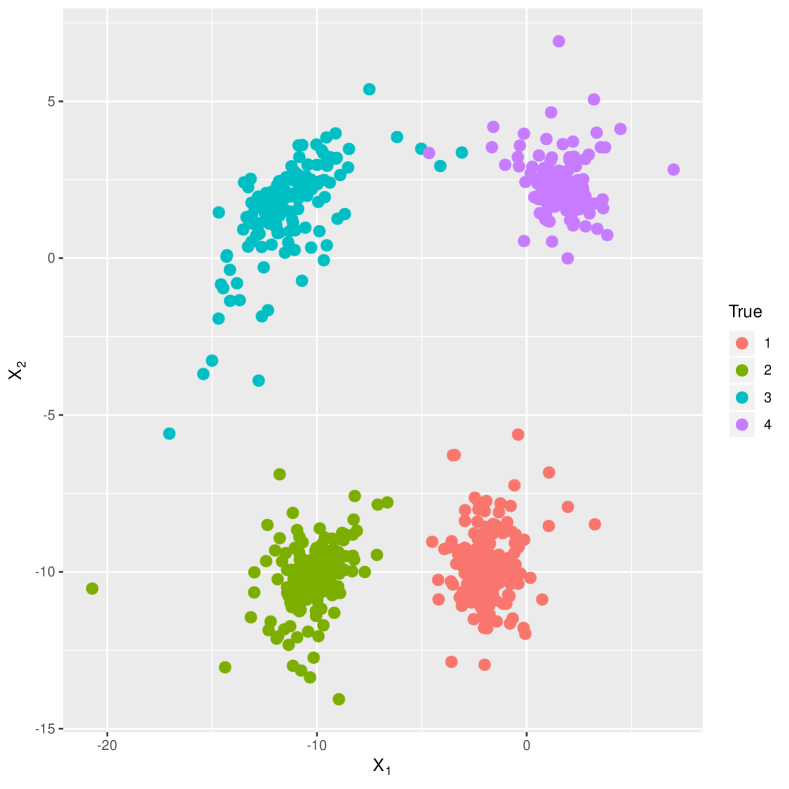
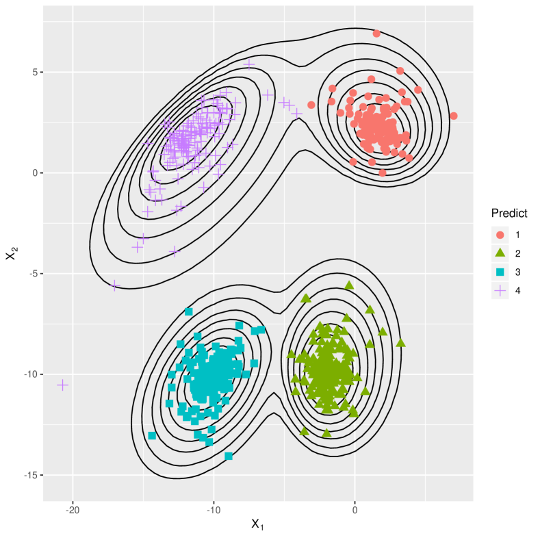
Figure 1: Scatter plot highlighting the true labels (left) and a contour plot showing the predicted classifications (right). ARI = 0.989.

In this set of simulation study, the proposed algorithm was applied to 100 two-dimensional datasets, see Figure 1 (left panel) for one of the 100 datasets. Each dataset contained a four components of skewed data with either heavier or lighter tails, whose parameters are summarized in Table 1. The number of observations in each component were not balanced i.e., the four component comprised of $200,180,150,120$ observations respectively. The proposed algorithm was applied to all 100 datasets. 100 out of 100 times it selected a four-component model and the average ARI is $0.994$ (standard error of 0.001). The estimated parameters are also summarized in Table 1.

Table 1: True and estimated values for the parameters in Simulation Study 1. Numbers in parentheses are the standard errors calculated from the replications

	Component 1 ($n_{1}=200$)		Component 2 ($n_{2}=180$)
	True Parameters	Estimated Parameters	True Parameters	Estimated Parameters
$\gamma$	$1.2$	$1.08(0.33)$	$0.8$	$0.86(0.29)$
$\mu$	$[-2,\quad-10]$	$[-2.00(0.13),\quad-10.00(0.12)]$	$[-10,\quad-10]$	$[-9.99(0.16),\quad-10.03(0.12)]$
$\beta$	$[0.1,\quad 0.2]$	$[0.09(0.20),\quad 0.17(0.20)]$	$[-0.2,\quad-0.2]$	$[-0.22(0.21),\quad-0.18(0.17)]$
$\Sigma$	$\begin{bmatrix}1.2&0\\ 0&1.2\end{bmatrix}$	$\begin{bmatrix}1.11(0.28)&0.00(0.09)\\ 0.00(0.09)&1.09(0.31)\end{bmatrix}$	$\begin{bmatrix}1&0.4\\ 0.4&1\end{bmatrix}$	$\begin{bmatrix}1.06(0.32)&0.41(0.15)\\ 0.41(0.15)&1.03(0.28)\end{bmatrix}$
Mean $\mbox{\boldmath{$\mu$}}+\frac{\mbox{\boldmath{$\beta$}}}{\gamma}$	$[-1.92,\quad-9.83]$	$[-1.92(0.07),\quad-9.84(0.08)]$	$[-10.25,\quad-10.25]$	$[-10.23(0.09),\quad-10.23(0.09)]$
Variance $\frac{\mbox{\boldmath{$\Sigma$}}}{\gamma}+\frac{\mbox{\boldmath{$\beta$}}^{\top}\beta}{\gamma^{3}}$	$\begin{bmatrix}1.01&0.01\\ 0.01&1.02\end{bmatrix}$	$\begin{bmatrix}1.11(0.20)&0.01(0.09)\\ 0.01(0.09)&1.11(0.18)\end{bmatrix}$	$\begin{bmatrix}1.33&0.58\\ 0.58&1.33\end{bmatrix}$	$\begin{bmatrix}1.43(0.26)&0.59(0.16)\\ 0.59(0.16)&1.37(0.23)\end{bmatrix}$
	Component 3 ($n_{3}=150$)		Component 4($n_{4}=120$)
	True Parameters	Estimated Parameters	True Parameters	Estimated Parameters
$\gamma$	$0.6$	$0.65(0.21)$	$1$	$1.10(0.44)$
$\mu$	$[-12,\quad 2]$	$[-11.98(0.19),\quad 2.03(0.14)]$	$[2,\quad 2]$	$[2.00(0.18),\quad 2.01(0.15)]$
$\beta$	$[0.2,\quad-0.25]$	$[0.22(0.21),\quad-0.30(0.19)]$	$[-0.2,\quad 0.2]$	$[-0.26(0.37),\quad 0.23(0.28)]$
$\Sigma$	$\begin{bmatrix}2&1\\ 1&1\end{bmatrix}$	$\begin{bmatrix}2.12(0.55)&1.05(0.29)\\ 1.05(0.29)&1.04(0.29)\end{bmatrix}$	$\begin{bmatrix}1.2&-0.2\\ -0.2&1\end{bmatrix}$	$\begin{bmatrix}1.30(0.49)&-0.22(0.14)\\ -0.22(0.14)&1.07(0.41)\end{bmatrix}$
Mean $\mbox{\boldmath{$\mu$}}+\frac{\mbox{\boldmath{$\beta$}}}{\gamma}$	$[-11.67,\quad 1.58]$	$[-11.64(0.17),\quad 1.57(0.12)]$	$[1.80,\quad 2.20]$	$[1.78(0.12),\quad 2.21(0.10)]$
Variance $\frac{\mbox{\boldmath{$\Sigma$}}}{\gamma}+\frac{\mbox{\boldmath{$\beta$}}^{\top}\beta}{\gamma^{3}}$	$\begin{bmatrix}3.52&1.44\\ 1.44&1.96\end{bmatrix}$	$\begin{bmatrix}3.93(0.78)&1.55(0.36)\\ 1.55(0.36)&2.20(0.55)\end{bmatrix}$	$\begin{bmatrix}1.24&-0.24\\ -0.24&1.04\end{bmatrix}$	$\begin{bmatrix}1.39(0.37)&-0.28(0.17)\\ -0.28(0.17)&1.13(0.26)\end{bmatrix}$

Figure 1 (left) shows the true component membership of one of the hundred datasets and Figure 1 (right) gives the contour plot based on the estimated parameters for the dataset described in the left panel. The 95% credible intervals for all parameter estimation for all 100 datasets are given in the Appendix B, where the lower and upper endpoints of the credible intervals are the empirical 0.025-percentiles and 0.975-percentiles.

We compared our approach with other commonly used mixture models: Gaussian mixture models (GMM) implemented in the R package mclust (Scrucca et al.,, 2017), and mixtures of generalized hyperbolic distributions (MixGHD; Browne and McNicholas,, 2015), which also have the flexibility of modeling skewed as well as symmetric components, and implemented in the R package MixGHD (Tortora et al.,, 2018). These mixture models were applied to all 100 datasets. Gaussian mixture models failed to capture the skewness of the components and overestimated the number of components (i.e. always selected a five or more component model) while the mixture of generalized hyperbolic distributions selected a four-component model only 77 out of 100 times and gave average ARI $=0.975$ with a standard deviation (sd) of $0.037$.

5.2 Simulation Study 2

In this simulation, 100 four-dimensional datasets were generated with three underlying groups with two components comprising of 200 observations, and the third component comprising of 100 observations. The parameters used to generate the data are summarized in Table 2. The proposed algorithm was applied to these 100 datasets and it correctly selected the correct three-component model for all 100 datasets with an average ARI of 1.000 (sd of 0.001).

Table 2: True and estimated values for the parameters in Simulation Study 2

	Component 1 ($n_{1}=100$)
	True Parameters	Estimated Parameters (Standard Error)
$\gamma$	$0.6$	$0.79(0.27)$
$\mu$	$[9,-6,-5,9]$	$[9.01(0.15),-6.00(0.16),-4.96(0.18),9.04(0.21)]$
$\beta$	$[0,0,-0.5,-0.5$	$[0.00(0.21),0.01(0.22),-0.72(0.37),-0.72(0.40)]$
$\Sigma$	$\begin{bmatrix}1&0&0&0\\ 0&1&0&0\\ 0&0&1&0\\ 0&0&0&1\end{bmatrix}$	$\begin{bmatrix}1.29(0.42)&0.02(0.17)&0.00(0.15)&0.00(0.17)\\ 0.02(0.17)&1.33(0.46)&0.02(0.16)&0.01(0.18)\\ 0.00(0.15)&0.02(0.16)&1.28(0.40)&-0.02(0.17)\\ 0.00(0.17)&0.01(0.18)&-0.02(0.17)&1.30(0.45)\end{bmatrix}$
	Component 2 ($n_{2}=200$)
	True Parameters	Estimated Parameters (Standard Error)
$\gamma$	$0.9$	$0.98(0.22)$
$\mu$	$[7,5,0,-7]$	$[6.99(0.15),4.96(0.11),-0.02(0.09),-7.00(0.13)]$
$\beta$	$[0.2,0.2,0.2,0.2]$	$[0.23(0.22),0.26(0.15),0.25(0.14),0.23(0.16)]$
$\Sigma$	$\begin{bmatrix}2&0&0&1\\ 0&1&0&0\\ 0&0&1&0\\ 1&0&0&1\end{bmatrix}$	$\begin{bmatrix}2.19(0.46)&-0.01(0.11)&-0.02(0.13)&1.10(0.24)\\ -0.01(0.11)&1.08(0.21)&0.00(0.10)&-0.01(0.09)\\ -0.02(0.13)&0.00(0.10)&1.11(0.23)&-0.02(0.09)\\ 1.10(0.24)&-0.01(0.09)&-0.02(0.09)&1.11(0.23)\end{bmatrix}$
	Component 3 ($n_{3}=200$)
	True Parameters	Estimated Parameters (Standard Error)
$\gamma$	$1.2$	$1.28(0.28)$
$\mu$	$[-3,-2,7,3]$	$[-2.97(0.25),-2.00(0.11),7.02(0.21),3.00(0.16)]$
$\beta$	$[0,0,0,0]$	$[-0.01(0.41),0.00(0.18),0.01(0.34),-0.02(0.25)]$
$\Sigma$	$\begin{bmatrix}6&-2&3&-1\\ -2&1&-1&0\\ 3&-1&4&-1\\ -1&0&-1&2\end{bmatrix}$	$\begin{bmatrix}6.48(1.37)&-2.16(0.46)&3.23(0.76)&-1.03(0.37)\\ -2.16(0.46)&1.10(0.28)&-1.08(0.27)&-0.02(0.13)\\ 3.23(0.76)&-1.08(0.27)&4.32(0.97)&-1.06(0.39)\\ -1.03(0.37)&-0.02(0.13)&-1.06(0.39)&2.17(0.51)\end{bmatrix}$

The average of the estimated parameters for all 100 datasets provided in Table 2 shows good parameter recovery. Figure 2 (right) gives the pairwise scatter plot based on the estimated parameters for this dataset where the true group labels are described in the left panel.

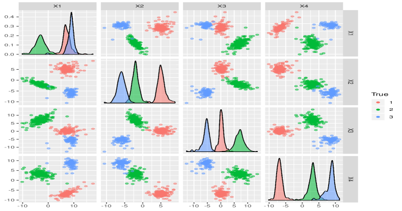
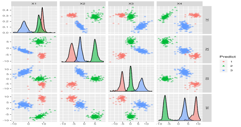
Figure 2: Pairwise scatter plot highlighting the true labels (left) and predicted classifications (right) for one of the hundred datasets. Here, the ARI was 1.

Gaussian mixture models and mixtures of generalized hyperbolic distributions were applied to these datasets. The mixture of generalized hyperbolic distributions correctly selected a three-component model for 87 out of the 100 datasets with an average ARI of $0.976$ (sd 0.066). The Gaussian mixture models only chose the correct number of components for 1 out of the 100 datasets.

5.3 Real Data Analysis

The proposed algorithm is also applied to some benchmark clustering datasets

The Crab Dataset:
This is dataset of morphological measurements on Leptograpsus crabs, available in the R package MASS (Venables and Ripley,, 2002). There are 200 observations and 5 covariates in this dataset, describing 5 morphological measurements on 50 crabs each of two colour forms and both sexes. The five measurements are frontal lobe size (FL), rear width (RW), carapace length (CL), carapace width (CW), and body depth (BD) respectively. All measurements are taken in the unit of millimeters. The proposed algorithm is applied to this dataset and it indicates a two-component model. Comparison of the estimated group membership with the two color forms of the crabs, “B” or “O” for blue or orange shows complete agreement (ARI$=1$). The pairwise scatter plots are given in Figure 3, where the left panel shows the original measurement variables and the right panel gives the principal components (only for visualization purposes), both colored with estimated classification of the color forms.

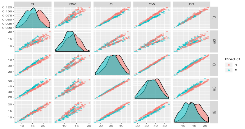
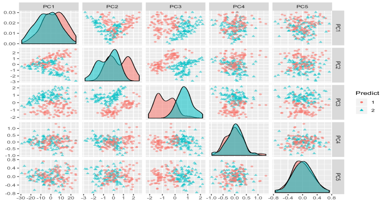
Figure 3: Pairwise scatter plot highlighting the predicted classification of the color forms of the crabs, in terms of the original measurements (left), and in terms of the principal components (right).

The Gaussian mixture models (GMM) and the mixtures of generalized hyperbolic distributions (MixGHD) were also applied to this dataset and the performance is summarized in Table 3. (IMMNIG denotes the infinite mixture of MNIG developed here) Both the mixtures of generalized hyperbolic distributions and the Gaussian mixture model select a three component model; the classification obtained by Gaussian mixture model are also more in agreement with the classification based on the gender of the crabs (ARI of 0.72) (see Table 3), whereas the estimated group membership by the mixture of generalized hyperbolic distributions are more in agreement with classifying the crabs by their sexes (ARI of 0.51) (see Table 3).

Table 3: Summary of the performances of the new model (IMMNIG), the Gaussian mixture model (GMM), and mixtures of generalized hyperbolic distributions (MixGHD) on the crabs datasets.

	Model Chosen	ARI (color)	ARI (gender)
IMMNIG	$G=2$	1.00	0.00
GMM	$G=3$	0.02	0.70
MixGHD	$G=3$	0.25	0.51

The Fish Catch Dataset
The fish catch data, available from the R package rrcov, consists of the weight and different body lengths measurements of seven different fish species. There are 159 observations in this data set. Similar to Subedi and McNicholas, (2014), after dropping the highly correlated variables, the variables Length2, Height and Width were used for the analysis where Length2 is the length from the nose to the notch of the tail, Height is the maximal height as a percentage of the length from the nose to the end of the tail, and Width is the maximal width as a percentage of the length from the nose to the end of the tail. The proposed algorithm was applied (after scaling the data) and it selected a three-component model. Figure 4 shows the pairwise scatter plots for this dataset, with the left panel showing the true species of the fish and the right panel showing the estimated component. Although the true number of species of fish is seven, from the pairwise scatter plot, it is hard to distinguish the species White, Roach and Perch; also, separation between the species Bream and Parkki, as well as between Smelt and Pike are not very clear. Table 4 summarizes the cross tabulation of the true species and estimated group membership. The GMM and mixGHD are also applied to the Fish Catch data and both resulted in a five component model with classification where the additional fifth component contained fish from both Whitewish and Perch (see Table 4 for detail). However, do note that mixGHD was able to effectively separate Smelt and Pike.

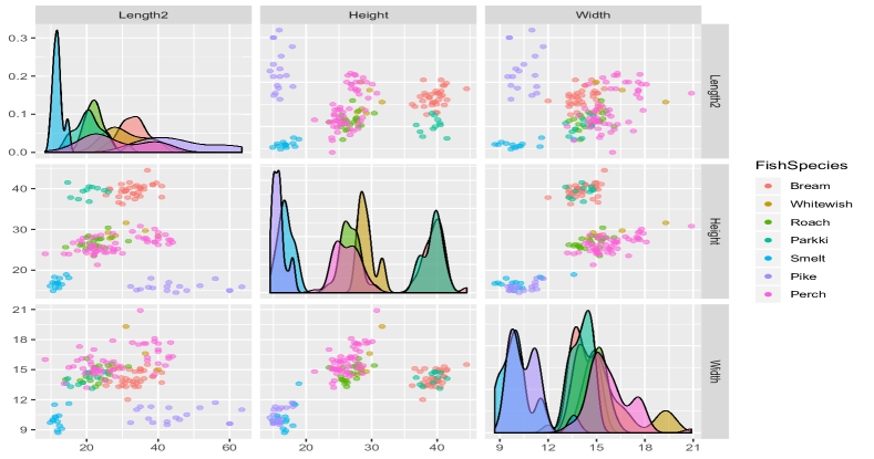
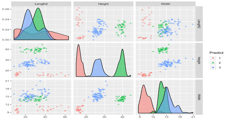
Figure 4: Pairwise scatter plot highlighting the true labels (left) and a pairwise scatter plot showing the predicted classifications (right) for the fish catch data.

Table 4: Cross tabulation of true fish species and the estimated classification using the proposed model, Gaussian mixture models, and the mixtures of generalized hyperbolic distributions.

	IMMNIG					GMM					MixGHD
	ARI: 0.59					ARI: 0.52					ARI: 0.54
	Estimated Groups					Estimated Groups					Estimated Groups
		1		2	3	1	2	3	4	5	1	2	3	4	5
Bream		34				34					34
Parkki		11				11					11
Whitewish				6			3	3				3	3
Roach				20			20					20
Perch				56			36	20				36	20
Smelt					14				11	3				14
Pike					17					17					17

The Australian Athletes (AIS) Dataset:
The AIS dataset available in the R package DAAG (Maindonald and Braun,, 2019) contains 202 observations and 13 variables comprising of measurements on various characteristics of the blood, body size, and sex of the athlete. The proposed algorithm was applied on a subset of dataset with the variables body mass index (BMI) and body fat (Bfat) as it has been previously used (Vrbik and McNicholas,, 2012; Lin,, 2010). The algorithm is applied to this dataset and a two-component model was selected. Comparing the estimated component membership with the gender yields an ARI $=0.71$. The contour plot of the fitted model in Figure 5 shows that the fitted model captured the density of the data fairly well. The Gaussian mixture models and mixtures of generalized hyperbolic distributions are also applied to the AIS dataset and the summary of the performance are given in Table 5. The Gaussian mixture model selects a three component model whereas the mixtures of generalized hyperbolic distribution selected a two component model with slightly higher classification accuracy to the proposed method.

Table 5: Summary of the performances of the proposed model, the Gaussian mixture model, and mixtures of generalized hyperbolic distributions on the AIS datasets.

	Estimated Groups	ARI
Proposed Algorithm	$G=2$	0.71
GMM	$G=3$	0.69
MixGHD	$G=2$	0.77

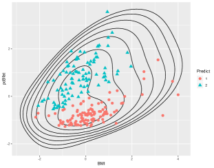
Figure 5: Contour plot using the estimated parameters for the AIS data

6 Conclusion and Discussion

In summary, a Dirichlet process mixture of MNIG distributions that can model skewness and heavy tailed data is proposed. Estimation of the posterior of the parameters and clustering was done via Gibbs sampler based on multiple layers of conjugate priors. In our framework, number of components are treated as a parameter in the model that moves freely from $1$ to $\infty$ ($N$ in practice), and are inferred during parameter estimation. This alleviates the need of choosing a model selection criteria which can be a problem. Through simulation studies, we show a near perfect classification result. Parameter estimates were very close to the true parameters and our proposed approach provides competitive results on benchmark datasets while comparing it with state-of-the art model-based clustering algorithms.

Handling of the concentration parameter $\alpha$ for the Dirichlet process prior is still an open problem that need further examination and discussion. Previous work in the context of infinite mixture of elliptical distributions, for example, Gaussian distributions, indicate that smaller $\alpha$ value will encourage the clusters to group together (West,, 1992; Escobar and West,, 1995; Gelman et al.,, 2013; Müller and Mitra,, 2013). An alternate approach is to assign a Gamma prior for $\alpha$ and update it in the Gibbs sampling framework to increase flexibility (West,, 1992; Escobar and West,, 1995). Frühwirth-Schnatter and Malsiner-Walli, (2018) in her comparison paper of Dirichlet process mixture models with sparse finite models indicates that one can reduce the prior expectation of number of components by putting a Gamma prior with larger rate parameter to $\alpha$ in the Dirichlet process mixture. We experiment the cases with different values of $\alpha$ by letting $\alpha=0.5,1,2$ and $5$, as well implementing a $Gamma(2,4)$ prior to $\alpha$ (same as Escobar and West, (1995) and Frühwirth-Schnatter and Malsiner-Walli, (2018)) for both of our simulation studies and the analysis in the fish catch data to test the robustness of clustering results to the choice of $\alpha$. The classification results in both of the simulation studies are shown to be the same. For the analysis of fish catch dataset, with the increasing of values that $\alpha$ takes, in some single Markov chain higher number of components in the model was observed; however, the final models gained when each of the three chains converged and all of them are mixed well (with a potential scale reduction factor smaller than 1.1) tend to always specify the number of clusters as 3. For the cases when algorithm utilizes a higher value of $\alpha$, it is observed that longer Markov chains are required for yielding a stable result. The interesting finding points us to some future directions, such as implementing more advanced sampling technique to improve the efficiency, and inducing some quantification for clustering stability in the Dirichlet process mixture model frameworks.

It has been observed that the Dirichlet process mixture model could overestimate the number of components, for example, Huelsenbeck and Andolfatto, (2007); Onogi et al., (2011), and Miller and Harrison, (2013). Nevertheless, both Huelsenbeck and Andolfatto, (2007) and Onogi et al., (2011) work with Dirichlet process mixture of Dirichlet distributions to specify population structures of genetic allele frequency data, in which, the overestimated number of components could due to their special structure, where the choice of concentration parameter to the base Dirichlet distribution could affect the data allocation too. Besides, the case discussed in Miller and Harrison, (2013) is very extreme and the conclusion provided is an asymptotic result. Recently, Yang et al., (2019) provide a theoretical study on the lower bounds on the ratios of posterior probability of number of components. Some future work will include filling the gap in understanding influence of choice of $\alpha$ especially in the mixture of non-elliptical distribution context.

Appendix

Appendix A Mathematical Details for Posterior Distributions

A.1 Detail on the posterior updates for the parameters

Under the Karlis and Santourian (2009) parameterization for MNIG distribution, the mean-variance mixture is of the following structure:

$$\mathbf{X}|u\sim\mathop{\rm N}(\mbox{\boldmath{$\mu$}}+u\mbox{\boldmath{$\beta$}},u\mbox{\boldmath{$\Sigma$}}),\quad U\sim\mathop{\rm IG}(1,\gamma)$$

where $\Sigma$ is not restricted. The density of MNIG distribution is of the form:

$$f_{\mathbf{X}}(\mathbf{x})=\frac{1}{2^{\frac{d-1}{2}}}\left[\frac{\alpha}{\pi q(\mathbf{x})}\right]^{\frac{d+1}{2}}\exp\left({p(\mathbf{x})}\right)~{}K_{\frac{d+1}{2}}(\alpha q(\mathbf{x}))$$

where

$$\alpha=\sqrt{\gamma^{2}+\mbox{\boldmath{$\beta$}}^{\top}\mbox{\boldmath{$\Sigma$}}^{-1}\mbox{\boldmath{$\beta$}}},\quad p(\mathbf{x})=\gamma+(\mathbf{x}-\mbox{\boldmath{$\mu$}})^{\top}\mbox{\boldmath{$\Sigma$}}^{-1}\mbox{\boldmath{$\beta$}},\quad q(\mathbf{x})=\sqrt{1+(\mathbf{x}-\mbox{\boldmath{$\mu$}})^{\top}\mbox{\boldmath{$\Sigma$}}^{-1}(\mathbf{x}-\mbox{\boldmath{$\mu$}})}$$

and $K_{d}$ is the modified Bessel function of the third kind of order $d$.

The joint probability density of $\mathbf{x}$ and $u$ is given by

$$\begin{split}f(\mathbf{x},u)=&f(\mathbf{x}|u)f(u)\\ =&(2\pi)^{-1/2}|u\mbox{\boldmath{$\Sigma$}}|^{-1/2}\exp\left\{-\frac{1}{2}(\mathbf{x}-\mbox{\boldmath{$\mu$}}-u\mbox{\boldmath{$\beta$}})^{\top}(u\mbox{\boldmath{$\Sigma$}})^{-1}(\mathbf{x}-\mbox{\boldmath{$\mu$}}-u\mbox{\boldmath{$\beta$}})\right\}\\ &\times\frac{1}{\sqrt{2\pi}}\exp(\gamma)u^{-3/2}\exp\left\{-\frac{1}{2}\left(\frac{1}{u}+\gamma^{2}u\right)\right\}\\ \propto&u^{-\frac{d+3}{2}}|\mbox{\boldmath{$\Sigma$}}|^{-1/2}\exp\left\{-\frac{1}{2}\left(\frac{1}{u}+\gamma^{2}u-2\gamma\right)-\frac{1}{2}(\mathbf{x}-\mbox{\boldmath{$\mu$}}-u\mbox{\boldmath{$\beta$}})^{\top}(u\mbox{\boldmath{$\Sigma$}})^{-1}(\mathbf{x}-\mbox{\boldmath{$\mu$}}-u\mbox{\boldmath{$\beta$}})\right\}.\end{split}$$

The complete data likelihood is of the form:

$$\begin{split}L(\theta_{g})\propto&\prod_{g=1}^{G}\prod_{i=1}^{N}\left[\pi_{g}u_{ig}^{-\frac{d+3}{2}}|\mbox{\boldmath{$\Sigma$}}_{g}|^{-\frac{1}{2}}\exp\left\{-\frac{1}{2}\left(u_{ig}^{-1}+\gamma^{2}u_{ig}-2\gamma_{g}\right)\right\}\right.\\ &\left.\times\exp\left\{-\frac{1}{2}\left(\mathbf{x}_{i}-\mbox{\boldmath{$\mu$}}_{g}-u_{ig}\mbox{\boldmath{$\beta$}}_{g})^{\top}(u_{ig}\mbox{\boldmath{$\Sigma$}}_{g})^{-1}(\mathbf{x}_{i}-\mbox{\boldmath{$\mu$}}_{g}-u_{ig}\mbox{\boldmath{$\beta$}}_{g}\right)\right\}\right]\\ =&\prod_{g=1}^{G}\left[\pi_{g}|\mbox{\boldmath{$\Sigma$}}_{g}|^{-\frac{1}{2}}\exp\left\{\gamma_{g}-\mbox{\boldmath{$\beta$}}_{g}^{\top}\mbox{\boldmath{$\Sigma$}}_{g}^{-1}\mbox{\boldmath{$\mu$}}_{g}\right\}\right]^{\sum_{i=1}^{N}{z_{ig}}}\times\prod_{g=1}^{G}\prod_{i=1}^{N}\left(u_{ig}^{-\frac{d+3}{2}}\right)^{z_{ig}}\\ &\times\prod_{g=1}^{G}\exp\left\{-\frac{1}{2}\sum_{i=1}^{N}{z_{ig}u_{ig}^{-1}\mathbf{x}_{i}^{\top}\mbox{\boldmath{$\Sigma$}}_{g}^{-1}\mathbf{x}_{i}}+\mbox{\boldmath{$\beta$}}_{g}^{\top}\mbox{\boldmath{$\Sigma$}}_{g}^{-1}\sum_{i=1}^{N}{z_{ig}\mathbf{x}_{i}}+\mbox{\boldmath{$\mu$}}_{g}^{\top}\mbox{\boldmath{$\Sigma$}}_{g}^{-1}\sum_{i=1}^{N}{z_{ig}u_{ig}^{-1}\mathbf{x}_{i}}\right.\\ &\quad\quad\quad\quad\quad\left.-\frac{1}{2}\left(\mbox{\boldmath{$\beta$}}_{g}^{\top}\mbox{\boldmath{$\Sigma$}}_{g}^{-1}\mbox{\boldmath{$\beta$}}_{g}+\gamma_{g}^{2}\right)\sum_{i=1}^{N}{z_{ig}u_{ig}}-\frac{1}{2}\left(\mbox{\boldmath{$\mu$}}_{g}^{\top}\mbox{\boldmath{$\Sigma$}}_{g}^{-1}\mbox{\boldmath{$\mu$}}_{g}+1\right)\sum_{i=1}^{N}{z_{ig}u_{ig}^{-1}}\right\}\\ =&\prod_{g=1}^{G}\left\{[r(\theta_{g})]^{t_{0g}}\cdot\prod_{i=1}^{N}[h(\mathbf{x}_{i},u_{ig})]^{z_{ig}}\times\exp Tr\left\{\sum_{j=1}^{5}\phi_{j}(\theta_{g})\mathbf{t}_{jg}(\mathbf{x},\mathbf{u}_{g})\right\}\right\}.\\ \end{split}$$

Then, common conjugate priors and their group specified posterior distributions of each parameter, $\gamma_{g},\mbox{\boldmath{$\mu$}}_{g},\mbox{\boldmath{$\beta$}}_{g},\mbox{\boldmath{$\Sigma$}}_{g}$ can be derived in the following.

• Focusing on $\gamma_{g}$, the part in the likelihood that contains $\gamma_{g}$ is as follows

  $$\begin{split}L(\gamma_{g})&\propto\left[\exp\{\gamma_{g}\}\right]^{\sum_{i=1}^{N}{z_{ig}}}\times\exp\left\{-\frac{1}{2}\sum_{i=1}^{N}{z_{ig}u_{ig}}\gamma_{g}^{2}\right\}\\ &=\exp\left\{-\frac{1}{2}\left(\sum_{i=1}^{N}{z_{ig}u_{ig}}\gamma_{g}^{2}-2\sum_{i=1}^{N}{z_{ig}}\gamma_{g}\right)\right\}=\exp\left\{-\frac{1}{2}\left(a_{3}\gamma_{g}^{2}-2a_{0}\gamma_{g}\right)\right\}.\end{split}$$

  This is a functional form of normal distribution with mean $\dfrac{a_{0}}{a_{3}}$ and variance $\dfrac{1}{a_{3}}$, truncated at 0 because we want $\gamma_{g}$ to be positive. Therefore, a conjugate truncated normal prior is assigned to $\gamma_{g}$, i.e.

  $$\gamma_{g}\sim\mathop{\rm N}\left(\frac{a_{0}^{(0)}}{a_{3}^{(0)}},\frac{1}{a_{3}^{(0)}}\right)\cdot\mathbf{1}\left(\gamma_{g}>0\right);$$

  and the resulting posterior is truncated normal as well:

  $$\gamma_{g}\sim\mathop{\rm N}\left(\dfrac{a_{0,g}}{a_{3,g}},\dfrac{1}{a_{3,g}}\right)\cdot\mathbf{1}\left(\gamma_{g}>0\right).$$

• For the precision matrix $\mbox{\boldmath{$\Sigma$}}_{g}^{-1}$, denoted as $\mathbf{T}_{g}$, in the following derivation, the part of likelihood which contains $\mathbf{T}_{g}=\mbox{\boldmath{$\Sigma$}}_{g}^{-1}$ yields the following:

  $$\begin{split}L(\mathbf{T}_{g})&\propto|\mathbf{T}_{g}|^{\sum_{i=1}^{N}{z_{ig}}/2}\cdot\exp\left\{-\frac{1}{2}Tr\left[\sum_{i=1}^{N}{z_{ig}u_{ig}^{-1}\left(\mathbf{x}_{i}-\mbox{\boldmath{$\mu$}}_{g}-u_{ig}\mbox{\boldmath{$\beta$}}_{g}\right)\left(\mathbf{x}_{i}-\mbox{\boldmath{$\mu$}}_{g}-u_{ig}\mbox{\boldmath{$\beta$}}_{g}\right)^{\top}}\mathbf{T}_{g}\right]\right\}\\ &=|\mathbf{T}_{g}|^{a_{0}/2}\exp\left\{-\frac{1}{2}Tr\left(\mathbf{V}_{0}^{-1}\mathbf{T}_{g}\right)\right\};\end{split}$$

  which is a functional form of the Wishart distribution.

  Hence, a conjugate $Wishart\left(a_{0}^{(0)},{\mathbf{a}_{5}^{(0)}}^{-1}\right)$ prior is given to $\mathbf{T}_{g}$. When computing the posterior, we take $(\mbox{\boldmath{$\mu$}}_{g},\mbox{\boldmath{$\beta$}}_{g})$ into consideration as well because they carry information about $\mathbf{T}_{g}$ and in addition, they contribute to likelihood together with $\mathbf{T}_{g}$; therefore the resulting posterior is conditional on $(\mbox{\boldmath{$\mu$}}_{g},\mbox{\boldmath{$\beta$}}_{g})$, and is of the form

  $$\mathbf{T}_{g}|(\mbox{\boldmath{$\mu$}}_{g},\mbox{\boldmath{$\beta$}}_{g})\sim Wishart(a_{0,g},\mathbf{V}_{0,g}).$$

  The derivation of the posterior parameter $\mathbf{V}_{0,g}$ is presented at the end of this section.

• Look at the pair of $(\mbox{\boldmath{$\mu$}}_{g},\mbox{\boldmath{$\beta$}}_{g})$, whose related part in the likelihood is conditional on $\mathbf{T}_{g}=\mbox{\boldmath{$\Sigma$}}_{g}^{-1}$ and is a functional form of correlated Gaussian distribution.

  $$\begin{split}L(\mbox{\boldmath{$\mu$}}_{g},\mbox{\boldmath{$\beta$}}_{g}|\mathbf{T}_{g})&\propto\exp\left\{\sum_{i=1}^{N}{z_{ig}\left(-\mbox{\boldmath{$\beta$}}_{g}^{\top}\mathbf{T}_{g}\mbox{\boldmath{$\mu$}}_{g}\right)}\right.\\ &\quad\quad\quad\quad\quad\left.-\frac{1}{2}\left[\sum_{i=1}^{N}{z_{ig}u_{ig}^{-1}\left(\mathbf{x}_{i}-\mbox{\boldmath{$\mu$}}_{g}-u_{ig}\mbox{\boldmath{$\beta$}}_{g}\right)^{\top}\mathbf{T}_{g}\left(\mathbf{x}_{i}-\mbox{\boldmath{$\mu$}}_{g}-u_{ig}\mbox{\boldmath{$\beta$}}_{g}\right)}\right]\right\}\\ &\propto\exp\left\{\mbox{\boldmath{$\beta$}}_{g}^{\top}\mathbf{T}_{g}\mbox{\boldmath{$\mu$}}_{g}\sum_{i=1}^{N}{z_{ig}}+\mbox{\boldmath{$\beta$}}_{g}^{\top}\mathbf{T}_{g}\sum_{i=1}^{N}{z_{ig}\mathbf{x}_{i}}+\mbox{\boldmath{$\mu$}}_{g}^{\top}\mathbf{T}_{g}\sum_{i=1}^{N}{z_{ig}u_{ig}^{-1}\mathbf{x}_{i}}\right.\\ &\quad\quad\quad\quad\quad\left.-\frac{1}{2}\left(\mbox{\boldmath{$\beta$}}_{g}^{\top}\mathbf{T}_{g}\mbox{\boldmath{$\beta$}}_{g}\right)\sum_{i=1}^{N}{z_{ig}u_{ig}}-\frac{1}{2}\left(\mbox{\boldmath{$\mu$}}_{g}^{\top}\mathbf{T}_{g}\mbox{\boldmath{$\mu$}}_{g}\right)\sum_{i=1}^{N}{z_{ig}u_{ig}^{-1}}\right\}.\end{split}$$

  Therefore, a multivariate normal distribution conditional on the precision matrix is assigned to $(\mbox{\boldmath{$\mu$}}_{g},\mbox{\boldmath{$\beta$}}_{g})$ such that

  $$\left.\begin{pmatrix}\mbox{\boldmath{$\mu$}}_{g}\\ \mbox{\boldmath{$\beta$}}_{g}\end{pmatrix}\right|\mathbf{T}_{g}\sim\mathop{\rm N}\left[\begin{pmatrix}\mbox{\boldmath{$\mu$}}_{0}^{(0)}\\ \mbox{\boldmath{$\beta$}}_{0}^{(0)}\end{pmatrix},\begin{pmatrix}\tau_{\mu}^{(0)}\mathbf{T}_{g}&\tau_{\mu\beta}^{(0)}\mathbf{T}_{g}\\ \tau_{\mu\beta}^{(0)}\mathbf{T}_{g}&\tau_{\beta}^{(0)}\mathbf{T}_{g}\end{pmatrix}\right];$$

  and hence the posterior is then

  $$\left.\begin{pmatrix}\mbox{\boldmath{$\mu$}}_{g}\\ \mbox{\boldmath{$\beta$}}_{g}\end{pmatrix}\right|\mathbf{T}_{g}\sim\mathop{\rm N}\left[\begin{pmatrix}\mbox{\boldmath{$\mu$}}_{0,g}\\ \mbox{\boldmath{$\beta$}}_{0,g}\end{pmatrix},\begin{pmatrix}\tau_{\mu,g}\mathbf{T}_{g}&\tau_{\mu\beta,g}\mathbf{T}_{g}\\ \tau_{\mu\beta,g}\mathbf{T}_{g}&\tau_{\beta,g}\mathbf{T}_{g}\end{pmatrix}\right].$$

  where

  $$\mbox{\boldmath{$\mu$}}_{0}^{(0)} =\frac{a_{3}^{(0)}\mathbf{a}_{2}^{(0)}-a_{0}^{(0)}\mathbf{a}_{1}^{(0)}}{a_{3}^{(0)}a_{4}^{(0)}-{a_{0}^{(0)}}^{2}}, \mbox{\boldmath{$\mu$}}_{0,g} =\frac{a_{3,g}\mathbf{a}_{2,g}-a_{0,g}\mathbf{a}_{1,g}}{a_{3,g}a_{4,g}-{a_{0,g}}^{2}};$$

  $$\mbox{\boldmath{$\beta$}}_{0}^{(0)} =\frac{a_{4}^{(0)}\mathbf{a}_{1}^{(0)}-a_{0}^{(0)}\mathbf{a}_{2}^{(0)}}{a_{3}^{(0)}a_{4}^{(0)}-{a_{0}^{(0)}}^{2}}, \mbox{\boldmath{$\beta$}}_{0,g} =\frac{a_{4,g}\mathbf{a}_{1,g}-a_{0,g}\mathbf{a}_{2,g}}{a_{3,g}a_{4,g}-{a_{0,g}}^{2}};$$

  $$\tau_{\mu}^{(0)} =a_{4}^{(0)}, \tau_{\mu,g} =a_{4,g};$$

  $$\tau_{\beta}^{(0)} =a_{3}^{(0)}, \tau_{\beta,g} =a_{3,g};$$

  $$\tau_{\mu\beta}^{(0)} =a_{0}^{(0)}, \tau_{\mu\beta,g} =a_{0,g}.$$

  Derivation of the forms of $\mbox{\boldmath{$\mu$}}_{0,g},\mbox{\boldmath{$\beta$}}_{0,g},\tau_{\mu,g},\tau_{\beta,g},$ and $\tau_{\mu\beta,g}$ is shown as the follows.

• Now, recall that the prior of $\mathbf{T}_{g}=\mbox{\boldmath{$\Sigma$}}_{g}^{-1}$ is $\mathbf{T}_{g}\sim Wishart\left(a_{0}^{(0)},{\mathbf{a}_{5}^{(0)}}^{-1}\right)$; also, conditional on $\mathbf{T}_{g}$, $(\mbox{\boldmath{$\mu$}}_{g},\mbox{\boldmath{$\beta$}}_{g})$ follows a multivariate normal distribution jointly. Consider these two prior densities jointly, we derive the updated form of $\mathbf{V}_{0,g},\mbox{\boldmath{$\mu$}}_{0,g},\mbox{\boldmath{$\beta$}}_{0,g},\tau_{\mu,g},\tau_{\beta,g},$ and $\tau_{\mu\beta,g}$.

  The joint prior density of $\mbox{\boldmath{$\mu$}}_{g},\mbox{\boldmath{$\beta$}}_{g},\mathbf{T}_{g}$ is as following:

  $$\begin{split}p(\mbox{\boldmath{$\mu$}}_{g},\mbox{\boldmath{$\beta$}}_{g},\mathbf{T}_{g})\propto\begin{vmatrix}\tau_{\mu}^{(0)}\mathbf{T}_{g}&\tau_{\mu\beta}^{(0)}\mathbf{T}_{g}\\ \tau_{\mu\beta}^{(0)}\mathbf{T}_{g}&\tau_{\beta}^{(0)}\mathbf{T}_{g}\end{vmatrix}^{-\frac{1}{2}}&\exp\left\{-\frac{1}{2}\begin{pmatrix}\mbox{\boldmath{$\mu$}}_{g}-\mbox{\boldmath{$\mu$}}_{0}^{(0)}\\ \mbox{\boldmath{$\beta$}}_{g}-\mbox{\boldmath{$\beta$}}_{0}^{(0)}\end{pmatrix}^{\top}\begin{pmatrix}\tau_{\mu}^{(0)}\mathbf{T}_{g}&\tau_{\mu\beta}^{(0)}\mathbf{T}_{g}\\ \tau_{\mu\beta}^{(0)}\mathbf{T}_{g}&\tau_{\beta}^{(0)}\mathbf{T}_{g}\end{pmatrix}\begin{pmatrix}\mbox{\boldmath{$\mu$}}_{g}-\mbox{\boldmath{$\mu$}}_{0}^{(0)}\\ \mbox{\boldmath{$\beta$}}_{g}-\mbox{\boldmath{$\beta$}}_{0}^{(0)}\end{pmatrix}\right\}\\ \times\left|\mathbf{T}_{g}\right|^{\frac{(a_{0}^{(0)}+d+1)-d-1}{2}}&\exp\left\{-\frac{1}{2}Tr\left(\mathbf{a}_{5}^{(0)}\mathbf{T}_{g}\right)\right\}\end{split}$$

  Look at the part inside the $\exp$ function only, we have a form of the following:

  $$\begin{split}&Tr\left(\mathbf{a}_{5}^{(0)}\mathbf{T}_{g}\right)+(\mbox{\boldmath{$\mu$}}_{g}-\mbox{\boldmath{$\mu$}}_{0}^{(0)})^{\top}\tau_{\mu}^{(0)}\mathbf{T}_{g}(\mbox{\boldmath{$\mu$}}_{g}-\mbox{\boldmath{$\mu$}}_{0}^{(0)})+(\mbox{\boldmath{$\beta$}}_{g}-\mbox{\boldmath{$\beta$}}_{0}^{(0)})^{\top}\tau_{\mu\beta}^{(0)}\mathbf{T}_{g}(\mbox{\boldmath{$\mu$}}_{g}-\mbox{\boldmath{$\mu$}}_{0}^{(0)})\\ &\quad\quad\quad\quad\quad+(\mbox{\boldmath{$\mu$}}_{g}-\mbox{\boldmath{$\mu$}}_{0}^{(0)})^{\top}\tau_{\mu\beta}^{(0)}\mathbf{T}_{g}(\mbox{\boldmath{$\beta$}}_{g}-\mbox{\boldmath{$\beta$}}_{0}^{(0)})+(\mbox{\boldmath{$\beta$}}_{g}-\mbox{\boldmath{$\beta$}}_{0}^{(0)})^{\top}\tau_{\beta}^{(0)}\mathbf{T}_{g}(\mbox{\boldmath{$\beta$}}_{g}-\mbox{\boldmath{$\beta$}}_{0}^{(0)})\\ =&Tr\left(\mathbf{a}_{5}^{(0)}\mathbf{T}_{g}\right)+\mbox{\boldmath{$\mu$}}_{g}^{\top}\tau_{\mu}^{(0)}\mathbf{T}_{g}\mbox{\boldmath{$\mu$}}_{g}-2\mbox{\boldmath{$\mu$}}_{g}^{\top}\tau_{\mu}^{(0)}\mathbf{T}_{g}\mbox{\boldmath{$\mu$}}_{0}^{(0)}-2\mbox{\boldmath{$\mu$}}_{g}^{\top}\tau_{\mu\beta}^{(0)}\mathbf{T}_{g}\mbox{\boldmath{$\beta$}}_{0}^{(0)}\\ &\quad\quad\quad\quad\quad+\mbox{\boldmath{$\beta$}}_{g}^{\top}\tau_{\beta}^{(0)}\mathbf{T}_{g}\mbox{\boldmath{$\beta$}}_{g}-2\mbox{\boldmath{$\beta$}}_{g}^{\top}\tau_{\beta}^{(0)}\mathbf{T}_{g}\mbox{\boldmath{$\beta$}}_{0}^{(0)}-2\mbox{\boldmath{$\beta$}}_{g}^{\top}\tau_{\mu\beta}^{(0)}\mathbf{T}_{g}\mbox{\boldmath{$\mu$}}_{0}^{(0)}\\ &\quad\quad\quad\quad\quad+2\mbox{\boldmath{$\beta$}}_{g}^{\top}\tau_{\mu\beta}^{(0)}\mathbf{T}_{g}\mbox{\boldmath{$\mu$}}_{g}+{\mbox{\boldmath{$\mu$}}_{0}^{(0)}}^{\top}\tau_{\mu}^{(0)}\mathbf{T}_{g}\mbox{\boldmath{$\mu$}}_{0}^{(0)}+2{\mbox{\boldmath{$\beta$}}_{0}^{(0)}}^{\top}\tau_{\mu\beta}^{(0)}\mathbf{T}_{g}\mbox{\boldmath{$\mu$}}_{0}^{(0)}+{\mbox{\boldmath{$\beta$}}_{0}^{(0)}}^{\top}\tau_{\beta}^{(0)}\mathbf{T}_{g}\mbox{\boldmath{$\beta$}}_{0}^{(0)}.\end{split}$$

  Now multiply the joint prior density with the likelihood that contains $\mbox{\boldmath{$\mu$}}_{g},\mbox{\boldmath{$\beta$}}_{g}$, and $\mathbf{T}_{g}$, we get the posterior. Only look at the part inside the $\exp$ again, we have the following:

  $$\begin{split}&Tr\left(\mathbf{a}_{5}^{(0)}\mathbf{T}_{g}\right)+(\mbox{\boldmath{$\mu$}}_{g}-\mbox{\boldmath{$\mu$}}_{0}^{(0)})^{\top}\tau_{\mu}^{(0)}\mathbf{T}_{g}(\mbox{\boldmath{$\mu$}}_{g}-\mbox{\boldmath{$\mu$}}_{0}^{(0)})+(\mbox{\boldmath{$\beta$}}_{g}-\mbox{\boldmath{$\beta$}}_{0}^{(0)})^{\top}\tau_{\mu\beta}^{(0)}\mathbf{T}_{g}(\mbox{\boldmath{$\mu$}}_{g}-\mbox{\boldmath{$\mu$}}_{0}^{(0)})\\ &\quad\quad\quad\quad\quad+(\mbox{\boldmath{$\mu$}}_{g}-\mbox{\boldmath{$\mu$}}_{0}^{(0)})^{\top}\tau_{\mu\beta}^{(0)}\mathbf{T}_{g}(\mbox{\boldmath{$\beta$}}_{g}-\mbox{\boldmath{$\beta$}}_{0}^{(0)})+(\mbox{\boldmath{$\beta$}}_{g}-\mbox{\boldmath{$\beta$}}_{0}^{(0)})^{\top}\tau_{\beta}^{(0)}\mathbf{T}_{g}(\mbox{\boldmath{$\beta$}}_{g}-\mbox{\boldmath{$\beta$}}_{0}^{(0)})\\ &\quad\quad\quad\quad\quad+\sum_{i=1}^{N}{z_{ig}u_{ig}^{-1}}\left(\mathbf{x}_{i}-\mbox{\boldmath{$\mu$}}_{g}-u_{ig}\mbox{\boldmath{$\beta$}}_{g}\right)^{\top}\mathbf{T}_{g}\left(\mathbf{x}_{i}-\mbox{\boldmath{$\mu$}}_{g}-u_{ig}\mbox{\boldmath{$\beta$}}_{g}\right)\\ =&Tr\left(\mathbf{a}_{5}^{(0)}\mathbf{T}_{g}\right)+\mbox{\boldmath{$\mu$}}_{g}^{\top}\tau_{\mu}^{(0)}\mathbf{T}_{g}\mbox{\boldmath{$\mu$}}_{g}-2\mbox{\boldmath{$\mu$}}_{g}^{\top}\tau_{\mu}^{(0)}\mathbf{T}_{g}\mbox{\boldmath{$\mu$}}_{0}^{(0)}-2\mbox{\boldmath{$\mu$}}_{g}^{\top}\tau_{\mu\beta}^{(0)}\mathbf{T}_{g}\mbox{\boldmath{$\beta$}}_{0}^{(0)}\\ &\quad\quad\quad\quad\quad-2\sum_{i=1}^{N}{z_{ig}u_{ig}^{-1}}\mathbf{x}_{i}\mathbf{T}_{g}\mbox{\boldmath{$\mu$}}_{g}+\mbox{\boldmath{$\mu$}}_{g}^{\top}\sum_{i=1}^{N}{z_{ig}u_{ig}^{-1}}\mathbf{T}_{g}\mbox{\boldmath{$\mu$}}_{g}\\ &\quad\quad\quad\quad\quad+\mbox{\boldmath{$\beta$}}_{g}^{\top}\tau_{\beta}^{(0)}\mathbf{T}_{g}\mbox{\boldmath{$\beta$}}_{g}-2\mbox{\boldmath{$\beta$}}_{g}^{\top}\tau_{\beta}^{(0)}\mathbf{T}_{g}\mbox{\boldmath{$\beta$}}_{0}^{(0)}-2\mbox{\boldmath{$\beta$}}_{g}^{\top}\tau_{\mu\beta}^{(0)}\mathbf{T}_{g}\mbox{\boldmath{$\mu$}}_{0}^{(0)}\\ &\quad\quad\quad\quad\quad-2\sum_{i=1}^{N}{z_{ig}\mathbf{x}_{i}^{\top}}\mathbf{T}_{g}\mbox{\boldmath{$\beta$}}_{g}+\mbox{\boldmath{$\beta$}}_{g}^{\top}\sum_{i=1}^{N}{z_{ig}u_{ig}}\mathbf{T}_{g}\mbox{\boldmath{$\beta$}}_{g}\\ &\quad\quad\quad\quad\quad+2\mbox{\boldmath{$\mu$}}_{g}^{\top}\tau_{\mu\beta}^{(0)}\mathbf{T}_{g}\mbox{\boldmath{$\beta$}}_{g}+2\mbox{\boldmath{$\mu$}}_{g}^{\top}\sum_{i=1}^{N}{z_{ig}}\mathbf{T}_{g}\mbox{\boldmath{$\beta$}}_{g}\\ &\quad\quad\quad\quad\quad+2{\mbox{\boldmath{$\mu$}}_{0}^{(0)}}^{\top}\tau_{\mu\beta}^{(0)}\mathbf{T}_{g}\mbox{\boldmath{$\beta$}}_{0}^{(0)}+{\mbox{\boldmath{$\mu$}}_{0}^{(0)}}^{\top}\tau_{\mu}^{(0)}\mathbf{T}_{g}\mbox{\boldmath{$\mu$}}_{0}^{(0)}+{\mbox{\boldmath{$\beta$}}_{0}^{(0)}}^{\top}\tau_{\beta}^{(0)}\mathbf{T}_{g}\mbox{\boldmath{$\beta$}}_{0}^{(0)}+\sum_{i=1}^{N}{z_{ig}u_{ig}^{-1}}\mathbf{x}_{i}^{\top}\mathbf{T}_{g}\mathbf{x}_{i}.\end{split}$$

  The exponential part inside the posterior density should have the same functional form as the prior, i.e., it is expected to have the form of

  $$\begin{split}&Tr\left(\mathbf{V}_{0,g}^{-1}\mathbf{T}_{g}\right)+\mbox{\boldmath{$\mu$}}_{g}^{\top}\tau_{\mu}\mathbf{T}_{g}\mbox{\boldmath{$\mu$}}_{g}-2\mbox{\boldmath{$\mu$}}_{g}^{\top}\tau_{\mu}\mathbf{T}_{g}\mbox{\boldmath{$\mu$}}_{0,g}-2\mbox{\boldmath{$\mu$}}_{g}^{\top}\tau_{\mu\beta}\mathbf{T}_{g}\mbox{\boldmath{$\beta$}}_{0,g}\\ &\quad\quad\quad\quad\quad+\mbox{\boldmath{$\beta$}}_{g}^{\top}\tau_{\beta}\mathbf{T}_{g}\mbox{\boldmath{$\beta$}}_{g}-2\mbox{\boldmath{$\beta$}}_{g}^{\top}\tau_{\beta}\mathbf{T}_{g}\mbox{\boldmath{$\beta$}}_{0,g}-2\mbox{\boldmath{$\beta$}}_{g}^{\top}\tau_{\mu\beta}\mathbf{T}_{g}\mbox{\boldmath{$\mu$}}_{0,g}\\ &\quad\quad\quad\quad\quad+2\mbox{\boldmath{$\beta$}}_{g}^{\top}\tau_{\mu\beta}\mathbf{T}_{g}\mbox{\boldmath{$\mu$}}_{g}+{\mbox{\boldmath{$\mu$}}_{0,g}}^{\top}\tau_{\mu}\mathbf{T}_{g}\mbox{\boldmath{$\mu$}}_{0,g}+2\mbox{\boldmath{$\beta$}}_{0,g}^{\top}\tau_{\mu\beta}\mathbf{T}_{g}\mbox{\boldmath{$\mu$}}_{0,g}+{\mbox{\boldmath{$\beta$}}_{0,g}}^{\top}\tau_{\beta}\mathbf{T}_{g}\mbox{\boldmath{$\beta$}}_{0,g}.\end{split}$$

  By comparing the previous two terms, we derive the following:

  $$\begin{split}\tau_{\mu,g}&=\tau_{\mu}^{(0)}+\sum_{i=1}^{N}{z_{ig}u_{ig}^{-1}}=a_{4}^{(0)}+\sum_{i=1}^{N}{z_{ig}u_{ig}^{-1}}=a_{4,g};\\ \tau_{\beta,g}&=\tau_{\beta}^{(0)}+\sum_{i=1}^{N}{z_{ig}u_{ig}}=a_{3}^{(0)}+\sum_{i=1}^{N}{z_{ig}u_{ig}}=a_{3,g};\\ \tau_{\mu\beta,g}&=\tau_{\mu\beta}^{(0)}+\sum_{i=1}^{N}{z_{ig}}=a_{0}^{(0)}+\sum_{i=1}^{N}{z_{ig}}=a_{0,g}.\end{split}$$

  Besides, we have

  $$\begin{split}&\left\{\begin{split}\tau_{\mu,g}\mathbf{T}_{g}\mbox{\boldmath{$\mu$}}_{0,g}+\tau_{\mu\beta,g}\mathbf{T}_{g}\mbox{\boldmath{$\beta$}}_{0,g}&=\tau_{\mu}^{(0)}\mathbf{T}_{g}\mbox{\boldmath{$\mu$}}_{0}^{(0)}+\tau_{\mu\beta}^{(0)}\mathbf{T}_{g}\mbox{\boldmath{$\beta$}}_{0}^{(0)}+\mathbf{T}_{g}\sum_{i=1}^{N}{z_{ig}u_{ig}^{-1}\mathbf{x}_{i}}\\ \tau_{\mu\beta,g}\mathbf{T}_{g}\mbox{\boldmath{$\mu$}}_{0,g}+\tau_{\beta,g}\mathbf{T}_{g}\mbox{\boldmath{$\beta$}}_{0,g}&=\tau_{\beta}^{(0)}\mathbf{T}_{g}\mbox{\boldmath{$\beta$}}_{0}^{(0)}+\tau_{\mu\beta}^{(0)}\mathbf{T}_{g}\mbox{\boldmath{$\mu$}}_{0}^{(0)}+\mathbf{T}_{g}\sum_{i=1}^{N}{z_{ig}\mathbf{x}_{i}}\end{split}\right.\\ \Rightarrow&\left\{\begin{split}a_{4,g}\mbox{\boldmath{$\mu$}}_{0,g}+a_{0,g}\mbox{\boldmath{$\beta$}}_{0,g}&=a_{4}^{(0)}\mbox{\boldmath{$\mu$}}_{0}^{(0)}+a_{0}^{(0)}\mbox{\boldmath{$\beta$}}_{0}^{(0)}+\sum_{i=1}^{N}{z_{ig}u_{ig}^{-1}\mathbf{x}_{i}}\\ a_{0,g}\mbox{\boldmath{$\mu$}}_{0,g}+a_{3,g}\mbox{\boldmath{$\beta$}}_{0,g}&=a_{3}^{(0)}\mbox{\boldmath{$\beta$}}_{0}^{(0)}+a_{0}^{(0)}\mbox{\boldmath{$\mu$}}_{0}^{(0)}+\sum_{i=1}^{N}{z_{ig}\mathbf{x}_{i}}\end{split}\right.\end{split};$$

  plus given that

  $$\mbox{\boldmath{$\mu$}}_{0}^{(0)}=\frac{a_{3}^{(0)}\mathbf{a}_{2}^{(0)}-a_{0}^{(0)}\mathbf{a}_{1}^{(0)}}{a_{3}^{(0)}a_{4}^{(0)}-{a_{0}^{(0)}}^{2}},\quad\quad\mbox{\boldmath{$\beta$}}_{0}^{(0)}=\frac{a_{4}^{(0)}\mathbf{a}_{1}^{(0)}-a_{0}^{(0)}\mathbf{a}_{2}^{(0)}}{a_{3}^{(0)}a_{4}^{(0)}-{a_{0}^{(0)}}^{2}},$$

  the solution to $\mbox{\boldmath{$\mu$}}_{0,g}$ and $\mbox{\boldmath{$\beta$}}_{0,g}$ is

  $$\mbox{\boldmath{$\mu$}}_{0,g}=\frac{a_{3,g}\mathbf{a}_{2,g}-a_{0,g}\mathbf{a}_{1,g}}{a_{3,g}a_{4,g}-{a_{0,g}}^{2}},\quad\quad\mbox{\boldmath{$\beta$}}_{0,g}=\frac{a_{4,g}\mathbf{a}_{1,g}-a_{0,g}\mathbf{a}_{2,g}}{a_{3,g}a_{4,g}-{a_{0,g}}^{2}}.$$

  Last, we have

  $$\begin{split}&Tr\left(\mathbf{V}_{0,g}^{-1}\mathbf{T}_{g}\right)+\mbox{\boldmath{$\mu$}}_{g}^{\top}\tau_{\mu}\mathbf{T}_{g}\mbox{\boldmath{$\mu$}}_{g}+\mbox{\boldmath{$\beta$}}_{g}^{\top}\tau_{\beta}\mathbf{T}_{g}\mbox{\boldmath{$\beta$}}_{g}+2\mbox{\boldmath{$\beta$}}_{g}^{\top}\tau_{\mu\beta}\mathbf{T}_{g}\mbox{\boldmath{$\mu$}}_{g}\\ =&Tr\left(\mathbf{a}_{5}^{(0)}\mathbf{T}_{g}\right)+2{\mbox{\boldmath{$\mu$}}_{0}^{(0)}}^{\top}\tau_{\mu\beta}^{(0)}\mathbf{T}_{g}\mbox{\boldmath{$\beta$}}_{0}^{(0)}+{\mbox{\boldmath{$\mu$}}_{0}^{(0)}}^{\top}\tau_{\mu}^{(0)}\mathbf{T}_{g}\mbox{\boldmath{$\mu$}}_{0}^{(0)}+{\mbox{\boldmath{$\beta$}}_{0}^{(0)}}^{\top}\tau_{\beta}^{(0)}\mathbf{T}_{g}\mbox{\boldmath{$\beta$}}_{0}^{(0)}+\sum_{i=1}^{N}{z_{ig}u_{ig}^{-1}}\mathbf{x}_{i}^{\top}\mathbf{T}_{g}\mathbf{x}_{i};\end{split}$$

  from which $\mathbf{V}_{0,g}^{-1}$ is shown to have the form as below:

  $$\begin{split}\mathbf{V}_{0,g}^{-1}=&\mathbf{a}_{5}^{(0)}+\sum_{i=1}^{N}{z_{ig}u_{ig}^{-1}\mathbf{x}_{i}\mathbf{x}_{i}^{\top}}\\ &+\mbox{\boldmath{$\mu$}}_{0}^{(0)}\tau_{\mu}^{(0)}{\mbox{\boldmath{$\mu$}}_{0}^{(0)}}^{\top}+\mbox{\boldmath{$\mu$}}_{0}^{(0)}\tau_{\mu\beta}^{(0)}{\mbox{\boldmath{$\beta$}}_{0}^{(0)}}^{\top}+\mbox{\boldmath{$\beta$}}_{0}^{(0)}\tau_{\mu\beta}^{(0)}{\mbox{\boldmath{$\mu$}}_{0}^{(0)}}^{\top}+\mbox{\boldmath{$\beta$}}_{0}^{(0)}\tau_{\beta}^{(0)}{\mbox{\boldmath{$\beta$}}_{0}^{(0)}}^{\top}\\ &-\left(\mbox{\boldmath{$\mu$}}_{0,g}\tau_{\mu,g}\mbox{\boldmath{$\mu$}}_{0,g}^{\top}+\mbox{\boldmath{$\mu$}}_{0,g}\tau_{\mu\beta,g}\mbox{\boldmath{$\beta$}}_{0,g}^{\top}+\mbox{\boldmath{$\beta$}}_{0,g}\tau_{\mu\beta,g}\mbox{\boldmath{$\mu$}}_{0,g}^{\top}+\mbox{\boldmath{$\beta$}}_{0,g}\tau_{\beta,g}\mbox{\boldmath{$\beta$}}_{0,g}^{\top}\right)\\ =&\mathbf{a}_{5,g}+\mbox{\boldmath{$\mu$}}_{0}^{(0)}\tau_{\mu}^{(0)}{\mbox{\boldmath{$\mu$}}_{0}^{(0)}}^{\top}+\mbox{\boldmath{$\mu$}}_{0}^{(0)}\tau_{\mu\beta}^{(0)}{\mbox{\boldmath{$\beta$}}_{0}^{(0)}}^{\top}+\mbox{\boldmath{$\beta$}}_{0}^{(0)}\tau_{\mu\beta}^{(0)}{\mbox{\boldmath{$\mu$}}_{0}^{(0)}}^{\top}+\mbox{\boldmath{$\beta$}}_{0}^{(0)}\tau_{\beta}^{(0)}{\mbox{\boldmath{$\beta$}}_{0}^{(0)}}^{\top}\\ &-\left(\mbox{\boldmath{$\mu$}}_{0,g}\tau_{\mu,g}\mbox{\boldmath{$\mu$}}_{0,g}^{\top}+\mbox{\boldmath{$\mu$}}_{0,g}\tau_{\mu\beta,g}\mbox{\boldmath{$\beta$}}_{0,g}^{\top}+\mbox{\boldmath{$\beta$}}_{0,g}\tau_{\mu\beta,g}\mbox{\boldmath{$\mu$}}_{0,g}^{\top}+\mbox{\boldmath{$\beta$}}_{0,g}\tau_{\beta,g}\mbox{\boldmath{$\beta$}}_{0,g}^{\top}\right)\\ \end{split}$$

A.2 Detail on posterior updates for hyperparameters

A.2.1 Derivation of the posteriors

There are six hyperparameters, $a_{0}^{(0)},\mathbf{a}_{1}^{(0)},\mathbf{a}_{2}^{(0)},a_{3}^{(0)},a_{4}^{(0)},$ and $\mathbf{a}_{5}^{(0)}$, common for all groups, that defines the prior distributions of the parameters. Another layer of prior distributions can be added on these hyperparameters for additional flexibility. Again, common conjugate prior distributions are assigned to these hyperparameters, which yield posteriors that depends on the group-specified observations. Details of the derivation are given below.

Again, recall that the complete data likelihood can be written into a form that comes from the exponential family:

$$L(\theta_{g})\propto\prod_{g=1}^{G}\left\{[r(\theta_{g})]^{t_{0g}}\cdot\prod_{i=1}^{N}[h(\mathbf{x}_{i},u_{ig})]^{z_{ig}}\times\exp Tr\left\{\sum_{j=1}^{5}\phi_{j}(\theta_{g})\mathbf{t}_{jg}(\mathbf{x},\mathbf{u}_{g})\right\}\right\}$$

where

$$r(\mbox{\boldmath{$\theta$}}_{g}) =\pi_{g}|\mbox{\boldmath{$\Sigma$}}_{g}|^{-\frac{1}{2}}\exp\left\{\gamma_{g}-\mbox{\boldmath{$\mu$}}_{g}^{\top}\mbox{\boldmath{$\Sigma$}}_{g}^{-1}\mbox{\boldmath{$\beta$}}_{g}\right\}, t_{0g} =\sum_{i=1}^{N}{z_{ig}};$$

$$\phi_{1}(\mbox{\boldmath{$\theta$}}_{g}) =\mbox{\boldmath{$\Sigma$}}_{g}^{-1}\mbox{\boldmath{$\beta$}}_{g}, \mathbf{t}_{1g}(\mathbf{x},\mathbf{u}_{g}) =\sum_{i=1}^{N}z_{ig}\mathbf{x}_{i}^{\top};$$

$$\phi_{2}(\mbox{\boldmath{$\theta$}}_{g}) =\mbox{\boldmath{$\Sigma$}}_{g}^{-1}\mbox{\boldmath{$\mu$}}_{g}, \mathbf{t}_{2g}(\mathbf{x},\mathbf{u}_{g}) =\sum_{i=1}^{N}z_{ig}u_{ig}^{-1}\mathbf{x}_{i}^{\top};$$

$$\phi_{3}(\mbox{\boldmath{$\theta$}}_{g}) =-\frac{1}{2}(\mbox{\boldmath{$\Sigma$}}_{g}^{-1}\mbox{\boldmath{$\beta$}}_{g}\mbox{\boldmath{$\beta$}}_{g}^{\top}+\frac{\gamma_{g}^{2}}{d}\mathbb{I}_{d}), t_{3g}(\mathbf{x},\mathbf{u}_{g}) =\sum_{i=1}^{N}z_{ig}u_{ig};$$

$$\phi_{4}(\mbox{\boldmath{$\theta$}}_{g}) =-\frac{1}{2}(\mbox{\boldmath{$\Sigma$}}_{g}^{-1}\mbox{\boldmath{$\mu$}}_{g}\mbox{\boldmath{$\mu$}}_{g}^{\top}+\frac{1}{d}\mathbb{I}_{d}), t_{4g}(\mathbf{x},\mathbf{u}_{g}) =\sum_{i=1}^{N}z_{ig}u_{ig}^{-1};$$

$$\phi_{5}(\mbox{\boldmath{$\theta$}}_{g}) =-\frac{1}{2}\mbox{\boldmath{$\Sigma$}}_{g}^{-1}, \mathbf{t}_{5g}(\mathbf{x},\mathbf{u}_{g}) =\sum_{i=1}^{N}z_{ig}u_{ig}^{-1}\mathbf{x}_{i}\mathbf{x}_{i}^{\top}.$$

• $a_{0}^{(0)}$ is associated with $t_{0g}$, who only relates to $r(\mbox{\boldmath{$\theta$}}_{g})$ in the complete data likelihood, with a functional form of the density from an exponential distribution. Therefore, an exponential prior with rate parameter $b_{0}$ is assigned to $a_{0}^{(0)}$:

  $$a_{0}^{(0)}\sim\text{Exp}(b_{0}),\quad p\left(a_{0}^{(0)}\right)=b_{0}\exp\left(-b_{0}a_{0}^{(0)}\right);$$

  hence the posterior is an exponential distribution as well with rate parameter $b_{0}-\sum_{g=1}^{G}\log(\pi_{g})-\sum_{g=1}^{G}\log\left(|\mbox{\boldmath{$\Sigma$}}_{g}|^{-\frac{1}{2}}\right)-\sum_{g=1}^{G}\gamma_{g}+\sum_{g=1}^{G}\mbox{\boldmath{$\mu$}}_{g}^{\top}\mbox{\boldmath{$\Sigma$}}_{g}^{-1}\mbox{\boldmath{$\beta$}}_{g}$:

  $$\begin{split}p\left(a_{0}^{(0)}|r(\theta_{1}),\dots r(\theta_{G})\right)&\propto\exp\left\{-b_{0}a_{0}^{(0)}\right\}\prod_{g=1}^{G}\exp\left\{\left[r(\theta_{g})\right]^{t_{0g}}\right\}\\ &=\exp\left\{-b_{0}a_{0}^{(0)}\right\}\exp\left\{\sum_{g=1}^{G}\left[\log(\pi_{g})+\log\left(|\mbox{\boldmath{$\Sigma$}}_{g}|^{-\frac{1}{2}}\right)+\gamma_{g}-\mbox{\boldmath{$\mu$}}_{g}^{\top}\mbox{\boldmath{$\Sigma$}}_{g}^{-1}\mbox{\boldmath{$\beta$}}_{g}\right]t_{0g}\right\}\\ &=\exp\left\{-\left[b_{0}-\sum_{g=1}^{G}\log(\pi_{g})-\sum_{g=1}^{G}\log\left(|\mbox{\boldmath{$\Sigma$}}_{g}|^{-\frac{1}{2}}\right)\right.\right.\\ &\quad\quad\quad\quad\quad\quad\quad\quad\left.\left.-\sum_{g=1}^{G}\gamma_{g}+\sum_{g=1}^{G}\mbox{\boldmath{$\mu$}}_{g}^{\top}\mbox{\boldmath{$\Sigma$}}_{g}^{-1}\mbox{\boldmath{$\beta$}}_{g}\right]a_{0}^{(0)}\right\}\end{split}$$

• $\mathbf{a}_{1}^{(0)}$ is associated with $\mathbf{t}_{1g}$, whose functional form in the likelihood is a multivariate Gaussian distribution and relate to $\phi_{1}(\theta_{g})$ only. A multivariate Gaussian prior is then assigned to $\mathbf{a}_{1}^{(0)}$; it yields a multivariate Gaussian posterior:

  $$\mathbf{a}_{1}^{(0)}\sim\mathop{\rm N}(\mathbf{c}_{1},B_{1}),\quad p\left(\mathbf{a}_{1}^{(0)}\right)\propto\exp\left\{-\frac{1}{2}\left(\mathbf{a}_{1}^{(0)}-\mathbf{c}_{1}\right)^{\top}B_{1}^{-1}\left(\mathbf{a}_{1}^{(0)}-\mathbf{c}_{1}\right)\right\};$$

  $$\begin{split}p\left(\mathbf{a}_{1}^{(0)}|\phi_{1}(\theta_{1}),\dots,\phi_{1}(\theta_{G})\right)&\propto\exp\left\{-\frac{1}{2}\left(\mathbf{a}_{1}^{(0)}-\mathbf{c}_{1}\right)^{\top}B_{1}^{-1}\left(\mathbf{a}_{1}^{(0)}-\mathbf{c}_{1}\right)\right\}\prod_{g=1}^{G}\exp Tr\left\{\phi_{1g}\mathbf{t}_{1g}\right\}\\ &=\exp\left\{-\frac{1}{2}\left(\mathbf{a}_{1}^{(0)}-\mathbf{c}_{1}\right)^{\top}B_{1}^{-1}\left(\mathbf{a}_{1}^{(0)}-\mathbf{c}_{1}\right)+\sum_{g=1}^{G}\mbox{\boldmath{$\beta$}}_{g}^{\top}\mbox{\boldmath{$\Sigma$}}_{g}^{-1}\mathbf{t}_{1g}\right\}\\ &=\exp\left\{-\frac{1}{2}\left[{\mathbf{a}_{1}^{(0)}}^{\top}B_{1}^{-1}\mathbf{a}_{1}^{(0)}\right.\right.\\ &\quad\quad\quad\quad\quad\quad\left.\left.-2\left(\mathbf{c}_{1}^{\top}B_{1}^{-1}+\sum_{g=1}^{G}\mbox{\boldmath{$\beta$}}_{g}^{\top}\mbox{\boldmath{$\Sigma$}}_{g}^{-1}\right)\mathbf{a}_{1}^{(0)}+\mathbf{c}_{1}B_{1}^{-1}\mathbf{c}_{1}\right]\right\}\\ &\propto\exp\left\{-\frac{1}{2}\left[\mathbf{a}_{1}^{(0)}-\left(\mathbf{c}_{1}+\sum_{g=1}^{G}\mbox{\boldmath{$\beta$}}_{g}^{\top}\mbox{\boldmath{$\Sigma$}}_{g}^{-1}B_{1}\right)B_{1}^{-1}\right]^{\top}\right.\\ &\quad\quad\quad\quad\quad\left.B_{1}^{-1}\left[\mathbf{a}_{1}^{(0)}-\left(\mathbf{c}_{1}+\sum_{g=1}^{G}\mbox{\boldmath{$\beta$}}_{g}^{\top}\mbox{\boldmath{$\Sigma$}}_{g}^{-1}B_{1}\right)B_{1}^{-1}\right]\right\}.\end{split}$$

  The mean and covariance matrix of the posterior is $\mathbf{c}_{1}+\sum_{g=1}^{G}\mbox{\boldmath{$\beta$}}_{g}^{\top}\mbox{\boldmath{$\Sigma$}}_{g}^{-1}B_{1}$ and $B_{1}$ respectively.

• Similar to $\mathbf{a}_{1}^{(0)}$, $\mathbf{a}_{2}^{(0)}$ is associated with $\mathbf{t}_{2g}$ who also possess a functional term of multivariate Gaussian that relate to the part including $\phi_{2}(\theta_{g})$ only in the likelihood. A multivariate Gaussian prior is assigned to $\mathbf{a}_{2}^{(0)}$ and results in a multivariate Gaussian posterior with mean $\mathbf{c}_{2}+\sum_{g=1}^{G}\mbox{\boldmath{$\mu$}}_{g}^{\top}\mbox{\boldmath{$\Sigma$}}_{g}^{-1}B_{2}$ and covariance $B_{2}$.

  $$\mathbf{a}_{2}^{(0)}\sim\mathop{\rm N}(\mathbf{c}_{2},B_{2}),\quad p\left(\mathbf{a}_{2}^{(0)}\right)\propto\exp\left\{-\frac{1}{2}\left(\mathbf{a}_{2}^{(0)}-\mathbf{c}_{2}\right)^{\top}B_{2}^{-1}\left(\mathbf{a}_{2}^{(0)}-\mathbf{c}_{2}\right)\right\};$$

  $$\begin{split}p\left(\mathbf{a}_{2}^{(0)}|\phi_{2}(\theta_{1}),\dots,\phi_{2}(\theta_{G})\right)&\propto\exp\left\{-\frac{1}{2}\left(\mathbf{a}_{2}^{(0)}-\mathbf{c}_{2}\right)^{\top}B_{2}^{-1}\left(\mathbf{a}_{2}^{(0)}-\mathbf{c}_{2}\right)\right\}\prod_{g=1}^{G}\exp Tr\left\{\phi_{2g}\mathbf{t}_{2g}\right\}\\ &=\exp\left\{-\frac{1}{2}\left(\mathbf{a}_{2}^{(0)}-\mathbf{c}_{2}\right)^{\top}B_{2}^{-1}\left(\mathbf{a}_{2}^{(0)}-\mathbf{c}_{2}\right)+\sum_{g=1}^{G}\mbox{\boldmath{$\mu$}}_{g}^{\top}\mbox{\boldmath{$\Sigma$}}_{g}^{-1}\mathbf{t}_{2g}\right\}\\ &=\exp\left\{-\frac{1}{2}\left[{\mathbf{a}_{2}^{(0)}}^{\top}B_{2}^{-1}\mathbf{a}_{2}^{(0)}\right.\right.\\ &\quad\quad\quad\quad\quad\quad\left.\left.-2\left(\mathbf{c}_{2}^{\top}B_{2}^{-1}+\sum_{g=1}^{G}\mbox{\boldmath{$\mu$}}_{g}^{\top}\mbox{\boldmath{$\Sigma$}}_{g}^{-1}\right)\mathbf{a}_{2}^{(0)}+\mathbf{c}_{2}B_{2}^{-1}\mathbf{c}_{2}\right]\right\}\\ &\propto\exp\left\{-\frac{1}{2}\left[\mathbf{a}_{2}^{(0)}-\left(\mathbf{c}_{2}+\sum_{g=1}^{G}\mbox{\boldmath{$\mu$}}_{g}^{\top}\mbox{\boldmath{$\Sigma$}}_{g}^{-1}B_{2}\right)B_{2}^{-1}\right]^{\top}\right.\\ &\quad\quad\quad\quad\quad\left.B_{2}^{-1}\left[\mathbf{a}_{2}^{(0)}-\left(\mathbf{c}_{2}+\sum_{g=1}^{G}\mbox{\boldmath{$\mu$}}_{g}^{\top}\mbox{\boldmath{$\Sigma$}}_{g}^{-1}B_{2}\right)B_{2}^{-1}\right]\right\}.\end{split}$$

• $a_{3}^{(0)}$ is associated with $t_{3g}$, which only related to $\phi_{3}(\theta_{g})$ in the likelihood and has a functional form of an exponential distribution; hence $a_{3}^{(0)}$ is assigned an exponential prior with a resulting posterior being exponential too.

  $$a_{3}^{(0)}\sim\text{Exp}(b_{3}),\quad p\left(a_{3}^{(0)}\right)=b_{3}\exp\left(-b_{3}a_{3}^{(0)}\right);$$

  $$\begin{split}p\left(a_{3}^{(0)}|\phi_{3}(\theta_{1}),\dots\phi_{3}(\theta_{G})\right)&\propto\exp\left\{-b_{3}a_{3}^{(0)}\right\}\prod_{g=1}^{G}\exp\left\{\phi_{3g}t_{3g}\right\}\\ &=\exp\left\{-\left[b_{3}-\frac{1}{2}\sum_{g=1}^{G}\left(\beta_{g}^{\top}\mbox{\boldmath{$\Sigma$}}_{g}^{-1}\beta_{g}+\gamma_{g}^{2}\right)\right]a_{3}^{(0)}\right\};\end{split}$$

  where in the posterior distribution, the rate parameter is $b_{3}-\frac{1}{2}\sum_{g=1}^{G}\left(\mbox{\boldmath{$\beta$}}_{g}^{\top}\mbox{\boldmath{$\Sigma$}}_{g}^{-1}\mbox{\boldmath{$\beta$}}_{g}+\gamma_{g}^{2}\right)$.

• Similar to $a_{3}^{(0)}$, $a_{4}^{(0)}$ is assigned an exponential prior:

  $$a_{4}^{(0)}\sim\text{Exp}(b_{4}),\quad p\left(a_{4}^{(0)}\right)=b_{4}\exp\left(-b_{4}a_{4}^{(0)}\right);$$

  $$\begin{split}p\left(a_{4}^{(0)}|\phi_{4}(\theta_{1}),\dots,\phi_{4}(\theta_{G})\right)&\propto\exp\left\{-b_{4}a_{4}^{(0)}\right\}\prod_{g=1}^{G}\exp\left\{\phi_{4g}t_{4g}\right\}\\ &=\exp\left\{-\left[b_{4}-\frac{1}{2}\sum_{g=1}^{G}\left(\mbox{\boldmath{$\mu$}}_{g}^{\top}\mbox{\boldmath{$\Sigma$}}_{g}^{-1}\mbox{\boldmath{$\mu$}}_{g}+1\right)\right]a_{4}^{(0)}\right\}.\end{split}$$

  It indicates that the posterior is exponential distribution with rate $b_{4}-\frac{1}{2}\sum_{g=1}^{G}\left(\mbox{\boldmath{$\mu$}}_{g}^{\top}\mbox{\boldmath{$\Sigma$}}_{g}^{-1}\mbox{\boldmath{$\mu$}}_{g}+1\right)$.

• $\mathbf{a}_{5}^{(0)}$ is associated with $\mbox{\boldmath{$\Sigma$}}_{g}^{-1}$. A Wishart prior is assigned to $\mathbf{a}_{5}^{(0)}$; the resulting posterior is also a Wishart distribution.

  $$\mathbf{a}_{5}^{(0)}\sim Wishart(\nu_{0},\mbox{\boldmath{$\Lambda$}}_{0}),\quad p\left(\mathbf{a}_{5}^{(0)}\right)\propto\left|\mathbf{a}_{5}^{(0)}\right|^{\frac{\nu_{0}-d-1}{2}}\exp\left\{-\frac{1}{2}Tr\left(\mbox{\boldmath{$\Lambda$}}_{0}^{-1}\mathbf{a}_{5}^{(0)}\right)\right\}$$

  The priors of $\mbox{\boldmath{$\Sigma$}}_{g}^{-1}$ perform as the likelihood in the derivation of the posterior of $\mathbf{a}_{5}^{(0)}$:

  $$\begin{split}p\left(\left.\mathbf{a}_{5}^{(0)}\right|\mbox{\boldmath{$\Sigma$}}_{1}^{-1},\dots,\mbox{\boldmath{$\Sigma$}}_{G}^{-1}\right)&\propto\left|\mathbf{a}_{5}^{(0)}\right|^{\frac{\nu_{0}-d-1}{2}}\exp\left\{-\frac{1}{2}Tr\left(\mbox{\boldmath{$\Lambda$}}_{0}^{-1}\mathbf{a}_{5}^{(0)}\right)\right\}\times\prod_{g=1}^{G}\left|\mathbf{a}_{5}^{(0)}\right|^{\frac{a_{0}^{(0)}}{2}}\exp\left\{-\frac{1}{2}Tr\left(\mathbf{a}_{5}^{(0)}\mbox{\boldmath{$\Sigma$}}_{g}^{-1}\right)\right\}\\ &=\left|\mathbf{a}_{5}^{(0)}\right|^{\frac{\nu_{0}+G\times a_{0}^{(0)}-d-1}{2}}\exp\left\{-\frac{1}{2}Tr\left[\left(\mbox{\boldmath{$\Lambda$}}_{0}^{-1}+\sum_{g=1}^{G}\mbox{\boldmath{$\Sigma$}}_{g}^{-1}\right)\mathbf{a}_{5}^{(0)}\right]\right\}\end{split}$$

  Therefore, the posterior of $\mathbf{a}_{5}^{(0)}$ is $Wishart\left[\nu_{0}+G\times a_{0}^{(0)},\left(\mbox{\boldmath{$\Lambda$}}_{0}^{-1}+\sum_{g=1}^{G}\mbox{\boldmath{$\Sigma$}}_{g}^{-1}\right)^{-1}\right]$

A.2.2 Choice of third layer hyperparameters

The third layer hyperparameters $b_{0},c_{1},B_{1},c_{2},B_{2},b_{3},b_{4},\nu_{0}$ and $\mbox{\boldmath{$\Lambda$}}_{0}$ are chosen such that if a sample is drawn from the posteriors of the hyperparameters $a_{0}^{(0)},\mathbf{a}_{1}^{(0)},\mathbf{a}_{2}^{(0)},a_{3}^{(0)},a_{4}^{(0)}$ and $\mathbf{a}_{5}^{(0)}$, it is expected to close to the associated term of $t_{0g},\mathbf{t}_{1g},\mathbf{t}_{2g},t_{3g},t_{4g}$ when $g=G=1$ and the sample covariance matrix $\mbox{\boldmath{$\Sigma$}}_{\mathbf{x}}$, respectively. Therefore, we have the following:
When $G=1$, $z_{1}=z_{2}=\cdots=z_{N}$ hence $z_{ig}=1$ when $i=g$ and $z_{ig}=0$ for $\forall i\neq g$.

$$1/b_{0} =\mathbb{E}\left(a_{0}^{(0)}\right)\sim\sum_{i=1}^{N}{z_{ig}}=N, \to\quad\quad b_{0} =1/N;$$

$$1/b_{3} =\mathbb{E}\left(a_{3}^{(0)}\right)\sim\sum_{i=1}^{N}{z_{ig}u_{ig}}, \to\quad\quad b_{3} =1/\sum_{i=1}^{N}{u_{i}};$$

$$1/b_{4} =\mathbb{E}\left(a_{4}^{(0)}\right)\sim\sum_{i=1}^{N}{z_{ig}u_{ig}^{-1}}, \to\quad\quad b_{4} =1/\sum_{i=1}^{N}{u_{i}^{-1}};$$

$$\mathbf{c}_{1} =\mathbb{E}\left(\mathbf{a}_{1}^{(0)}\right)\sim\sum_{i=1}^{N}{z_{ig}\mathbf{x}_{i}} \to\quad\quad\mathbf{c}_{1} =\sum_{i=1}^{N}{\mathbf{x}_{i}},B_{1}=\mbox{\boldmath{$\Sigma$}}_{\mathbf{x}};$$

$$\mathbf{c}_{2} =\mathbb{E}\left(\mathbf{a}_{2}^{(0)}\right)\sim\sum_{i=1}^{N}{z_{ig}u_{ig}^{-1}\mathbf{x}_{i}} \to\quad\quad\mathbf{c}_{2} =\sum_{i=1}^{N}{u_{i}^{-1}\mathbf{x}_{i}},B_{2}=\mbox{\boldmath{$\Sigma$}}_{u^{-1}\mathbf{x}};$$

$$\nu_{0}\mbox{\boldmath{$\Lambda$}}_{0} =\mathbb{E}\left(\mathbf{a}_{5}^{(0)}\right)\sim\mbox{\boldmath{$\Sigma$}}_{\mathbf{x}} \to\quad\quad\mbox{\boldmath{$\Lambda$}}_{0} =\mbox{\boldmath{$\Sigma$}}_{\mathbf{x}}/\nu_{0},\nu_{0}=d+1.$$

Appendix B Credible Intervals for Simulation Study 1

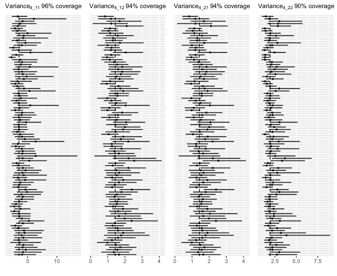
Figure 6: 95% Credible Intervals for estimated parameters for all 100 runs for Simulation Study 1.

References

• Antoniak, (1974) Antoniak, C. E. (1974). Mixtures of dirichlet processes with applications to bayesian nonparametric problems. The Annals of Statistics, 2(6):1152–1174.
• Barndorff-Nielsen, (1997) Barndorff-Nielsen, O. E. (1997). Normal inverse Gaussian distributions and stochastic volatility modelling. Scandinavian Journal of Statistics, 24(1):1–13.
• Blackwell, (1973) Blackwell, David; MacQueen, J. B. (1973). Ferguson distributions via Polya urn schemes. The Annals of Statistics, 1(2):353–355.
• Blei et al., (2017) Blei, D. M., Kucukelbir, A., and McAuliffe, J. D. (2017). Variational inference: A review for statisticians. Journal of the American Statistical Association, 112(518):859–877.
• Browne and McNicholas, (2015) Browne, R. P. and McNicholas, P. D. (2015). A mixture of generalized hyperbolic distributions. The Canadian Journal of Statistics, 43(2):176–198.
• Celeux et al., (2000) Celeux, G., Hurn, M., and Robert, C. P. (2000). Computational and inferential difficulties with mixture posterior distributions. Journal of the American Statistical Association, 95(451):957–970.
• Dellaportas and Papageorgiou, (2006) Dellaportas, P. and Papageorgiou, I. (2006). Multivariate mixtures of normals with unknown number of components. Statistics and Computing, 16(1):57–68.
• Diebolt and Robert, (1994) Diebolt, J. and Robert, C. P. (1994). Estimation of finite mixture distributions through Bayesian sampling. Journal of the Royal Statistical Society: Series B (Statistical Methodology), 56(2):363–375.
• Escobar and West, (1995) Escobar, M. D. and West, M. (1995). Bayesian density estimation and inference using mixtures. Journal of the American Statistical Association, 90(430):577–588, https://www.tandfonline.com/doi/pdf/10.1080/01621459.1995.10476550.
• Ferguson, (1973) Ferguson, T. S. (1973). A Bayesian analysis of some nonparametric problems. The Annals of Statistics, 1(2):209–230.
• Frühwirth-Schnatter, (2006) Frühwirth-Schnatter, S. (2006). Finite mixture and Markov switching models. Springer Science & Business Media.
• Frühwirth-Schnatter and Malsiner-Walli, (2018) Frühwirth-Schnatter, S. and Malsiner-Walli, G. (2018). From here to infinity: sparse finite versus Dirichlet process mixtures in model-based clustering. Advances in Data Analysis and Classification, 13:1–32.
• Fruhwirth-Schnatter and Pyne, (2010) Fruhwirth-Schnatter, S. and Pyne, S. (2010). Bayesian inference for finite mixtures of univatiate and multivariate skew-normal and skew-t distributions. Biostatistics, 11(2):317–336.
• Gelman et al., (2013) Gelman, A., Carlin, J. B., Stern, H. S., Dunson, D. B., Vehtari, A., and Rubin, D. B. (2013). Bayesian Data Analysis. CRC Press, third edition.
• Gelman et al., (1992) Gelman, A., Rubin, D. B., et al. (1992). Inference from iterative simulation using multiple sequences. Statistical Science, 7(4):457–472.
• Hakguder et al., (2018) Hakguder, Z., Shu, J., Liao, C., Pan, K., and Cui, J. (2018). Genome-scale microrna target prediction through clustering with dirichlet process mixture model. BMC Genomics, 19.
• Hejblum et al., (2019) Hejblum, B. P., Alkhassim, C., Gottardo, R., Caron, F., Thiébaut, R., et al. (2019). Sequential Dirichlet process mixtures of multivariate skew $t$-distributions for model-based clustering of flow cytometry data. The Annals of Applied Statistics, 13(1):638–660.
• Hubert and Arabie, (1985) Hubert, L. and Arabie, P. (1985). Comparing partitions. Journal of Classification, 2(1):193–218.
• Huelsenbeck and Andolfatto, (2007) Huelsenbeck, J. P. and Andolfatto, P. (2007). Inference of population structure under a dirichlet process model. Genetics, 175(4):1787–1802, https://www.genetics.org/content/175/4/1787.full.pdf.
• Ishwaran and James, (2001) Ishwaran, H. and James, L. F. (2001). Gibbs sampling methods for stick-breaking priors. Journal of the American Statistical Association, 96(453):161–173, https://doi.org/10.1198/016214501750332758.
• Karlis and Santourian, (2009) Karlis, D. and Santourian, A. (2009). Model-based clustering with non-elliptically contoured distributions. Statistics and Computing, 19(1):73–83.
• Lartillot and Philippe, (2004) Lartillot, N. and Philippe, H. (2004). A Bayesian mixture model for across-site heterogeneities in the amino-acid replacement process. Molecular Biology and Evolution, 21(6):1095–1109, http://oup.prod.sis.lan/mbe/article-pdf/21/6/1095/13413709/msh112.pdf.
• Lin, (2010) Lin, T. I. (2010). Robust mixture modeling using multivariate skew $t$ distributions. Statistics and Computing, 20:343–356.
• (24) Lin, T. I., Lee, J. C., and Hsieh, W. J. (2007a). Robust mixture modeling using the skew $t$ distribution. Statistics and Computing, 17:81–92.
• (25) Lin, T. I., Lee, J. C., and Yen, S. Y. (2007b). Finite mixture modeling using the skew normal distribution. Statistica Sinica, 17:909–927.
• Maceachern and Müller, (1998) Maceachern, S. N. and Müller, P. (1998). Estimating mixture of Dirichlet process models. Journal of Computational and Graphical Statistics, 7(2):223–238, https://www.tandfonline.com/doi/pdf/10.1080/10618600.1998.10474772.
• Maindonald and Braun, (2019) Maindonald, J. H. and Braun, W. J. (2019). DAAG: Data Analysis and Graphics Data and Functions. R package version 1.22.1.
• McNicholas et al., (2017) McNicholas, S. M., McNicholas, P. D., and Browne, R. P. (2017). A mixture of variance-gamma factor analyzers. In Big and Complex Data Analysis, pages 369–385. Springer.
• Medvedovic and Sivaganesan, (2002) Medvedovic, M. and Sivaganesan, S. (2002). Bayesian infinite mixture model based clustering of gene expression profiles. Bioinformatics, 18(9):1194–1206, http://oup.prod.sis.lan/bioinformatics/article-pdf/18/9/1194/555335/181194.pdf.
• Miller and Harrison, (2013) Miller, J. W. and Harrison, M. T. (2013). A simple example of Dirichlet process mixture inconsistency for the number of components. In Burges, C. J. C., Bottou, L., Welling, M., Ghahramani, Z., and Weinberger, K. Q., editors, Advances in Neural Information Processing Systems 26, pages 199–206. Curran Associates, Inc.
• Müller and Mitra, (2013) Müller, P. and Mitra, R. (2013). Bayesian nonparametric inference – why and how. Bayesian Anal., 8(2):269–302.
• Murray et al., (2014) Murray, P. M., Browne, R. P., and McNicholas, P. D. (2014). Mixtures of skew-$t$ factor analyzers. Computational Statistics & Data Analysis, 77:326–335.
• Neal, (2000) Neal, R. M. (2000). Markov chain sampling methods for dirichlet process mixture models. Journal of Computational and Graphical Statistics, 9(2):249–265, https://www.tandfonline.com/doi/pdf/10.1080/10618600.2000.10474879.
• O’Hagan et al., (2016) O’Hagan, A., Murphy, T. B., Gormley, I. C., McNicholas, P. D., and Karlis, D. (2016). Clustering with the multivariate normal inverse Gaussian distribution. Computational Statistics & Data Analysis, 93:18–30.
• Onogi et al., (2011) Onogi, A., Nurimoto, M., and Morita, M. (2011). Characterization of a Bayesian genetic clustering algorithm based on a Dirichlet process prior and comparison among Bayesian clustering methods. BMC bioinformatics, 12:263.
• Protassov, (2004) Protassov, R. S. (2004). EM-based maximum likelihood parameter estimation for multivariate generalized hyperbolic distributions with fixed $\lambda$. Statistics and Computing, 14(1):67–77.
• Pyne et al., (2009) Pyne, S., Hu, X., Wang, K., Rossin, E., Lin, T.-I., Baecher-Allan, L. M. M. C., McLachlan, G. J., Tamayo, P., Hafler, D. A., Jager, P. L. D., and Mesirov, J. P. (2009). Automated high-dimensional flow cytometric data analysis. Proceedings of the National Academy of Sciences, 106(27):8519–8524.
• Rasmussen, (2000) Rasmussen, C. E. (2000). The infinite Gaussian mixture model. Advances in Neural Information Processing Systems, 12:554–560.
• Richarson and Green, (1997) Richarson, S. and Green, P. J. (1997). On Bayesian analysis of mixtures with an unknown number of components. Journal of the Royal Statistical Society: Series B (Statistical Methodology), 59(4):731–792.
• Schwarz, (1978) Schwarz, G. (1978). Estimating the dimension of a model. The Annals of Statistics, 6(2):461–464.
• Scrucca et al., (2017) Scrucca, L., Fop, M., Murphy, T. B., and Raftery, A. E. (2017). mclust 5: clustering, classification and density estimation using Gaussian finite mixture models. The R Journal, 8(1):205–233.
• Sethuraman, (1994) Sethuraman, J. (1994). A constructive definition of Dirichlet priors. Statistica Sinica, 4(2):639–650.
• Stephens, (2000) Stephens, M. (2000). Dealing with label switching in mixture models. Journal of Royal Statistical Society. Series B (Methodoloty), 62(4):795–809.
• Subedi and McNicholas, (2014) Subedi, S. and McNicholas, P. D. (2014). Variational Bayes approximations for clustering via mixtures of normal inverse Gaussian distributions. Advances in Data Analysis and Classification, 8(2):167–193.
• Sun et al., (2016) Sun, J., Herazo-Maya, J., Kaminski, N., Zhao, H., and Warren, J. (2016). A dirichlet process mixture model for clustering longitudinal gene expression data. Statistics in Medicine, 36.
• Titterington et al., (1985) Titterington, D. M., Smith, A. F., and Makov, U. E. (1985). Statistical analysis of finite mixture distributions. Wiley,.
• Tortora et al., (2018) Tortora, C., ElSherbiny, A., Browne, R. P., Franczak, B. C., , McNicholas, P. D., and D.., A. D. (2018). MixGHD: Model Based Clustering, Classification and Discriminant Analysis Using the Mixture of Generalized Hyperbolic Distributions. R package version 2.2.
• Venables and Ripley, (2002) Venables, W. N. and Ripley, B. D. (2002). Modern Applied Statistics with S. Springer, New York, fourth edition. ISBN 0-387-95457-0.
• Vrbik and McNicholas, (2012) Vrbik, I. and McNicholas, P. (2012). Analytic calculations for the EM algorithm for multivariate skew-$t$ mixture models. Statistics & Probability Letters, 82(6):1169–1174.
• Wei and Li, (2012) Wei, X. and Li, C. (2012). The infinite student’s t-mixture for robust modeling. Signal Processing, 92(1):224 – 234.
• Wei et al., (2019) Wei, Y., Tang, Y., and McNicholas, P. D. (2019). Mixtures of generalized hyperbolic distributions and mixtures of skew-$t$ distributions for model-based clustering with incomplete data. Computational Statistics & Data Analysis, 130:18–41.
• West, (1992) West, M. (1992). Hyperparameter estimation in dirichlet process mixture models. Technical report, Institute of Statistics and Decision Sciences, Duke University, Durham NC 27706, USA.
• Yang et al., (2019) Yang, C.-Y., Ho, N., and Jordan, M. I. (2019). Posterior distribution for the number of clusters in Dirichlet process mixture models. ArXiv, abs/1905.09959.