Taking advantage of multiplet structure for lineshape analysis in Fourier space

Abstract

Lineshape analysis is a recurrent and often computationally intensive task in optics, even more so for multiple peaks in the presence of noise. We demonstrate an algorithm which takes advantage of peak multiplicity ($N$) to retrieve line shape information. The method is exemplified via analysis of Lorentzian and Gaussian contributions to individual lineshapes for a practical spectroscopic measurement and benefits from a linear increase in sensitivity with the number $N$. The robustness of the method and its benefits in terms of noise reduction and order of magnitude improvement in run-time performance are discussed.

I Introduction

Analysis of signal lineshapes is a prominent problem and a theme of importance in physics, chemistry and biomedicine. Ranging from spectroscopy [1, 2, 3] to scattering techniques [4, 5, 6, 7], the lineshape can reveal underlying physical processes. For example, relaxation dynamics very commonly give rise to exponential decays in time which correspond in spectroscopy to Lorentzian peaks in frequency, while static disorder and instrumental effects typically induce Gaussian distributions of characteristic frequencies. Together, the two phenomena yield signal lineshapes which are convolutions of Lorentzians with Gaussians, objects referred to as Voigt lineshapes. The accurate parametrization of a Voigt lineshape retrieves the Lorentzian contribution which e.g. quantifies correlation lengths in X-ray and neutron scattering [7] and coherence times of quantum systems in frequency-dependent spectroscopy [8, 9, 10]; and the Gaussian part which is due to extrinsic factors such as grain size distribution in x-ray diffraction [6, 11] and to spatial inhomogeneity in optical spectroscopy [2, 12].
Approaches to lineshape determination deal with efficient numeric approximations [13, 14] or tackle the deconvolution of single peaks in Fourier space [15]. However, the calculation and fitting of a Voigt profile remains computationally intensive. In case of finite-periodic signals, frequently encountered e.g. for electronic multiplets of ions in solids [16] or rotational spectra of molecules [17, 18, 19], the problem is exacerbated by the need to sum over Voigt profiles.
In this article we extend previous work on single Voigt analysis (see [15] for an overview) and exploit the regular spacing for a robust and direct determination of the individual lineshape in Fourier space. We fit an exponential to the envelope of the Fourier transform of the signal, which is parametrized only by the Lorentzian and Gaussian contribution to the individual line width. The method quantifies these contributions without the need for involved multi-Voigt profile analysis. Results are also readily checked by direct visual inspection of the Fourier transform. Furthermore, our method is computationally less expensive and it’s sensitivity increases linearly in $N$, the number of profiles. Although we focus on the common case of Voigt-shaped profiles, we expect our method will prove advantageous for other line-profiles, such as listed in refrence [20], as well.
We first derive the mathematical foundations of the method in section II. In section III we apply the procedure to typical experimental data from solid-state spectroscopy, in this case a rare-earth doped crystal. Finally, in section IV we discuss the method’s performance when the initial assumption of regular spacing is relaxed.

II Derivation of the Method

We consider a real, finite-periodic signal $S({{x}})=\sum_{i}S_{i}(x)$, consisting of $N$ profiles $S_{i}(x)$ spaced by $\Delta{{x}}$. We focus on the common cases of individual signal profiles $S_{i}(x)$ of Lorentzian, Gaussian and Voigt shapes. The general case for other classes of lineshapes is addressed subsequently.

II.1 Dirac delta model

For simplicity we first model $S({{x}})$ as a series of $N$ Dirac delta functions $\delta({{x}})$, with $N$ even, symmetrically disposed around ${{x}}=0$. Definitions and a detailed derivation are in section A and B of the Appendix. The Fourier transform $\mathcal{F}:{{x}}\rightarrow k$ applied to the Dirac model $S_{\mathrm{D}}({{x}})$ is given by

$$\begin{split}\mathcal{F}_{\mathrm{D}}=\mathcal{F}[S_{\mathrm{D}}({{x}})]=\frac{A}{\sqrt{2\pi}}\frac{\mathrm{sin}(N\Delta xk/2)}{\mathrm{sin}(\Delta xk/2)}\end{split}$$ (1)

where $A$ represents the integrated area of an individual signal profile. Figure 1 shows the amplitude spectrum $|\mathcal{F}_{\mathrm{D}}|$ ,

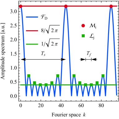
Figure 1: Amplitude spectrum $|\mathcal{F}_{\mathrm{D}}|$ of signal $S_{\mathrm{D}}(x)$ for $N=8$ and $A=1$ (blue). The maxima $\mathcal{M}_{i}$ for $i\in\{1,2,3\}$ are depicted in red and the inferior local maxima $\mathcal{L}_{j}$ in green. The uniformity of the amplitude of the $\mathcal{M}_{i}$ is highlighted by the constant red line at $8/\sqrt{2\pi}$, with spacing $T_{s}$ and the minimal amplitude $\mathcal{L}_{j,\mathrm{min}}$ by the constant green line at $\sim 1/\sqrt{2\pi}$, spaced by $T_{f}$. The limits of $\mathcal{M}_{i}$ and $\mathcal{L}_{j,\mathrm{min}}$ are derived from equation 1.

which exhibits a long periodicity $T_{s}=2\pi/\Delta{{x}}$ modulated by a short periodicity $T_{f}=T_{s}/N$. Note the frequency doubling of $|\mathcal{F}_{\mathrm{D}}|$ w.r.t $\mathcal{F}_{\mathrm{D}}$. The occurrence of $T_{s}$ in $|\mathcal{F}_{\mathrm{D}}|$ stems from the regular spacing of the $S_{i}(x)$, and $T_{f}$ from the length of the multiplet signal, which can be understood as the product of a rectangular window function with a Dirac comb (details in Appendix C) in analogy to the result of an $N-$periodic diffraction grating [21]. We denote the $i$-th maximum of $|\mathcal{F}_{\mathrm{D}}|$ as $\mathcal{M}_{i}$, i.e. $|\mathcal{F}_{\mathrm{D}}(i\times T_{s})|=\mathcal{M}_{i}~{}\forall i\in\mathbb{N}_{0}$. The inferior local maxima are labeled by $\mathcal{L}_{j}$. From equation 1 we obtain $\mathcal{M}_{i}\propto N$ for $\Delta{{x}k/2}~{}\mathrm{mod}~{}\pi=0$ with the rule of Bernoulli-de l’Hôspital and $\mathcal{L}_{j,\mathrm{min}}=1/\sqrt{2\pi}$ does not depend on the multiplet number $N$. $\mathcal{M}_{i}\propto N$ represents the scaling of the sensitivity of our Fourier lineshape analysis (FLA) method.

II.2 Lorentzian and Gaussian lineshapes

We continue for Lorentzian-shaped signal lines $S_{i}(x)=L({{x}})$, as illustrated in figure 2(a) and 2(b) for $N=8$.

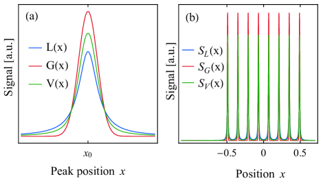
Figure 2: Signal $S(x)$ lineshape illustrations. (a) Lorentzian $L(x)$ (blue), Gaussian $G(x)$ (red) and Voigt $V(x)$ (green) lineshape with identical center $x_{0}$, area and FWHM. (b) Sum of eight equally spaced Lorentzian $L(x)$, Gaussian $G(x)$ and Voigt $V(x)$ profiles, each with identical area and FWHM.

The shape is given by

$$L({{x}},{{x}}_{0},\Gamma,A)=\frac{A}{2\pi}\frac{\Gamma}{({{x}}-{{x}}_{0})^{2}+(\frac{1}{2}\Gamma)^{2}}$$ (2)

with full-width-at-half-maximum (FWHM) $\Gamma$, center peak coordinate ${{x}}_{0}$ and integrated area $A=\int_{-\infty}^{\infty}L({{x}})\mathrm{d}{{x}}$. An $N$-fold repeated signal with spacing $\Delta{{x}}$ is represented by

$$S_{\mathrm{L}}({{x}})=\sum_{n=({1-N})/{2}}^{(N-1)/2}L({{x}},x_{0}+n\Delta{{x}},\Gamma,A)$$ (3)

and its Fourier transform $\mathcal{F}_{\mathrm{L}}=\mathcal{F}[S_{\mathrm{L}}({{x}})]$ as

$$\mathcal{F}_{\mathrm{L}}=\mathrm{exp}\left(-\frac{1}{2}\Gamma k\right)\times\frac{A}{\sqrt{2\pi}}\frac{\mathrm{sin}(N\Delta xk/2)}{\mathrm{sin}(\Delta xk/2)}$$ (4)

for $x_{0}=0$. We see that $\mathcal{F}_{\mathrm{L}}$ (eq. 4) differs from $\mathcal{F}_{\mathrm{D}}$ (eq. 1) but by an exponentially decaying prefactor

$$\mathcal{F}_{\mathrm{L}}=\mathrm{exp}\left(-\frac{1}{2}\Gamma k\right)\times\mathcal{F}_{\mathrm{D}}.$$ (5)

Figure 3 visualizes this result for $N=8$.

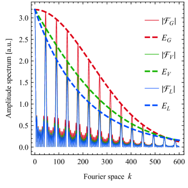
Figure 3: Fourier transform of the signal functions shown in figure 2(b). $|\mathcal{F}_{\mathrm{L}}|$ (blue), $|\mathcal{F}_{\mathrm{G}}|$ (red) and $|\mathcal{F}_{\mathrm{V}}|$ (green). The first few $\mathcal{M}_{k,i}$ are depicted for all three cases, together with the envelopes (dashed, corresponding color) defining their amplitudes.

The zero-order maximum $\mathcal{M}_{k,0}$ exhibits the same amplitude as for equation 1 but the amplitudes $\mathcal{M}_{i}$ for $i>0$ decay with $E_{\mathrm{L}}(k)=\mathrm{exp}({-\frac{1}{2}\Gamma k})$ and the sensitivity $\mathcal{M}_{i}\propto N$ of $\mathcal{F}_{\mathrm{D}}$ still holds. In the same way we obtain for a Gaussian model $S_{G}(x)$

$$\mathcal{F}_{\mathrm{G}}=\mathcal{F}\left[S_{\mathrm{G}}({{x}})\right]=\mathrm{exp}\left(-\frac{1}{2}\sigma^{2}k^{2}\right)\times\mathcal{F}_{\mathrm{D}}$$ (6)

which again exhibits the same periodicity $T_{s}$ as equation 1 and equation 4. The exponential prefactor defining the envelope $E_{\mathrm{G}}(k)$ of $\mathcal{F}_{\mathrm{G}}$ is now given by $E_{\mathrm{G}}(k)=\mathrm{exp}({-\frac{1}{2}\sigma^{2}k^{2}})$. The amplitude reduction of $\mathcal{M}_{i}$ for $i>0$ thus depends on $\sigma$ which is related to the Gaussian FWHM

$$f_{\mathrm{G}}=2\sqrt{2\mathrm{ln}(2)}\sigma.$$ (7)

II.3 Voigt profile model

The Voigt lineshape $V({{x}})$ is defined as the convolution $(*)$ of a Lorentzian with a Gaussian function:

$$V({{x}})=L({{x}})*G({{x}})=\int_{-\infty}^{\infty}L({{x}}^{\prime})G({{x}}-{{x}}^{\prime})\mathrm{d}{{x}}^{\prime}.$$ (8)

and equivalently

$$S_{\mathrm{V}}(x)=\sum_{n=({1-N})/{2}}^{(N-1)/2}V(x,x_{0}-n\Delta x,\Gamma,\sigma,A).$$ (9)

We find for $\mathcal{F}_{\mathrm{V}}=\mathcal{F}[S_{\mathrm{V}}({{x}})]$ (c.f. Appendix D)

$$\mathcal{F}_{\mathrm{V}}=\mathrm{exp}\left[-\frac{1}{2}(\Gamma+\sigma^{2}k)k\right]\times\mathcal{F}_{\mathrm{D}}$$ (10)

and observe that the sensitivity $\mathcal{M}_{i}\propto N$ still holds. Due to the convolution theorem the envelope $E_{\mathrm{V}}(k)$ defining the amplitudes of the $\mathcal{M}_{i}$ is given by

$$E_{\mathrm{V}}(k)=E_{\mathrm{L}}(k)E_{\mathrm{G}}(k)=\mathrm{exp}\left[-\frac{1}{2}(\Gamma+\sigma^{2}k)k\right]$$ (11)

which is only parametrized by the Lorentzian line width $\Gamma$ and the Gaussian $\sigma$. For illustration, figure 3 shows this for $N=8$, in addition to the Lorentzian and Gaussian cases. The Voigt FWHM $f_{\mathrm{V}}$ can be approximated with an accuracy of 0.02% [22] by

$$f_{\mathrm{V}}=0.5346f_{\mathrm{L}}+\sqrt{0.2166f_{\mathrm{L}}^{2}+f_{\mathrm{G}}^{2}}$$ (12)

where $f_{\mathrm{L}}$ denotes the Lorentzian FWHM $(f_{\mathrm{L}}=\Gamma)$.
Given a finite-periodic signal $S({{x}})$ consisting of $N$ Voigt-profile peaks $S_{i}(x)$, spaced by $\Delta{{x}}$, the line width contributions $\Gamma,\sigma$ of the individual signal peaks $S_{i}(x)$ can thus be determined by fitting $E_{\mathrm{V}}(k)$ to the $\mathcal{M}_{i}$, allowing to distinguish the Lorentzian contribution to the line width from that due to the Gaussian. From equation 10 and figure 3 the behavior of $\mathcal{F}_{\mathrm{V}}$ is dominated by $E_{\mathrm{L}}(k)$ for small $k$ and by $E_{\mathrm{G}}(k)$ for large $k$, which allows for a quick qualitative analysis of the Lorentzian contribution by examination of the first few $\mathcal{M}_{i}$ - even by eye. In principle this applies also to the strong suppression or the slow decay of the tail by $E_{\mathrm{G}}(k)$ and $E_{\mathrm{L}}(k)$ respectively, but might not be unambiguously determined due to noise.

II.4 Sensitivity and generalization of the method

The Fourier transform simplifies the convolution integral to a product and thus, the number of profiles can be understood as the number of terms of a discrete Fourier transform leading to an increase of the sensitivity, linearly in $N$ (see equation 21 in the Appendix). This point of view can be taken in analogy to the $N-$periodic diffraction grating the $\mathcal{M}_{i}$ become more expressed and sharpen as $N$ increases with the limit of becoming the Dirac comb for $N\rightarrow\infty$. This allows us to extract values for $\mathcal{M}_{i}$ even if $\mathcal{L}_{j}$ is below the noise level in the experimental setup. Thus, our result is particularly interesting for experimental applications where $N$ is large, although the case for small $N$ or even $N=1$ (c.f. reference [15]) is possible, but not recommended.
Thanks to the simplification of the convolution integral and the linear increase in sensitivity with $N$, our method applied to other classes of line-profiles [20] which are convolutions of two or more functions, should be as beneficial as for the Voigt profile. However, to which accuracy would have to be analyzed for each case separately.

III Example

In this section we demonstrate the application of the proposed method to a multiplet signal, which in this case is a typical absorbance spectrum measured in transmission for a LiY_1-xHo_xF₄ single crystal with $x=0.25\%$ at a temperature $T$ of $3.8$ K with a Fourier transform infrared (FTIR) spectrometer. The Bruker IFS125 spectrometer is based at the infrared beamline of the Swiss Light Source at Paul Scherrer Institut in Villigen, Switzerland [23]. The spectrum in figure 4(a) shows the hyperfine-split ground state to second excited state transition at $\sim 23.3$ cm^-1 (700 GHz) in spectroscopic units [cm^-1]. Thanks to the ultra-high resolution FTIR in combination with the highly collimated, high-brillance infrared beam we achieved 0.001 cm^-1 (30 MHz) resolution. We refer to Matmon et al. [16] for details on the general experimental setup and FTIR technique as well as for more extensive, spectroscopic work on LiY_1-xHo_xF₄.

III.1 Procedure

Equation 10 leads to an algorithmic procedure for extracting the shape- and line width of a finite-periodic signal:

1. Calculate the Fourier transform of the finite-periodic signal and take the modulus.

2. Determine the maxima $\mathcal{M}_{i}$ defining the envelope $E_{\mathrm{V}}(k)$, which occur with periodicity $T_{s}$.

3. Fit the envelope function

   $$E_{\mathrm{V}}(k,\Gamma,\sigma,P,c)=P\times\mathrm{exp}\left[{-\frac{1}{2}(\Gamma+\sigma^{2}k)k}\right]+c$$ (13)

   to the $\mathcal{M}_{i}$.

We replace the analytical prefactor $|\mathcal{F}_{\mathrm{D}}|$ of the envelope with $P$ as the global scaling factor, combining factors from the normalization of the Fourier transform, the single signal line area $A$ and experimental sensitivities. The offset constant $c$ accounts for nonzero white noise in the experiment. We note that if $\Delta x$ is known, the $\mathcal{M}_{i}$ might be more precisely determined thanks to $T_{s}=2\pi/\Delta x$. This simple procedure allows for algorithmic implementation.

III.2 Application to experimental data

We apply the above procedure to the transmission spectrum in figure 4(a). More details on the numerical discrete Fourier transform (DFT) procedure are found in the Appendix E. Figure 4(b) shows the modulus of the DFT coefficients $c_{k}$ of the unapodized (blue) and apodized (red) spectrum (details of apodization are in Appendix E) in figure 4(a) for $k<600$. The characteristic pattern of equation 10 is evident in figure 4. The inset displays all Fourier coefficients. We observe reduced noise frequencies in $k$-space in figure 4(b) for the apodized spectrum and a different global scaling factor $P$ with respect to the unapodized spectrum. However, the decay constants $\Gamma,\sigma$ are unchanged.
Figure 5 shows the DFT of the apodized spectrum and the $\mathcal{M}_{i}$. We apply a simple algorithm detecting the evenly spaced maxima $\mathcal{M}_{i}$ with period $T_{s}\sim 45$ Fourier coefficients. We set a conservative threshold at $k=520$ to ensure a fiducial selection of the $\mathcal{M}_{i}$. We drop $\mathcal{M}_{k,0}$ as it is strongly affected by the Fourier transforms zero center peak. The result of the envelope $E(\Gamma,\sigma,P)$ fit for a Lorentzian, Gaussian and Voigt lineshape to the $\mathcal{M}_{i}$ is displayed in figure 5. We observe that the Voigt profile yields the best results with $\Gamma=1.1\times 10^{-2}\pm 0.12\times 10^{-3}$ cm^-1 and $\sigma=3.5\times 10^{-3}\pm 0.6\times 10^{-3}$ cm^-1. With equation 7 we find $f_{\mathrm{G}}=8.5\times 10^{-3}\pm 1.4\times 10^{-3}$ cm^-1 and with equation 12 $f_{\mathrm{V}}=15.7\times 10^{-3}\pm 1.6\times 10^{-3}$ cm^-1. The same values within the fit precision are obtain by a direct Voigt profile fit to the individual signal peaks. The method determines that $f_{\mathrm{L}}$, the homogeneous part of the line width, is the slightly larger contribution.

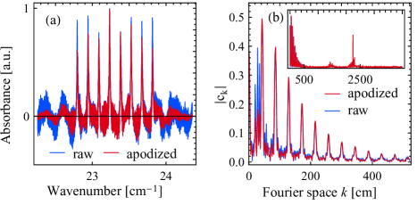
Figure 4: (a) Unapodized and apodized absorbance spectrum of LiY_1-xHo_xF₄ ($x=0.3\%$) at a temperature T = 3.8 K, exhibiting an eightfold repeated signal due to the I = 7/2 nuclear hyperfine levels of the Ho atoms. The BH4T apodization function is centered to the spectrum and decays to zero on its ends. (b) DFT coefficient $|c_{k}|$ of data shown in (a). Inset: The characteristic pattern decays within the first 600 Fourier components. Around $k=1440$ and $k=2240$ strong noise contributions from Fabry-Perot interference on reflecting optical components are visible.

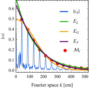
Figure 5: Modulus of Fourier coefficients of apodized spectrum in figure 4 (a) (blue). Red points denote the selected $\mathcal{M}_{i}$. Solid lines represent the envelope fit.

IV Robustness, noise stability and run time

We discuss the robustness of the method under deviations to the initial assumption of regular spacing and compare its performance to a direct least-squares fit method (DFM).

IV.1 Robustness

We examine the sensitivity of the fitting method to deviations from our initial assumption of finite-periodicity. In the case of unequal areas $A_{i}$, the individual area $A_{i}$ of the signal lines appear as an overall scaling factor which is already considered in section III. This allows the application of the method in cases where the individual signal line varies strongly in intensity e.g. for rotational/vibrational spectra [19]. The extracted line width in case of differing individual line widths $\Gamma_{i},\sigma_{i}$ is a weighted average.
As regular spacing is the underlying assumption, a variation of the line spacing $\Delta{{x}}$ directly modifies the $\mathcal{M}_{i}$ and thus the observed envelope $E(\Gamma,\sigma,P)$. Because of the line spacing variation the $N$ frequencies exhibit phase differences resulting in destructive interference and less expressed $\mathcal{M}_{i}$ (c.f. Appendix B). This leads to an overestimation of the width and deviation from actual profile shape. We note that a second order hyperfine interaction in the example spectrum (for details see [16]) results in a 2.7 % deviation from equidistancy of the eight hyperfine lines. Nevertheless we obtain equivalent results for line width and shape, showing the robustness of the method against small (on the scale of $\lesssim\Delta{{x}}/N$) relaxation in finite-periodicity of $\lesssim 3\%$. Furthermore, if the variations $\Delta{{x}}_{i}$ are known, then $E(\Gamma,\sigma,P)$ could be adjusted to depend on the $\Delta{{x}}_{i}$.

IV.2 Noise-stability

The noise spectrum is explicitly revealed with the FLA method. In case of a few isolated frequencies, as in e.g. the inset in figure 4, the noise does not affect the envelope fit in $k$-space and the method naturally implements a low-pass frequency filter. A particular strength of the method is that if there are a few frequencies between the $\mathcal{M}_{i}$ where there are what appear to be noise peaks, as is the case in figure 4 at e.g. $k=70$. Such noise peaks will affect the DFM results and low-pass filters can not be applied. Consideration only of the primary peaks at $\mathcal{M}_{i}$ provides an impartial filter of the associated noise
Assuming Gaussian RMS noise for artificial spectra with up to 50% of the signal amplitude, we find the FLA method to be comparable to DFM within the statistical parameter errors (c.f. Appendix F). This holds true for different ratios of $\Gamma/\sigma\in{0.1,1,10}$. We find that the precision for both, FLA and DFM strongly decreases for $\Gamma/\sigma<0.1$ and $\Gamma/\sigma>10$. We observe a systematic error for the FLA method in the form of an increase of the Gaussian line width contribution with increasing RMS noise amplitude. We attribute this to the fact that our analysis in Fourier space reflects the noise spectrum convolved with the signal and thus adds to the Gaussian line width contribution. Although the DFM method may occasionally exhibit a more precise performance, the FLA method extracts line width and shape information algorithmically, with less computational power and fewer data points, as detailed in the next subsection.

IV.3 Run time

We note the significantly different computational intensity of both methods. On our system (Intel(R) Xeon(R) E5-2670 0 @2.6 GHz, 2 processors with 192 GB usable RAM) DFM is at least one to two orders of magnitude slower than the FLA method. A test on 1000 data sets with $N=8$ peaks, 1000 data points, and varying Gaussian RMS noise yielded 1.6 s run time for the FLA method and 2543 s for DFM. Runtimes are dataset specific and further (algorithm) optimization may reduce the run time discrepancy. For fundamental reasons, however, a run time difference will persist as the FLA method allows to reduce the parameter space to four $(\Gamma,\sigma,P,c)$, whereas a direct fit method has to consider at least six ($\Gamma,\sigma$,area $A$, position $x_{0}$, spacing $s$, offset $c$) under the assumption of identical areas $A_{i}$, which is rarely fulfilled. Any individual consideration of a parameter in the direct fit scales the parameter space with $N$. This increases the run time for the DFM method significantly. Furthermore, the final envelope fit is performed on a fraction of the initial data points. In case of insufficient precision of the FLA method, it may well serve as a fast pre-analysis for good DFM start parameters.

V Conclusion

We have introduced and demonstrated a method of extracting the line-width and shape of a multiplet signal. The basic idea and mathematics are actually straightforward generalizations of the Debye-Waller effect [24] in scattering techniques, where the intensities of Bragg peaks shrink with increasing order in proportion to an envelope function decaying as a Gaussian whose width in reciprocal space is inversely proportional to the uncertainty in the positions of the atoms in real space. We offer a direct and computationally efficient way of quantifying the Lorentzian and Gaussian parts of multiple Voigt profiles by harnessing the regular spacing of the signal. The method benefits from a linear increase in sensitivity with the number of profiles of the multiplet. Furthermore, we highlighted that the FLA method is comparable to a direct least square fit, but is less computationally intensive and exhibits significant advantages in the presence of low-frequency noise. Finally, the FLA method might serve as a fast and algorithmic pre-analysis for starting parameter determination cases where the assumption of periodic repetition of the same lineshape is broken. Potential applications are ample. X-ray scattering may benefit where quasiperiodic structures are sampled within finite real space windows for problems such as integrated circuit microscopy [25, 26]. Our method could also be applied to optical comb-based spectroscopies [27] for precision measurements in atomic and solid-state physics.

Appendix

A Definitions

The Fourier transform we use throughout the article is defined as

$$\mathcal{F}[S({{x}})]=1/\sqrt{2\pi}\int_{-\infty}^{\infty}S({{x}})\mathrm{exp}[-ik{{x}}]\mathrm{d}{{x}}$$ (14)

We use the following definition of a Dirac comb :

$${}_{\Delta x}(x)=\frac{1}{\Delta x}\Sha\left(\frac{x}{\Delta x}\right)=\sum_{n=-\infty}^{\infty}\delta(x-n\Delta x)$$ (15)

where $\delta(x)$ denotes the Dirac delta function. The Fourier series of the Dirac comb is given by

$$\begin{split}{}_{\Delta x}(x)=\frac{1}{\sqrt{2\pi}}\sum_{n=-\infty}^{\infty}\mathrm{exp}({-ikn\Delta x})=\frac{1}{\sqrt{2\pi}}\left[1+2\sum_{n=1}^{\infty}\mathrm{cos}({kn\Delta x})\right]\end{split}$$ (16)

which directly yields another interpretation of equation 1: It is the sum of the first $N$ terms of the Fourier series of the Dirac comb ${}_{\Delta x}(x)$ for odd $N$.
The rectangular window function of height $h$ and width $w$ is defined as

$$\mathrm{rect}(h,w)=h\times\mathrm{rect}\left(\frac{x}{w}\right)$$ (17)

where we use the standard definition for the unit rectangular function $\mathrm{rect}(x)=1~{}\forall x\in\{-1/2,1/2\}$ and 0 otherwise.
The model where the individual signal peaks $S_{i}(x)=G({{x}})$ are Gaussian (c.f. figure 2(a) and (b) ) is given by

$$S_{\mathrm{G}}({{x}})=\frac{A}{\sqrt{2\pi}\sigma}\sum_{n=({1-N})/{2}}^{(N-1)/2}\mathrm{exp}\left[-\frac{({{x}}-x_{0}-n\Delta{{x}})^{2}}{2\sigma^{2}}\right]$$ (18)

with standard deviation $\sigma$, center signal line position $x_{0}$, spacing $\Delta{{x}}$ and integrated area $A$. The Fourier transform of $S_{\mathrm{G}}({{x}})$ (with $x_{0}=0$) is given by

$$\mathcal{F}_{\mathrm{G}}=\mathcal{F}\left[S_{\mathrm{G}}({{x}})\right]=\mathrm{exp}\left(-\frac{1}{2}\sigma^{2}k^{2}\right)\mathcal{F}_{\mathrm{D}}$$ (19)

B Detailed derivation

The Dirac model $S_{\mathrm{D}}({{x}})$ is given by

$$S_{\mathrm{D}}({{x}})=A\sum_{n=({1-N})/{2}}^{(N-1)/2}\delta({{x}}-n\Delta{{x}})$$ (20)

assuming symmetry around ${{x}}=0$. With $\{A,n,\Delta{{x}},k\}\in\mathbb{R}$ we obtain for $\mathcal{F}_{\mathrm{D}}$

$$\begin{split}\mathcal{F}_{\mathrm{D}}=\frac{1}{\sqrt{2\pi}}\int_{-\infty}^{\infty}A\sum_{n=({1-N})/{2}}^{(N-1)/2}\delta({{x}}-n\Delta{{x}})\times\mathrm{exp}({-ikx})~{}\mathrm{d}x=\frac{A}{\sqrt{2\pi}}\sum_{n=({1-N})/{2}}^{(N-1)/2}\mathrm{exp}({-ikn\Delta x})\end{split}$$ (21)

which, for $N$ even yields

$$\begin{split}\mathcal{F}_{\mathrm{D}}\overset{N~{}\mathrm{even}}{=}\frac{A}{\sqrt{2\pi}}\sum_{n=1/2}^{(N-1)/2}\mathrm{exp}({-ikn\Delta x})+\mathrm{exp}({ikn\Delta x})=A\sqrt{\frac{2}{\pi}}\sum_{n=1/2}^{(N-1)/2}\mathrm{cos}(n\Delta xk)\end{split}$$ (22)

and for odd $N$

$$\begin{split}\mathcal{F}_{\mathrm{D}}\overset{N~{}\mathrm{odd}}{=}\frac{A}{\sqrt{2\pi}}\sum_{n=0}^{(N-1)/2}\mathrm{exp}({-ikn\Delta x})+\mathrm{exp}({ikn\Delta x})=A\sqrt{\frac{2}{\pi}}\left[\frac{1}{2}+\sum_{n=0}^{(N-1)/2}\mathrm{cos}(n\Delta xk)\right]\end{split}$$ (23)

For even $N$ we further use

$$\begin{split}&\sum_{n=1/2}^{(N-1)/2}\mathrm{cos}(n\Delta xk)=\sum_{n=0}^{N/2-1}\mathrm{cos}\left[\left(n+\frac{1}{2}\right)\Delta xk\right]=\sum_{n=0}^{N/2-1}\mathrm{Re}\left\{\mathrm{exp}\left[i\left(n+\frac{1}{2}\right)\Delta xk\right]\right\}\\ &=\mathrm{Re}\left[\mathrm{exp}\left(\frac{i\Delta xk}{2}\right)\sum_{n=0}^{N/2-1}\mathrm{exp}\left(in\Delta xk\right)\right]=\mathrm{Re}\left[\mathrm{exp}\left(\frac{i\Delta xk}{2}\right)\frac{1-\mathrm{exp}(iN\Delta xk)}{1-\mathrm{exp}(i\Delta xk)}\right]\\ &=\mathrm{Re}\left[\mathrm{exp}\left(\frac{iN\Delta xk}{4}\right)\frac{\mathrm{exp}\left(-\frac{iN\Delta xk}{4}\right)-\mathrm{exp}\left(\frac{iN\Delta xk}{4}\right)}{\mathrm{exp}\left(-\frac{i\Delta xk}{2}\right)-\mathrm{exp}\left(\frac{i\Delta xk}{2}\right)}\right]\\ &=\frac{\mathrm{cos}(N\Delta xk/4)\mathrm{sin}(N\Delta xk/4)}{\mathrm{sin}(\Delta xk/2)}=\frac{\mathrm{sin}(N\Delta xk/2)}{\mathrm{sin}(\Delta xk/2)}\end{split}$$ (24)

and we leave the case for the odd $N$ to the reader. From equation 22 we conclude that

$$\begin{split}\mathcal{F}_{\mathrm{D}}=\frac{A}{\sqrt{2\pi}}\frac{\mathrm{sin}(N\Delta xk/2)}{\mathrm{sin}(\Delta xk/2)}~{}\forall N\geq 2\in\mathbb{N}.\end{split}$$ (25)

Equation 25 shows that the number of signal lines $N$ of $S({{x}})$ determines the amplitude of the $\mathcal{M}_{i}=NA/\sqrt{2\pi}~{}\forall i$. This is determined with the rule of Bernoulli-de l’Hôspital where numerator $[\mathrm{sin}(N\Delta xk/2)]$ and denominator $[\mathrm{sin}(\Delta xk/2)]$ vanish which is the case for $\Delta{{x}k/2}~{}\mathrm{mod}~{}\pi=0$. Furthermore, $\mathcal{L}_{\mathrm{j}}\sim A/\sqrt{2\pi}~{}\forall j$ as $\mathcal{L}_{j,\mathrm{min}}$ denotes the point where numerator and denominator are equal to one. Note that for even $N$ this condition is never exactly met and $\mathcal{L}_{j,\mathrm{min}}$ slightly smaller than 1 but still independent of $N$. These results lead to

$$\frac{\mathcal{M}_{i}}{\mathcal{L}_{j,\mathrm{min}}}\propto N$$ (26)

which is the scaling of the sensitivity of the FLA method with the number $N$ of individual signal profiles $S_{i}(x)$, in analogy to a finite diffraction grating. This result can be alternatively understood as the approximate ratio of the main maximum to the first side lobe of a sinc-function, as shown in the next subsection.

C Alternative derivation

A sum of $N$ delta functions centered around 0 and spaced by $\Delta x$ can be written as

$$\begin{split}S_{\mathrm{D}}({{x}})=&A\sum_{n=({1-N})/{2}}^{(N-1)/2}\delta({{x}}-n\Delta{{x}})~{}\forall N\in\mathbb{N}\geq 2\end{split}$$ (27)

or as

$$S_{\mathrm{D}}({{x}})=A{}_{\Delta x}(x)\mathrm{rect}\left(\frac{x}{N\Delta x}\right)~{}\forall N\in\mathbb{N}\geq 2$$ (28)

For $\mathcal{F}[S_{\mathrm{D}}({{x}})]\equiv\mathcal{F}_{\mathrm{D}}$ follows with the application of the convolution theorem:

$$\begin{split}\mathcal{F}_{\mathrm{D}}&=A\mathcal{F}\left[{}_{\Delta x}(x)\mathrm{rect}\left(\frac{x}{N\Delta x}\right)\right]=A\mathcal{F}\left[{}_{\Delta x}(x)\right]*\mathcal{F}\left[\mathrm{rect}\left(\frac{x}{N\Delta x}\right)\right]\\ &=\frac{A}{\Delta x}{}_{\frac{1}{\Delta x}}(k)*\frac{N\Delta x}{\sqrt{2\pi}}\mathrm{sinc}\left(\frac{N\Delta x}{2}k\right)=\frac{AN}{\sqrt{2\pi}}\sum_{m=-\infty}^{\infty}\mathrm{sinc}\left[\frac{N\Delta x}{2}\left(k-\frac{m}{\Delta x}\right)\right]\end{split}$$ (29)

which reveals equation 1 to be an infinite sum of sinc functions.

D Detailed derivation of Voigt model

We present the detailed derivation for $\mathcal{F}_{\mathrm{V}}$.

$$\begin{split}\mathcal{F}_{\mathrm{V}}&=\mathcal{F}\left[\sum_{n=({1-N})/{2}}^{(N-1)/2}V(x,x_{0}-n\Delta x,\Gamma,\sigma,A)\right]=\sum_{n=({1-N})/{2}}^{(N-1)/2}\mathcal{F}\left[V(x,x_{0}-n\Delta x,\Gamma,\sigma,A)\right]\\ &=\sum_{n=({1-N})/{2}}^{(N-1)/2}\mathcal{F}\left[L(x,x_{0}-n\Delta x,\Gamma,A)*G(x,0,\sigma,1)\right]\\ &=\sum_{n=({1-N})/{2}}^{(N-1)/2}\mathcal{F}\left[L(x,x_{0}-n\Delta x,\Gamma,A)\right]\times\mathcal{F}\left[G(x,0,\sigma,1)\right]\end{split}$$ (30)

which for $x_{0}=0$ simplifies to

$$\begin{split}\mathcal{F}_{\mathrm{V}}&=\frac{A}{\sqrt{2\pi}}\sum_{n=({1-N})/{2}}^{(N-1)/2}\mathrm{exp}\left({ikn\Delta x-\frac{1}{2}\Gamma}\right)\times\mathrm{exp}\left({-\frac{1}{2}\sigma^{2}k^{2}}\right)\\ &=\frac{A}{\sqrt{2\pi}}\sum_{n=({1-N})/{2}}^{(N-1)/2}\mathrm{exp}\left[{ikn\Delta x-\frac{1}{2}(\Gamma+k\sigma^{2})k}\right]\\ &=\frac{A}{\sqrt{2\pi}}\mathrm{exp}\left[{-\frac{1}{2}(\Gamma+k\sigma^{2})k}\right]\sum_{n=({1-N})/{2}}^{(N-1)/2}\mathrm{exp}({ikn\Delta x})\\ &\overset{N~{}\mathrm{even}}{=}A\sqrt{\frac{2}{\pi}}\mathrm{exp}\left[{-\frac{1}{2}(\Gamma+k\sigma^{2})k}\right]\sum_{n=1/{2}}^{(N-1)/2}\mathrm{cos}(kn\Delta x)\end{split}$$ (31)

We leave the case of odd $N$ to the reader.

E Details on numerical Fourier transform and apodization

Prior to the Fourier transform, the application of an apodization function to the spectrum is recommended. High frequency noise and distortion effects of lineshapes due to the DFT on finite-sized signals are minimized. The red trace in figure 4(a) is apodized by a 4 $\textrm{cm}^{-1}$wide Blackman-Harris 4-term (BH4T) apodization function [28, 29], centered at 23.3 $\textrm{cm}^{-1}$. The unit width BH4T$(x)$ function $-1/2\leq x\leq 1/2$ is defined as

$$\mathrm{BH4T}(x)=0.035875+0.48829\times\mathrm{cos}(2\pi x)+0.14128\times\mathrm{cos}(4\pi x)+0.0.01168\times\mathrm{cos}(6\pi x)$$ (32)

and $\mathrm{BH4T}(x)=0~{}\forall~{}|x|>1/2$ [29].

F RMS noise test

For the RMS noise test we create artificial data, where we add different amplitudes of RMS noise and apply the FLA as well as the DFM method with a Voigt lineshape model, for the case of $N=8$ peaks. The results are shown in figure 6. Gridlines denote the initial values before RMS noise application. For contribution ratios $\Gamma/\sigma=0.1$ the FLA method tends to overestimate the overall line width. We attribute this to a systematic error, which pushes the ratio in the limit where the methods precision strongly decreases.

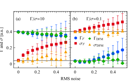
Figure 6: RMS noise test. (a) Extracted fit results $\Gamma_{F},\sigma_{F}$ for $\Gamma/\sigma=10$ under RMS noise with the FLA method and direct least-squares fit ($\Gamma_{\mathrm{DFM}},\sigma_{\mathrm{DFM}}$). Gridlines denote the initial values before RMS noise application (b) Same as (a) with inverse contribution ratio $\Gamma/\sigma=0.1$

Funding

Swiss National Science Foundation, Grant No. 200021_166271.

Disclosures

The authors declare that they have no competing interests.

References

- van de Hulst and Reesinck [1947] H. C. van de Hulst and J. J. M. Reesinck, Line Breadths and Voigt Profiles., Astrophysical Journal 106, 121 (1947).
- Galatry [1961] L. Galatry, Simultaneous effect of doppler and foreign gas broadening on spectral lines, Phys. Rev. 122, 1218 (1961).
- Rautian and Sobel’man [1967] S. G. Rautian and I. I. Sobel’man, The effect of collisions on the doppler broadening of spectral lines, Soviet Physics Uspekhi 9, 701 (1967).
- Stokes [1948] A. R. Stokes, A numerical fourier-analysis method for the correction of widths and shapes of lines on x-ray powder photographs, Proceedings of the Physical Society 61, 382 (1948).
- WILSON [1962] A. J. C. WILSON, Variance as a measure of line broadening, Nature 193, 568 (1962).
- De Keijser et al. [1982] T. H. De Keijser, J. I. Langford, E. J. Mittemeijer, and A. B. P. Vogels, Use of the voigt function in a single-line method for the analysis of x-ray diffraction line broadening, Journal of Applied Crystallography 15, 308 (1982).
- Maletta et al. [1982] H. Maletta, G. Aeppli, and S. M. Shapiro, Spin correlations in nearly ferromagnetic , Phys. Rev. Lett. 48, 1490 (1982).
- Dirac and Bohr [1927] P. A. M. Dirac and N. H. D. Bohr, The quantum theory of the emission and absorption of radiation, Proceedings of the Royal Society of London. Series A, Containing Papers of a Mathematical and Physical Character 114, 243 (1927).
- Schober [1933] H. Schober, M. born, optik, Monatshefte für Mathematik und Physik 40, A36 (1933).
- Orear and Fermi [1967] J. Orear and E. Fermi, Nuclear physics: a course given by Enrico Fermi at the University of Chicago. (University of Chicago Press, 1967) pp. ix, 248 p., ix, 248 p.
- Enzo et al. [1988] S. Enzo, G. Fagherazzi, A. Benedetti, and S. Polizzi, A profile-fitting procedure for analysis of broadened x-ray diffraction peaks. i. methodology, Journal of Applied Crystallography 21, 536 (1988).
- Hutchinson [2002] I. H. Hutchinson, Principles of Plasma Diagnostics, 2nd ed. (Cambridge University Press, 2002).
- McLean et al. [1994] A. McLean, C. Mitchell, and D. Swanston, Implementation of an efficient analytical approximation to the voigt function for photoemission lineshape analysis, Journal of Electron Spectroscopy and Related Phenomena 69, 125 (1994).
- Liu et al. [2001] Y. Liu, J. Lin, G. Huang, Y. Guo, and C. Duan, Simple empirical analytical approximation to the voigt profile, J. Opt. Soc. Am. B 18, 666 (2001).
- Shin [2014] B.-k. Shin, A simple quasi-analytical method for the deconvolution of voigtian profiles, Journal of Magnetic Resonance 249, 1 (2014).
- Matmon et al. [2016] G. Matmon, S. A. Lynch, T. F. Rosenbaum, A. J. Fisher, and G. Aeppli, Optical response from terahertz to visible light of electronuclear transitions in , Phys. Rev. B 94, 205132 (2016).
- Planck [1917] M. Planck, Zur theorie des rotationsspektrums, Annalen der Physik 357, 491 (1917).
- Jung et al. [1931] G. Jung, H. Gude, and G. Jung, Das rotationsschwingungsspektrum des gasförmigen, flüssigen und gelösten ammoniaks, Zeitschrift für Elektrochemie und angewandte physikalische Chemie 37, 545 (1931).
- Albert et al. [2011a] S. Albert, K. K. Albert, and M. Quack, High-resolution fourier transform infrared spectroscopy, in Handbook of High-resolution Spectroscopy (American Cancer Society, 2011) https://onlinelibrary.wiley.com/doi/pdf/10.1002/9780470749593.hrs042 .
- Ruland [1968] W. Ruland, The separation of line broadening effects by means of line-width relations, Journal of Applied Crystallography 1, 90 (1968).
- Klein and Furtak [1986] M. V. Klein and T. E. Furtak, Optics (Wiley, New York, 1986).
- Olivero and Longbothum [1977] J. Olivero and R. Longbothum, Empirical fits to the voigt line width: A brief review, Journal of Quantitative Spectroscopy and Radiative Transfer 17, 233 (1977).
- Albert et al. [2011b] S. Albert, K. K. Albert, P. Lerch, and M. Quack, Synchrotron-based highest resolution fourier transform infrared spectroscopy of naphthalene (c10h8) and indole (c8h7n) and its application to astrophysical problems, Faraday Discuss. 150, 71 (2011b).
- Als-Nielsen and McMorrow [2011] J. Als-Nielsen and D. McMorrow, Kinematical scattering ii: crystalline order, in Elements of Modern X-ray Physics (John Wiley & Sons, Ltd, 2011) Chap. 5, pp. 147–205, https://onlinelibrary.wiley.com/doi/pdf/10.1002/9781119998365.ch5 .
- Holler et al. [2017] M. Holler, M. Guizar-Sicairos, E. H. R. Tsai, R. Dinapoli, E. Müller, O. Bunk, J. Raabe, and G. Aeppli, High-resolution non-destructive three-dimensional imaging of integrated circuits, Nature 543, 402 (2017).
- Holler et al. [2019] M. Holler, M. Odstrcil, M. Guizar-Sicairos, M. Lebugle, E. Müller, S. Finizio, G. Tinti, C. David, J. Zusman, W. Unglaub, O. Bunk, J. Raabe, A. F. J. Levi, and G. Aeppli, Three-dimensional imaging of integrated circuits with macro- to nanoscale zoom, Nature Electronics 2, 464 (2019).
- Hänsch [2005] T. W. Hänsch, Passion for precision (2005).
- Harris [1978] F. J. Harris, On the use of windows for harmonic analysis with the discrete fourier transform, Proceedings of the IEEE 66, 51 (1978).
- Nuttall [1981] A. Nuttall, Some windows with very good sidelobe behavior, IEEE Transactions on Acoustics, Speech, and Signal Processing 29, 84 (1981).