\NewBibliographyString

toappear

11institutetext: Fraunhofer Center for Machine Learning 22institutetext: Fraunhofer-Institut für Techno- und Wirtschaftsmathematik ITWM, Fraunhofer-Platz 1, 67663 Kaiserslautern, Germany 33institutetext: Fraunhofer-Institut für Werkstoffmechanik IWM, Wöhlerstr. 11, 79108 Freiburg, Germany

CupNet – Pruning a network for geometric data

Raoul Heese 1122 raoul.heese@itwm.fraunhofer.de 0000-0001-7479-3339    Lukas Morand 33 0000-0002-8566-7642    Dirk Helm 33 0000-0002-5398-5443    Michael Bortz 1122 0000-0001-8169-2907
Abstract

Using data from a simulated cup drawing process, we demonstrate how the inherent geometrical structure of cup meshes can be used to effectively prune an artificial neural network in a straightforward way.

Keywords:
regression, informed learning, pruning, network architecture, deep drawing

1 Introduction

The optimization of production processes can benefit from machine learning methods that incorporate domain knowledge and data from numerical simulations [1]. Typically, such methods aim to model relations between process parameters and the resulting product. In this manuscript, we consider an example from the field of deep drawing, a sheet metal forming process in which a sheet metal blank is drawn into a forming die by mechanical action.

Specifically, we study the prediction of product geometries in a cup drawing process based on data from finite element simulations [2]. For each simulation, we choose randomized process and material parameters 𝐩k𝐩superscript𝑘\mathbf{p}\in\mathbb{R}^{k} with k9𝑘9k\equiv$9$ and observe the resulting geometry as a set of m1 979𝑚1979m\equiv$1\,979$ mesh coordinates 𝐱d𝐱superscript𝑑\mathbf{x}\in\mathbb{R}^{d} with d3m=5 937𝑑3𝑚5937d\equiv 3m=$5\,937$. Thus, the machine learning task is to predict

$\displaystyle\mathbf{\hat{x}}(\mathbf{p}):\mathbb{R}^{k}\longmapsto\mathbb{R}^{d}$ (1)

based on the generated data. Such a predictive regression model can be considered as a short-cut for the actual simulation. In contrast to the simulation, it is faster and always numerically stable and therefore particularly suitable to solve optimization problems. On the other hand, the model predictions are less accurate than the simulation results, which corresponds to a trade-off between calculation speed and outcome precision.

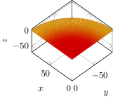
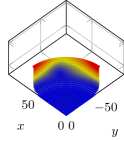
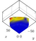
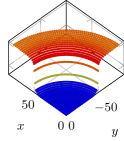
The choice of parameters affects the resulting cup quality in the sense that we can infer good, defect and cracked cups (indicated by strong deformations) from the mesh geometries. In total, we ran $10\,000$ simulations, of which two failed (for numerical reasons). Of the remaining $9\,998$ parameter combinations, $3\,991$ lead to good cups, $5\,075$ lead to defect cups and $932$ cause cracked cups, cf. Fig. 1.

Refer to caption
a) Before deformation.
Refer to caption
b) Good cup.
Refer to caption
c) Defect cup.
Refer to caption
d) Cracked cup.
Figure 1: Typical cup geometries, each consisting of $m$ points. For reasons of symmetry, it is sufficient to simulate the deformation of a quarter cup segment instead of the full cup. The colors indicate the distance of each point to the reference mesh, consisting of the average coordinates of all good cups. We use a different color scale for each subfigure: 0            1a) 70, 1b) 2, 1c) 6, 1d) 49.

2 Method

We propose two artificial neural networks to model Eq. 1. Our first network architecture, which we call CupNet, particularly takes the geometrical structure of the data into account to effectively prune the network weights. Pruning is a technique that helps in the development of smaller and more efficient networks, see, e. g., Refs. [3, 4] and references therein. That means, instead of changing the loss function as in e. g., Ref. [5], we use expert knowledge to change the network architecture itself.

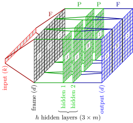
The proposed network consists of an input layer of size $k$ (i. e., it contains $k$ units), which is fully connected to an initial layer of size $d$, which we call frame. We split the frame layer into three evenly sized segments (i. e., one for each dimension denoted by $x$, $y$, and $z$, cf. Fig. 1), which are each connected to the following layers in a special way. Specifically, we chose the forward pass

$\displaystyle\mathbf{o}\equiv A([\mathbf{C}(\alpha)\odot\mathbf{W}]^{\intercal}\mathbf{i}+\mathbf{b}).$ (2)

Here $\mathbf{i}\in\mathbb{R}^{m\times 1}$ and $\mathbf{o}\in\mathbb{R}^{m\times 1}$ represent the layer inputs and outputs, whereas $\mathbf{W}\in\mathbb{R}^{m\times m}$ and $\mathbf{b}\in\mathbb{R}^{m\times 1}$ stand for the (trainable) layer weights and biases, and $A(\cdot)$ represents the activation function. The symbol $\odot$ denotes the Hadamard product (element-wise multiplication). Moreover, we have introduced the symmetric pruning matrix $\mathbf{C}(\alpha)\in\{0,1\}^{m\times m}$ with elements

$\displaystyle\mathbf{C}_{ij}(\alpha)\equiv\begin{cases}0&\text{if}\,\,\mathbf{D}_{ij}>\alpha\\ 1&\text{if}\,\,\mathbf{D}_{ij}\leq\alpha\end{cases}\hskip 24.18501pt\text{with}\hskip 24.18501pt\mathbf{D}_{ij}\equiv||\mathbf{x^{\prime}_{i}}-\mathbf{x^{\prime}_{j}}||_{2}=\operatorname{const.}$ (3)

for $i,j=1,\dots,m$. It is based on the symmetric distance matrix $\mathbf{D}\in\mathbb{R}_{\geq 0}^{m\times m}$, which contains the euclidean distances $||\cdot||_{2}$ between different mesh points $\mathbf{x^{\prime}}$ of the undeformed geometry, Fig. 1a). Thus, the pruning matrix removes the influence of all weights for which the corresponding mesh points of the undeformed geometry have a distance beyond the user-defined pruning threshold $\alpha\geq 0$.

This special layer configuration is repeated $h$ times and concludes with a fully-connected last layer merging the three previously splitted segments into the output layer. Summarized, we use the inherent geometrical structure of the data to prune a fully connected network in such a way that correlations between spatially related mesh points are preserved. The complete architecture is sketched in Fig. 2a).

Refer to caption
a) Our proposed CupNet with $n_{\mathrm{cup}}(h,\alpha)$ trainable parameters, Eq. 4, and dimensions $x$, $y$, and $z$.
Refer to caption
b) The reference network RefNet with $n_{\mathrm{ref}}(h,s)$ trainable parameters, Eq. 5.
Figure 2: Network architectures used to model Eq. 1. The $k$-dimensional simulation parameters $\color[rgb]{.8,.0,.0}\definecolor[named]{pgfstrokecolor}{rgb}{.8,.0,.0}\mathbf{p}$ constitute the input, whereas the output corresponds to the $d$-dimensional mesh ${\color[rgb]{.0,.0,.8}\definecolor[named]{pgfstrokecolor}{rgb}{.0,.0,.8}\mathbf{\hat{x}}}({\color[rgb]{.8,.0,.0}\definecolor[named]{pgfstrokecolor}{rgb}{.8,.0,.0}\mathbf{p}})$. Both architectures consist of a sequence of layers (number of units in brackets), which are fully connected (F) or partially connected, i. e., pruned (P). We apply a dropout after every inner layer for regularization.

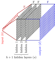
As a reference we also use a second architecture, which we call RefNet. It has a similar structure and complexity as the CupNet, but does not take advantage of the geometrical structure of the data. Specifically, it consists of an input layer of size $k$, $h+1$ hidden layers of size $s$ and an output layer of size $m$, all of which are fully connected. In order to obtain a comparable complexity of the two architectures we choose $s$ in such a way that the number of trainable parameters is as close as possible. For that, we first determine the number of trainable parameters for the CupNet architecture

$\displaystyle n_{\mathrm{cup}}(h,\alpha)=(k\cdot d+d)+3h(c(\alpha)+m)+3(m^{2}+m)\hskip 24.18501pt\text{with}\hskip 24.18501ptc(\alpha)\equiv\sum_{i,j=1}^{m}\mathbf{C}_{ij}(\alpha).$ (4)

On the other hand, the number of trainable parameters for the RefNet architecture reads

$\displaystyle n_{\mathrm{ref}}(h,s)=(k\cdot s+s)+h(s^{2}+s)+(s\cdot d+d)$ (5)

so that the condition $n_{\mathrm{ref}}(h,s)\overset{!}{=}n_{\mathrm{cup}}(h,\alpha)$ leads to $s(h,\alpha)=(-u+\sqrt{u^{2}-4h(d-n_{\mathrm{cup}}(h,\alpha))})/(2h)$, where $u\equiv k+h+d+1$. We set the layer size $s$ to the ceiling of this value for a given depth $h$ and a given pruning threshold $\alpha$. The complete RefNet architecture is sketched in Fig. 2b).

For both networks the activation function is chosen to be a ReLU for all but the output layer for which we use a linear activation. As a regularizer we apply a dropout after every inner layer, where we randomly set 20%percent20$20$\% of the units to zero.

3 Experiments

We test the performance of both network architectures, which we have implemented using Ref. [6]. For this purpose we split the standardized data into a training set with $9\,000$ elements and a test set with $998$ elements stratified according to the three cup classes of good cups, defect cups, and cracked cups. We repeat this approach for $10$ benchmark runs with different data splittings and different random seeds for the network initialization. For the training we use an Adam optimizer and a mean squared error for the loss. As a result, we obtain the $R^{2}$ scores shown in Table 1.

Table 1: $R^{2}$ score means and standard deviations over all 10 benchmark runs for different values of the network depth $h$ and the pruning threshold $\alpha$. The best mean results are highlighted in colored bold.
network α=1.0𝛼1.0\alpha=$1.0$ α=2.5𝛼2.5\alpha=$2.5$ α=5.0𝛼5.0\alpha=$5.0$ α=10.0𝛼10.0\alpha=$10.0$ α=25.0𝛼25.0\alpha=$25.0$ α=50.0𝛼50.0\alpha=$50.0$
CupNet (h=1)1(h=$1$) 0.822±0.042uncertain0.8220.0420.822\pm 0.042 0.823±0.052uncertain0.8230.0520.823\pm 0.052 0.829±0.040uncertain0.8290.0400.829\pm 0.040 0.832±0.084uncertain0.8320.0840.832\pm 0.084 0.839±0.044uncertain0.8390.0440.839\pm 0.044 0.819±0.072uncertain0.8190.0720.819\pm 0.072
RefNet (h=1)1(h=$1$) 0.818±0.047uncertain0.8180.0470.818\pm 0.047 0.818±0.066uncertain0.8180.0660.818\pm 0.066 0.815±0.066uncertain0.8150.0660.815\pm 0.066 0.817±0.045uncertain0.8170.0450.817\pm 0.045 0.818±0.056uncertain0.8180.0560.818\pm 0.056 0.817±0.053uncertain0.8170.0530.817\pm 0.053
CupNet (h=2)2(h=$2$) 0.821±0.038uncertain0.8210.0380.821\pm 0.038 0.850±0.039uncertain0.8500.0390.850\pm 0.039 0.862±0.046uncertain0.8620.0460.862\pm 0.046 0.851±0.057uncertain0.8510.0570.851\pm 0.057 0.847±0.047uncertain0.8470.0470.847\pm 0.047 0.831±0.045uncertain0.8310.0450.831\pm 0.045
RefNet (h=2)2(h=$2$) 0.804±0.050uncertain0.8040.0500.804\pm 0.050 0.813±0.061uncertain0.8130.0610.813\pm 0.061 0.809±0.048uncertain0.8090.0480.809\pm 0.048 0.821±0.036uncertain0.8210.0360.821\pm 0.036 0.803±0.037uncertain0.8030.0370.803\pm 0.037 0.800±0.070uncertain0.8000.0700.800\pm 0.070
CupNet (h=3)3(h=$3$) 0.830±0.039uncertain0.8300.0390.830\pm 0.039 0.849±0.039uncertain0.8490.0390.849\pm 0.039 0.850±0.053uncertain0.8500.0530.850\pm 0.053 0.861±0.056uncertain0.8610.0560.861\pm 0.056 0.839±0.053uncertain0.8390.0530.839\pm 0.053 0.829±0.043uncertain0.8290.0430.829\pm 0.043
RefNet (h=3)3(h=$3$) 0.811±0.043uncertain0.8110.0430.811\pm 0.043 0.789±0.085uncertain0.7890.0850.789\pm 0.085 0.826±0.042uncertain0.8260.0420.826\pm 0.042 0.802±0.064uncertain0.8020.0640.802\pm 0.064 0.810±0.045uncertain0.8100.0450.810\pm 0.045 0.827±0.029uncertain0.8270.0290.827\pm 0.029
CupNet (h=4)4(h=$4$) 0.830±0.040uncertain0.8300.0400.830\pm 0.040 0.838±0.050uncertain0.8380.0500.838\pm 0.050 0.845±0.064uncertain0.8450.0640.845\pm 0.064 0.849±0.035uncertain0.8490.0350.849\pm 0.035 0.817±0.114uncertain0.8170.1140.817\pm 0.114 0.806±0.034uncertain0.8060.0340.806\pm 0.034
RefNet (h=4)4(h=$4$) 0.797±0.055uncertain0.7970.0550.797\pm 0.055 0.792±0.044uncertain0.7920.0440.792\pm 0.044 0.800±0.052uncertain0.8000.0520.800\pm 0.052 0.808±0.041uncertain0.8080.0410.808\pm 0.041 0.779±0.051uncertain0.7790.0510.779\pm 0.051 0.768±0.068uncertain0.7680.0680.768\pm 0.068
CupNet (h=5)5(h=$5$) 0.478±0.292uncertain0.4780.2920.478\pm 0.292 0.835±0.064uncertain0.8350.0640.835\pm 0.064 0.838±0.048uncertain0.8380.0480.838\pm 0.048 0.839±0.037uncertain0.8390.0370.839\pm 0.037 0.832±0.036uncertain0.8320.0360.832\pm 0.036 0.805±0.033uncertain0.8050.0330.805\pm 0.033
RefNet (h=5)5(h=$5$) 0.762±0.060uncertain0.7620.0600.762\pm 0.060 0.774±0.041uncertain0.7740.0410.774\pm 0.041 0.789±0.038uncertain0.7890.0380.789\pm 0.038 0.767±0.050uncertain0.7670.0500.767\pm 0.050 0.778±0.042uncertain0.7780.0420.778\pm 0.042 0.691±0.126uncertain0.6910.1260.691\pm 0.126
CupNet (h=6)6(h=$6$) 0.052±0.108uncertain0.0520.1080.052\pm 0.108 0.832±0.042uncertain0.8320.0420.832\pm 0.042 0.840±0.046uncertain0.8400.0460.840\pm 0.046 0.832±0.103uncertain0.8320.1030.832\pm 0.103 0.832±0.045uncertain0.8320.0450.832\pm 0.045 0.787±0.080uncertain0.7870.0800.787\pm 0.080
RefNet (h=6)6(h=$6$) 0.780±0.041uncertain0.7800.0410.780\pm 0.041 0.785±0.039uncertain0.7850.0390.785\pm 0.039 0.769±0.049uncertain0.7690.0490.769\pm 0.049 0.770±0.045uncertain0.7700.0450.770\pm 0.045 0.765±0.019uncertain0.7650.0190.765\pm 0.019 0.436±0.129uncertain0.4360.1290.436\pm 0.129
CupNet (h=7)7(h=$7$) 0.053±0.161uncertain0.0530.1610.053\pm 0.161 0.714±0.191uncertain0.7140.1910.714\pm 0.191 0.843±0.049uncertain0.8430.0490.843\pm 0.049 0.857±0.033uncertain0.8570.0330.857\pm 0.033 0.825±0.051uncertain0.8250.0510.825\pm 0.051 0.781±0.049uncertain0.7810.0490.781\pm 0.049
RefNet (h=7)7(h=$7$) 0.772±0.034uncertain0.7720.0340.772\pm 0.034 0.761±0.058uncertain0.7610.0580.761\pm 0.058 0.755±0.040uncertain0.7550.0400.755\pm 0.040 0.755±0.031uncertain0.7550.0310.755\pm 0.031 0.592±0.243uncertain0.5920.2430.592\pm 0.243 0.377±0.203uncertain0.3770.2030.377\pm 0.203

We find that in most cases, CupNet is superior to RefNet. It performs worse only for low α𝛼\alpha and large hh (i. e., strong pruning and deep nets). In these cases, the training process appears to not converge to a sufficiently good state. However, the mean scores of the two architectures are mostly within one standard deviation of each other. The best mean CupNet score of 0.8620.8620.862 is achieved for h=22h=$2$ and α=5𝛼5\alpha=$5$, which corresponds to a network with ncup=12 277 950subscript𝑛cup12277950n_{\mathrm{cup}}=$12\,277\,950$ trainable parameters. On the other hand, the best mean RefNet score of 0.8270.8270.827 is achieved for h=33h=$3$ and α=50𝛼50\alpha=$50$, which corresponds to a much larger network with nref=34 898 737subscript𝑛ref34898737n_{\mathrm{ref}}=$34\,898\,737$ trainable parameters. Thus, according to the respective optimal values for hh and α𝛼\alpha, our pruning approach leads to smaller networks with a better expected score.

As an alternative approach we also test the performance of a Random Forest regressor (with 250 trees) on PCA-transformed features (with 100 components) using the implementation from Ref. [7]. This leads to a $R^{2}$ score of $0.736\pm 0.029$ over 10 benchmark runs, which is worse than most results from Table 1.

4 Conclusion

Summarized, our approach of pruning the network connections according to the spatial correlation of mesh points leads to a better expected performance in comparison with a reference network with similar structure and complexity for our specific use case. A more detailed analysis of this observation is beyond the scope of this paper. However, testing whether our approach can also be applied to other geometrical data could serve as a possible starting point for further research.

5 Acknowledgements

We would like to thank Alexander Butz for helpful discussions, Maria Baiker and Jan Pagenkopf for providing the simulation of the cup drawing process, and Boris Giba for data processing. This work was developed in the Fraunhofer Cluster of Excellence “Cognitive Internet Technologies” as well as the Fraunhofer lighthouse project “Machine Learning for Production”.

References

  • [1] Laura Rueden et al. “Informed Machine Learning – A Taxonomy and Survey of Integrating Prior Knowledge into Learning Systems” In IEEE Transactions on Knowledge and Data Engineering Institute of ElectricalElectronics Engineers (IEEE), 2021 DOI: 10.1109/tkde.2021.3079836
  • [2] L Morand, D Helm, R Iza-Teran and J Garcke “A knowledge-based surrogate modeling approach for cup drawing with limited data” In IOP Conference Series: Materials Science and Engineering 651 IOP Publishing, 2019, pp. 012047 DOI: 10.1088/1757-899x/651/1/012047
  • [3] Zhuang Liu et al. “Rethinking the Value of Network Pruning”, 2019 arXiv:1810.05270 [cs.LG]
  • [4] Davis Blalock, Jose Javier Gonzalez Ortiz, Jonathan Frankle and John Guttag “What is the State of Neural Network Pruning?”, 2020 arXiv:2003.03033 [cs.LG]
  • [5] Raoul Heese et al. “The Good, the Bad and the Ugly: Augmenting a Black-Box Model with Expert Knowledge” In Artificial Neural Networks and Machine Learning – ICANN 2019: Workshop and Special Sessions Springer, 2019, pp. 391–395
  • [6] Martín Abadi et al. “TensorFlow: Large-Scale Machine Learning on Heterogeneous Systems”, 2015
  • [7] F. Pedregosa et al. “Scikit-learn: Machine Learning in Python” In Journal of Machine Learning Research 12, 2011, pp. 2825–2830