1 Introduction

Federated learning is a rapidly evolving application of distributed optimization for estimation and learning problems in large-scale networks of remote clients [13]. These systems present new challenges, as they are characterized by heterogeneity in computational resources and data across the network, unreliable communication, massive scale, and privacy constraints [16]. A typical application is for developers of cell phones and cellular applications to model the usage of software and devices across millions or even billions of users.

Distributed optimization has a rich history and extensive literature (e.g., see the sources [2, 5, 8, 31, 15, 24] and references therein), and federated learning has led to a flurry of interest in the area. A number of different procedures have been proposed for federated learning and related problems, using methods based on stochastic gradient methods or proximal procedures. Notably, McMahan et al. [18] introduced the FedSGD and FedAvg algorithms, which both adapt the classical stochastic gradient method to the federated setting, considering the possibility that clients may fail and may only be subsampled on each round of computation. Another recent proposal has been to use regularized local problems to mitigate possible issues that arise with device heterogeneity and failures [17]. These authors propose the FedProx procedure, an algorithm that applied averaged proximal updates to solve federated minimization problems.

Currently, the convergence theory and correctness of these methods is currently lacking, and practitioners have documented failures of convergence in certain settings (e.g., see Figure 3 and related discussion in the work [18]). Our first contribution in this paper is to analyze the deterministic analogues of these procedures, in which the gradient or proximal updates are performed using the full data at each client; such updates can be viewed as the idealized limit of a minibatch update based on the entire local dataset. Even in this especially favorable setting, we show that most versions of these algorithms fail to preserve the fixed points of the original optimization problem: that is, even if they converge, the resulting fixed points need not be stationary. Since the stochastic updates implemented in current practice are randomized versions of the underlying deterministic procedures, they also fail to preserve the correct fixed points in general.

In order to address this issue, we show how operator splitting techniques [5, 28, 7, 1] can be exploited to permit the development of provably correct and convergence procedures for solving federated problems. Concretely, we propose a new family of federated optimization algorithms, that we refer to as FedSplit. These procedures us to solve distributed convex minimization problems of the form

$$\text{minimize}\quad F(x)\mathrel{\hbox to0.0pt{\raisebox{1.29167pt}{$\cdot$}\hss}\raisebox{-1.29167pt}{$\cdot$}}=\sum_{j=1}^{m}f_{j}(x),$$ (1)

where $f_{j}\colon\mathbf{R}^{d}\to\mathbf{R}$ are cost functions that each client assigns to the optimization variable $x\in\mathbf{R}^{d}$. In machine learning applications, the vector $x\in{}^{d}$ is a parameter of a statistical model. In this paper, we focus on the case when $f_{j}$ are finite convex functions, with Lipschitz continuous gradient. While such problems are pervasive in data fitting applications, this necessarily precludes the immediate application of our methods and guarantees to constrained, nonsmooth, and nonconvex problems. We leave the analysis and development of such methods to future work.

As previously mentioned, distributed optimization is not a new discipline, with work dating back to the 1970s and 1980s [2]. Over the past decade, there has been a resurgence of research on distributed optimization, specifically for learning problems [5, 8, 31, 15, 24]. This line of work builds upon even earlier study of distributed first- and second-order methods designed for optimization in the “data center” setting [2]. In these applications, the devices that carry out the computation are high performance computing clusters with computational resources that are well-known. This is in contrast to the federated setting, where the clients that carry out computation are cell phones or other computationally-constrained mobile devices for which carrying out expensive, exact computations of intermediate quantities may be unrealistic. Therefore, it is important to have methods that permit approximate computation, with varying levels of accuracy throughout the network of participating agents [4].

Our development makes use of a long line of work that adapts the theory of operator-splitting methods to distributed optimization [5, 28, 7, 1]. In particular, the FedSplit procedure developed in this paper is based upon an application of the Peaceman-Rachford splitting [21] to the distributed convex problem (1). This method and its variants have been studied extensively in the general setting of root-finding for the sum of two maximally monotone operators. Recent works have studied such splitting schemes for convex minimization under strong convexity and smoothness assumptions [11, 10, 19]. In this paper, we adapt this general theory to the specific setting of federated learning, and extend it to apply beyond strongly convex losses. Furthermore, we extend this previous work to the setting when specific intermediate quantities—likely to dominate the computational cost of on-device training—are inexact and cheaply computed.

The remainder of this paper is organized as follows. We begin with a discussion of two previously proposed methods for solving federated optimization problems in Section 2. We show that these methods cannot have a generally applicable convergence theory as these methods have fixed points that are not solutions to the federated optimization problems they are designed to solve. In Section 3, we present the FedSplit procedure, and demonstrate that, unlike some other methods in use, it has fixed points that do correspond to optimal solutions of the original federated optimization problem. After presenting convergence results, we present numerical experiments in Section 4. These experiments confirm our theoretical predictions and also demonstrate that our methods enjoy favorable scaling in the problem conditioning. Section 5 is devoted to the proofs of our results. We conclude in Section 6 with future directions suggested by the development in this paper.

1.1 Notation

For the reader’s convenience, we collect here our notational conventions.

Set and vector arithmetic:

Given vectors $x,y\in{}^{d}$, we use $x^{\mathsf{T}}y=\sum_{j=1}^{d}x_{j}y_{j}$ to denote their Euclidean inner product, and $\|x\|=\sqrt{x^{\mathsf{T}}x}$ to denote the Euclidean norm. Given two non-empty subsets $A,B\subset\mathbf{R}^{d}$, their Minkowski sum is given by $A+B=\{x+y\mid x\in A,y\in B\}$. We also set $x+B=\{x\}+B$ for any point $x\in\mathbf{R}^{d}$.

For an integer $m\geqslant 1$, we use the shorthand $[m]\mathrel{\hbox to0.0pt{\raisebox{1.29167pt}{$\cdot$}\hss}\raisebox{-1.29167pt}{$\cdot$}}=\{1,\ldots,m\}$. Given a block-partitioned vector $z=(z_{1},\dots,z_{m})\in({}^{d})^{m}$ with $z_{j}\in\mathbf{R}^{d}$ for $j\in[m]$, we define the block averaged vector $\overline{z}\mathrel{\hbox to0.0pt{\raisebox{1.29167pt}{$\cdot$}\hss}\raisebox{-1.29167pt}{$\cdot$}}=\frac{1}{m}\sum_{j=1}^{m}z_{j}$. Very occasionally, we also slightly abuse notation by defining arithmetic between vectors of dimension with a common factor. For example, if $x\in\mathbf{R}^{d}$ and $(y_{1},\dots,y_{m})=y\in(\mathbf{R}^{d})^{m}$, then

$$x+y\mathrel{\hbox to0.0pt{\raisebox{1.29167pt}{$\cdot$}\hss}\raisebox{-1.29167pt}{$\cdot$}}=(x+y_{1},\dots,x+y_{m}).$$

Regularity conditions:

A differentiable function $f\colon\mathbf{R}^{d}\to\mathbf{R}$ is said to be $\ell$-strongly convex if

$$f(y) \geqslant f(x)+\nabla f(x)^{\mathsf{T}}(y-x)+\frac{\ell}{2}\|y-x\|^{2},\quad\text{for all}\quad x,y\in\mathbf{R}^{d}.$$

It is simply convex if this condition holds with $\ell=0$. Similarly, a differentiable function $f\colon\mathbf{R}^{d}\to\mathbf{R}$ is $L$-smooth if its gradient $\nabla f$ is $L$-Lipschitz continuous,

$$\|\nabla f(x)-\nabla f(y)\|\leqslant L\|x-y\|,\quad\text{for all}~{}x,y\in\mathbf{R}^{d}.$$

Operator notation:

Given an operator $\mathcal{T}\colon\mathbf{R}^{d}\to\mathbf{R}^{d}$ and a positive integer $k$, we use $\mathcal{T}^{k}$ to denote the composition of $\mathcal{T}$ with itself $k$ times—that is, $\mathcal{T}^{k}$ is a new operator that acts on a given $x\in{}^{d}$ as $\mathcal{T}^{k}x\mathrel{\hbox to0.0pt{\raisebox{1.29167pt}{$\cdot$}\hss}\raisebox{-1.29167pt}{$\cdot$}}=\underbrace{\mathcal{T}\circ\mathcal{T}\circ\cdots\circ\mathcal{T}}_{k~{}\text{times}}x$. An operator $\mathcal{T}\colon\mathbf{R}^{d}\to\mathbf{R}^{d}$ is said to be monotone if

$$\left(\mathcal{T}y-\mathcal{T}x\right)^{\mathsf{T}\!}(y-x)\geqslant 0\qquad\mbox{for all $x,y\in{}^{d}$.}$$ (2)

2 Existing algorithms and their fixed points

Prior to proposing our own algorithms, let us discuss the fixed points of the deterministic analogues of some methods recently proposed for federated optimization problems (1). We focus our discussion on two recently proposed procedures—namely, FedSGD [18] and FedProx [17].

In understanding these and other algorithms, it is convenient to introduce the consensus reformulation of the distributed problem (1), which takes the form

$$\begin{array}[]{ll}\text{minimize}&F(x)\mathrel{\hbox to0.0pt{\raisebox{1.29167pt}{$\cdot$}\hss}\raisebox{-1.29167pt}{$\cdot$}}=\sum_{j=1}^{m}f_{j}(x_{j})\\ \text{subject to}&x_{1}=x_{2}=\cdots=x_{m}.\end{array}$$ (5)

Although this consensus formulation involves more variables, it is more amenable to the analysis of distributed procedures [5].

2.1 Federated gradient algorithms

The recently proposed FedSGD method [18] is based on a multi-step projected stochastic gradient method for solving the consensus problem. Given the iterates $\{x_{j}^{(t)},j=1,\ldots,m\}$ at iteration $t$, the method is based on taking some number $e\geqslant 1$ of stochastic gradient steps with respect to each loss $f_{j}$, and then passing to the coordinating agent to compute an average, which yields the next iterate in the sequence. When a single stochastic gradient step ($e=1$) is taken between the averaging steps, this method can be seen as a variant of projected stochastic gradient descent for the consensus problem (5) and by classical theory of convex optimization enjoys convergence guarantees [14]. On the other hand, when the number of epochs $e$ is strictly larger than 1, it is unclear a priori if the method should retain the same guarantees.

As we discuss here, even without the additional inaccuracies introduced by using stochastic approximations to the local gradients, FedSGD with $e>1$ will not converge to minima in general. More precisely, let us consider the deterministic version of this method (which can be thought of the ideal case that would be obtained when the mini-batches at each device are taken to infinity). Given a stepsize $s>0$, define the gradient mappings

$$G_{j}(x)\mathrel{\hbox to0.0pt{\raisebox{1.29167pt}{$\cdot$}\hss}\raisebox{-1.29167pt}{$\cdot$}}=x-s\nabla f_{j}(x)\qquad\mbox{ for $j=1,\dots,m$.}$$ (6)

For a given integer $e\geqslant 1$, we define the $e$-fold composition

$$G_{j}^{e}(x) \mathrel{\hbox to0.0pt{\raisebox{1.29167pt}{$\cdot$}\hss}\raisebox{-1.29167pt}{$\cdot$}}=\underbrace{\big{(}G_{j}\circ G_{j}\circ\ldots\circ G_{j}\big{)}}_{\mbox{$e$-times}}(x)\qquad\mbox{for all $x\in{}^{d}$,}$$ (7)

corresponding to taking $e$ gradient steps from a given point $x$. We also define $G_{j}^{0}$ to be the identity operator—that is, $G_{j}^{0}(x)\mathrel{\hbox to0.0pt{\raisebox{1.29167pt}{$\cdot$}\hss}\raisebox{-1.29167pt}{$\cdot$}}=x$ for all $x\in{}^{d}$.

In terms of these operators, we can define a family of FedGD$(s,e)$ algorithms, with each algorithm parameterized by a choice of stepsize $s>0$ and number of gradient rounds $e\geqslant 1$. Given an initialization $x^{(1)}$, it performs the following updates for $t=1,2,\ldots$:

$$x_{j}^{(t+1/2)} \mathrel{\hbox to0.0pt{\raisebox{1.29167pt}{$\cdot$}\hss}\raisebox{-1.29167pt}{$\cdot$}}=G_{j}^{e}(x_{j}^{(t)}), j\in[m]\mathrel{\hbox to0.0pt{\raisebox{1.29167pt}{$\cdot$}\hss}\raisebox{-1.29167pt}{$\cdot$}}=\{1,2,\dots,m\}$$ for , and (8a)

$$x_{j}^{(t+1)} \mathrel{\hbox to0.0pt{\raisebox{1.29167pt}{$\cdot$}\hss}\raisebox{-1.29167pt}{$\cdot$}}=\overline{x}^{(t+1/2)}, j\in[m]$$ for , (8b)

where the reader should recall that $\overline{x}^{(t+1/2)}=\tfrac{1}{m}\sum_{j=1}^{m}x_{j}^{(t+1/2)}$ is the block average.

Proposition 1.

For any $s>0$ and $e\geqslant 1$, the sequence $\{x^{(t)}\}_{t=1}^{\infty}$ generated by the FedGD$(s,e)$ algorithm in equation (8) has the following properties:

1. If $x^{(t)}$ is convergent, then the local variables $x_{j}^{(t)}$ share a common limit $x^{\star}$ such that $x_{j}^{(t)}\to x^{\star}$ as $t\to\infty$ for $j\in[m]$.

2. Moreover, the limit $x^{\star}$ satisfies the fixed point relation

   $$\sum_{i=1}^{e}\sum_{j=1}^{m}\nabla f_{j}(G_{j}^{i-1}(x^{\star}))=0.$$ (9)

See Section 5.3.1 for the proof of this claim.

Unpacking this claim slightly, suppose first that $e=1$, meaning that a single gradient update is performed at each device between the global averaging step. In this case, recalling that $G_{j}^{0}$ is the identity mapping, we have $\sum_{i=1}^{e}\nabla f_{j}(G_{j}^{i-1}(x^{\star}))=\nabla f_{j}(x^{\star})$, so that if $x^{(t)}$ has a limit $x$, it must satisfy the relations

$$x_{1}=x_{2}=\cdots=x_{m}\quad\text{and}\quad\sum_{j=1}^{m}\nabla f_{j}(x_{j})=0.$$

Consequently, provided that the losses $f_{j}$ are convex, Proposition 1 implies that the limit of the sequence $x^{(t)}$, when it exists, is a minimizer of the consensus problem (5).

On the other hand, when $e>1$, a limit of the iterate sequence $x^{(t)}$ must satisfy the equation (9), which in general causes the method to have limit points which are not minimizers of the consensus problem. For example, when $e=2$, a fixed point $x^{\star}$ satisfies the condition

$$\sum_{j=1}^{m}\left\{\nabla f_{j}(x^{\star})+\nabla f_{j}\big{(}x^{\star}-s\nabla f_{j}(x^{\star})\big{)}\right\} =0.$$

This is not equivalent to being a minimizer of the distributed problem or its consensus reformulation, in general.

It is worth noting a very special case in which FedGD will preserve the correct fixed points, even when $e>1$. In particular, suppose that all of local cost functions share a common minimizer $x^{\star}$, so that $\nabla f_{j}(x^{\star})=0$ for $j\in[m]$. Under this assumption, we have $G_{j}(x^{\star})=x^{\star}$ all $j\in[m]$, and hence by arguing inductively, we have $G_{j}^{i}(x^{\star})=x^{\star}$ for all $i\geqslant 1$. Consequently, the fixed point relation (9) reduces to

$$\sum_{i=1}^{e}\sum_{j=1}^{m}\nabla f_{j}(x^{\star})=0,$$

showing that $x^{\star}$ is optimal for the original federated problem. However, the assumption that all the local cost functions $f_{j}$ share a common optimum $x^{\star}$, either exactly or approximately, is not realistic in practice. In fact, if this assumption were to hold in practice, then there would be little point in sharing data between devices by solving the federated learning problem.

Returning to the general setting in which the fixed points need not be preserved, let us make our observation concrete by specializing the discussion to a simple class of distributed least squares problems.

Incorrectness for least squares problems:

For $j=1,\ldots,m$, suppose that we are given a design matrix $A_{j}\in\mathbf{R}^{n_{j}\times d}$ and a response vector $b_{j}\in\mathbf{R}^{n_{j}}$ associated with a linear regression problem (so that our goal is to find a weight vector $x\in{}^{d}$ such that $A_{j}x\approx b_{j}$). The least squares regression problem defined by all the devices takes the form

$$\text{minimize}\quad F(x)\mathrel{\hbox to0.0pt{\raisebox{1.29167pt}{$\cdot$}\hss}\raisebox{-1.29167pt}{$\cdot$}}=\frac{1}{2}\sum_{j=1}^{m}\|A_{j}x-b_{j}\|^{2}.$$ (10)

This problem is a special case of our general problem (1) with the choices

$$f_{j}(x)=\frac{1}{2}\|A_{j}x-b_{j}\|^{2},\quad j=1,\dots,m.$$

Note that these functions $f_{j}$ are convex and differentiable. For simplicity, let us assume that the problem is nondegenerate, meaning that the design matrices $A_{j}$ have full rank. In this case, the solution to this problem is unique, given by

$$x^{\star}_{\rm ls}=\bigg{(}\sum_{j=1}^{m}A_{j}^{\mathsf{T}}A_{j}\bigg{)}^{\!\!-1}\sum_{j=1}^{m}A_{j}^{\mathsf{T}}b_{j}.$$ (11)

Now suppose that we apply the FedGD procedure to the least-squares problem (10). Some straightforward calculations yield

$$\nabla f_{j}(x)=A_{j}^{\mathsf{T}}(A_{j}x-b_{j})\quad\text{and}\quad G_{j}(x)=(I-sA_{j}^{\mathsf{T}}A_{j})x-sA_{j}^{\mathsf{T}}b_{j},\quad j=1,\dots,m.$$

Thus, in order to guarantee that $x^{(t)}$ converges, it suffices to choose the stepsize $s$ small enough so that $|\mkern-1.0mu|\mkern-1.0mu|I-sA_{j}^{\mathsf{T}}A_{j}|\mkern-1.0mu|\mkern-1.0mu|_{\mbox{\tiny{op}}}<1$ for $j=1,\ldots,m$, where $|\mkern-1.0mu|\mkern-1.0mu|\cdot|\mkern-1.0mu|\mkern-1.0mu|_{\mbox{\tiny{op}}}$ denotes the maximum singular value of a matrix. In Given the structure of the least-squares problem, the iterated operator $G_{j}^{k}$ takes on a special form—namely:

$$G_{j}^{k}(x) =(I-sA_{j}^{\mathsf{T}}A_{j})^{k}x+s\left(\sum_{\ell=0}^{k-1}(I-sA_{j}^{\mathsf{T}}A_{j})^{\ell}\right)A_{j}^{\mathsf{T}}b_{j}$$

$$=(I-sA_{j}^{\mathsf{T}}A_{j})^{k}x+(A_{j}^{\mathsf{T}}A_{j})^{-1}\left(I-(I-sA_{j}^{\mathsf{T}}A_{j})^{k}\right)A_{j}^{\mathsf{T}}b_{j}.$$

Hence, we conclude that if $x^{(t)}$ generated by the federated gradient recursion (8a) and (8b) converges for the least squares problem (10), then the limit takes the form

$$x^{\star}_{\texttt{FedGD}}=\Bigg{(}\sum_{j=1}^{m}A_{j}^{\mathsf{T}}A_{j}\bigg{\{}\sum_{k=0}^{e-1}(I-sA_{j}^{\mathsf{T}}A_{j})^{k}\bigg{\}}\Bigg{)}^{\!\!-1}\Bigg{(}\sum_{j=1}^{m}\Bigg{\{}\sum_{k=0}^{e-1}(I-sA_{j}^{\mathsf{T}}A_{j})^{k}\bigg{\}}A_{j}^{\mathsf{T}}b_{j}\Bigg{)}.$$ (12)

Comparing this to the optimal solution $x^{\star}_{\rm ls}$ from equation (11)), we see that as previously mentioned when $e=1$, that the federated solution agrees with the optimal solution—that is, $x^{\star}_{\texttt{FedGD}}=x^{\star}_{\rm ls}$. However, when using a number of epochs $e>1$ and a number of devices $m>1$, the fact that the coefficients in braces in display (12) are nontrivial implies that in general $x^{\star}_{\texttt{FedGD}}\neq x^{\star}_{\rm ls}$. Thus, in this setting, federated gradient methods do not actually have the correct fixed points, even in the idealized deterministic limit of full mini-batches. See Section 2.3 for numerical results that confirm this observation.

2.2 Federated proximal algorithms

Another recently proposed algorithm is FedProx [17], which can be seen as a distributed method loosely based on the classical proximal point method [26]. Let us begin by recalling some classical facts about proximal operators and the Moreau envelope; see Rockafellar [25] for more details. For a given stepsize $s>0$, the proximal operator of a function $f\colon\mathbf{R}^{d}\to\mathbf{R}$ is given by as

$$\operatorname{\bf prox}_{sf}(z)\mathrel{\hbox to0.0pt{\raisebox{1.29167pt}{$\cdot$}\hss}\raisebox{-1.29167pt}{$\cdot$}}=\mathop{\rm arg\,min}_{x\in\mathbf{R}^{d}}\left\{f(x)+\frac{1}{2s}\|z-x\|^{2}\right\}.$$ (13)

It is a regularized minimization of $f$ around $z$. The interpretation of the parameter $s$ as a stepsize remains appropriate in this context: as the stepsize $s$ grows, the penalty for moving away from $z$ decreases, and thus, the proximal update $\operatorname{\bf prox}_{sf}(z)$ will be farther away from $z$. When $f$ is convex, the existence of such a (unique) minimizer follows immediately, and in this context, the regularized problem itself carries importance:

$$M_{sf}(z)\mathrel{\hbox to0.0pt{\raisebox{1.29167pt}{$\cdot$}\hss}\raisebox{-1.29167pt}{$\cdot$}}=\inf_{x\in\mathbf{R}^{d}}\left\{f(x)+\frac{1}{2s}\|z-x\|^{2}\right\}.$$

This function is known as the Moreau envelope of $f$ with parameter $s>0$ [27, 20, chap. 1.G].

With these definitions in place, we can now study the behavior of the FedProx method [17]. In order to bring the relevant issues into sharp focus, let us consider a simplified deterministic version of FedProx, in which we remove any inaccuracies introduced by stochastic approximations of the gradients (or subsampling of the devices). For a given initialization $x^{(1)}$, we perform the following steps for iterations $t=1,2,\ldots$:

$$x_{j}^{(t+1/2)} \mathrel{\hbox to0.0pt{\raisebox{1.29167pt}{$\cdot$}\hss}\raisebox{-1.29167pt}{$\cdot$}}=\operatorname{\bf prox}_{sf_{j}}(x_{j}^{(t)}), j\in[m]$$ for , and (14a)

$$x_{j}^{(t+1)} \mathrel{\hbox to0.0pt{\raisebox{1.29167pt}{$\cdot$}\hss}\raisebox{-1.29167pt}{$\cdot$}}=\overline{x}^{(t+1/2)}, j\in[m]$$ for . (14b)

The following result characterizes the fixed points of this method:

Proposition 2.

For any stepsize $s>0$, the sequence $\{x^{(t)}\}_{t=1}^{\infty}$ generated by the FedProx algorithm (see equations (14a) and (14b)) has the following properties:

1. If $x^{(t)}$ is convergent then, the local variables $x_{j}^{(t)}$ share a common limit $x^{\star}$ such that $x_{j}^{(t)}\to x^{\star}$ as $t\to\infty$ for each $j\in[m]$.

2. The limit $x^{\star}$ satisfies the fixed point relation

   $$\sum_{j=1}^{m}\nabla M_{sf_{j}}(x^{\star})=0.$$ (15)

See Section 5.3.2 for the proof of this claim.

Hence, we see that this algorithm will typically be a zero of the sum of the gradients of the Moreau envelopes $M_{sf_{j}}$, rather than a zero of the sum of the gradients of the functions $f_{j}$ themselves. When $m>1$, these fixed point relations are, in general, different.

As with federated gradient schemes, one very special case in which FedProx preserves the correct fixed points is when the cost functions $f_{j}$ at all devices $j\in[m]$ share a common minimizer $x^{\star}$. Under this assumption, the vector $x^{\star}$ satisfies relation (15). because the minimizers of $f_{j}$ and $M_{sf_{j}}$ coincide, and hence, we have $\nabla M_{sf_{j}}(x^{\star})=0$ for all $j$. Thus, under strong regularity assumptions about the shared structure of the device cost $f_{j}$, it is possible to provide theoretical guarantees for FedProx. However, as noted the assumption that the cost functions $f_{j}$ all share a common optimum $x^{\star}$, either exactly or approximately, is not realistic in practice. In contrast, the FedSplit algorithm to be described in the next section retains correct fixed points in this setting without any such additional assumptions.

Incorrectness for least squares problems:

In order to illustrate the fixed point relation (15) from Proposition 2 in a concrete setting, let us return to our running example of of least squares regression. In this setting, recall that $f_{j}(x)=(1/2)\|A_{j}x-b_{j}\|^{2}$. Thus, we see that for any $x\in\mathbf{R}^{d}$, we have

$$\nabla M_{sf_{j}}(x)=\frac{1}{s}\left(x-(I+sA_{j}^{\mathsf{T}}A_{j})^{-1}(x+sA_{j}^{\mathsf{T}}b_{j})\right),\quad j=1,\dots,m.$$

Thus, according to Proposition 2, limits $x^{\star}_{\rm Fed}$ of the federated proximal recursion given by (14a) and (14b) have the form

$$x^{\star}_{\texttt{FedProx}}=\Bigg{(}\sum_{j=1}^{m}\Big{\{}I-(I+sA_{j}^{\mathsf{T}}A_{j})^{-1}\Big{\}}\Bigg{)}^{\!\!-1}\bigg{(}\sum_{j=1}^{m}(A_{j}^{\mathsf{T}}A_{j}+(1/s)I)^{-1}A_{j}^{\mathsf{T}}b_{j}\bigg{)}.$$

Hence, comparing with $x^{\star}_{\rm ls}$ as in equation (11), in general we will have $x^{\star}_{\texttt{FedProx}}\neq x^{\star}_{\rm ls}$. See Section 2.3 for numerical results that confirm this observation.

2.3 Illustrative simulation

It is instructive to perform a simple numerical experiment to see that even in the simplest deterministic setting considered here, the FedProx [17] and FedSGD [18] procedures, as specified in Sections 2.2 and 2.1 respectively, need not converge to the minimizer of the original function $F$.

Figure 1: Plots of the optimality gap $F(x^{(t)})-F^{\star}$ versus the iteration number $t$ for various algorithms as applied to a simple least-squares problem (10). Here $F^{\star}$ denotes the optimal cost value and $F(x^{(t)})$ denote the cost returned at round $t$ by a given algorithm. Shown are curves for the FedProx algorithm, and the deterministic (infinite batch size) instantiation of FedSGD, with varying number of local epochs $e\in\{1,10,100\}$. With the exception of FedSGD with $e=1$, all of the remaining algorithm fail to converge to an optimal solution, as shown by the error floors in the optimality gap.

For the purposes of this illustration, we simulate an instance of our running least squares example. Suppose that for each device $j\in[m]$, the response vector $b_{j}\in\mathbf{R}^{n_{j}}$ is related to the design matrix $A_{j}$ via the standard linear model

$$b_{j}=A_{j}x_{0}+v_{j},$$

where $x_{0}\in\mathbf{R}^{d}$ is the unknown parameter vector to be estimated, and the noise vectors $v_{j}$ are independently distributed as $v_{j}\overset{\textrm{ind.}}{\sim}\mathsf{N}\left(0,\sigma^{2}I_{n_{j}}\right)$ for some $\sigma>0$. For our experiments reported here, we constructed a random instance of such a problem with

$$m=25,\quad d=100,\quad n_{j}\equiv 500,\quad\text{and}\quad\sigma^{2}=0.25.$$

We generated the design matrices with i.i.d.entries of the form $(A_{j})_{kl}\overset{\text{i.i.d.}}{\sim}\mathsf{N}\left(0,1\right)$, for $k=1,\dots,n_{j}$ and $l=1,\dots,d$. The aspect ratios of $A_{j}$ satisfy $n_{j}>d$ for all $j$, thus by construction the matrices $A_{j}$ are full rank with probability 1.

Figure 1 shows the results of applying the (deterministic) versions of FedProx and FedSGD, with varying numbers of local epochs for the least squares minimization problem (10). As expected, we see that FedProx and multi-step, deterministic FedSGD fail to converge to the correct fixed point for this problem. Although the presented deterministic variant of FedSGD will converge when a single local gradient step is taken between communication rounds (i.e., when $e=1$), we see that it also does not converge to the optimal solution as soon as $e>1$.

3 A splitting framework and convergence guarantees

We now turn to the description of a framework that allows us to provide a clean characterization of the fixed points of iterative algorithms and to propose algorithms with convergence guarantees. Throughout our development, we assume that each function $f_{j}\colon{}^{d}\rightarrow\real$ is convex and differentiable.

3.1 An operator-theoretic view

We begin by recalling the consensus formulation (5) of the problem in terms of a block-partitioned vector $x=(x_{1},\ldots,x_{m})\in({}^{d})^{m}$, the function $F\colon({}^{d})^{m}\rightarrow\real$ given by $F(x)\mathrel{\hbox to0.0pt{\raisebox{1.29167pt}{$\cdot$}\hss}\raisebox{-1.29167pt}{$\cdot$}}=\sum_{j=1}^{m}f_{j}(x_{j})$, and the constraint set $E\mathrel{\hbox to0.0pt{\raisebox{1.29167pt}{$\cdot$}\hss}\raisebox{-1.29167pt}{$\cdot$}}=\{x\mid x_{1}=x_{2}=\cdots=x_{m}\}$ is the feasible subspace for problem (5). By appealing to the first-order optimality conditions for the problem (5), it is equivalent to find a vector $x\in({}^{d})^{m}$ such that $\nabla F(x)$ belongs to the normal cone of the constraint set $E$, or equivalently such that $\nabla F(x)\in E^{\perp}$. Equivalently, if we define a set-valued operator $\mathcal{N}_{E}$ as

$$\mathcal{N}_{E}(x) \mathrel{\hbox to0.0pt{\raisebox{1.29167pt}{$\cdot$}\hss}\raisebox{-1.29167pt}{$\cdot$}}=\begin{cases}E^{\perp},&x_{1}=x_{2}=\cdots=x_{m},\\ \emptyset,&\text{else}\end{cases}$$ (16)

then it is equivalent to find a vector $x\in({}^{d})^{m}$ that satisfies the inclusion condition

$$0\in\nabla F(x)+\mathcal{N}_{E}(x).$$ (17)

where $\nabla F(x)=(\nabla f_{1}(x_{1}),\dots,\nabla f_{m}(x_{m}))$.

When the loss functions $f_{j}\colon\mathbf{R}^{d}\to\mathbf{R}$ are convex, both $\nabla F$ and $\mathcal{N}_{E}$ are monotone operators on $(\mathbf{R}^{d})^{m}$, as defined in equation (2). Thus, the display (17) is a monotone inclusion problem. Methods for solving monotone inclusions have a long history of study within the applied mathematics and optimization literatures [28, 7]. We now use this framework to develop and analyze algorithms for solving the federated problems of interest.

3.2 Splitting procedures for federated optimization

As discussed above, the original distributed minimization problem can be reduced to finding a vector $x\in(\mathbf{R}^{d})^{m}$ that satisfies the monotone inclusion (17). We now describe a method, derived from splitting the inclusion relation, whose fixed points do correspond with global minima of the distributed problem. It is an instantiation of the Peaceman-Rachford splitting, which we refer to as the FedSplit algorithm in this distributed setting.

• Algorithm 1 [FedSplit] Splitting scheme for solving federated problems of the form (1)

  Given initialization $x\in{}^{d}$, proximal solvers ${\mathtt{prox\_update}}_{j}\colon{}^{d}\rightarrow{}^{d}$
  Initialize $x^{(1)}=z^{(1)}_{1}=\cdots=z^{(1)}_{m}=x$
  for $t=1,2,\ldots$:
  	1. for $j=1,\dots,m$:
  	a. Local prox step: set $z_{j}^{(t+1/2)}={\mathtt{prox\_update}}_{j}(2x^{(t)}-z_{j}^{(t)})$
  	b. Local centering step: set $z_{j}^{(t+1)}=z_{j}^{(t)}+2(z_{j}^{(t+1/2)}-x^{(t)})$
  	end for
  	2. Compute global average: set $x^{(t+1)}=\overline{z}^{(t+1)}$.
  end for

As laid out in Algorithm 3.2, at each time $t=1,2,\ldots$, the FedSplit procedure maintains and updates a parameter vector $z_{j}^{(t)}\in{}^{d}$ for each device $j\in[m]$. The central server maintains a parameter vector $x^{(t)}\in{}^{d}$, which collects averages of the parameter estimates at each machine.

The local update at device $j$ is defined in terms of a proximal solver ${\mathtt{prox\_update}}_{j}(\cdot)$. In the ideal setting, this proximal solver corresponds to an exact evaluation of the proximal operator $\operatorname{\bf prox}_{sf_{j}}$ for some stepsize $s>0$. However, in practice, these proximal operators will not evaluated exactly, so that it is convenient to state the algorithm more generally in terms of proximal solvers with the property that

$${\mathtt{prox\_update}}_{j}(x)\approx\operatorname{\bf prox}_{sf_{j}}(x),\qquad\text{for all}~{}x\in\mathbf{R}^{d},$$

for a suitably chosen stepsize $s>0$. We make the sense of this approximation precise in Section 3.3, where we give convergence results under access to both exact and approximate proximal oracles.

An immediate advantage to the scheme above is that it preserves the correct fixed points for the distributed problem:

Proposition 3.

Given any $s>0$, suppose that $z^{\star}=(z^{\star}_{1},\dots,z^{\star}_{m})$ is a fixed point for the FedSplit   procedure (Algorithm 3.2), meaning that

$$z^{\star}_{j}=z^{\star}_{j}+2\left(\operatorname{\bf prox}_{sf_{j}}(2\overline{z^{\star}}-z^{\star}_{j})-\overline{z^{\star}}\right),\qquad\mbox{for all $j\in[m]$.}$$ (18)

Then the average $x^{\star}\mathrel{\hbox to0.0pt{\raisebox{1.29167pt}{$\cdot$}\hss}\raisebox{-1.29167pt}{$\cdot$}}=\frac{1}{m}\sum_{j=1}^{m}z^{\star}_{j}$ is an optimal solution to the original distributed problem—that is,

$$\sum_{j=1}^{m}f_{j}(x^{\star})=\inf_{x\in{}^{d}}\sum_{j=1}^{m}f_{j}(x).$$

See Section 5.2 for the proof of this claim.

Note that Proposition 3 does not say anything about the convergence of the FedSplit scheme. Instead, it merely guarantees that if the iterates of the method do converge, then they converge to optimal solutions of the problem that is being solved. This is to be contrasted with Propositions 1 and 2, that show the incorrectness of other proposed algorithms. It is the focus of the next section to derive conditions under which we can guarantee convergence of the FedSplit scheme.

3.3 Convergence results

In this section, we give convergence guarantees for the FedSplit procedure in Algorithm 3.2. By appealing to classical first-order convex optimization theory, we are also able to give iteration complexities under various proximal operator implementations.

3.3.1 Strongly convex and smooth losses

We begin by considering the case when the losses $f_{j}\colon\mathbf{R}^{d}\to\mathbf{R}$ are $\ell_{j}$-strongly convex and $L_{j}$-smooth. We define the quantities

$$\ell_{\ast}\mathrel{\hbox to0.0pt{\raisebox{1.29167pt}{$\cdot$}\hss}\raisebox{-1.29167pt}{$\cdot$}}=\min_{j=1,\dots,m}\ell_{j},\quad L^{\ast}\mathrel{\hbox to0.0pt{\raisebox{1.29167pt}{$\cdot$}\hss}\raisebox{-1.29167pt}{$\cdot$}}=\max_{j=1,\dots,m}L_{j},\quad\text{and}\quad\kappa\mathrel{\hbox to0.0pt{\raisebox{1.29167pt}{$\cdot$}\hss}\raisebox{-1.29167pt}{$\cdot$}}=\frac{L^{\ast}}{\ell_{\ast}}.$$ (19)

Note that $\ell_{\ast}$ corresponds to the smallest strong convexity parameter; $L^{\ast}$ corresponds to the largest smoothness parameter; and $\kappa$ corresponds to the induced condition number of such a problem.

The following result demonstrates that in this setting, our method enjoys geometric convergence to the optimum, even with inexact proximal implementations.

Theorem 1.

Suppose that the local proximal updates of Algorithm 3.2 (Step 1A) are possibly inexact, with errors bounded as

$$\|{\mathtt{prox\_update}}_{j}(z)-\operatorname{\bf prox}_{sf_{j}}(z)\|\leqslant b\qquad\text{for all}~{}j~{}\text{and all}~{}z\in\mathbf{R}^{d}.$$ (20)

Then for any initialization $z^{(1)}\in\mathbf{R}^{d}$, the FedSplit algorithm with stepsize $s=1/\sqrt{\ell_{\ast}L^{\ast}}$ satisfies the bound

$$\|x^{(t+1)}-x^{\star}\|\leqslant\left(1-\frac{2}{\sqrt{\kappa}+1}\right)^{\!t}\frac{\|z^{(1)}-z^{\star}\|}{\sqrt{m}}+(\sqrt{\kappa}+1)b,\qquad\mbox{for all $t=1,2,\ldots$.}$$ (21)

We prove Theorem 1 in Section 5.1 as a consequence of a more general result that allows for different proximal evaluation error at each round, as opposed to the uniform bound (20) assumed here.

Exact proximal evaluations:

In the special (albeit unrealistic) case when the proximal evaluations are exact, the uniform bound (20) holds with $b=0$, and the bound (21) simplifies to

$$\|x^{(t+1)}-x^{\star}\| \leqslant\left(1-\frac{2}{\sqrt{\kappa}+1}\right)^{\!t}\frac{\|z^{(1)}-z^{\star}\|}{\sqrt{m}}.$$

Consequently, given some initial vector $z^{(1})$, if we want to obtain a solution $x^{(T+1)}$ that is $\varepsilon$-accurate (i.e., with $\|x^{(T)}-x^{\star}\|\leqslant\varepsilon$), it suffices to take

$$T(\varepsilon,\kappa) =c\sqrt{\kappa}\log\left(\frac{\|z^{(1)}-z^{\star}\|}{\varepsilon\sqrt{m}}\right)$$

iterations of the overall procedure, where $c>0$ is a universal constant.

Approximate proximal updates by gradient steps:

In practice, the FedSplit algorithm will be implemented using an approximate prox-solver; here we consider doing so by using a gradient method on each device $j$. Recall that the proximal update at device $j$ at round $t$ takes the form:

$$\operatorname{\bf prox}_{sf_{j}}(x_{j}^{(t)}) =\mathop{\rm arg\,min}_{u\in{}^{d}}\big{\{}\underbrace{sf_{j}(u)+\frac{1}{2}\|u-x_{j}^{(t)}\|_{2}^{2}}_{h_{j}(u)}\big{\}}.$$

A natural way to compute an approximate minimizer is to run $e$ rounds of gradient descent on the function $h_{j}$. (To be clear, this is not the same as running multiple rounds of gradient descent on $f_{j}$ as in the FedGD procedure.) Concretely, at round $t$, we initialize the gradient method with the initial point $u^{(1)}=x_{j}^{(t)}$, let us run gradient descent on $h_{j}$ with a stepsize $\alpha$, thereby generating the sequence

$$u^{(t+1)} =u^{(t)}-\alpha\nabla h_{j}(u^{(t)})\;=\;u^{(t)}-\alpha s\nabla f_{j}(u^{(t)})+\big{(}u^{(t)}-x_{j}^{(t)}\big{)}$$ (22)

We define ${\mathtt{prox\_update}}_{j}(x_{j}^{(t)})$ to be the output of this procedure after $e$ steps.

Corollary 1 (FedSplit convergence with inexact proximal updates).

Consider the FedSplit   procedure run with proximal stepsize $s=\frac{1}{\sqrt{\ell_{\ast}L^{\ast}}}$, and using approximate proximal updates based on $e$ rounds of gradient descent with stepsize $\alpha=(1+s\tfrac{\ell_{\ast}+L^{\ast}}{2})^{-1}$ initialized (in round $t$) at the previous iterate $x_{j}^{(t)}$. Then the the bound (20) holds at round $t$ with error at most

$$b \leqslant\big{(}1-\frac{1}{\sqrt{\kappa}+1}\big{)}^{e}\;\|x_{j}^{(t)}-\operatorname{\bf prox}_{sf_{j}}(x_{j}^{(t)})\|_{2}.$$ (23)

Given the exponential decay in the number of rounds $e$ exhibited in the bound (23), in practice, it suffices to take a relatively small number of gradient steps. For instance, in our experiments to be reported in Section 4, we find that $e=10$ suffices to track the evolution of the algorithm using exact proximal updates up to relatively high precision.

Comments on stepsize choices:

It should be noted that the guarantees provided in Theorem 1 and Corollary 1 both depend on stepsize choices that involve knowledge of the smoothness parameter $L^{\ast}$ and/or the strong convexity parameter $\ell_{\ast}$, as defined in equation (19). With reference to the gradient updates in Corollary 1, we can adapt standard theory (e.g., [6]) to show that if the gradient stepsize parameter $\alpha$ were chosen with a backtracking line search, we would obtain the same error bound (23), up to a multiplicative pre-factor applied to the term $\tfrac{1}{\sqrt{\kappa}+1}$. As for the proximal stepsize choice $s$, we are not currently aware of standard procedures for setting it that are guaranteed to preserves the convergence bound of Theorem 1. However, we believe that this should be possible, and this is an interesting direction for future research.

3.3.2 Smooth but not strongly convex losses

We now consider the case when $f_{j}\colon\mathbf{R}^{d}\to\mathbf{R}$ are $L_{j}$-smooth and convex, but not necessarily strongly convex. Given these assumptions, the consensus objective $F(z)=\sum_{j=1}^{m}f_{j}(z_{j})$ is a $L^{\ast}$-smooth function on the product space $(\mathbf{R}^{d})^{m}$. So as to avoid degeneracies, we assume that the federated objective $x\mapsto\sum_{j=1}^{m}f_{j}(x)$ is bounded below, and achieves its minimum.

Our approach to solving such a problem is to apply the FedSplit procedure to a suitably regularized version of the original problem. More precisely, given some initial vector $x^{(1)}\in\mathbf{R}^{d}$ and a regularization parameter $\lambda>0$, let us define the function

$$F_{\lambda}(z)\mathrel{\hbox to0.0pt{\raisebox{1.29167pt}{$\cdot$}\hss}\raisebox{-1.29167pt}{$\cdot$}}=\sum_{j=1}^{m}\Big{\{}f_{j}(z_{j})+\frac{\lambda}{2}\|z_{j}-x^{(1)}\|^{2}\Big{\}}.$$ (24)

We see that $F_{\lambda}\colon(\mathbf{R}^{d})^{m}\to\mathbf{R}$ is a $\lambda$-strongly convex and $L^{\ast}_{\lambda}=(L^{\ast}+\lambda)$-smooth function. The next result shows that for any $\varepsilon>0$, minimizing the function $F_{\lambda}$ up to an error of order $\varepsilon$, using a carefully chosen $\lambda$, yields an $\varepsilon$-cost-suboptimal minimizer of the original objective function $F$.

Theorem 2.

Given some $\lambda\in\Big{(}0,\tfrac{\varepsilon}{m\|x^{(1)}-x^{\star}\|^{2}}\Big{)}$ and any initialization $x^{(1)}\in\mathbf{R}^{d}$, suppose that we run the FedSplit procedure (Algorithm 3.2) on the regularized objective $F_{\lambda}$ using exact prox steps with stepsize $s=1/\sqrt{\lambda L^{\ast}_{\lambda}}$. Then the FedSplit algorithm outputs a vector $\widehat{x}\in\mathbf{R}^{d}$ satisfying $F(\widehat{x})-F^{\star}\leqslant\varepsilon$ after at most

$$\widetilde{O}\left(\sqrt{\frac{L^{\ast}\|x^{(1)}-x^{\star}\|^{2}}{\varepsilon}}\right)$$ (25)

iterations.

See Section 5.2.4 for the proof of this result.

To be clear, the $\widetilde{O}\left(\cdot\right)$ notation in the bound (25) denotes the presence of constant and polylogarithmic factors that are not dominant.

4 Experiments

In this section, we present some simple numerical results for FedSplit. We begin by presenting results for least squares problems in Section 4.1 as well as logistic regression in Section 4.2. This section concludes with a comparison of the performance of FedSplit versus federated gradient procedures in Section 4.3. All of the experiments here were conducted on a machine running Mac OS 10.14.5, with a 2.6 GHz Intel Core i7 processor, in Python 3.7.3. In order to implement the proximal operators for the logistic regression experiments, we used CVXPY, a modelling language for disciplined convex programs [9].

4.1 Least squares

As an initial object of study, we consider the least squares problem (10). In order to have full control over the conditioning of the problem, we consider instances defined by randomly generated datasets. Given a collection of design matrices $A_{j}$ for $j\in[m]$, we generate random response vectors according to a linear measurement model

$$b_{j}=A_{j}x_{0}+v_{j},\quad\mbox{for $j\in[m]=\{1,\ldots,m\}$,}$$

where the noise vector is generated as $v_{j}\overset{\textrm{ind.}}{\sim}\mathsf{N}\left(0,\sigma^{2}I_{n_{j}}\right)$. For this experiment, we set

$$d=500,\quad m=25,\quad n_{j}\equiv 5000,\quad\text{and}\quad\sigma^{2}=0.25.$$

We also generate random versions of the design matrices $A_{j}$, from one of two possible ensembles:

• Isotropic ensemble: each design matrix $A_{j}\in{}^{n_{j}\times d}$ is generated with i.i.d.entries $(A_{j})_{k\ell}\overset{\text{i.i.d.}}{\sim}\mathsf{N}\left(0,1\right)$, for all $k\in[n_{j}]$ and $\ell\in[d]$. In the regime $n_{j}\gg d$ considered here, known results in non-asymptotic random matrix theory (e.g. [29]) guarantee that the matrix $A_{j}^{\mathsf{T}}A_{j}$ will be well-conditioned.

• Spiked ensemble: in order to illustrate how algorithms depend on conditioning, we also generate design matrices $A_{j}$ according the procedure described in Section 4.3 with $\kappa=10$. This leads to a problem that has condition number $\kappa$.

Finally, we construct a random parameter vector $x_{0}$ by sampling from the standard Gaussian distribution $\mathsf{N}\left(0,I_{d}\right)$.

We solve this federated problem via FedSplit, implemented with both exact proximal updates as well as with a constant number of local gradient steps, $e\in\{1,5,10\}$. For comparison, we also apply the FedGD procedure (8).

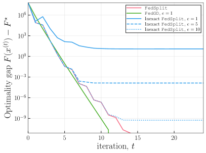
(a) Isotropic case	(b) Spiked case

Figure 2: Plots of the optimality gap $F(x^{(t)})-F^{\star}$ versus the iteration number $t$ for various algorithms as applied to a simple least-squares problem (10). Here $F^{\star}$ denotes the optimal cost value and $F(x^{(t)})$ denote the cost returned at round $t$ by a given algorithm. Shown are curves for inexact and exact implementations of the FedSplit   method and the federated gradient method with $e=1$. The inexact implementations of the FedSplit   method use a gradient method for the approximate proximal updates, and we show curves for number of gradient steps $e\in\{1,5,10\}$. These curves exhibit floors corresponding to the errors introduced by the approximate proximal solves. (a) Isotropic case: results for random design matrices with i.i.d. $\mathsf{N}\left(0,I_{d}\right)$ rows, corresponding to a well-conditioned setting. (b) Spiked case: results for design matrices generated according to the procedure described in Section 4.3 with $\kappa=10$. These problems are somewhat poorly conditioned, causing a slowdown in convergence that is more severe for federated gradient.

We solve the resulting optimization problem using various methods: the FedGD procedure with $e=1$, which is the only setting guaranteed to preserve the fixed points; the exact form of FedSplit procedure, in which the proximal updates are computed exactly; and inexact versions of the FedSplit procedure using the gradient method (see Corollary 1) to compute approximations to the updates with $e\in\{1,5,10\}$ rounds of gradient updates per machine.

Figure 2 shows the results of these experiments, plotting the log optimality gap $\log(F(x^{(t)})-F^{*})$ versus the iteration number $t$ for these algorithms; see the caption for discussion of the behavior.

4.2 Logistic regression

Moving beyond the setting of least squares regression, we now explore the behavior of various algorithms for solving federated binary classification. In this problem, we again have fixed design matrices $A_{j}\in\mathbf{R}^{n_{j}\times d}$, but the response vectors take the form of labels, $b_{j}\in\{1,-1\}^{n_{j}}$. Here the rows of $A_{j}$, denoted by $a_{ij}\in\mathbf{R}^{d}$ for $i=1,\dots,n_{j}$ are collections of $d$ features, associated with class label $b_{ij}\in\{-1,1\}$, the entries of $b_{j}$. We assume that for $j=1,\dots,m$ and unknown parameter vector $x_{0}\in{}^{d}$, the conditional probability of observing a positive class label $b_{ij}=1$ is given by

$$\operatorname{\bf P}\{b_{ij}=1\}=\frac{\mathrm{e}^{a_{ij}^{\mathsf{T}}x_{0}}}{1+\mathrm{e}^{a_{ij}^{\mathsf{T}}x_{0}}},\quad\text{for }i~{}=1,\dots,n_{j}.$$ (26)

Given observations of this form, the maximum likelihood estimate for $x_{0}$ is then a solution to the convex program

$$\text{minimize}\quad\sum_{j=1}^{m}\sum_{i=1}^{n_{j}}\log(1+\mathrm{e}^{-b_{ij}a_{ij}^{\mathsf{T}}x}),$$ (27)

with variable $x\in\mathbf{R}^{d}$. This problem is referred to as logistic regression.

Since the function $t\mapsto\log(1+\mathrm{e}^{-t})$ has bounded, positive second derivative, it is straightforward to verify that the objective function in problem (27) is smooth and convex. The local cost functions $f_{j}\colon\mathbf{R}^{d}\to\mathbf{R}$ are given by the corresponding sums over the local datasets—that is

$$f_{j}(x)\mathrel{\hbox to0.0pt{\raisebox{1.29167pt}{$\cdot$}\hss}\raisebox{-1.29167pt}{$\cdot$}}=\sum_{i=1}^{n_{j}}\log(1+\mathrm{e}^{-b_{ij}a_{ij}^{\mathsf{T}}x}),\qquad\text{for}~{}j=1,\dots,m.$$

With this definition, we see that (27) is equivalent to the minimization of $F(x)=\sum_{j=1}^{m}f_{j}(x)$, which places this problem in the broader framework of federated problems of the form (1).

For the simple experiments reported here, we construct some random instances of logistic regression problems with the settings

$$d=100,\quad n_{j}\equiv 1000,\quad\text{and}\quad m=10,$$

so that the total sample size is $n=10000$. We construct a random instance by drawing the feature vectors $a_{ij}\overset{\text{i.i.d.}}{\sim}\mathsf{N}\left(0,I_{d}\right)$ for $j=1,\dots,m$ and $i=1,\dots,n_{j}$, generating the true parameter randomly as $x_{0}\overset{\text{i.i.d.}}{\sim}\mathsf{N}\left(0,I_{d}\right)$, and then generating the binary labels $b_{ij}$ according to the Bernoulli model (26).

Given this synthetic dataset, we then solve the problem (27) by applying exact implementations of FedSplit   as well as a number of inexact implementations, where each local update is a constant number of gradient steps, $e\in\{1,5,10\}$. For comparison, we also implement a federated gradient method as previously described (8).

Figure 3: Plots of the optimality gap $F(x^{(t)})-F^{\star}$ versus the iteration number $t$ for various algorithms as applied to a logistic regression problem (27). Here $F^{\star}$ denotes the optimal cost value and $F(x^{(t)})$ denote the cost returned at round $t$ by a given algorithm. Shown are curves for inexact and exact implementations of the FedSplit method and the federated gradient method with $e=1$. The inexact implementations of the FedSplit method use a gradient method for the approximate proximal updates, and we show curves for number of gradient steps $e\in\{1,5,10\}$. These curves for $e\in\{1,5\}$ exhibit an error floor (corresponding to the inaccuracy introduced by approximate proximal solves), whereas the curve for $e=10$ tracks the exact procedure to accuracy below $10^{-6}$.

As shown in Figure 3, the results are qualitatively similar to those shown for the least-squares problem. Both FedGD with $e=1$ and the FedSplit procedure exhibit linear convergence rates. Using inexact proximal updates with the FedSplit procedure preserves the linear convergence up to the error floor introduced by the exactness of the updates. In this case, the inexact proximal updates with $e=10$—that is, performing $10$ local updates per each round of global communication—suffice to track the exact FedSplit procedure up to an accuracy below $10^{-6}$.

4.3 Dependence on problem conditioning

It is well-known that the convergence rates of various optimization algorithms can be strongly affected by the conditioning of the problem, and theory makes specific predictions about this dependence, both for the correct form of the FedGD algorithm (implemented with $e=1$), and the FedSplit procedure. In practice, for the machine learning prediction problems, ill-conditioning can arise due to heterogeneous scalings and/or dependencies between different features that are used. Accordingly, it is interesting to study the dependence of procedures on the condition number.

First, let us re-state the theoretical guarantees that are enjoyed by the different procedures. For a given algorithm, its iteration complexity is a measure of the number of iterations, as a function of some error tolerance $\varepsilon>0$ and possibly other problem parameters, required to return a solution that is $\varepsilon$-optimal. More precisely, for a given algorithm, we let $T(\varepsilon,\kappa)$ denote the maximum number of iterations required so that, for any problem with condition number at most $\kappa$, the iterate $x^{T}$ with $T=T(\varepsilon,\kappa)$ satisfies the bound $F(x^{(T)})-F^{\star}\leqslant\varepsilon$. Note that in the federated setting, $T(\varepsilon,\kappa)$ provides an upper bound on the number of communication rounds required to ensure an $\varepsilon$-cost-suboptimal point to the federated optimization problem that is being solved. Since communication is very often the dominant cost in carrying out such numerical procedures, it is of great interest to make $T(\varepsilon,\kappa)$ as small as possible.

As mentioned in Section 2.1, classical results guarantee that the federated gradient procedure (8), when implemented with the number of gradient steps $e=1$, enjoys linear convergence. More precisely, given the federated objective $F(z)=\sum_{j=1}^{m}f_{j}(z_{j})$, we define its condition number as $\kappa=L^{\ast}/\ell_{\ast}$. Then FedGD has an iteration complexity bounded as

$$T_{\rm FedGrad}(\varepsilon,\kappa)=O(\kappa\log(1/\varepsilon)).$$ (28a)

On the other hand, it follows from Theorem 1 that the FedSplit procedure has iteration complexity scaling as

$$T_{\rm FedSplit}(\varepsilon,\kappa)=O(\sqrt{\kappa}\log(1/\varepsilon)).$$ (28b)

Thus, albeit at the expense of a more expensive local update, the FedSplit   procedure has better dependence on the condition number than federated gradient descent. This highlights an important tradeoff between local computation and global communication in these methods.

We now describe the results of a simulation study that demonstrates the accuracy of these predicted iteration complexities. At a high level, our strategy is to construct a sequence of problems, indexed by an increasing sequence of condition numbers $\kappa$, and to estimate the number of iterations required to achieve a given tolerance $\varepsilon>0$ as a function of $\kappa$. In order to do, it suffices to consider ensembles of least squares problems (10), but with a carefully constructed collection of design matrices, which we now describe.

For a given integer $\ell\geqslant 2$, let $\mathrm{O}(\ell)$ denote the set of $\ell\times\ell$ orthogonal matrices over the reals, and let $\mathsf{Unif}(\mathrm{O}(\ell))$ denote the uniform (Haar) measure on this compact group. With this notation, we begin by sampling i.i.d.random matrices

$$U_{j}^{(\kappa)}\sim\mathsf{Unif}(\mathrm{O}(n_{j}))\quad\text{and}\quad V_{j}^{(\kappa)}\sim\mathsf{Unif}(\mathrm{O}(d)),\qquad\text{for $j=1,\ldots,m$.}$$ (29)

For a given condition number $\kappa\geqslant 1$, we define a padded diagonal matrix—that is

$$\Lambda_{j}^{(\kappa)}=\begin{bmatrix}\operatorname{\bf diag}(\lambda_{j}^{(\kappa)})&0_{d,(n-d)}\end{bmatrix}\quad\text{where}\quad\lambda_{j}^{(\kappa)}=(\sqrt{\kappa},1,\dots,1)\in\mathbf{R}^{d}.$$

Above, the matrix $0_{d,(n_{j}-d)}\in\mathbf{R}^{d\times(n_{j}-d)}$ has all entries equal to zero. Given the random orthogonal matrices and the matrix $\Lambda_{j}^{(\kappa)}\in\mathbf{R}^{n_{j}\times d}$, we then construct the design matrices $A_{j}^{(\kappa)}\in\mathbf{R}^{n_{j}\times d}$ by setting

$$A_{j}^{(\kappa)}\mathrel{\hbox to0.0pt{\raisebox{1.29167pt}{$\cdot$}\hss}\raisebox{-1.29167pt}{$\cdot$}}=U_{j}^{(\kappa)}\Lambda_{j}^{(\kappa)}V_{j}^{(\kappa)},\quad\text{for all }~{}j=1,\dots,m.$$

These choices ensure that the federated least squares objective (10) has condition number $\kappa$.

As before, the response vectors $b_{j}^{(\kappa)}$ obey a Gaussian linear measurement model,

$$b_{j}^{(\kappa)}=A_{j}^{(\kappa)}x_{0}+v_{j}^{(\kappa)},\quad\text{for}~{}j=1,\dots,m,\quad\text{and for all}~{}\kappa\in K.$$

We again take $v_{j}^{(\kappa)}\overset{\textrm{ind.}}{\sim}\mathsf{N}\left(0,\sigma^{2}I_{n_{j}}\right)$. In our experiments, we draw the parameter $x_{0}\sim\mathsf{N}\left(0,I_{d}\right)$, and use the parameter settings

$$m=10,\quad d=100,\quad n_{j}\equiv 400,\quad\mbox{and}\quad\sigma^{2}=1.$$

With these settings, we iterated over a collection of condition numbers $\kappa\in\{10^{0},10^{0.5},\dots,10^{3.5},10^{4}\}$. For each choice of $\kappa$, after generating a random instance as described above, we measured the number of iterations required for FedGD and the FedSplit procedures, respectively, to reach a target accuracy $\varepsilon=10^{-3}$, which is modest at best.

(a)

(b)

Figure 4: Dependence of algorithms on the conditioning. (a) Plot of log cost suboptimality of iterate $x^{(t)}$ versus iteration $t$ for condition number $\kappa\in\{100,1000,10000\}$. Consistent with theory, both procedures exhibit geometric convergence, with the rates decaying as the condition number $\kappa$ increases. Note that the FedGD procedure degrades more rapidly than the FedSplit procedure as $\kappa$ is increased. (b) Plots of the iteration complexity $T(\varepsilon;\kappa)$ versus $\kappa$ at tolerance level $\varepsilon=10^{-3}$ for the FedGD and FedSplit procedures. It measures the number of iterations required to achieve an $\varepsilon=10^{-3}$ accurate solution for a problem with condition number $\kappa$. Consistent with their theoretical guarantees, FedGD exhibits linear dependence, whereas the FedSplit procedure exhibits sublinear dependence.

In this way, we obtain estimates of the functions $\kappa\mapsto T_{\rm FedGrad}(10^{-3},\kappa)$ and $\kappa\mapsto T_{\rm FedSplit}(10^{-3},\kappa)$, which measure the dependence of the iteration complexity on the condition number. Figure 4 provides plots of these estimated functions. Consistent with the theory, we see that FedGD has an approximately linear dependence on the condition number, whereas the FedSplit procedure has much milder dependence on conditioning. Concretely, for an instance with condition number $\kappa=10000$, the FedGD procedure requires on the order of $34000$ iterations, whereas the FedSplit procedure requires roughly $400$ iterations. Again, to be fair, the FedSplit involves more complicated proximal updates at each client, so that these iteration counts should be viewed as reflecting the number of rounds of communication between the individual clients and the centralized server, as opposed to total computational complexity.

5 Proofs

We now turn to the proofs of our main results. Prior to diving into these arguments, we first introduce two operators that play a critical role in our analysis. Given a convex function $\varphi\colon\mathbf{R}^{d}\to\mathbf{R}$, we define

$$\operatorname{\bf prox}_{\varphi}(z) \mathrel{\hbox to0.0pt{\raisebox{1.29167pt}{$\cdot$}\hss}\raisebox{-1.29167pt}{$\cdot$}}=\mathop{\rm arg\,min}_{x\in\mathbf{R}^{d}}\left\{\varphi(x)+\frac{1}{2}\|z-x\|^{2}\right\}\quad\text{and}\quad$$ (30a)

$$\operatorname{\bf refl}_{\varphi}(z) \mathrel{\hbox to0.0pt{\raisebox{1.29167pt}{$\cdot$}\hss}\raisebox{-1.29167pt}{$\cdot$}}=2\operatorname{\bf prox}_{\varphi}(z)-z.$$ (30b)

These are called the proximal and reflected resolvent operators associated with the function $\varphi$. The first operator is also known as the resolvent; the second operator above is also known as the Cayley operator of $\varphi$. Moreover, our analysis makes use of the (semi)norm on Lipschitz continuous functions $f\colon\mathbf{R}^{d}\to\mathbf{R}$ given by

$$\operatorname{Lip}(f)\mathrel{\hbox to0.0pt{\raisebox{1.29167pt}{$\cdot$}\hss}\raisebox{-1.29167pt}{$\cdot$}}=\sup_{x\neq y}\frac{|f(x)-f(y)|}{\|x-y\|}.$$ (31)

For short, we say that that $f$ is $\operatorname{Lip}(f)$-Lipschitz continuous when it satisfies this condition.

5.1 Proofs of guarantees for FedSplit

We begin by proving our guarantees for the FedSplit procedure, including the correctness of its fixed points (Proposition 3); the general convergence guarantee in the strongly convex case (Theorem 1); the general convergence guarantee in the weakly convex case (Theorem 2), and Corollary 1 on its convergence with approximate proximal updates.

5.2 Proof of Proposition 3

By the fixed point assumption, the block average $x^{\star}\mathrel{\hbox to0.0pt{\raisebox{1.29167pt}{$\cdot$}\hss}\raisebox{-1.29167pt}{$\cdot$}}=\overline{z^{\star}}$ satisfies the relation

$$\operatorname{\bf prox}_{sf_{j}}(2x^{\star}-z^{\star}_{j})=x^{\star}\qquad\mbox{for $j=1,2,\ldots,m$.}$$

Since each $f_{j}$ is convex and differentiable, by the first-order stationary conditions implied by the definition of the prox operator (30a), we must have

$$\nabla f_{j}(x^{\star})+\tfrac{1}{s}\big{\{}x^{\star}-\big{(}2x^{\star}-z^{\star}_{j})\big{\}}\;=\;\nabla f_{j}(x^{\star})+\tfrac{1}{s}\big{\{}z^{\star}_{j}-x^{\star}\big{\}}\;=\;0\quad\mbox{for $j=1,\ldots,m$.}$$

Summing these equality relations over $j=1,\ldots,m$ and using the fact that $x^{\star}=\tfrac{1}{m}\sum_{j=1}^{m}z^{\star}_{j}$ yields the zero gradient condition

$$\sum_{j=1}^{m}\nabla f_{j}(x^{\star})\;=\;0.$$

Since the function $x\mapsto\sum_{j=1}^{m}f_{j}(x)$ is convex, this zero-gradient condition implies that $x^{\star}\in{}^{d}$ is a minimizer of the distributed problem as claimed.

5.2.1 Proof of Theorem 1

We now turn to the proof of Theorem 1. Our strategy is to prove it as a consequence of a somewhat more general result, which we begin by stating here. In order to lighten notation, we use the fact that the proximal operator for the function $F(z_{1},\ldots,z_{m})=\sum_{j=1}^{m}f_{j}(z_{j})$ is block-separable, so that in terms of the block-partitioned vector $z=(z_{1},\ldots,z_{m})$, we can write

$$\operatorname{\bf prox}_{sF}(z)=\left(\operatorname{\bf prox}_{sf_{1}}(z_{1}),\dots,\operatorname{\bf prox}_{sf_{m}}(z_{m})\right),\quad\mbox{for all $z=(z_{1},\dots,z_{m})\in({}^{d})^{m}$.}$$

We also recall the the approximate proximal operator used in the FedSplit procedure, namely

$$\widetilde{\operatorname{\bf prox}}(z)\mathrel{\hbox to0.0pt{\raisebox{1.29167pt}{$\cdot$}\hss}\raisebox{-1.29167pt}{$\cdot$}}=\left(\mathtt{prox\_update}_{1}(z_{1}),\dots,\mathtt{prox\_update}_{m}(z_{m})\right),\quad\text{for all}~{}z_{1},\dots,z_{m}\in\mathbf{R}^{d}.$$

Theorem 3 (Convergence with general residuals).

Suppose that the functions $f_{j}\colon\mathbf{R}^{d}\to\mathbf{R}$ are $\ell_{j}$-strongly convex and $L_{j}$-smooth for $j=1,\ldots,m$, and for $t=1,2,\ldots$, define the residuals

$$r^{(t)}\mathrel{\hbox to0.0pt{\raisebox{1.29167pt}{$\cdot$}\hss}\raisebox{-1.29167pt}{$\cdot$}}=\widetilde{\operatorname{\bf prox}}(2\overline{z^{(t)}}-z^{(t)})-\operatorname{\bf prox}_{sF}(2\overline{z^{(t)}}-z^{(t)}).$$ (32)

Then with stepsize $s=1/\sqrt{\ell_{\ast}L^{\ast}}$, the FedSplit procedure (Algorithm 3.2) has a unique fixed point $z^{\star}$, and the iterates satisfy

$$\|z^{(t+1)}-z^{\star}\| \leqslant\rho^{t}\|z^{(1)}-z^{\star}\|+2\sum_{j=1}^{t}\rho^{t-j}\|r^{(j)}\|\qquad\mbox{for $t=1,2,\ldots$,}$$ (33)

where $\rho\mathrel{\hbox to0.0pt{\raisebox{1.29167pt}{$\cdot$}\hss}\raisebox{-1.29167pt}{$\cdot$}}=1-2/(\sqrt{\kappa}+1)$ is the contraction coefficient.

Let us use Theorem 3 to derive the claim stated in Theorem 1. Note that by Proposition 3, the fixed points of Algorithm 3.2 are minimizers of $F$, hence unique under the strong convexity assumption. Consequently, we have

$$\|x^{(t+1)}-x^{\star}\|\leqslant\frac{1}{\sqrt{m}}\|z^{(t+1)}-z^{\star}\|,\qquad\mbox{for all $t=1,2,\ldots$.}$$

Using Theorem 3 and the error bound, we then conclude that

$$\|x^{(t+1)}-x^{\star}\|\leqslant\frac{1}{\sqrt{m}}\left(1-\frac{2}{\sqrt{\kappa}+1}\right)^{\!t}\|z^{(1)}-z^{\star}\|+(\sqrt{\kappa}+1)b,$$

as claimed.

5.2.2 Proof of Theorem 3

We now turn to the proof of the more general claim. Given additive decomposition $F(z)=\sum_{j=1}^{m}f_{j}(z_{j})$, the reflected resolvent induced by $F$ is block-separable, taking the form

$$\operatorname{\bf refl}_{sF}(z)=\left(\operatorname{\bf refl}_{sf_{1}}(z_{1}),\dots,\operatorname{\bf refl}_{sf_{m}}(z_{m})\right),\quad\mbox{for all $z=(z_{1},\dots,z_{m})\in(\mathbf{R}^{d})^{m}$.}$$

Similarly, consider the approximate reflected resolvent defined by the algorithm, namely

$$\widetilde{\operatorname{\bf refl}}(z)\mathrel{\hbox to0.0pt{\raisebox{1.29167pt}{$\cdot$}\hss}\raisebox{-1.29167pt}{$\cdot$}}=2\widetilde{\operatorname{\bf prox}}(z)-z,\quad\mbox{for all $z=(z_{1},\ldots,z_{m})\in(\mathbf{R}^{d})^{m}$.}$$

It also has the same block-separable form.

Using these two block-separable operators, we can now define two abstract operators, each acting on the product space $({}^{d})^{m}$, that allow us to analyze the algorithm. The first operator $\mathcal{T}$ underlies the idealized algorithm, in which the proximal updates are exact, and the second operator $\widehat{\mathcal{T}}$ underlies the practical algorithm, which is based on approximate proximal updates. The idealized algorithm is based on iterating the operator

$$\mathcal{T}(z)\mathrel{\hbox to0.0pt{\raisebox{1.29167pt}{$\cdot$}\hss}\raisebox{-1.29167pt}{$\cdot$}}=\operatorname{\bf refl}_{sF}\big{(}\operatorname{\bf refl}_{I_{E}}(z)\big{)}.$$ (34)

In this definition, we use $I_{E}$ to denote the indicator function for membership in the equality subspace $E$, so that $\operatorname{\bf refl}_{I_{E}}$ is the reflected proximal operator for this function.

On the other hand, the practical algorithm generates the sequence $\{z^{(t)}\}_{t=1}^{\infty}$ via the updates $z^{(t+1)}=\widehat{\mathcal{T}}(z^{(t)})$, where $\widehat{\mathcal{T}}:({}^{d})^{m}\rightarrow({}^{d})^{m}$ is the perturbed operator

$$\widehat{\mathcal{T}}(z) =\widetilde{\operatorname{\bf refl}}\big{(}\operatorname{\bf refl}_{I_{E}}(z)\big{)}.$$ (35)

Note that the idealized operator $\mathcal{T}$ and perturbed operator $\widehat{\mathcal{T}}$ satisfy the relation

$$\widehat{\mathcal{T}}-\mathcal{T} =\left(\widetilde{\operatorname{\bf refl}}\circ\operatorname{\bf refl}_{I_{E}}-\operatorname{\bf refl}_{sF}\circ\operatorname{\bf refl}_{I_{E}}\right).$$ (36)

Our proof involves verifying that with the stepsize choice $s=1/\sqrt{\ell_{\ast}L^{\ast}}$, the mapping $\mathcal{T}$ is a contraction, with Lipschitz coefficient

$$\operatorname{Lip}(\mathcal{T}) \leqslant\underbrace{1-\frac{2}{\sqrt{\kappa}+1}}_{\mbox{$=\mathrel{\hbox to0.0pt{\raisebox{0.90417pt}{$\cdot$}\hss}\raisebox{-0.90417pt}{$\cdot$}}\rho$}}<1.$$ (37)

Taking this claim as given for the moment, the contractivity implies that $\mathcal{T}$ has has a unique fixed point [12]—call it $z^{\star}\in({}^{d})^{m}$. Comparing with Proposition 3, we see that the definition of fixed points given there agrees with the fixed point $z^{\star}$ of the operator $\mathcal{T}$, since we have the relation $\operatorname{\bf refl}_{I_{E}}(z)=2\overline{z}-z$.

Using this contractivity condition, the distance between this fixed point $z^{\star}$ and the iterates $z^{(t)}$ of the FedSplit procedure can be bounded as

$$\|z^{(t+1)}-z^{\star}\| =\|\widehat{\mathcal{T}}z^{(t)}-\mathcal{T}z^{\star}\|$$

$$\stackrel{{\scriptstyle\rm(i)}}{{\leqslant}}\|\mathcal{T}z^{(t)}-\mathcal{T}z^{\star}\|+2\|\widetilde{\operatorname{\bf prox}}\operatorname{\bf refl}_{I_{E}}z^{(t)}-\operatorname{\bf prox}_{sF}\operatorname{\bf refl}_{I_{E}}z^{(t)}\|$$

$$\stackrel{{\scriptstyle\rm(ii)}}{{\leqslant}}\operatorname{Lip}(\mathcal{T})\|z^{(t)}-z^{\star}\|+2\|r^{(t)}\|$$

$$\stackrel{{\scriptstyle\rm(iii)}}{{\leqslant}}\rho\|z^{(t)}-z^{\star}\|+2\|r^{(t)}\|,$$ (38)

where inequality (i) applies the triangle inequality to the relation (36) between the perturbed and idealized operators; step (ii) follows by definition of the residual $r^{(t)}$ at round $t$; and step (iii) follows from the bound (37) on the Lipschitz coefficient of $\mathcal{T}$. Performing induction on this bound yields the stated claim.

Proof of the bound (37):

It remains to bound the Lipschitz coefficient of the idealized operator $\mathcal{T}$. Since the composite function $F(z)\mathrel{\hbox to0.0pt{\raisebox{1.29167pt}{$\cdot$}\hss}\raisebox{-1.29167pt}{$\cdot$}}=\sum_{j=1}^{m}f_{j}(z_{j})$ is $\ell_{\ast}$-strongly convex and $L^{\ast}$-smooth, known results on reflected proximal operators [11, Theorems 1 and 2] imply that with the stepsize choice $s=1/\sqrt{\ell_{\ast}L^{\ast}}$, the operator $\operatorname{\bf refl}_{sF}$ satisfies the bound

$$\|\operatorname{\bf refl}_{sF}(z)-\operatorname{\bf refl}_{sF}(z^{\prime})\|_{2} \leqslant\Big{(}1-\frac{2}{\sqrt{\kappa}+1}\Big{)}\|z-z^{\prime}\|_{2}\qquad\mbox{for all $z,z^{\prime}\in({}^{d})^{m}$.}$$ (39)

On the other hand, the reflected proximal operator $\operatorname{\bf refl}_{I_{E}}$ for the indicator function $\operatorname{\bf refl}_{I_{E}}$ is non-expansive, so that

$$\|\operatorname{\bf refl}_{I_{E}}(z)-\operatorname{\bf refl}_{I_{E}}(z)\|_{2} \leqslant\|z-z^{\prime}\|_{2}\qquad\mbox{for all $z,z^{\prime}\in({}^{d})^{m}$.}$$ (40)

Applying the triangle inequality and using the definition (34) of the idealized operator $\mathcal{T}$, we find that

$$\|\mathcal{T}(z)-\mathcal{T}(z^{\prime})\|_{2} \leqslant\|\operatorname{\bf refl}_{sF}\big{(}\operatorname{\bf refl}_{I_{E}}(z)\big{)}-\operatorname{\bf refl}_{sF}\big{(}\operatorname{\bf refl}_{I_{E}}(z^{\prime})\big{)}\|_{2}$$

$$\stackrel{{\scriptstyle\rm(iv)}}{{\leqslant}}\Big{(}1-\frac{2}{\sqrt{\kappa}+1}\Big{)}\;\|\operatorname{\bf refl}_{I_{E}}(z)-\operatorname{\bf refl}_{I_{E}}(z^{\prime})\|_{2}$$

$$\stackrel{{\scriptstyle\rm(v)}}{{\leqslant}}\Big{(}1-\frac{2}{\sqrt{\kappa}+1}\Big{)}\;\|z-z^{\prime}\|_{2},$$

where step (iv) uses the contractivity (39) of the operator $\operatorname{\bf refl}_{sF}$, and step (v) uses the non-expansiveness (40) of the operator $\operatorname{\bf refl}_{I_{E}}$. This completes the proof of the bound (37).

5.2.3 Proof of Corollary 1

By construction, the function $h_{j}$ is smooth with parameter $M\mathrel{\hbox to0.0pt{\raisebox{1.29167pt}{$\cdot$}\hss}\raisebox{-1.29167pt}{$\cdot$}}=sL^{\ast}+1$ and strongly convex with parameter $m\mathrel{\hbox to0.0pt{\raisebox{1.29167pt}{$\cdot$}\hss}\raisebox{-1.29167pt}{$\cdot$}}=s\ell_{\ast}+1$. Consequently, if we define the operator $H_{j}(u)\mathrel{\hbox to0.0pt{\raisebox{1.29167pt}{$\cdot$}\hss}\raisebox{-1.29167pt}{$\cdot$}}=u-\alpha\nabla h_{j}(u)$, then by standard results on gradient methods for smooth-convex functions, the stepsize choice $\alpha=\frac{2}{M+m}$ ensures that the operator $H_{j}$ is contractive with parameter at least $\rho=1-\frac{m}{M}$. Thus, we have the bound

$$\|u^{(e+1)}-u^{*}\|_{2} \leqslant\rho^{e}\|u^{(1)}-u^{*}\|_{2},$$

where $u^{*}=\operatorname{\bf prox}_{sf_{j}}(x_{j}^{(t)})$ is the optimum of the proximal subproblem. Unpacking the definitions of $(m,M)$ and recalling that $s=1/\sqrt{\ell_{\ast}L^{\ast}}$, we have

$$\frac{M}{m}=\frac{sL^{\ast}+1}{s\ell_{\ast}+1}\;=\;\frac{\sqrt{\frac{L^{\ast}}{\ell_{\ast}}}+1}{\sqrt{\frac{\ell_{\ast}}{L^{\ast}}}+1}\leqslant\;\sqrt{\kappa}+1,$$

and hence $\rho\leqslant 1-\frac{1}{\sqrt{\kappa}+1}$, which establishes the claim.

5.2.4 Proof of Theorem 2

Recalling the definition (24) of the regularized objective $F_{\lambda}$, note that it is related to the unregularized objective $F$ via the relation $F_{\lambda}(x)=F(x)+\frac{m\lambda}{2}\|x-x^{(1)}\|^{2}$, where $x^{(1)}$ is the given initialization. The proposed procedure is to compute an approximation to the quantity

$$x^{\star}_{\lambda}\mathrel{\hbox to0.0pt{\raisebox{1.29167pt}{$\cdot$}\hss}\raisebox{-1.29167pt}{$\cdot$}}=\mathop{\rm arg\,min}_{x\in\mathbf{R}^{d}}\Bigg{(}\underbrace{\sum_{j=1}^{m}\Big{\{}f_{j}(x)+\frac{\lambda}{2}\|x-x^{(1)}\|^{2}\Big{\}}}_{=:F_{\lambda}(x)}\Bigg{)}.$$

Now suppose that we have computed a vector $\widehat{x}\in{}^{d}$ satisfies $F_{\lambda}(\widehat{x})-F_{\lambda}(x^{\star}_{\lambda})\leqslant\varepsilon/2$. Letting $F^{\star}=F(x^{\star})$ denote the optimal value of the original (unregularized) optimization problem, we have

$$F(\widehat{x})-F^{\star} =\Big{\{}F(\widehat{x})-F_{\lambda}(x^{\star}_{\lambda})\Big{\}}+\Big{\{}F_{\lambda}(x^{\star}_{\lambda})-F(x^{\star})\Big{\}}.$$ (41)

By definition of $F_{\lambda}$, we have $F(\widehat{x})\leqslant F_{\lambda}(\widehat{x})$. Moreover, again using the definition of $F_{\lambda}$, we have

$$F_{\lambda}(x^{\star}_{\lambda})-F(x^{\star}) =F_{\lambda}(x^{\star}_{\lambda})-F_{\lambda}(x^{\star})+\frac{m\lambda}{2}\|x^{\star}-x^{(1)}\|^{2}$$

$$\leqslant\frac{m\lambda}{2}\|x^{\star}-x^{(1)}\|^{2},$$

where the inequality follows since $x^{\star}_{\lambda}$ minimizes $F_{\lambda}$ by definition. Substituting these bounds into the initial decomposition (41), we find that

$$F(\widehat{x})-F^{\star} \leqslant\Big{\{}F_{\lambda}(\widehat{x})-F_{\lambda}(x^{\star}_{\lambda})\Big{\}}+\frac{m\lambda}{2}\|x^{\star}-x^{(1)}\|^{2}$$

$$\leqslant\frac{\varepsilon}{2}+\frac{\varepsilon}{2}=\varepsilon.$$ (42)

where the inequality follows since since $\widehat{x}$ is $(\varepsilon/2)$-cost-suboptimal for $F_{\lambda}$, and by our selection of $\lambda$. Thus to finish the proof, we simply need to check how many iterations it takes to compute an $(\varepsilon/2)$-cost-suboptimal point for $F_{\lambda}$.

Let us define the shorthand notation $\overline{L}\mathrel{\hbox to0.0pt{\raisebox{1.29167pt}{$\cdot$}\hss}\raisebox{-1.29167pt}{$\cdot$}}=\sum_{j=1}^{m}L_{j}$ and $\kappa_{\lambda}\mathrel{\hbox to0.0pt{\raisebox{1.29167pt}{$\cdot$}\hss}\raisebox{-1.29167pt}{$\cdot$}}=\frac{L^{\ast}+\lambda}{\lambda}$ Since $F_{\lambda}$ is a sum of functions that are $\lambda$-strongly convex and $(L_{j}+\lambda)$-smooth, it follows that from initialization $x^{(1)}$, the FedSplit algorithm outputs iterates $x^{(t)}$ satisfying the bound

$$F_{\lambda}(x^{(t+1)})-F_{\lambda}(x^{\star}_{\lambda}) \stackrel{{\scriptstyle\rm(i)}}{{\leqslant}}\frac{\overline{L}+m\lambda}{2}\|x^{(t+1)}-x^{\star}_{\lambda}\|^{2}$$

$$\stackrel{{\scriptstyle\rm(ii)}}{{\leqslant}}\frac{\overline{L}+m\lambda}{2}\left(1-\frac{2}{\sqrt{\kappa_{\lambda}}+1}\right)^{\!2t}\frac{\|x^{(1)}-z^{\star}_{\lambda}\|^{2}}{m}.$$ (43)

In the above reasoning, inequality (i) is a consequence of the smoothness of the losses $f_{j}$ when regularized by $\lambda$, along with the first-order optimality condition for $x^{\star}_{\lambda}$; and bound (ii) then follows by squaring the guarantee of Theorem 1 with $b=0$. By inverting the bound (43), we see that in order to achieve an $\varepsilon/2$-optimal solution, it suffices to take the number of iterations $t$ to be lower bounded as

$$t\geqslant\left\lceil\frac{\sqrt{\kappa_{\lambda}}+1}{4}\log\left\{\frac{(\overline{L}+\lambda m)\|x^{(1)}-z^{\star}_{\lambda}\|^{2}}{m}\right\}\right\rceil.$$

Evaluating this bound with the choice $\kappa_{\lambda}=1+L^{\ast}/\lambda$ and recalling the bound (42) yields the claim of the theorem.

5.3 Characterization of fixed points

In this section we give the two fixed point results for FedSGD and FedProx as stated in Section 3.1.

5.3.1 Proof of Proposition 1

We begin by characterizing the fixed points of the FedSGD algorithm. By definition, any limit point $(x_{1}^{\star},\dots,x_{m}^{\star})\in({}^{d})^{m}$ must satisfy the fixed point relation

$$x^{\star}_{j}=\frac{1}{m}\sum_{j=1}^{m}G_{j}^{e}(x^{\star}_{j}),\qquad j=1,2,\ldots,m.$$

Thus, the limits $x_{j}^{\star}$ are common, and this gives part (a) of the claim. Expanding the iterated operator $G_{j}^{e}$ gives part (b).

5.3.2 Proof of Proposition 2

We now characterize the fixed points of the FedProx algorithm. By definition, any limit point $(x_{1}^{\star},\dots,x_{m}^{\star})$ satisfies

$$x^{\star}_{j}=\frac{1}{m}\sum_{j=1}^{m}\operatorname{\bf prox}_{sf_{j}}(x^{\star}_{j}),\qquad j=1,2,\ldots,m.$$ (44)

Thus, the limits $x_{j}^{\star}$ are common, and this gives part (a) of the claim.

For any convex function, $f\colon\mathbf{R}^{d}\to\mathbf{R}$, the proximal operator satisfies

$$\operatorname{\bf prox}_{sf}(v)=v-s\nabla M_{sf}(v),\quad\text{for all}~{}s>0~{}\text{and}~{}v\in\mathbf{R}^{d}.$$

Using this identity in display (44) yields part (b) of the claim.

6 Discussion

In this paper, we have studied the problem of federated optimization, in which the goal is to minimize a sum of functions, with each function assigned to a client, using a combination of local updates at the client and a limited number of communication rounds. We began by showing that some previously proposed methods for federated optimization, even when considered in the simpler setting of convex and deterministic updates, need not have fixed points that correspond to the optima of original problem. We addressed this issue by proposing and analyzing a new scheme known as FedSplit, based on operator splitting. We showed that it that does indeed retain the correct fixed points and we provided convergence guarantees for various forms of convex minimization problems (Theorems 1 and 2).

This paper leaves open a number of questions. First of all, the analysis of this paper was limited to deterministic algorithms, whereas in practice, one typically uses stochastic approximations to gradient updates. In the context of the FedSplit procedure, it is natural to consider stochastic approximations to the proximal updates that underlie it. Given our results on the incorrectness of previously proposed methods and the work of Woodworth and colleagues [30] on the suboptimality on multi-step stochastic gradient methods, it is interesting to develop a precise characterization of the tradeoff between the accuracy of stochastic and deterministic approximations to intermediate quantities and rates of convergence in federated optimization. It is also interesting to consider stochastic approximation methods that exploit higher-order information, such as the Newton sketch algorithm and other second-order subsampling procedures [22, 23].

Moreover, the current paper assumed that updates at all clients are performed synchronously, whereas in federated problems, often the client updates are carried out asynchronously. We thus intend to explore how the FedSplit and related splitting procedures behave under stragglers and delays in computation. Finally, an important desideratum in federated learning is that local updates are carried out with suitable privacy guarantees for the local data [3]. Understanding how noise aggregated through differentially private mechanisms couples with our inexact convergence guarantees is a key direction for future work.

Acknowledgements

We thank Bora Nikolic for his careful reading and comments on an initial draft of this manuscript. RP was partially supported by a Berkeley ARCS Fellowship. MJW was partially supported by Office of Naval Research grant DOD-ONR-N00014-18-1-2640, and NSF grant NSF-DMS-1612948.

References

- [1] H. H. Bauschke and P. L. Combettes. Convex analysis and monotone operator theory in Hilbert spaces. Springer, 2nd edition, 2017.
- [2] D. P. Bertsekas and J. N. Tsitsiklis. Parallel and Distributed Computation: Numerical Methods. Athena Scientific, Boston, MA, 1997.
- [3] A. Bhowmick, J. Duchi, J. Freudiger, G. Kapoor, and R. Rogers. Protection against reconstruction and its applications in private federated learning. Technical report, 2018. arxiv.org:1812.00984.
- [4] K. Bonawitz, H. Eichner, et al. Towards federated learning at scale: System design. Technical report, February 2019. arxiv.org:1902.01046.
- [5] S. Boyd, N. Parikh, E. Chu, B. Peleato, and J. Eckstein. Distributed optimization and statistical learning via the alternating direction method of multipliers. Foundations and Trends in Machine Learning, 3(1):1–122, 2010.
- [6] S. Boyd and L. Vandenberghe. Convex optimization. Cambridge University Press, Cambridge, UK, 2004.
- [7] P. L. Combettes. Monotone operator theory in convex optimization. Math. Program., 170(1, Ser. B):177–206, 2018.
- [8] O. Dekel, R. Gilad-Bachrach, O. Shamir, and L. Xiao. Optimal distributed online prediction using mini-batches. J. Mach. Learn. Res., 13(1):165––202, January 2012.
- [9] S. Diamond and S. Boyd. CVXPY: A Python-embedded modeling language for convex optimization. J. Mach. Learn. Res., 17(83):1–5, 2016.
- [10] P. Giselsson. Tight global linear convergence rate bounds for Douglas-Rachford splitting. J. Fixed Point Theory Appl., 19(4):2241—2270, 2017.
- [11] P. Giselsson and S. Boyd. Linear convergence and metric selection for Douglas-Rachford splitting and ADMM. IEEE Trans. Automatic Control, 62(2):532–544, February 2017.
- [12] K. Goebel and W. A. Kirk. Topics in metric fixed point theory, volume 28 of Cambridge Studies in Advanced Mathematics. Cambridge University Press, Cambridge, 1990.
- [13] P. Kairouz, H. B. McMahan, et al. Advances and open problems in federated learning. Technical report, December 2019. arXiv.org:1912.04977.
- [14] S. Lacoste-Julien, M. Schmidt, and F. Bach. A simpler approach to obtaining an convergence rate for the projected stochastic subgradient method. Technical Report arxiv.org/abs/1212.2002, December 2012.
- [15] M. Li, D. G. Andersen, A. J. Smola, and K. Yu. Communication efficient distributed machine learning with the parameter server. In Advances in Neural Information Processing Systems 27, pages 19—27. Curran Associates, Inc., 2014.
- [16] T. Li, A. K. Sahu, A. Talwalkar, and V. Smith. Federated learning: challenges, methods and future directions. Technical Report arxiv.org/abs/1908.07873, August 2019.
- [17] T. Li, A. K. Sahu, M. Zaheer, M. Sanjabi, A. Talwalkar, and V. Smith. Federated optimization in heterogeneous networks. Technical Report arxiv.org/abs/1812.06127, December 2018.
- [18] H. B. McMahan, E. Moore, D. Ramage, S. Hampson, and B. A. Arcas. Communication-efficient learning of deep networks from decentralized data. Technical Report arxiv.org/abs/1602.05629, February 2016.
- [19] W. M. Moursi and L. Vandenberghe. Douglas-Rachford splitting for the sum of a Lipschitz continuous and a strongly monotone operator. J. Optimization Theory and Applications, 183(1):179–198, 2019.
- [20] N. Parikh, S. Boyd, et al. Proximal algorithms. Foundations and Trends® in Optimization, 1(3):127–239, 2014.
- [21] D. W. Peaceman and Jr. H. H. Rachford. The numerical solution of parabolic and elliptic differential equations. Journal of the SIAM, 3(1):28–41, March 1955.
- [22] M. Pilanci and M. J. Wainwright. Iterative Hessian Sketch: Fast and accurate solution approximation for constrained least-squares. Journal of Machine Learning Research, 17(53):1–38, April 2016.
- [23] M. Pilanci and M. J. Wainwright. Newton sketch: A linear-time optimization algorithm with linear-quadratic convergence. SIAM Jour. Opt., 27(1):205–245, March 2017.
- [24] P. Richtárik and M. Takáč. Distributed coordinate descent method for learning with big data. J. Mach. Learn. Res., 17(1):2657—2681, January 2016.
- [25] R. T. Rockafellar. Convex Analysis. Princeton University Press, Princeton, 1970.
- [26] R. T. Rockafellar. Monotone operators and the proximal point algorithm. SIAM J. Control Optim., 14(5):877–898, 1976.
- [27] R.T. Rockafellar and R. J-B Wets. Variational Analysis, volume 317. Springer Science & Business Media, 2009.
- [28] E. K. Ryu and S.P. Boyd. Primer on monotone operator methods. Applied Computational Mathematics: an Interational Journal, 15(1):3–43, 2016.
- [29] M. J. Wainwright. High-dimensional statistics: A non-asymptotic viewpoint. Cambridge University Press, Cambridge, UK, 2019.
- [30] B. E. Woodworth, K. K. Patel, S. U. Stich, Z. Dai, B. Bullins, H. B. McMahan, O. Shamir, and N. Srebro. Is local SGD better than minibatch SGD? Technical report, 2020. arxiv.org:2002.07839.
- [31] Y. Zhang, J. C. Duchi, and M. J. Wainwright. Communication-efficient algorithms for statistical optimization. J. Mach. Learn. Res., 14(68):3321—3363, 2013.