The Dynamics of Quantum Correlations
of Two Qubits in a Common Environment
Modeled by Large Random Matrices

Abstract

This paper is a continuation of our previous paper [8], in which we have studied the dynamics of quantum correlations of two qubits embedded each into its own disordered multiconnected environment. We modeled the environment by random matrices of large size allowing for a possibility to describe meso- and even nanoenvironments. In this paper we also study the dynamics of quantum correlations of two qubits but embedded into a common environment which we also model by random matrices of large size. We obtain the large size limit of the reduced density matrix of two qubits. We then use an analog of the Bogolyubov-van Hove (also known as the Born-Markov) approximation of the theory of open systems and statistical mechanics. The approximation does not imply in general the Markovian evolution in our model but allows for sufficiently detailed analysis both analytical and numerical of the evolution of several widely used quantifiers of quantum correlation, mainly entanglement. We find a number of new patterns of qubits dynamics comparing with the case of independent environments studied in [8] and displaying the role of dynamical (indirect, via the environment) correlations in the enhancing and diversification of qubit evolution. Our results, (announced in [9]), can be viewed as a manifestation of the universality of certain properties of the decoherent qubit evolution which have been found previously in various exact and approximate versions of two-qubit models with macroscopic bosonic environment.

1 Introduction

Entanglement is a counterintuitive and an intrinsically quantum form of correlations between the parts of quantum systems, whose state cannot be written as the product of states of the parts. It is a basic ingredient of the quantum theory, having a great potential for applications in quantum technology [20, 30, 31]. Inevitable interactions of quantum systems with an environment degrade in general quantum correlations, entanglement in particular. This is why the studies of dynamical aspects of entanglement, including entanglement behavior under interaction with the environment, are of great interest and importance for quantum information theory. They also make the link of the field with the fundamental problems of quantum dynamics, in particular, those of the theory of open systems and statistical mechanics [10, 14, 15, 16, 37]. In view of this the models of dynamics of qubits, the basic entities of quantum information science, embedded in an environment comprise an active branch of quantum information theory and adjacent fields, see [4, 11, 25, 33, 40] for reviews. In particular, there exists a certain amount of models, where the qubits-environment Hamiltonians include random matrices of large size, see our paper [8] for the comparative analysis of these models. It is worth mentioning that random matrices have been widely using to describe complex quantum systems of large but not necessary macroscopic size, see e.g., [3, 18, 32] for results and references. In particular, in our recent work [8] we analyzed the evolution of two qubits interacting with

(i) either a two-component environment with dynamically independent components each interacting with its "own" qubit,

(ii) or a one-component environment interacting with one of two qubits while the second qubit is free (so called ancilla).

In both cases the dynamics of the whole system is the tensor product of dynamics of its two parties (one qubit plus its environment if any). This allowed us to use the results on a random matrix model of the one qubit dynamics given in [22] and to study a number of properties of the evolution of quantum correlations, entanglement in particular, including the properties found earlier for other models of environment, mostly for the free boson environment and its various approximate versions [2, 12, 25, 39, 40, 42].

In this paper we will present our results on a physically different and, we believe, quite interesting model of two qubits interacting with a common environment also modeled by random matrices. In this case we have to work out the corresponding dynamics anew by using an extension of random matrix techniques of our earlier works [22, 8, 9, 32]. As a result, we are able to study a variety of interesting time evolutions both new and found in other models of environment for the widely used quantifiers of quantum correlations (the concurrence, the negativity, the quantum discord and the von Neumann entropy).

The paper is organized as follows. In Section 2 we describe our model and the characteristics (quantifiers) of quantum correlations to be studied. In Section 3 we present our both analytical and numerical results obtained in the framework of the model. Section 4 contains the proof of the basic formulas for the large size limit of the reduced density matrix which have been announced in [9]. To make our presentation sufficiently selfconsistent and not too long, we use certain results and outline certain reasonings of our earlier works [22, 8, 9]. Thus, the paper is partly a self review.

2 Model

2.1 Generalities

We will use the general setting that has been worked out in a number of works on the dynamics of qubits embedded in a sufficiently "large" environment, see e.g. [4, 12, 20, 25, 40] and earlier in the theory of open systems [10, 14, 15, 16, 37].

The basic quantity to be studied here is the reduced density matrix of qubits defined as follows. Let

$$\rho_{\mathcal{S}\cup{\mathcal{E}}}(t)=e^{-itH_{\mathcal{S}\cup{\mathcal{E}}}}\rho_{\mathcal{S}\cup{\mathcal{E}}}(0)e^{itH_{\mathcal{S}\cup{\mathcal{E}}}}$$ (2.1)

be the density matrix of the composite $\mathcal{S}\cup\mathcal{E}$ (qubits plus environment), $H_{\mathcal{S}\cup\mathcal{E}}$ be its Hamiltonian and $\rho_{\mathcal{S}\cup\mathcal{E}}(0)$ be its initial state.

Following again a widely used pattern, we will assume that the qubits and the environment are unentangled initially and that the state of the environment is pure, i.e.,

$$\rho_{\mathcal{S}\cup\mathcal{E}}(0)=\rho_{\mathcal{S}}(0)\otimes P_{\mathcal{E}},\;\ P_{\mathcal{E}}=|\Psi_{\mathcal{E}}\rangle\langle\Psi_{\mathcal{E}}|,$$ (2.2)

where $\rho_{\mathcal{S}}(0)$ is the initial density matrix of two qubits, a $4\times 4$ positive definite and trace one matrix.

The reduced density matrix of $\mathcal{S}$ (qubits) is then

$$\rho_{\mathcal{S}}(t)=\mathrm{Tr}_{\mathcal{E}}\rho_{\mathcal{S}\cup{\mathcal{E}}}(t),$$ (2.3)

where $\mathrm{Tr}_{\mathcal{E}}$ denotes the partial trace with respect to the degrees of freedom of $\mathcal{E}$.

The linear relation between $\rho_{\mathcal{S}}(t)$ and $\rho_{\mathcal{S}}(0)$ given by (2.1) – (2.3) can be written as

$$\rho_{\mathcal{S}}(t)=\Phi(t)\rho_{\mathcal{S}}(0),$$ (2.4)

where the linear superoperator $\Phi(t)$ is known as the quantum channel superoperator in quantum information theory and is analogous to the influence (Feynman-Vernon) functional in the theory of open systems.

According to (2.1) – (2.3), we obtain a specific model of the qubit evolution by choosing certain $H_{\mathcal{S}\cup\mathcal{E}}$, $\Psi_{\mathcal{E}}$ and $\rho_{\mathcal{S}}$.

2.2 Hamiltonian

We will start with the following general form of the Hamiltonian of the system $\mathcal{S}$ of two qubits embedded into an environment $\mathcal{E}$:

$$H_{\mathcal{S}\cup{\mathcal{E}}}=H_{\mathcal{S}}\otimes\mathbf{1}_{\mathcal{E}}+\mathbf{1}_{\mathcal{S}}\otimes H_{\mathcal{E}}+H_{\mathcal{SE}}.$$ (2.5)

Here

$$H_{\mathcal{S}}=s_{A}\sigma_{z}^{A}\otimes\mathbf{1}_{\mathcal{S}_{B}}+s_{B}\mathbf{1}_{\mathcal{S}_{A}}\otimes\sigma_{z}^{B}$$ (2.6)

is the Hamiltonian of two qubits $\mathcal{S}_{a},\;a=A,B$ (spins, 2-level systems, etc.) written via the Pauli matrices $\sigma_{z}^{A}$ and $\sigma_{z}^{B}$ and the parameters $s_{A}$ and $s_{B}$, $H_{\mathcal{E}}$ is the Hamiltonian of the environments and

$$H_{\mathcal{SE}}=Q_{\mathcal{S}}\otimes J_{\mathcal{E}},$$ (2.7)

describes the interaction of the environment and the qubits, where $Q_{\mathcal{S}}$ is a $4\times 4$ hermitian matrix and $J_{\mathcal{E}}$ is a hermitian matrix acting in the state space of the environment.

For the system $\mathcal{S}=\mathcal{S}_{A}\cup\mathcal{S}_{B}$ of two qubits we will choose

$$Q_{\mathcal{S}}=v_{A}\sigma_{x}^{A}\otimes\mathbf{1}_{\mathcal{S}_{B}}+v_{B}\mathbf{1}_{\mathcal{S}_{A}}\otimes\sigma_{x}^{B}$$ (2.8)

with the qubit-environment coupling constants $v_{A}$ and $v_{B}$.

We will indicate now $H_{\mathcal{E}}$ and $J_{\mathcal{E}}$ for our model. Let $M_{N}$ be a $N\times N$ hermitian matrix (random or not), $\{E_{j}^{(N)}\}_{j=1}^{N}$ be its eigenvalues and

$$\nu^{(N)}(E)=N^{-1}\sum_{j=1}^{N}\delta(E-E_{j}^{(N)})\rightarrow\nu_{0}(E),\;N\rightarrow\infty$$ (2.9)

be its density of states where $\nu_{0}$ assumed to be continuous and the limit is understood as the weak limit of measures if $M_{N}$ is not random. If $M_{N}$ is random, then we assumers that the sequence $\{M_{N}\}_{N}$ is defined on the same probability space, that the weak convergence holds with probability 1 in this space and that $\nu_{0}$ is not random, see Section 2.4 of [32] for details. For instance, the role of $M_{N}$ can play matrices studied in Chapter 2 and Sections 7.2, 10.1, 18.3, and 19.2 of [32].

Furthermore, let $W_{N}$ be a random $N\times N$ hermitian matrix distributed according to the matrix Gaussian law given by probability density

$$Z_{N}^{-1}\exp\left\{-N\mathrm{Tr\;}W_{N}^{2}/2\right\}.$$ (2.10)

where $Z_{N}$ is the normalization constant. In other words, the entries of $W_{N}=\{W_{jk}\}_{j,k=1}^{N},\;W_{kj}=W_{jk}^{*}$ are independent for $1\leq j\leq k\leq N$ complex Gaussian random variables such that

$$\mathbf{E}\{W_{jk}\}=\mathbf{E}\{W_{jk}^{2}\}=\mathbf{E}\{(W_{jk}^{*})^{2}\}=0,\;\mathbf{E}\{|W_{jk}|^{2}\}(1+\delta_{jk})/N,$$ (2.11)

where $\mathbf{E}\{...\}$ denotes the expectation and the $*$ denotes the complex conjugate. This is known as the Gaussian Unitary Ensemble (see e.g. [3, 18, 32]).

We set

$$H_{\mathcal{E}}=M_{N},\;\;J_{\mathcal{E}}=W_{N}.$$ (2.12)

Combining this with (2.5), (2.6) and (2.12), we obtain the Hamiltonian

$$H_{C}=H_{\mathcal{S}}\otimes\mathbf{1}_{\mathcal{E}}+\mathbf{1}_{\mathcal{S}}\otimes M_{N}+Q_{\mathcal{S}}\otimes W_{N}^{\mathcal{E}},$$ (2.13)

of our model of two qubits interacting with a common random matrix environment.

We recall also the Hamiltonian $H_{I}$ of the models where each qubit interacts with its "own" environment and the Hamiltonian $H_{F}$ of the model where one of qubits is free mentioned in item (i) and (ii) of Introduction.

(i) Hamiltonian $H_{I}$:

$$H_{I} =H_{\mathcal{Q}_{A}}\otimes\mathbf{1}_{\mathcal{Q}_{B}}+\mathbf{1}_{\mathcal{Q}_{A}}\otimes H_{\mathcal{Q}_{B}},\;\mathcal{Q}_{a}=\mathcal{S}_{a}\cup\mathcal{E}_{a},\;a=A,B,$$ (2.14)

$$H_{\mathcal{Q}_{a}} =s_{a}\sigma_{z}^{a}\otimes\mathbf{1}_{\mathcal{E}_{a}}+\mathbf{1}_{\mathcal{S}_{a}}\otimes M_{N}^{\mathcal{E}_{a}}+v_{a}\sigma_{x}^{a}\otimes W_{N}^{\mathcal{E}_{a}},\;a=A,B,$$

where $M_{N}^{\mathcal{E}a},\;a=A,B$ are hermitian matrices satisfying (2.9) and $W_{N}^{\mathcal{E}_{a}},\;a=A,B$ are two hermitian independent random matrices with the probability distribution (2.11). In other words, every qubit has its own environment and its own interaction with the environment, hence, the qubits are dynamically independent. Here the entanglement between the qubits for $t>0$ arises only because they are initially entangled (see the initial conditions (2.20 – (2.22)) below). The Hamiltonian (2.14) can describe two initially entangled and excited two-level atoms spontaneously emitting into two different cavities, two sufficiently well separated impurity spins, say, nitrogen vacancy centers in a diamond microcrystal, etc.

(ii) Hamiltonian $H_{F}$:

$$H_{F}=H_{\mathcal{S}}\otimes\mathbf{1}_{\mathcal{E}}+\mathbf{1}_{\mathcal{S}}\otimes\mathbf{1}_{\mathcal{E}_{A}}\otimes M_{N}^{\mathcal{E}_{B}}+\mathbf{1}_{\mathcal{S}_{A}}\otimes\mathbf{1}_{\mathcal{E}_{A}}\otimes v\sigma_{x}^{B}\otimes W_{N}^{\mathcal{E}_{B}}.$$ (2.15)

i.e., the first qubit is free ($H_{\mathcal{S}_{A}\mathcal{E}_{A}}=0$), but the second qubit is as in (2.15). Here also the qubits do not interact and their quantum correlations for $t>0$ are due their initial entanglement (see initial conditions (2.20) – (2.22) below ). The free qubit is known as the ancilla or spectator in certain contexts of quantum information theory, see e.g. [12, 17, 20, 33].

These cases were analyzed in detail in our work [8] and are used in this work for the comparison of the results pertinent to $H_{I}$ and $H_{F}$ on one hand and those pertinent to $H_{C}$ on the other hand, since in the latter case the quantum correlations between the qubits for $t>0$ are not only due the entangled initial conditions but also due to the interaction, although indirect, via the environment, between the qubits.

Note that from the point of view of statistical mechanics and condensed matter theory the Hamiltonians $H_{I}$ and $H_{F}$ of (2.14) and (2.15) seem less interesting than the Hamiltonian $H_{C}$ of (2.13), since $H_{I}$ and $H_{F}$ describe non interacting quantum systems. They are, however, of considerable interest for quantum information theory, since the dynamics determined by $H_{I}$ and $H_{F}$ allow for the study of the emergence of quantum correlations in a "pure kinetic" form, i.e., without dynamical correlations due to the indirect interaction between the qubits via the environment as in $H_{C}$ case.

In particular, it seems that the Hamiltonian $H_{I}$ could be a simple model appropriate for quantum computing, where qubits are independent in typical solid state devices. Besides, the dynamical independence of qubits can describe the absence of non-local operations in the quantum information protocols.

Note also that our Hamiltonians (2.13) – (2.15) are the random matrix analogs of widely used spin-boson Hamiltonians in which the environment Hamiltonian is that of free boson field and the operator $J_{\mathcal{E}}$ is a linear form in bosonic operators of creation and annihilation, see [10, 15, 23, 25, 37].

We will discuss new features of the qubits dynamics determined by Hamiltonian $H_{C}$ in the next sections. Here we note that from the technical point of view this case is more involved, since, unlike the Hamiltonians $H_{I}$ and $H_{F}$, the channel superoperator for $H_{C}$ is not the tensor product of the channel operators of independent qubits but has to be found anew. This is carried out in Section 4.

2.3 Initial Conditions

We describe now the initial conditions (2.2). We will assume that the pure state $|\Psi_{\mathcal{E}}\rangle$ of environment in (2.2) is the eigenstate

$$|\Psi_{\mathcal{E}}\rangle=\Psi^{(N)}_{k_{N}}$$ (2.16)

of the environment Hamiltonian $H_{\mathcal{E}}=M_{N}$ corresponding to its eigenvalue $E_{k_{N}}^{(N)}$ (see (2.9) – (2.13)) and that there exist a sequence $\{k_{N}\}_{N}$ such that

$$\lim_{N\rightarrow\infty}E_{k_{N}}^{(N)}=E,\;E\in\mathrm{supp}\;\nu_{0},$$ (2.17)

see (2.9). Thus, we will denote

$$\rho_{\mathcal{S}}^{(k_{N})}(t)$$ (2.18)

the reduced density matrix of two qubits corresponding to the Hamiltonian (2.13) and the environment initial condition (2.16).

As for the initial condition $\rho_{\mathcal{S}}(0)$ for the qubits, we note that in this paper we obtain the large $N$ limit of the reduced density matrix for any $\rho_{\mathcal{S}}(0)$. However, we present below a rather detailed analysis of the qubit evolution for several initial conditions that have been considered in a variety of recent papers (see e.g. reviews [4, 11, 25] and references therein).

We write below $\left|a_{1}a_{2}\right\rangle,\;a_{1,2}=\pm$ for the vectors $\left|a_{1}\right\rangle\otimes\left|a_{2}\right\rangle$ of the standard product basis of the state space of two qubits where $\left|a\right\rangle,\;a=\pm$ are the basis vectors of the state space of one qubit. We also omit the subindex $\mathcal{S}$ in the reduced density matrices below.

(0) Condition 0. The product (hence unentangled) states

$$\rho_{0}=\rho_{A}\otimes\rho_{B},\;\rho_{A}=\rho_{B}=\mathrm{diag}(\alpha_{0}^{2},1-\alpha_{0}^{2}),\;\alpha_{0}\in[0,1].$$ (2.19)

(i) Condition 1. The pure states

$$\rho_{\Psi_{1}}=\left|\Psi_{1}\right\rangle\left\langle\Psi_{1}\right|,\;\left|\Psi_{1}\right\rangle=\alpha_{1}\left|-+\right\rangle+\beta_{1}\left|+-\right\rangle,\;\alpha_{1}^{2}+|\beta_{1}|^{2}=1$$ (2.20)

known as the Bell-like states and becoming the genuine (maximally entangled) Bell state if $\alpha_{1}=\beta_{1}=1/\sqrt{2}$.

(2) Condition 2. The pure states

$$\rho_{\Psi_{2}}=\left|\Psi_{2}s\right\rangle\left\langle\Psi_{2}\right|,\;\left|\Psi_{2}\right\rangle=\alpha_{2}\left|--\right\rangle+\beta_{2}\left|++\right\rangle,\;\alpha_{2}^{2}+|\beta_{2}|^{2}=1$$ (2.21)

known also as Bell-like states and becoming another genuine Bell state for $\alpha_{2}=\beta_{2}=1/\sqrt{2}$.

(3)  Condition 3(k), $k=1,2$. The mixed states

$$\rho_{W_{k}}=\alpha_{3}\left|\Psi_{k}\right\rangle\left\langle\Psi_{k}\right|+((1-\alpha_{3})/4)\mathbf{1}_{4},\;k=1,2,\;-1/3\leq\alpha_{3}\leq 1.$$ (2.22)

known as the extended Werner states and becoming the genuine Werner state for $\alpha_{k}=\beta_{k}=1/\sqrt{2},\ k=1,2$. The bound $\alpha_{3}\geq-1/3$ guaranties that $\rho_{W_{k}}$ is positive definite, hence is a state. For $\alpha_{3}=1$ $\rho_{W_{k}}$ reduces to $\rho_{\Psi_{k}}$.

The product states (2.19) are always unentangled, the states (2.20) – (2.21 are unentangled if $\alpha_{n}=0,1,\;n=1,2.$ By using the negativity entanglement quantifier (2.29), it can be shown that $\rho_{W_{k}}$ of (2.22) is entangled if $1/3<\alpha_{3}\leq 1$ and $\alpha_{1}=\alpha_{2}=2^{1/2}$. For other values of $\alpha_{1},\alpha_{2}$ the lower limit $\alpha_{3}=1/3$ is larger.

In what follows we will call the model of the two-qubit evolution the pair consisting of one of the Hamiltonians (2.13) – (2.15) and one of initial conditions (2.19) – (2.22). Thus, a particular model is denoted

$$Mm,\;M=C,F,I,\;m=0,1,2,3(k),\ k=1,2,$$ (2.23)

and for $m=3$ the value of $k=1,2$ from (2.22) has to be indicated.

It is easy to find that in the basis

$$\left|\mathbf{1}\right\rangle=\left|++\right\rangle,\;\left|\mathbf{2}\right\rangle=\left|+-\right\rangle,\;\left|\mathbf{3}\right\rangle=\left|-+\right\rangle,\;\left|\mathbf{4}\right\rangle=\left|--\right\rangle\;$$ (2.24)

all the above initial condition have the so-called $X$-form

$$\left(\begin{array}[]{cccc}\rho_{11}&0&0&\rho_{14}\\ 0&\rho_{22}&\rho_{23}&0\\ 0&\rho_{32}&\rho_{33}&0\\ \rho_{41}&0&0&\rho_{44}\end{array}\right),\quad\rho_{32}=\rho_{23}^{\ast},\;\rho_{41}=\rho_{14}^{\ast},$$ (2.25)

which arises in a number of physical situations and is maintained during widely used dynamics (see [4, 25, 40] for reviews). It is important that the form is also maintained during the dynamics determined by our random matrix Hamiltonians (2.13) – (2.15). Note that an equivalent block diagonal form

$$\left(\begin{array}[]{cccc}\rho_{11}&\rho_{14}&0&0\\ \rho_{41}&\rho_{44}&0&0\\ 0&0&\rho_{22}&\rho_{23}\\ 0&0&\rho_{32}&\rho_{33}\end{array}\right),\quad\rho_{32}=\rho_{23}^{\ast},\;\rho_{41}=\rho_{14}^{\ast}.$$ (2.26)

corresponding to the basis (cf. (2.24))

$$\left|\mathbf{1^{\prime}}\right\rangle=\left|++\right\rangle,\;\left|\mathbf{2^{\prime}}\right\rangle=\left|--\right\rangle,\;\left|\mathbf{3^{\prime}}\right\rangle=\left|+-\right\rangle,\;\left|\mathbf{4^{\prime}}\right\rangle=\left|-+\right\rangle\;$$ (2.27)

is also quite convenient in the analysis of the reduced density matrix of two qubits. In this case we will write the $4\times 4$ block matrices (2.26), describing two qubits and their $2\times 2$ diagonal blocks, as follows

$$\left(\begin{array}[]{cc}\rho^{(+)}&0\\ 0&\rho^{(-)},\end{array}\right),\quad\rho^{(\eta)}=\{\rho_{\alpha,\beta}^{(\eta)}\}_{\alpha,\beta=\pm},\;\eta=\pm.$$ (2.28)

2.4 Quantifiers of Quantum Correlations

Entanglement, having a short but highly nontrivial mathematical definition (a state of two quantum objects is entangled if it is not a tensor product of the states of the objects), is a quite delicate and complex quantum property admitting a wide variety of physical manifestations and potential applications. This is also true for general quantum correlations and motivated the introduction and the active study of a number of quantitative characteristics (quantifiers, measures, monotones, witnesses) that are functionals of the corresponding state and determine the "amount" of its quantum correlations, see reviews [1, 4, 5, 11, 17, 20, 25]. We consider in this paper three widely used quantifiers of bipartite states: the negativity, the concurrence and the quantum discord. Since there is a number of reviews and a considerable amount of original works treating these characteristics, we give here only their expressions for a two-qubit density matrix of the $X$ form.

(i) Negativity $N[\rho]$ (see reviews [1, 4, 17, 20])

$$\hskip 28.45274ptN[\rho]=\max\{0,N_{1}\}+\max\{0,N_{2}\},$$ (2.29)

$$N_{1}=\left(-\rho_{11}-\rho_{44}+\sqrt{(\rho_{11}-\rho_{44})^{2}+4|\rho_{23}|^{2}}\right),$$

$$N_{2}=\left(-\rho_{22}-\rho_{33}+\sqrt{(\rho_{22}-\rho_{33})^{2}+4|\rho_{14}|^{2}}\right).$$

The negativity of a two-qubit state varies from 0 for product states to 1 the maximally entangled states and is positive if and only if the state is entangled.

(ii) Concurrence $C[\rho]$ (see reviews [1, 4, 17, 20, 25],Wo:01)

$$\hskip 28.45274ptC[\rho]=2\ \max\{0,C_{1},C_{2}\},$$ (2.30)

$$C_{1}=|\rho_{23}|-\sqrt{\rho_{11}\rho_{44}},\;C_{2}=|\rho_{14}|-\sqrt{\rho_{22}\rho_{33}}.$$

The concurrence varies from 0 for separable states to 1 for the maximally entangled states and is positive if and only if the state is entangled.

The concurrence is one of the most used entanglement quantifier of two-qubit states, closely related to another entanglement quantifier, known as the entanglement of formation and applicable in general to multiqubit systems.

Let us mention useful facts on the negativity (2.29) and the concurrence (2.30) of the two-qubit states of $X$-form which can be easily obtained from (2.29) and (2.30).

- $C[\rho]$ and $N[\rho]$ are simultaneously positive and simultaneously vanish, i.e.,

$$C[\rho]=0\Longleftrightarrow N[\rho]=0.$$ (2.31)

- We have in general

$$C[\rho]-N[\rho]\geq 0,$$ (2.32)

and the equality

$$C[\rho]=N[\rho]$$ (2.33)

is possible if and only if either $C=C_{1}$ in (2.30) and $\rho_{11}=\rho_{44}$ or $C=C_{2}$ in (2.30) and $\rho_{22}=\rho_{33}$. In particular, this is the case if the state is pure (see e.g. [17, 38] for the validity of the above relations for other states).

The examples of validity of the above relations are given in [8] for the qubit dynamics determined by the Hamiltonians $H_{I}$ of (2.14) and $H_{F}$ of (2.15), see Fig. 2b) and 3a) in [8] and for the Hamiltonian $H_{C}$ of (2.13), see Fig. 1(a) and 2(a) below. Note that in [8] we use the negativity that is twice less than the negativity 2.29 of this paper.

(iii) Quantum discord $D[\rho]$ (see reviews [1, 4, 5]). The quantum discord has a rather involved definition based on the fact that different quantum analogs of equivalent classical information quantifiers (e.g. the mutual information) are possible because measurements perturb a quantum system. Quantum discord is non-negative in general and is positive for the entangled states. However, there exist unentangled states having a positive discord, hence not classical. In other words, the quantum discord "feels" a subtle difference between product states and classical states and can be viewed as a measure of total non-classical (quantum) correlations including those that are not captured by the concurrence and the negativity (2 qubits) and the entanglement of formation (many qubits). Unfortunately, we are not aware of a compact formula for the quantum discord of an arbitrary X-state (2.25) similar to (2.29) and (2.30) for the negativity and concurrence. However, for the states arising in our models we found a semi-empirical formula that simplifies considerably the numerical analysis, see [8]. The formula is used in this paper as well.

(iv) von Neumann entropy $S[\rho]$ (see reviews [1, 4, 20])

$$S[\rho]=-\mathrm{Tr}\rho\log_{2}\rho,$$ (2.34)

a quantum analog of the classical Gibbs-Shannon entropy. The von Neumann entropy and its various modifications play a quite important role in quantum physics ranging from cosmology to biophysics. In particular, it is a quantifier of the "mixedness" of a quantum state and is also instrumental, together with certain optimization procedures, in the definition of various quantum correlation quantifiers, the concurrence and the discord in particular.

Denoting $\{\rho_{\alpha}\}_{\alpha=1}^{4}$ the eigenvalues of the $4\times 4$ matrix (2.25), or (2.26), we obtain

$$S[\rho]=-\sum_{\alpha=1}^{4}\rho_{\alpha}\log_{2}\rho_{\alpha},$$ (2.35)

where

$$\rho_{1,4} = 2^{-1}\left((\rho_{11}+\rho_{44})\pm\sqrt{(\rho_{11}-\rho_{44})^{2}+4|\rho_{14}|^{2}}\right),$$

$$\rho_{2,3} = 2^{-1}\left((\rho_{22}+\rho_{33})\pm\sqrt{(\rho_{22}-\rho_{33})^{2}+4|\rho_{23}|^{2}}\right).$$ (2.36)

3 Results

3.1 Analytical Results

We begin with a convention. We do not indicate explicitly above and below the dependence on $N$, the number of "degrees of freedom" of the entanglement, of various objects which include the environment defined via (2.9) – (2.12), except the cases where it is apparently necessary.

Here is one of the cases. Since the Hamiltonian (2.13) is random because of (explicitly) random $W_{N}$ and (implicitly) random $M_{N}$, the corresponding reduced density matrix (2.3) is also random. In general, the complete description of randomly fluctuating objects is given by their probability distribution. It turns out, however, that in our models the fluctuations of $\rho_{\mathcal{S}}(t)$ vanish as $N\rightarrow\infty$. This property is analogous to those known as the representativity of means in statistical mechanics of macroscopic systems [21], as the selfaveraging property in the theory of disordered systems [16, 24] and has been recently discussed in the quantum information theory [8, 13].

It is shown in Section 4 (see Result 1) that in the general case of a "$p$"-level system, i.e., for the version (4.1) of $H_{hc1}$ with arbitrary $N$-independent $p\times p$ hermitian $H_{\mathcal{S}}$ and $Q_{\mathcal{S}}$, we have the bound (4.8). Thus, we can write for the variance of the entries $(\rho_{\mathcal{S}}(t))_{\alpha\beta},\;\alpha,\beta=1,...,4$ of the reduced density matrix in our case where $p=4$ and $H_{S}$ and $Q_{S}$ are given by (2.6) and (2.8):

$$\mathbf{Var}\{(\rho_{\mathcal{S}}(t))_{\alpha\beta}\} = \mathbf{E}\{|(\rho_{\mathcal{S}}(t))_{\alpha\beta}|^{2}\}-|\mathbf{E}\{(\rho_{\mathcal{S}}(t))_{\alpha\beta}\}|^{2}$$ (3.1)

$$\leq Ct^{2}/N,\;C=4^{4}(v_{A}+v_{B})^{2}.$$

Since $N^{-1}$ is the order of magnitude of typical eigenvalue spacings of $H_{\mathcal{S}\cup\mathcal{E}}$, we conclude that the order of magnitude of the Heisenberg time for our quantum system (an analog of the Poincaré time for classical dynamical systems) is of the order $N$. Thus, the fluctuations of the reduced density matrix are negligible if the evolution time of the system is much less than the Heisenberg time of the system. Note that analogous condition is well known in non-equilibrium statistical mechanics as the condition of validity of kinetic regime of macroscopic systems.

The above implies that for large $N$ it suffices to consider the expectation of the reduced density matrix. The expectation is computed in Section 4 for a "$p$-level" version (4.1) of Hamiltonian (2.13) in which $H_{S}$ and $Q_{S}$ are arbitrary $N$-independent $p\times p$ hermitian matrices, see Result 2.

Denote

$$\rho(E,t)=\lim_{N\rightarrow\infty,\;E_{k_{N}}^{(N)}\rightarrow E}\mathbf{E}\{\rho_{\mathcal{S}}^{(k_{N})}(t)\}$$ (3.2)

the limit (see (2.17)) of the expectation of the reduced density matrix (2.18) corresponding to the Hamiltonian (2.13) and the pure state of environment given by (2.16). Then, using Results 2 of Section 4 with $p=4$ and with $H_{S}$ and $Q_{S}$ from (2.6) and (2.8), we obtain $\rho(E,t)$ from (4.17) – (4.21).

However, the obtained formulas for $\rho(E,t)$ are not too simple to analyze effectively both analytically and numerically. To simplify the formulas, we will first assume that the qubits are identical

$$s_{A}=s_{B}=s,\;\;v_{A}=v_{B}=v,$$ (3.3)

and then pass to the basis (2.27), (see (2.26) and (2.28)).

In this basis $H_{\mathcal{S}}$ of (2.6) is block diagonal while $Q_{\mathcal{S}}$ of (2.8) is block "antidiagonal", i.e.,

$$H_{\mathcal{S}}=\left(\begin{array}[]{cc}H^{(+)}&0\\ 0&H^{(-)},\end{array}\right),\;Q_{\mathcal{S}}=\left(\begin{array}[]{cc}0&Q\\ Q&0\end{array}\right),$$

and

$$H^{(\eta)}=s(1+\eta 1)\sigma_{z},\;Q=v(1+\sigma_{x}),\;\eta=\pm.$$

It can be shown that with the above $H_{\mathcal{S}}$ and $Q_{\mathcal{S}}$ the $4\times 4$ matrix $G(E,z)$ in (4.20) is block diagonal, i.e., $G(E,z)=\{G^{(\eta)}(E,z)\}_{\eta=\pm}$ (see formulas (3.8) – (3.10) below for its explicit form). This and the block form (2.28) of the initial conditions $\rho(0)=\{\rho^{(\eta)}(0)\}_{\eta=\pm}$ in (2.19) – (2.22) yield the same form of the $4\times 4$ version of $F_{0}(E,z)=\{F_{0}^{(\eta)}(E,z)\}_{\eta=\pm}$ in (4.19) and then the $4\times 4$ version of (4.18) implies the same form of $F(E,z)=\{F^{(\eta)}(E,z)\}_{\eta=\pm}$, hence of the limiting reduced density matrix $\rho(E,t)=\{\rho^{(\eta)}(E,t)\}_{\eta=\pm}$ in (4.17).

To write down the obtained block form of our basic equations (4.17) – (4.21) for $p=4$, the two qubits case of (4.1), it is convenient to introduce for any $2\times 2$ matrix $A=\{A_{\alpha,\beta}\}_{\alpha,\beta=\pm}$ the number

$$\mathcal{T}(A)=\sum_{\alpha,\beta=\pm}A_{\alpha,\beta}=\mathrm{Tr}A(1+\sigma_{x}).$$

We have then after a certain amount of linear algebra

$$\rho^{(\eta)}(E,t)=-\frac{1}{(2\pi i)^{2}}\int_{-\infty-i\varepsilon}^{\infty-i\varepsilon}dz_{1}\int_{-\infty+i\varepsilon}^{\infty+i\varepsilon}dz_{2}e^{i(z_{1}-z_{2})t}F^{(\eta)}(E,z_{1},z_{2}),\;\eta=\pm,$$ (3.4)

with

$$F^{(\eta)}(E,z_{1},z_{2})=F_{0}^{(\eta)}(E,z_{1},z_{2})$$

$$\hskip 14.22636pt+v^{2}G^{(\eta)}(z_{1},z_{2})\frac{\mathcal{F}_{0}^{(-\eta)}(E,z_{1},z_{2})+v^{2}\mathcal{F}_{0}^{(\eta)}(E,z_{1},z_{2})\mathcal{G}^{(-\eta)}(z_{1},z_{2})}{1-v^{4}\mathcal{G}^{(+)}(z_{1},z_{2})\mathcal{G}^{(-)}(z_{1},z_{2})},\;\eta=\pm,$$ (3.5)

where

$$\mathcal{F}_{0}^{(\gamma)}(E,z_{1},z_{2}) = \mathcal{T}(F_{0}^{(\eta)}(E,z_{1},z_{2})),\;\mathcal{F}^{(\eta)}(E,z_{1},z_{2})=\mathcal{T}(F^{(\eta)}(E,z_{1},z_{2})$$

$$\mathcal{G}^{(\eta)}(z_{1},z_{2}) = \mathcal{T}(G^{(\eta)}(z_{1},z_{2})),\quad\mathcal{G}^{(\eta)}(E,z)=\mathcal{T}(G^{(\eta)}(E,z)),\;\eta=\pm.$$ (3.6)

and

$$F_{0}^{(\eta)}(E;z_{1},z_{2})=G^{(\eta)}(E,z_{2})\rho^{(\eta)}(0)G^{(\eta)}(E,z_{1}),$$

$$G^{(\eta)}(z_{1},z_{2})=v^{2}\int G^{(\eta)}(E,z_{2})(1+\sigma_{x})G^{(\eta)}(E,z_{1})\nu_{0}(E)dE,\;\eta=\pm,$$ (3.7)

in which

$$G^{(\eta)}(E,z)=\frac{E-z\sigma_{x}-s(1+\eta 1)\sigma_{z}-Z^{(-\eta)}(z)(1-\sigma_{x})}{E^{2}-z^{2}-4s^{2}-2(E-z)Z^{(-\eta)}(z)}$$ (3.8)

$$Z^{(\eta)}(z)=z+v^{2}\mathcal{G}^{(\eta)}(z),\;\mathcal{G}^{(\eta)}(z)=\int\mathcal{G}^{(\eta)}(E,z)\nu_{0}(E)dE$$ (3.9)

and the pair $\{\mathcal{G}^{(\eta)}(z)\}_{\eta=\pm}$ solves uniquely the equation

$$\mathcal{G}^{(\eta)}(z)=\int\frac{2(E-z)\nu_{0}(E)dE}{E^{2}-z^{2}-4s^{2}-2(E-z)Z^{(-\eta)}(z)},\;\eta=\pm.$$ (3.10)

in the class of $2\times 2$ matrix functions analytic for $\Im z\neq 0$ and satisfying (4.22) for $p=2$.

Note that (3.10) can be viewed as an analog of selfconsistent equations of the mean field approximation in statistical mechanics (recall the Curie-Weiss and van der Waals equations). In fact, it is widely believed that random matrices of large size provide a kind of mean field models for the one body disordered quantum systems. Correspondingly, random matrix theory deals with a number of selfconsistent equations, see e.g. [32].

Given the solution of (3.10), we obtain $G(E,z)$ from (3.8) and then the integrand in (3.4) via (3.5) – (3.6). Next, we have to compute the contour integrals in (3.4) and to get explicit formulas for the reduced density matrix. The integrals are determined by the zeros of the denominator of (3.5) in $z_{1}\in\mathbb{C}_{+}$ and $z_{2}\in\mathbb{C}_{-}$. The corresponding analysis proved to be a quite non-trivial problem even in the single qubit ($p=1$) case considered in [22]. In that paper we were able to carry out the analysis and to compute the integrals by using an analog of the so-called Bogolyubov - van Hove regime where

$$t\rightarrow\infty,v\rightarrow 0,\;v^{2}t\rightarrow\tau\in[0,\infty),$$ (3.11)

where $\tau$ is known as the slow or coarse-grained time.

The regime is known since the 1930’s in the theory of finite dimensional dynamical systems [7] as an efficient modification of the small nonlinearity perturbation theory valid on the $O(v^{-2})$-time intervals in contrast to the standard perturbation theory, valid on the $O(v^{-1})$-time intervals. It was then used by Bogolyubov in the 1940th [6] to obtain the Markovian description (via the Ornstein-Uhleneck Markov process) of the dynamics of a classical oscillator coupled linearly to a macroscopic environment of classical oscillators and by van Hove in the 1950th [35] to obtain the kinetic description (via various master equations) of macroscopic quantum systems. Since then the regime is a basic ingredient to obtain the Markovian description known also as the Born-Markov approximation in the theory of open systems and nonequilibrium statistical mechanics [10, 14, 15, 34, 37] resulting, in particular, in the so called quantum Brownian motion (Lindblad dynamics). For the applicability and quantification of the Markov approximation in quantum dynamics of qubits see [2, 11, 12, 33]. In general, the Markovian description is applicable on the time intervals lying between the relaxation time of the environment correlations and the available time of the system’s evolution, the former is assumed to be much shorter than the latter., see e.g. [36]. The Markov approximation has been successfully used in quantum optics. On the other hand, it follows from numerous recent works that non-Markovian effects are of great importance in a wide variety of quantum contexts ranging from quantum thermodynamics to communication protocols. As for quantum information theory, it was found that the Markovian regime leads to the monotone and exponentially vanishing at a finite moment concurrence and negativity (see e.g. Fig 1a) below) whereas the non-Markovian regime allows for the revivals of these entanglement quantifiers thereby predicting a larger and a longer living entanglement mediated by the backflow of the information from the environment to the system (see Fig. 2 – Fig. 4a) and Fig. 5b) below).

The mostly used so far models of non-Markovian dynamics are based on particular solutions and various approximations of the two-qubit version of the so-called spin-boson model [2, 4, 15, 23, 25]. It was shown in [8, 22] that for the one qubit model with the random matrix environment the dynamics is not Markovian in general even in the regime (3.11). For our model of the two qubit dynamics in the common random matrix environment the formal proof is given below, after formula (3.20).

We present now the reduced density matrix $\rho(E,\tau)$ of our model in the regime (3.11). The corresponding calculations are just a somewhat more technically involved version of those in [22], Section 5, since the algebraic structure of the $2\times 2$ block formulas (3.4) – (3.10) is quite similar to that of the scalar ($1\times 1$) block formulas in [22], Section 4. It is necessary to change variables $(z_{1},z_{2})$ to $z=z_{2},\;\zeta=(z_{1}-z_{2})v^{-2}$ in (3.4) – (3.6) and then find their limiting form in the regime (3.11).

We denote

$$\nu_{\alpha}=\nu_{0}(E+2\alpha s),\;\alpha=0,\pm,\;\Gamma_{\alpha}=2\pi\nu_{\alpha},\;\Gamma_{2\alpha}=2\pi\nu(E+4\alpha s),\;\alpha=\pm,$$

$$\widetilde{\Gamma}_{\alpha}=\Gamma_{0}+\Gamma_{\alpha}+\Gamma_{2\alpha},\quad\Gamma=\sum_{\alpha=\pm}\Gamma_{\alpha},\quad\widetilde{\Gamma}=\sum_{\alpha=0,\pm}\Gamma_{\alpha},$$ (3.12)

In this notation we have in the interaction representation

$$\rho^{(+)}(E,\tau)=\sum_{\alpha=\pm}p_{\alpha}\Big{\{}(q_{\alpha}+e^{-2\Gamma_{\alpha}\tau})\left(\rho^{(+)}(0)\right)_{\alpha\alpha}+\frac{\Gamma_{-2\alpha}}{\Gamma_{0}}q_{-\alpha}\left(\rho^{(+)}(0)\right)_{-\alpha,-\alpha}$$

$$\hskip 28.45274pt+\frac{\Gamma_{-\alpha}}{\widetilde{\Gamma}}(1-e^{-2\widetilde{\Gamma}\tau})A_{1}\Big{\}}+2\Re\sigma_{+}e^{i\alpha\Psi_{+}\tau}e^{-\Gamma\tau}\left(\rho^{(+)}(0)\right)_{+,-},$$ (3.13)

$$\rho^{(-)}(E,\tau)=\pi_{+}\left[\sum_{\alpha=\pm}\frac{\Gamma_{\alpha}}{\widetilde{\Gamma}_{\alpha}}(1-e^{-2\widetilde{\Gamma}_{\alpha}\tau})\left(\rho^{(+)}(0)\right)_{\alpha\alpha}+\Big{(}\frac{\Gamma_{0}}{\widetilde{\Gamma}}+\frac{\Gamma_{+}+\Gamma_{-}}{\widetilde{\Gamma}}e^{-2\widetilde{\Gamma}\tau}\Big{)}A_{1}\right]$$

$$\hskip 28.45274pt+\pi_{-}A_{2}+\Re(\sigma_{z}+i\sigma_{y})e^{i\Psi_{-}\tau}e^{-\Gamma\tau}A_{3},$$ (3.14)

where for any $2\times 2$ matrix $A$ we write $\Re A=(A+A^{+})/2$ (cf. (4.40)) and denote

$$p_{\alpha} = \frac{1+\alpha\sigma_{z}}{2},\quad\pi_{\alpha}=\frac{1+\alpha\sigma_{x}}{2},\;$$

$$q_{\alpha} = \frac{\Gamma_{0}}{\widetilde{\Gamma}_{\alpha}}+\frac{\Gamma_{\alpha}\Gamma_{0}}{\widetilde{\Gamma}_{\alpha}(\Gamma_{0}+\Gamma_{2\alpha})}e^{-2\widetilde{\Gamma}_{\alpha}\tau}-\frac{\Gamma_{0}}{\Gamma_{0}+\Gamma_{2\alpha}}e^{-2\Gamma_{\alpha}\tau}.$$ (3.15)

$$\Psi_{+}=-8\ s\;v.p.\int\frac{\nu_{0}(E^{\prime})}{(E^{\prime}-E)^{2}-4s^{2}}dE^{\prime},\quad\Psi_{-}=4\;v.p.\int\frac{\nu_{0}(E^{\prime})(E^{\prime}-E)}{(E^{\prime}-E)^{2}-4s^{2}}dE^{\prime},$$ (3.16)

where $v.p.$ denotes the integral in the Cauchy sense at points where the denominator of the integrand is zero,

$$A_{1}=\frac{1}{2}\sum_{\alpha,\alpha^{\prime}=\pm}\left(\rho^{(-)}(0)\right)_{\alpha\alpha^{\prime}},\;A_{2}=\frac{1}{2}\sum_{\alpha,\alpha^{\prime}=\pm}\alpha\alpha^{\prime}\left(\rho^{(-)}(0)\right)_{\alpha\alpha^{\prime}},$$

$$A_{3}=\frac{1}{2}\sum_{\alpha,\alpha^{\prime}=\pm}\alpha\left(\rho^{(-)}(0)\right)_{\alpha\alpha^{\prime}}.$$ (3.17)

In particular, we have for the large time limit of the reduced density matrix

$$\rho_{\infty}^{(+)}=\sum_{\alpha=\pm}\ \ p_{\alpha}\left\{\frac{\Gamma_{0}}{\widetilde{\Gamma}_{\alpha}}\cdot\left(\rho^{(+)}(0)\right)_{\alpha\alpha}+\frac{\Gamma_{-2\alpha}}{\widetilde{\Gamma}_{\alpha}}\cdot\left(\rho^{(+)}(0)\right)_{-\alpha,-\alpha}+\frac{\Gamma_{-\alpha}}{\widetilde{\Gamma}}A_{1}\right\}$$

$$\rho_{\infty}^{(-)}=\pi_{+}\left(A_{1}\frac{\Gamma_{0}}{\widetilde{\Gamma}}+\sum_{\alpha=\pm}\frac{\Gamma_{\alpha}}{\widetilde{\Gamma}_{\alpha}}\left(\rho^{(+)}(0)\right)_{\alpha\alpha}\right)+\pi_{-}A_{2}.$$ (3.18)

Note that the dependence on the initial conditions of the infinite time limit of the reduced density matrix (3.18) is not typical for Markovian dynamics. Moreover, we will give now a formal proof that the dynamics given by (3.12) – (3.16) is not Markovian generically.

To this end it is convenient to pass from the entries $\rho_{\alpha\beta}^{(-)},\;\alpha,\beta=\pm$ of the second block in (3.13) – (3.14) to their linear combinations $A_{k},\;k=1,2,3$ given by (3.17). We obtain

$$\left(\begin{array}[]{c}\rho_{11}(\tau)\\ A_{1}(\tau)\\ \rho_{44}(\tau)\end{array}\right)=\left(\begin{array}[]{ccc}q_{+}+e^{-2\Gamma_{+}\tau},\quad\frac{\Gamma_{-}}{\widetilde{\Gamma}}(1-e^{-2\widetilde{\Gamma}\tau}),\quad\frac{\Gamma_{-2}}{\Gamma_{0}}q_{-}&&\\ \frac{\Gamma_{+}}{\widetilde{\Gamma}_{+}}(1-e^{-2\widetilde{\Gamma}_{+}\tau}),\frac{\Gamma_{0}}{\widetilde{\Gamma}}+\frac{\Gamma}{\widetilde{\Gamma}}e^{-2\widetilde{\Gamma}\tau},\frac{\Gamma_{-}}{\widetilde{\Gamma}_{-}}(1-e^{-2\widetilde{\Gamma}_{-}\tau})&&\\ \frac{\Gamma_{+2}}{\Gamma_{0}}q_{+},\quad\frac{\Gamma_{+}}{\widetilde{\Gamma}}(1-e^{-2\widetilde{\Gamma}\tau}),\quad q_{-}+e^{-2\Gamma_{-}\tau}&&\end{array}\right)\left(\begin{array}[]{c}\rho_{11}(0)\\ A_{1}(0)\\ \rho_{44}(0)\end{array}\right),$$ (3.19)

$$A_{2}(\tau)=A_{2}(0),\quad A_{3}(\tau)=e^{-\Gamma\tau}e^{i\Psi_{2}\tau}A_{3}(0)\quad\rho_{14}(\tau)=e^{-\Gamma\tau}e^{i\Psi_{1}\tau}\rho_{14}(0).$$ (3.20)

It follows from (3.19) – (3.20) that the dynamics of $(\rho_{11},A_{1},\rho_{44})$ given by (3.19) is independent of that of $(A_{2},A_{3},\rho_{14})$ given by (3.20). Hence, the corresponding channel operator has a block form with three $1\times 1$ blocks for $A_{2},A_{3}$ and $\rho_{14})$, each evolving independently, and the $3\times 3$ block for $(\rho_{11},A_{1}),\rho_{44})$.

Recall that the Markov evolution of the reduced density matrix corresponding to a time-independent Hamiltonian is described by the exponential channel superoperator of (2.4):

$$\Phi(\tau)=e^{-\tau\mathcal{L}},$$ (3.21)

see, however, [11, 28, 33] for discussions of quantum Markovianity.

According to (3.20), the three $1\times 1$ blocks are exponential in $\tau$, except $A_{2}$ where the evolution is absent because of the special symmetry of a general Hamiltonian of two qubits with a common environment, see e.g. [25, 26]. Thus, the dynamics of $(A_{2},A_{3},\rho_{14})$ satisfies (3.21) and we can confine ourselves to the $3\times 3$ block given by(3.19), i.e., to the restriction of the dynamics to the subspace of $(\rho_{11},\rho_{44},A_{1})$. Denote $\Phi_{3}$ the restriction of $\Phi$ to this subspace and assume that $\Phi_{3}$ is exponential, hence,

$$\Phi_{3}(\tau+\tau_{1})=\Phi_{3}(\tau)\Phi_{3}(\tau_{1})$$ (3.22)

for any $\tau,\tau_{1}\geq 0$. Then, carrying out the limits $\tau,\tau_{1}\rightarrow\infty$, we obtain $\Phi_{3}(\infty)=\Phi_{3}^{2}(\infty)$. If $\Phi_{3}(\infty)$ is invertible, it is the unity, i.e., the dynamics is trivial. Hence, a non trivial Markovian dynamics corresponds to a non invertible $\Phi_{3}(\infty)$ with $\det\Phi_{3}(\infty)=0$. This is a condition on the density of states $\nu_{0}$ of the environment, a functional parameter of our model. We conclude that the Markovianity of $\Phi_{3}$, hence of our model (3.13) – ( 3.17), is not generic. In other words, (3.19) cannot be obtained in general as a solution of a system of three ordinary differential equations.

A simple case of the Markovianity of $\Phi_{3}$ in (3.19) with $\det\Phi_{3}(\infty)=0$ corresponds to the "locally flat" density of states $\nu_{0}$ of (2.9), where $\nu_{0}(E)=\nu_{0}(E\pm 2s)=\nu_{0}(E\pm 4s)$, i.e., see (3.12)

$$\Gamma_{0}=\Gamma_{\alpha}=\Gamma_{2\alpha},\;\alpha=\pm.$$ (3.23)

It follows from (3.19) that in this case $\Phi_{3}(\tau)=e^{-\mathcal{L}_{3}\tau}$, where $\mathcal{L}_{3}$ is the $3\times 3$ hermitian matrix with eigenvalues $0,2\Gamma_{0},6\Gamma_{0}$ and eigenvectors $e_{1}=3^{-1/2}(1,1,1)$,  $e_{2}=6^{-1/2}(1,-2,1)$,$\;e_{3}=2^{-1/2}(1,0,-1)$ which is the infinitesimal operator of the three states Markov process [36]. Correspondingly, the triple ($\rho_{11},A_{1},\rho_{44}$) converges as $\tau\to\infty$ to the unique stationary state $e_{1}$. Moreover, the whole reduced density matrix of two qubits have in this case the unique stationary maximally mixed state $4^{-1}(1,1,1,1)$.

This has to be compared to the one qubit random matrix model considered in [8, 22]. There the dynamics of the diagonal entries and the off-diagonal entry of the $2\times 2$ reduced density matrix are independent in the regime (3.11). The off-diagonal entry decays exponentially as $\tau\to\infty$ (cf. (3.20)). The entries of the channel superoperator $\Phi_{2}(\tau)$ for the diagonal entries are parametrized by $\nu_{\alpha},\;\alpha=0,\pm$ (cf. (3.12) and (3.19)). The condition $\det\Phi_{2}(\infty)=0$ is equivalent to $\nu_{+}=\nu_{-}$ while the Markovian dynamics is the case if and only if

$$\nu_{+}=\nu_{-}=\nu_{0},$$ (3.24)

which is a natural analog of (3.25). The diagonal entries converge exponentially fast to the unique and independent on the initial conditions stationary state $e_{1}=2^{-1/2}(1,1)$.

3.2 Numerical Results

We present now our results on the numerical analysis of the time evolution in the regime (3.11) of the negativity, the concurrence, the quantum discord and the entropy for the random matrix models given by initial conditions (2.19) – (2.22) and the Hamiltonian (2.13) of two identical qubits both interacting with the same environment and compare them with analogous results for the Hamiltonian (2.14) of two identical qubits each interacting with its own environment and Hamiltonian (2.15) for two identical qubits with only one of them interacting with an environment.

The results are based on formulas (3.12) – (3.18) or (3.12) and (3.19) – (3.20) and the Lorenzian density of states

$$\nu_{0}(E)=\frac{\gamma}{\pi(E^{2}+\gamma^{2})}$$ (3.25)

It will also be convenient to use the energy units where the qubit amplitude $s$ of (3.3) is set to 1.

Let us recall first that in view of bound (3.1), providing the selfaveraging property (typicality) of the reduced density matrices in question, all the quantifiers are non random in the large $N$ limit. Note also that in the regime (3.11) the r.h.s. of (3.1) with (3.3) is $O(t\tau/N)$ and the fluctuations of the reduced density matrix, hence, the quantifiers, are negligible if $\tau\ll t\ll N)$.

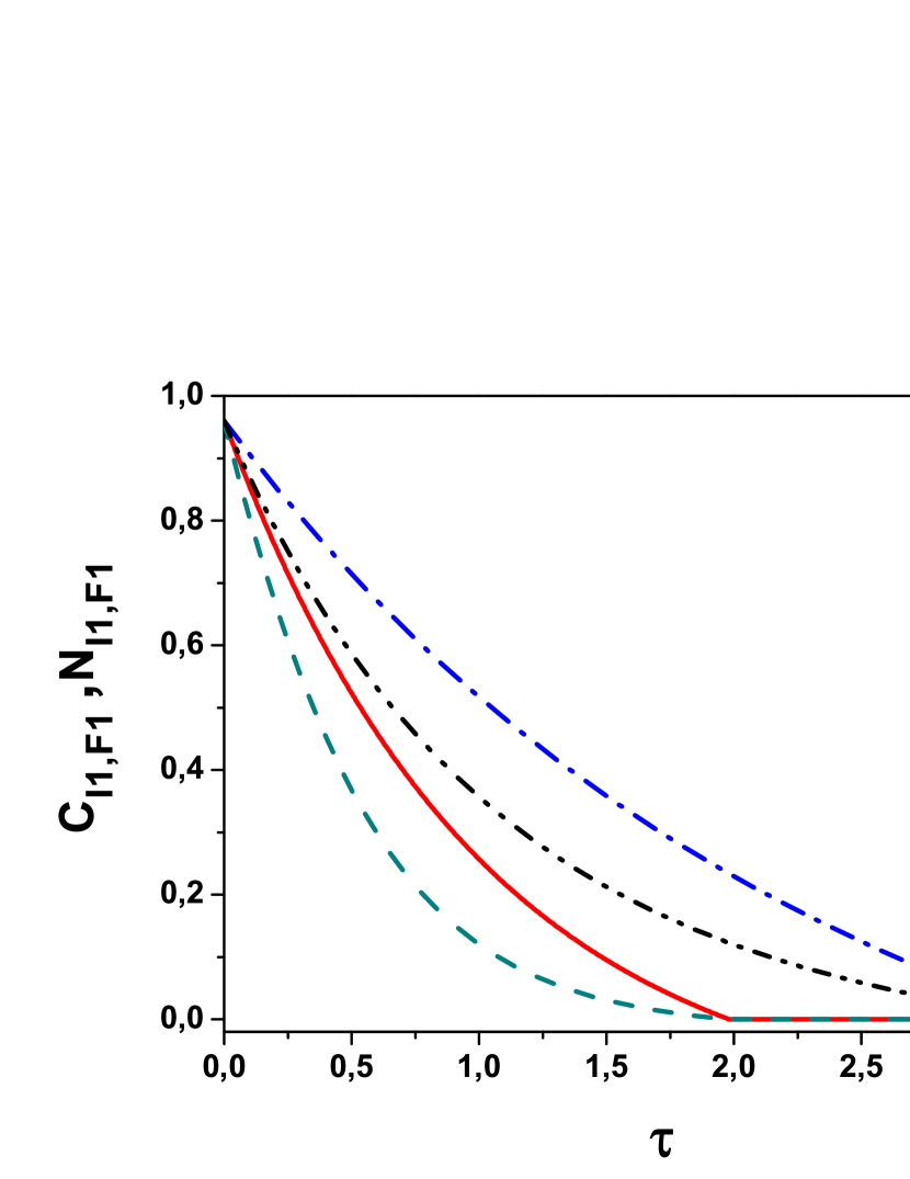
(a)

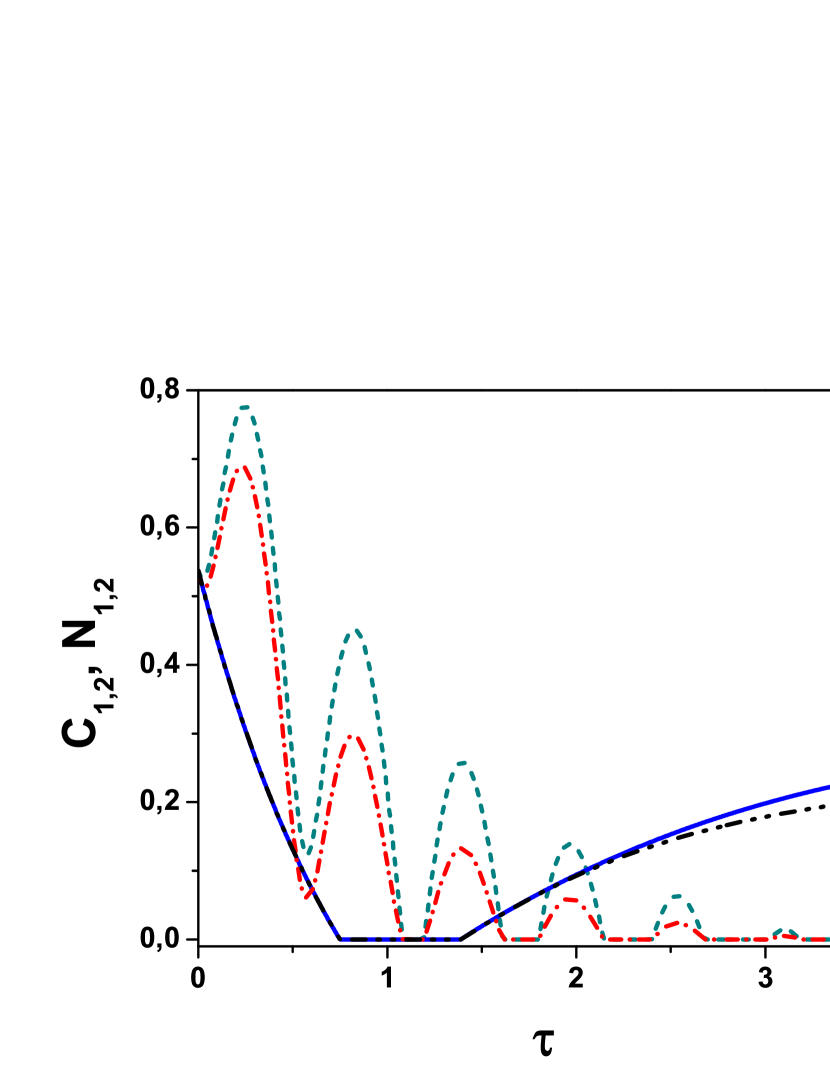
(b)

Figure 1: (a) Concurrence and negativity for models $F1$ and $I1$ (Hamiltonians (2.15) and pure Bell-like initial states (2.20), $\alpha_{1}=0.6$). The solid red line is $C_{I1}$, the blue dash dot line is $C_{F1}$, the green dash line is $N_{I1}$ and the black dash dot dot line is $N_{F1}$. Observe the ESD phenomenon and that $C_{M1}=N_{M1}=0,\;\tau=\tau_{ESD},\;C_{M1}>N_{M1},\;\tau<\tau_{ESD},\;M=I,F$, cf. (2.31) – (2.32). (b) Concurrence and negativity for the models $C1$ and $C2$ (Hamiltonian (2.13) and Bell-like pure initial states (2.20) and (2.21) with $\alpha:=\alpha_{1}=\alpha_{2}=0.96$) and the same model parameters ($\Gamma$-s in (3.12)). The green short dash line is $C_{C1}$, the red short dash dot line is $N_{C1}$. Multiple alternating ESD and ESB with positive minimum $\tau_{ESD}$ and finite maximum $\tau_{ESD}$. The blue solid line is $C_{C2}$, the black dash dot dot line is $N_{C2}$ with $0<\tau_{ESD}<\tau_{ESB}<\infty$ and $C_{C2}(\infty)=0.266$ > $N_{C2}(\infty)=0.227$.

Fig. 1(a). The figure is taken from [8]. It describes the evolution of the concurrence and the negativity corresponding to Hamiltonians (2.14) – (2.15) and the initial condition (2.20) and is given here for the comparison. It shows a simple case of the Entanglement Sudden Death (ESD) phenomenon [25, 39, 42]: the monotone $C>N$ curves for $0<\tau<\tau_{ESD}$, simultaneous ESD at $\tau=\tau_{ESD}<\infty$ and no the Entanglement Sudden Birth (ESB) phenomenon [25, 40, 42] for larger $\tau$’s (cf. (2.32) and (2.33)). This is a manifestation of the absence of the inverse flow of information from the environment to qubits pertinent to the Markovian models and preventing the ESB, although our models $I1$ and $F1$ are not Markovian in general, see (3.24) and [8]. It is worth mentioning that the results shown on Fig. 1(a) are in good qualitative agreement with certain all-optical experiments, see, e.g. [4], Fig. 21.

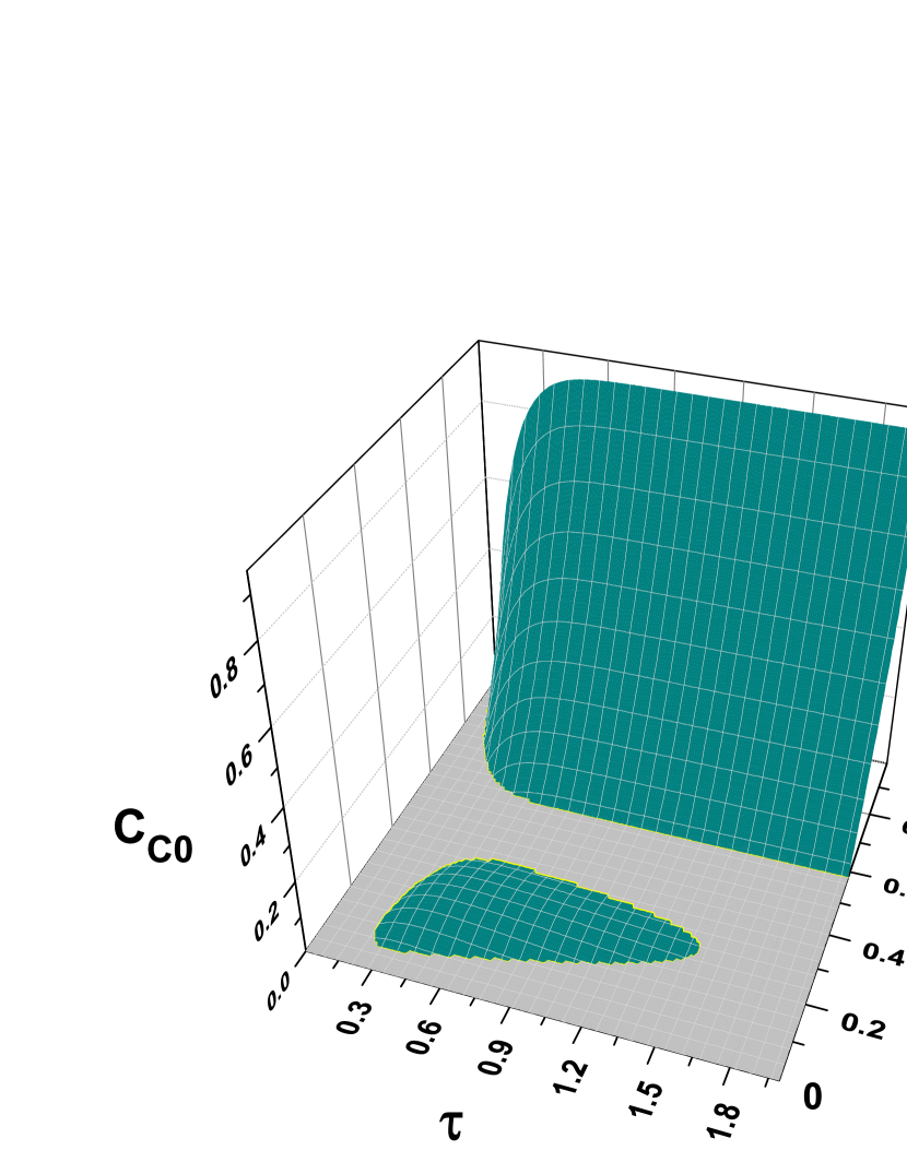
(a)

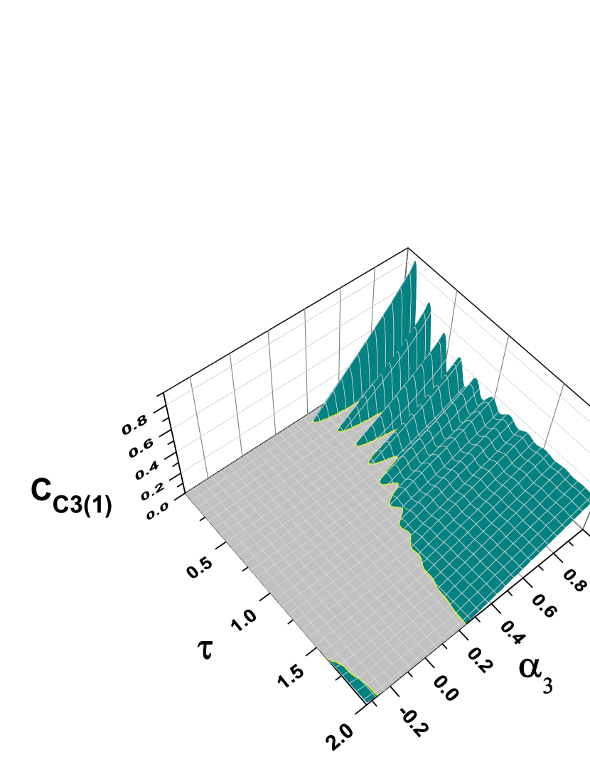
(b)

Figure 2: (a) Concurrence for the model $C0$ (the product, hence, unentangled initial states for all $\alpha_{0}\in[0,1]$). $\alpha_{0}$ close to 1 : fast growth for $\tau>\min\tau_{ESB}>0$, slow decay for large $\tau$ with zero or non-zero (trapping) at infinity. Small $\alpha_{0}$: an "island" of non-zero entanglement with $0<\tau_{ESB}<\tau_{ESD}<\infty$. (b) Concurrence for the model $C_{3(1)}$ (unentangled for $|\alpha_{3}|\leq 1/3$ initial states (2.22) and $\alpha_{1}=0.1$). Small $\alpha_{3}$: a finite "island" of non-zero entanglement. Intermediate $\alpha_{3}$: no entanglement. Close to 1 $\alpha_{3}$: $0<\tau_{ESD}^{(1)}<\tau_{ESB}^{(2)}<\tau_{ESD}^{(2)}$ finite or infinite.

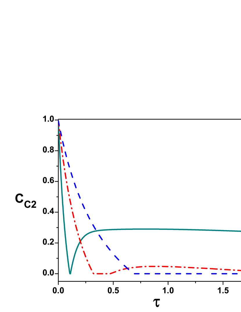
(a)

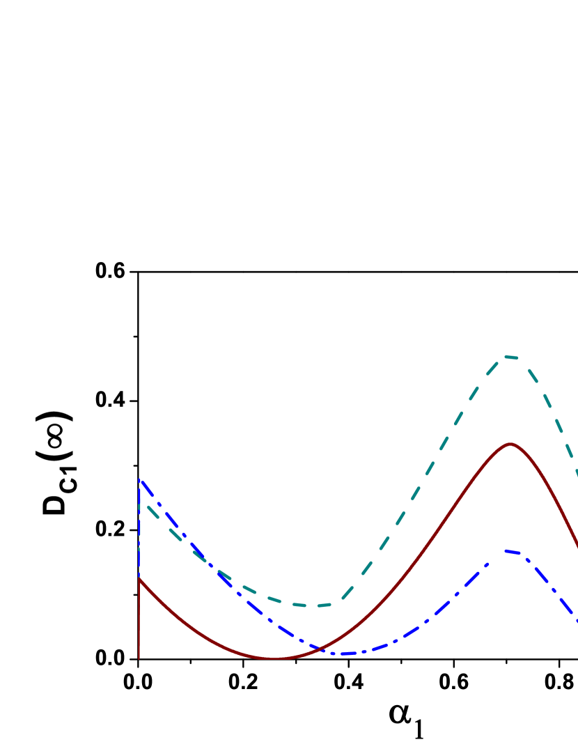
(b)

Figure 3: (a) Concurrence for the model $C2$ with $\alpha_{2}=0.67$ and various parameters ($E$ and $\gamma$) of the Lorenzian density of states of the environment (3.25). The green solid line with quite close $\tau_{ESD}$ and $\tau_{ESB}$ corresponds to $\gamma=0.15,E=1.1$, the green arrow indicates $C_{C2}(\infty)=0.071$, i.e., the entanglement trapping. The red dash dot line corresponds to $\gamma=0.33,E=1.3$ with $0<\tau^{(1)}_{ESD}<\tau_{ESB}<\tau^{(2)}_{ESD}<\infty$. The blue dash line corresponds to $\gamma=0.33,\;E=1.5$ and displays the monotone decrease from the initial value to zero at $\tau_{ESB}<\infty.$ (b) Discord at infinity for the model $C1$ as a function of the entanglement parameter $\alpha_{1}$ in (2.20) for various parameters $E$ and $\gamma$ of (3.25). The green dash line corresponds to $\;\gamma=0.2,\;E=0.5$, the blue dash dot line corresponds to $\;\gamma=0.3,\;E=1.5$ and the brown solid line corresponds to the "flat" density of states (3.23). $D_{C1}(\infty)=0$ only in the last case and only for $\alpha_{1}=0.5\sqrt{2\pm\sqrt{3}}$.

Fig. 1(b). Unlike the models $I1$ and $F1$ of Fig. 1(a) displaying a single ESD and no ESB, here, i.e., for the model $C1$ (common reservoir and the pure initial conditions (2.20)) we have multiple ESD’s and ESB’s. This is a manifestation of the backaction of the environment in the non Markovian dynamics of entanglement, resulting in our case from the indirect interaction (dynamical correlations) between the qubits via the common reservoir. Note the interplay between the behavior of $C_{C1}$ and $N_{C1}$: $C_{C1}>N_{C1}$ in the "life" periods and $C_{C1}=N_{C1}=0$ in the "death" periods (cf. (2.32) and (2.33)) with the coinciding death and birth moments. Passing from the initial conditions (2.20) to the looking quite similar initial condition (2.21), we get a different behavior of the concurrence $C_{C2}$. Here we have just one ESD and one ESB with the subsequent positive values up to a certain positive value of $C_{C1}$ at infinity. This behavior is known as the entanglement trapping, see e.g. [25] for an analogous behavior in the model with a bosonic environment.

Fig. 2 shows the behavior of the concurrence for the cases where the initial state of two qubits can be unentangled (the initial state (2.19) of Fig. 2(a) is unentangled for all $\alpha_{0}\in[0,1]$ and the initial state (2.22) of Fig. 2(b) is unentangled for $|\alpha_{3}|<1/3$). We see that in all these cases the entanglement is absent during a certain initial period ($\min\tau_{ESD}=0$), then it appears at some $\tau_{ESB}>0$ and displays the various types of behavior: fast and slow initial growth, multiple ESB’s and ESD’s and subsequent decay and vanishing either at finite moment or at infinity (hence, the trapping again). The figure demonstrates the role of dynamical correlations between the qubits via the common environment in the "producing" of the entanglement. Note that for the models of independent qubits with Hamiltonians (2.14) and (2.15), hence, without dynamical correlations, and with the same initial conditions ((2.19) or (2.22)) the concurrence is identically zero, i.e., the entanglement is absent [8]. The same is true for certain bosonic environment [25, 26].

Fig. 3 demonstrates the role of the density of states of reservoir (the Lorentzian (3.25) in our case). It follows from Fig. 3(a) that by varying the parameters ($E,\gamma$) of the density of states, we can obtain the behavior similar that on Fig. 1(a) (red solid line), Fig. 1(b) (the blue solid line) and a "new" behavior (the green solid line) with the very close $\tau_{ESB}$ and $\tau_{ESB}$ resembling a cusp in the time scale of the figure. On the other hand, according to Fig. 3(b), the behavior of the quantum discord at infinity as a function of the entanglement parameter $\alpha_{1}$ in (2.20) is qualitatively similar for all considered values of ($E,\gamma$). There are, however, two special points $\alpha_{1}=\sqrt{2\pm\sqrt{3}}/2$ where the discord is zero. It is widely believed that the cases where the discord vanishes are rather rare comparing with those for the concurrence [5, 25]. In our case this happens for the indicated values of $E,\gamma$ and $\alpha_{1}$ and for the flat density of states (3.23), where the corresponding reduced density matrix is the "uniform" state $\rho(E,\infty)=4^{-1}\mathrm{diag}(1,1,1,1)$ for which the discord is zero.

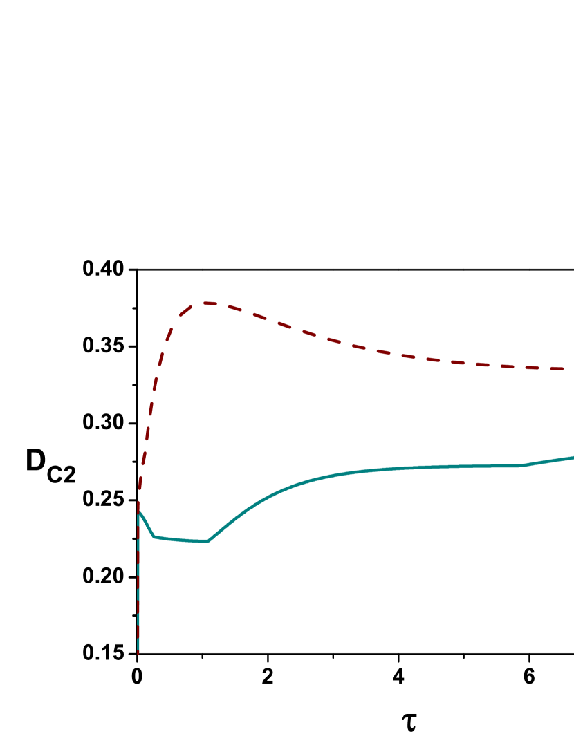
(a)

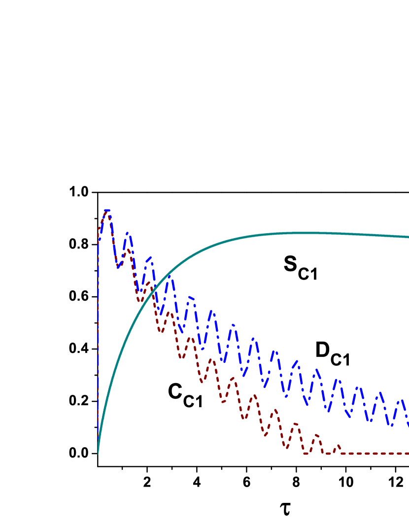
(b)

Figure 4: (a) The discord $D_{C2}$ as a function of $\tau$ for $\alpha_{2}=0.2$ where $D_{C2}(0)=0.242$. The solid green line is $D_{C2}$ with $\gamma=0.8,E=2$, the green arrow indicates $D_{C2}(\infty)=0.295$. The brown dash line is $D_{C2}$ for the flat density of states (3.23), the brown arrow indicates $D_{C2}(\infty)=0.333$. Both curves are not monotone. (b) The model $C1$ with $\alpha_{1}=1/2$. The brown short dash line is the concurrence $C_{C1},\;C_{C1}(0)=0.866,\;C_{C1}(\infty)=0$, the blue dash dot line is the discord $D_{C1},\;D_{C1}(0)=0.811,\;D_{C1}(\infty)=0.039$ (blue arrow, the discord freezing) and the green solid line is the entropy $S_{C1},\;S_{C1}(0)=0,\;S_{C1}(\infty)=0.791$ (green arrow). The concurrence decreases with oscillations to zero at a certain moment (ESD) with two ESB and two ESD in between.

Fig. 4(a) illustrates the mentioned above point on the rarity of cases where the discord vanishes. Here the discord never vanishes and the lower plot is rather structured, containing, in particular, an almost flat segment, known as the discord freezing [5, 25]. Fig. 4(b) displays the three discussed in Section 2.4 quantifiers of quantum coherence (the concurrence, the quantum discord and the entropy) with a quite structured behavior. Here the discord decreases with oscillations tending to a non zero value at infinity. The concurrence oscillate as well with similar amplitude and frequency but becomes zero at a finite moment with several ESD and ESB before. Note that the corresponding value of $\alpha_{1}$ is 1/2, but it can be shown that the analogous behavior of the concurrence holds for all $\alpha_{1}\in(0,1)$ except $\alpha_{1}=2^{-1/2}$, where the concurrence is monotone. The entropy varies regularly from zero at zero (pure initial state) to a non zero value at infinity but is not monotone. This has to be compared with the exact results of [25, 27] obtained for a particular solution of the spin boson model for two qubits with the common environment, where the entropy of the model also oscillates in time and the amplitude of oscillations is even considerably larger than that of the concurrence.

4 Large-$N$ behavior of the general reduced density matrix

In this section we will prove a general version of our basic formulas (3.1) and (4.17) – (3.9). Namely, we consider a $pN\times pN$ analog

$$H_{\mathcal{S\cup E}}=H_{\mathcal{S}}\otimes\mathbf{1}_{\mathcal{E}}+\mathbf{1}_{\mathcal{S}}\otimes M_{N}+Q_{\mathcal{S}}\otimes W_{N},$$ (4.1)

of the $4N\times 4N$ Hamiltonian (2.13), where now $H_{\mathcal{S}}$ and $Q_{\mathcal{S}}$ are $p\times p$ hermitian matrices not necessarily given by (2.6) and (2.8) for $p=4$. We note that the corresponding assertions as well as their proofs are generalizations of those for the deformed semicircle law (DSCL) of random matrix theory, see [32], Sections 2.2 and 18.3.

We will use the Greek indices varying from $1$ to $p$ to label the states of the systems and the Latin indices varying from $1$ to $N$ to label the states of the environment. Besides, we will not indicate as a rule the dependence on $N$ of the many matrices below. Hence, we write the$\ pN\times pN$ and $p\times p$ density matrices of (2.1) and (2.3) as

$$\rho_{\mathcal{S\cup E}}(t)=\{\rho_{\alpha j,\beta k}(t)\}_{\alpha,\beta=1,j,k=1}^{p,N},$$ (4.2)

$$\;\rho_{\mathcal{S}}(t)=\{\rho_{\alpha\beta}(t)\}_{\alpha,\beta=1}^{p},\;\;\rho_{\alpha\beta}(t)=N^{-1}\sum_{j=1}^{N}\rho_{\alpha j,\beta j}(t),\;\alpha,\beta=1,...,p.$$ (4.3)

Since the probability law (2.10) is unitary invariant, we can assume without loss of generality that the hermitian matrix $M_{N}$ (the environment Hamiltonian) in (4.1) is diagonal

$$M_{N}=\{\delta_{jk}E_{N}^{(k)}\}_{j,k=1}^{N},$$ (4.4)

i.e., we can use the orthonormal basis of its eigenvectors as the basis in the state space of the environment.

It follows then from (2.1) – (2.3) and (2.16) that the matrix form of the channel superoperator (2.4) is

$$(\rho_{\mathcal{S}}(t))_{\alpha\beta}=\sum_{\gamma,\delta=1}^{p}\Phi_{\alpha\beta\gamma\delta}^{(k)}(t)(\rho_{\mathcal{S}}(0))_{\gamma\delta},$$ (4.5)

where

$$\Phi_{\alpha\beta\gamma\delta}^{(k)}(t)=\sum_{j=1}^{N}U_{\alpha j,\gamma k}(-t)U_{\delta k,\beta j}(t),$$ (4.6)

and

$$U(\pm t)=e^{\pm itH}=\{U_{\alpha j,\beta k}(\pm t)\}_{\alpha,\beta=1,j,k=1}^{p,N}.$$ (4.7)

Result 1. Consider the Hamiltonian (4.1) where $H_{\mathcal{S}}$ and $Q_{\mathcal{S}}$ are $p\times p$ arbitrary $N$-independent hermitian matrices, $M_{N}$ is a hermitian $N\times N$ matrix satisfying (2.9) and (2.17) and $W_{N}$ is given by (2.10) – (2.11). Then we have for the entries (4.3) of the reduced density matrix (4.3)

$$\mathbf{Var}\{\rho_{\alpha\beta}(t)\}=\mathbf{E}\{|\rho_{\alpha\beta}(t)|^{2}\}-|\mathbf{E}\{\rho_{\alpha\beta}(t)\}|^{2}$$

$$\hskip 71.13188pt\leq Ct^{2}\mathrm{Tr}Q_{\mathcal{S}}^{2}/N,\;C=4p^{2},\;\alpha,\beta=1,...,p.$$ (4.8)

Proof of Result 1. We view every $\rho_{\alpha\beta}(t)$ of (4.5) – (4.7) as a function of the Gaussian random variables $\{W_{ab}\}_{a,b=1}^{N}$ of (2.10) – (2.11) and use the Poincaré inequality (see [32], Proposition 2.1.6) according to which we have for any differentiable and polynomially bounded function $\varphi$ of the collection $\{W_{ab}\}_{a,b=1}^{N}$:

$$\mathbf{Var}\{\varphi\}=\mathbf{E}\left\{\left|\varphi\right|^{2}\right\}-|\mathbf{E}\left\{\varphi\right\}|^{2}\leq N^{-1}\sum_{a,b=1}^{N}\mathbf{E}\left\{\left|\frac{\partial\varphi}{\partial W_{ab}}\right|^{2}\right\}.$$ (4.9)

To find the derivatives of $\varphi=\rho_{\alpha\beta}(t)$ with respect to $W_{ab}$, we use the Duhamel formula

$$\frac{d}{dx}e^{A(x)}=\int_{0}^{1}dse^{(1-s)A(x)}\frac{d}{dx}A(x)e^{sA(x)}$$ (4.10)

valid for any differentiable matrix-function $A$ of $x$. In our case $A=itH_{\mathcal{A}\cup\mathcal{E}}$ of (4.1) viewed as a function of $W_{ab}$ for a given pair $(a,b)$. By using (4.1), (4.7), (4.9) and (4.10), we obtain

$$\frac{\partial}{\partial W_{ab}}U_{\alpha j,\beta k}(\pm t)=\pm i\int_{0}^{t}ds\sum_{\alpha^{\prime},\beta^{\prime}=1}^{p}U_{\alpha j,\alpha^{\prime}a}(\pm(t-s))Q_{\alpha^{\prime}\beta^{\prime}}U_{\beta^{\prime}b,\beta k}(\pm s).$$ (4.11)

and we omit the subindex $\mathcal{S}$  in $Q$ here and often below. This, (2.1), (2.3) and (4.1) yield

$$\frac{\partial}{\partial W_{ab}}\rho_{\alpha\beta}(t)=T^{(1)}_{ab}+T^{(2)}_{ab},$$ (4.12)

where

$$T_{ab}^{(1)} = -\int_{0}^{t}ds\sum_{\alpha^{\prime},\gamma,\gamma^{\prime},\delta=1}^{p}\sum_{j=1}^{N}U_{\alpha j,\alpha^{\prime}a}(-(t-s))Q_{\alpha^{\prime}\gamma^{\prime}}U_{\gamma^{\prime}b,\gamma k}(-s)\rho_{\gamma\delta}(0)U_{\delta k,\beta j}(t),$$

$$T_{ab}^{(2)} = -\int_{0}^{t}ds\sum_{\beta^{\prime},\gamma,\delta,\delta^{\prime}=1}^{p}\sum_{j=1}^{N}U_{\alpha j,\gamma k}(-t)\rho_{\gamma\delta}(0)U_{\delta k,\delta^{\prime}a}(t-s)Q_{\delta^{\prime}\beta^{\prime}}U_{\beta^{\prime}b,\beta j}(s).$$ (4.13)

We have then by (4.9)

$$\mathbf{Var}\{\rho_{\alpha\beta}(t)\} \leq N^{-1}\sum_{a,b=1}^{N}\mathbf{E}\left\{\left|T_{ab}^{(1)}+T_{ab}^{(2)}\right|^{2}\right\}$$ (4.14)

$$\leq 2N^{-1}\mathbf{E}\left\{\sum_{a,b=1}^{N}\left|T_{ab}^{(1)}\right|^{2}\right\}+2N^{-1}\mathbf{E}\left\{\sum_{a,b=1}^{N}\left|T_{ab}^{(2)}\right|^{2}\right\}.$$

The first sum on the right of (4.14) is by (4.13)

$$\sum_{a,b=1}^{N}\left|T_{ab}^{(1)}\right|^{2} = \sum_{a,b=1}^{N}$$

$$\times\left|\int_{0}^{t}ds\sum_{\alpha^{\prime},\gamma,\gamma^{\prime},\delta=1}^{p}\sum_{j=1}^{N}U_{\alpha j,\alpha^{\prime}a}(-t+s)Q_{\alpha^{\prime}\gamma^{\prime}}U_{\gamma^{\prime}b,\gamma k}(-s)\rho_{\gamma\delta}(0)U_{\delta k,\beta j}(t)\right|^{2}.$$

By applying Schwarz inequality to the sum over $\alpha^{\prime},\gamma,\gamma^{\prime},\delta$ and to the integral over $t$, we obtain

$$\sum_{a,b=1}^{N}\left|T_{ab}^{(1)}\right|^{2} \leq t\sum_{\alpha^{\prime},\gamma^{\prime}=1}^{p}|Q_{\alpha^{\prime}\gamma^{\prime}}|^{2}\sum_{\gamma,\delta=1}^{p}|\rho_{\gamma\delta}(0)|^{2}\int_{0}^{t}ds\sum_{\gamma^{\prime},b=1}^{p,N}|U_{\gamma^{\prime}b,\gamma k}(-s)|^{2}$$ (4.15)

$$\times\sum_{\gamma,\delta=1}^{p}\sum_{j_{1},j_{2}=1}^{N}\sum_{\alpha^{\prime},a=1}^{p,N}U_{\alpha j_{1},\alpha^{\prime}a}(-(t-s))U_{\alpha j_{2},\alpha^{\prime}a}^{\ast}(-(t-s))U_{\delta k,\beta j_{1}}(t)U_{\delta k,\beta j_{2}}^{\ast}(t),$$

where the symbol "$\ast$" denotes the complex conjugate.

Recalling now that $U(t)$ is unitary group, hence, $U_{\alpha j,\beta k}^{\ast}(t)=U_{\beta k,\alpha j}^{\ast}(-t)$ and for any $\alpha_{1},\alpha_{2}$, $j_{1},j_{2},s_{1},s_{2}$

$$\sum_{\alpha\text{ }^{\prime},a=1}^{p,N}U_{\alpha_{1}j_{1},\alpha^{\prime}a}(s_{1})U_{\alpha_{2}j_{2},\alpha^{\prime}a}^{\ast}(s_{2}) = U_{\alpha_{1}j_{1},\alpha_{2}j_{2}}(s_{1}-s_{2}),\;$$ (4.16)

$$U_{\alpha_{1}j_{1},\alpha_{2}j_{2}}(0) = \delta_{\alpha_{1}\alpha_{2}}\delta_{j_{1}j_{2}},$$

we obtain that the sum over $(\alpha^{\prime},\gamma^{\prime})$ is $\mathrm{Tr}Q^{2}$, the first sum over $(\gamma,\delta)$ is $\mathrm{Tr}\rho^{2}(0)\leq 1$, the sum over ($\gamma^{\prime},b$)  is 1 by (4.16), the sum over ($\alpha^{\prime},a)$ is $\delta_{j_{1}j_{2}}$ again by (4.16) and then the sum over $j=j_{1}=j_{2}$ is bounded by 1 also by (4.16) and the second sum over $(\gamma,\delta)$ is $p^{2}$. We conclude that

$$\sum_{a,b=1}^{N}\left|T_{ab}^{(1)}\right|^{2}\leq p^{2}t^{2}\mathrm{Tr}_{\mathcal{S}}Q^{2}_{\mathcal{S}}.$$

An analogous argument yields the same bound for the second sum in (4.14) and we obtain (4.8). $\blacksquare$

Result 2. In the setting of Result 1 above we have uniformly in $t$ varying on any compact interval of $[0,\infty)$:

$$\rho(E,t) = \lim_{N\rightarrow\infty}\mathbf{E}\{\rho_{S}(t)\}$$ (4.17)

$$= -\frac{1}{(2\pi i)^{2}}\int_{-\infty-i\varepsilon}^{\infty-i\varepsilon}dz_{1}\int_{-\infty+i\varepsilon}^{\infty+i\varepsilon}dz_{2}e^{i(z_{1}-z_{2})t}F(E,z_{1},z_{2}),$$

where $F$ solves the linear $p\times p$ matrix equation

$$F(E,z_{1},z_{2})=F_{0}(E,z_{1},z_{2})$$

$$+\int_{-\infty}^{\infty}G(E^{\prime},z_{2})Q_{\mathcal{S}}F(E,z_{1},z_{2})Q_{\mathcal{S}}G(E^{\prime},z_{1})\nu_{0}(E^{\prime})dE^{\prime}$$ (4.18)

with the density of states of the environment $\nu_{0}$ defined in (2.9),

$$F_{0}(E,z_{1},z_{2})=G(E,z_{2})\rho_{\mathcal{S}}(0)G(E,z_{1}),$$ (4.19)

$$G(E,z)=(E+H_{\mathcal{S}}-z-Q_{\mathcal{S}}\mathsf{G}(z)Q_{\mathcal{S}})^{-1}$$ (4.20)

and $\mathsf{G}(z)$ solving uniquely the non-linear $p\times p$ matrix equation

$$\mathsf{G}(z)=\int_{-\infty}^{\infty}(E^{\prime}+H_{\mathcal{S}}-z-Q_{\mathcal{S}}\mathsf{G}(z)Q_{\mathcal{S}})^{-1}\nu_{0}(E^{\prime})dE^{\prime}$$ (4.21)

in the class of $p\times p$ analytic in $\mathbb{C}\setminus\mathbb{R}$ matrix functions such that

$$\Im\mathsf{G}(z)\Im z>0,\;\Im z\neq 0,\;\sup_{y\geq 1}y||\mathsf{G}(iy)||\leq\infty.$$ (4.22)

Proof of Result 2. This proof is more involved than that of Result 1. We will start with the asymptotic analysis of

$$\overline{U}_{\alpha j,\beta k}(t)=\mathbf{E}\{U_{\alpha j,\beta k}(t)\},$$ (4.23)

i.e., the first moment of the evolution operator (4.7), since the moment is necessary for the asymptotic analysis of the second moment, i.e., according to (4.6), of

$$\mathbf{E}\{\Phi_{\alpha\beta\gamma\delta}^{(k)}(t)\}=\mathbf{E}\left\{\sum_{j=1}^{N}U_{\alpha j,\gamma k}(-t)\}U_{\delta k,\beta j}(t)\}\right\}.$$ (4.24)

which results in (4.18) – (4.21). Besides, the asymptotic analysis of (4.23) includes several important technical steps which are also used in the analysis of (4.24), but are less tedious and more transparent for (4.23) than for (4.24).

Asymptotic analysis of (4.23). It is convenient to pass from the evolution operator (4.7) of the $pN\times pN$ hermitian matrix $H_{\mathcal{S\cup E}}$ of (4.1) to its resolvent

$$G_{H_{\mathcal{S\cup E}}}(z)=(H_{\mathcal{S\cup E}}-z)^{-1}=\{G_{\alpha j,\beta k}(z)\}_{\alpha,\beta,j,k=1}^{pN},\;\Im z\neq 0$$ (4.25)

by using the formulas

$$G_{H_{\mathcal{S\cup E}}}(z)=\pm i\int_{0}^{\infty}dte^{\mp itz}U_{H_{\mathcal{S\cup E}}}(\pm t),\;\Im z\lessgtr 0.$$ (4.26)

Given the resolvent we obtain the evolution operator via the inversion formula

$$U_{H_{\mathcal{S\cup E}}}(\pm t)=\mp\frac{1}{2\pi i}\int_{-\infty\pm i\varepsilon}^{\infty\pm i\varepsilon}dte^{\pm itz}G_{H_{\mathcal{S\cup E}}}(z),$$ (4.27)

where the integral is understood in the Cauchy sense at infinity.

In view of the above formulas is suffices to find an asymptotic form of the expectation (the first moment)

$$\overline{G}_{H_{\mathcal{S\cup E}}}(z)=\mathbf{E}\{G_{H_{\mathcal{S\cup E}}}(z)\}=\{\overline{G}_{\alpha j,\beta k}(z)\}_{\alpha,\beta=1,j,k=1}^{p,N},\;\Im z\neq 0.$$ (4.28)

of the resolvent (4.25).

To this end we will use an extension of the tools of random matrix theory as they presented in [32] and used there to derive the so called deformed semicircle law for Gaussian random matrices, the "scalar" case of $p=1$ and then, in [22], to deal with the one-qubit case of $p=2$ for (4.1).

Denote for brevity

$$H_{\mathcal{S\cup E}}=H=H^{(0)}+H^{(1)},\;$$

$$H^{(0)}=H_{\mathcal{S}}\times 1_{\mathcal{E}}+1_{\mathcal{S}}\times M_{N},\;H_{1}=H_{\mathcal{SE}}=vQ_{\mathcal{S}}\times W_{N}$$ (4.29)

in (4.1) (recall that $H_{\mathcal{S}}$ and $Q_{\mathcal{S}}$ are now arbitrary $p\times p$ hermitian matrices, i.e., not necessarily given by (2.6) and (2.8)). Set

$$G(z)=(H-z)^{-1},\;G^{(0)}(z)=(H^{(0)}-z)^{-1},\;\Im z\neq 0$$

and use the resolvent identity

$$G(z)=G^{(0)}(z)-G(z)H^{(1)}G^{(0)}(z)$$ (4.30)

to write

$$\overline{G}_{\alpha j,\beta k}=G_{\alpha j,\beta k}^{(0)}-\sum_{\alpha^{\prime},\beta^{\prime}=1,}^{p}\sum_{j^{\prime},k^{\prime}=1}^{N}\mathbf{E}\{G_{\alpha j,\alpha^{\prime}j^{\prime}}Q_{\alpha^{\prime}\beta^{\prime}}W_{j^{\prime}k^{\prime}}\}G_{\beta^{\prime}k^{\prime},\beta k}^{(0)},$$ (4.31)

where we omit the subindex $\mathcal{S}$ in $Q_{\mathcal{S}}$ and the argument $z$ in $G$.

To proceed we will use the Gaussian differentiation formula, according to which if $\{W_{ab}\}_{a,b=1}^{N}$ is the collection of complex Gaussian random variables (2.10) – (2.11) and $\varphi$ is a differentiable and polynomially bounded function of the collection, then (see [32], Section 2.1)

$$\mathbf{E}\{W_{ab}\varphi\}=N^{-1}\mathbf{E}\left\{\frac{\partial\varphi}{\partial W_{ba}}\right\},\;a,b=1,...,N.$$ (4.32)

Viewing $G_{\alpha j,\alpha^{\prime}j^{\prime}}$ as function of a particular $W_{ab}$ and using the formula (cf. (4.11)),

$$\frac{\partial}{\partial W_{ab}}G_{\rho r,\sigma s}=-\sum_{\rho^{\prime},\sigma^{\prime}=1}^{p}G_{\rho r,\rho^{\prime}a}Q_{\rho^{\prime}\sigma^{\prime}}G_{\sigma^{\prime}b,\sigma s},$$ (4.33)

which follows easily from the resolvent identity (4.30) (cf. (4.10)), we obtain from (4.31)

$$\overline{G}_{\alpha j,\beta k} = G_{\alpha j,\beta k}^{(0)}-N^{-1}\sum_{\alpha^{\prime},\beta^{\prime}=1,j^{\prime},k^{\prime}=1}^{p,N}\mathbf{E}\left\{\frac{\partial}{\partial W_{k^{\prime}j^{\prime}}}G_{\alpha j,\alpha^{\prime}j^{\prime}}\right\}Q_{\alpha^{\prime}\beta^{\prime}}G_{\beta^{\prime}k^{\prime},\beta k}^{(0)}$$ (4.34)

$$= G_{\alpha j,\beta k}^{(0)}+\sum_{\alpha^{\prime},\beta^{\prime}=1}^{p}\sum_{j^{\prime}=1}^{N}\mathbf{E}\left\{G_{\alpha j,\alpha^{\prime}j^{\prime}}(g_{Q})_{\alpha^{\prime}\beta^{\prime}}\right\}G_{\beta^{\prime}j^{\prime},\beta k}^{(0)},$$

where

$$g_{Q}=QgQ,\;\;g = N^{-1}\mathrm{Tr}_{\mathcal{E}}G=\{g_{\gamma\delta}\}_{\gamma,\delta=1}^{p},\;$$

$$g_{\gamma\delta} = N^{-1}\sum_{k^{\prime}=1}^{N}G_{\gamma k^{\prime},\delta k^{\prime}}.$$ (4.35)

Writing

$$g=\overline{g}+g^{\circ},\;\mathbf{E}\left\{g^{\circ}\right\}=0,$$ (4.36)

we present (4.34) in the compact matrix form

$$\overline{G}=G^{(0)}+\overline{G}(\overline{g}_{Q}\times\mathbf{1}_{\mathcal{E}})G^{(0)}+R^{(1)}G^{(0)}$$ (4.37)

with

$$R^{(1)}=\mathbf{E}\left\{G(g_{Q}^{\circ}\times\mathbf{1}_{\mathcal{E}})\right\}.$$ (4.38)

Denote $\{\lambda_{\tau t}\}_{\tau,t=1}^{pN}$ and $\{\Psi_{\tau t}\}_{\tau,t=1}^{pN}$ the eigenvalues (possibly repeating) and orthonormal eigenvectors of $pN\times pN$ matrix $H$ of (4.29). It follows then from the spectral theorem that

$$G=(H-z)^{-1}=\sum_{\tau,t=1}^{pN}\frac{1}{\lambda_{\tau t}-z}P_{\tau t},$$ (4.39)

where $P_{\tau t}$ is the orthogonal projection on $\Psi_{\tau t}$.

Writing further for any matrix $A$

$$\Im A:=(A-A^{+})/2i,$$ (4.40)

where $A^{+}$ is the hermitian conjugate of $A$ and for any hermitian matrices $A$ and $B$

$$A>B$$

if $A-B$ is positive definite, we have from (4.39)

$$\Im G(z)/\Im z>0,\;\Im z\neq 0.$$

The same inequality holds for $\overline{G}$, $\overline{g}=N^{-1}\mathrm{Tr}_{\mathcal{E}}\overline{G}$ and $\overline{g}_{Q}$ of (4.35). This implies the bound

$$\Im(H^{(0)}-z-\overline{g}_{Q})/\Im z=-(\mathbf{1}_{\mathcal{S}}+\Im Q\overline{g}Q/\Im z)\times\mathbf{1}_{\mathcal{E}}<-\eta\mathbf{1}_{\mathcal{S\cup E}},$$ (4.41)

with an $N$-independent $\eta>0$ and

$$|\Im z|\geq\eta>0.$$ (4.42)

Hence, the $pN\times pN$ matrix $H^{(0)}-z-\overline{g}_{Q}(z)\times\mathbf{1}_{\mathcal{E}}$ is invertible uniformly in $N$ and (4.37) is equivalent to

$$\overline{G}(z)=G^{(0)}(z_{Q})+R^{(1)}(z)G^{(0)}(z_{Q}),\;z_{Q}=z\mathbf{1}_{\mathcal{S}}+\overline{g}_{Q}(z).$$ (4.43)

Note now that $H^{(0)}$ of (4.29) admits the separation of variables, hence, in its spectral representation (see (4.39)) $\lambda_{\tau t}=\varepsilon_{\tau}+E_{t}$, $\Psi_{\tau t}=\psi_{\tau}\otimes\Psi_{t}$, where $\{\varepsilon_{\tau}\}_{\tau=1}^{p}$ and $\{E_{t}\}_{t=1}^{N}$ are the eigenvalues   and $\{\psi_{\tau}\}_{\tau=1}^{p}$ and $\{\Psi_{t}\}_{t=1}^{N}$ are the eigenvectors of $H_{\mathcal{S}}$ and $H_{\mathcal{E}}=M_{N}$. Besides, $M_{N}$ is diagonal, see (4.4), hence, $\Psi_{t}=\{\delta_{jt}\}_{j=1}^{N}$ and we have from (4.39)

$$G_{\alpha j,\beta k}^{(0)}(z) = \delta_{jk}G_{\alpha\beta}^{\mathcal{S}}(z-E_{k}),\;$$

$$G^{\mathcal{S}}(z) = (H_{\mathcal{S}}-z)^{-1}=\{G_{\alpha\beta}^{\mathcal{S}}(z)\}_{\alpha,\beta=1}^{p}.$$ (4.44)

This allows us to write (4.43) as

$$\overline{G}_{\alpha j,\beta k}(z)=\delta_{jk}G_{\alpha\beta}^{\mathcal{S}}(z_{Q}-E_{j})+\sum_{\gamma=1}^{p}R^{(1)}_{\alpha j,\gamma k}G_{\gamma\beta}^{\mathcal{S}}(z_{Q}-E_{j}),$$ (4.45)

and, combining (2.9), (4.35) and (4.45), we get

$$\overline{g}(z)=\int G^{\mathcal{S}}(z_{Q}-E)\nu_{N}(E)dE+r(z),$$ (4.46)

where

$$r_{\alpha\beta}(z)=N^{-1}\sum_{\gamma=1}^{p}\sum_{k=1}^{N}\mathbf{E}\left\{G_{\mathcal{\alpha}k,\gamma k}(z)((Qg^{\circ}Q)G^{\mathcal{S}}(z_{Q}-E_{k}))_{\gamma\beta}\right\}.$$ (4.47)

It follows from (4.39) and (4.41) that

$$|G_{j\alpha,j\beta}(z)|\leq||G(z)||\leq|\Im z|^{-1},\;||G^{\mathcal{S}}(z_{Q}-E_{k})||\leq|\Im z|^{-1}.$$ (4.48)

This and the bound

$$|Q_{\alpha,\beta}|\leq||Q||,\;\alpha,\beta=1,...,p$$ (4.49)

imply

$$|r_{\alpha\beta}(z)|\leq\frac{p^{2}||Q||^{2}}{|\Im z|^{2}}\sum_{\gamma,\delta=1}^{p}\mathbf{E\{}|g_{\gamma\delta}^{\circ}|\}\leq\frac{p^{2}||Q||^{2}}{|\Im z|^{2}}\sum_{\gamma,\delta=1}^{p}\mathbf{Var}^{1/2}\left\{g_{\gamma\delta}\right\}.$$ (4.50)

We will bound $\mathbf{Var}\left\{g_{\gamma\delta}\right\}$ by using again the Poincaré inequality (4.9). We have by (4.33)

$$\frac{\partial g_{\gamma\delta}}{\partial W_{ab}} = -\frac{1}{N}\sum_{j=1}^{N}\sum_{\gamma^{\prime},\delta^{\prime}=1}^{p}G_{\gamma j,\gamma^{\prime}a}G_{\delta^{\prime}b,\delta j}Q_{\gamma^{\prime}\delta^{\prime}}$$ (4.51)

$$= -\frac{1}{N}\sum_{\gamma^{\prime},\delta^{\prime}=1}^{p}Q_{\gamma^{\prime}\delta^{\prime}}\left(\sum_{j=1}^{N}G_{\gamma j,\gamma^{\prime}a}G_{\delta^{\prime}b,\delta j}\right)$$

and then, by Schwarz inequality and (4.49)

$$\left|\frac{\partial g_{\gamma\delta}}{\partial W_{ab}}\right|^{2} \leq \frac{p^{2}||Q||^{2}}{N^{2}}\sum_{\gamma^{\prime},\delta^{\prime}=1}^{p}\sum_{a,b=1}^{N}\left|\sum_{j=1}^{N}G_{\gamma j,\gamma^{\prime}a}G_{\delta^{\prime}b,\delta j}\right|^{2}.$$

Plugging this into the r.h.s. of (4.9) with $\varphi=g_{\gamma\delta}$, we obtain

$$\mathbf{Var}\left\{g_{\gamma\delta}\right\}\leq\frac{p^{2}||Q||^{2}}{N^{3}}\mathrm{Tr}_{\mathcal{E}}\Gamma_{\gamma\gamma}\Gamma_{\delta\delta}^{\ast},$$

where

$$\Gamma_{\alpha\alpha}=\{(GG^{+})_{\alpha j_{1},\alpha j_{2}}\}_{j_{1},j_{2}=1}^{N}$$

is the $N\times N$ matrix and it follows from (4.39) that $||\Gamma_{\alpha\alpha}||\leq||\Im z|^{-2}$. This and the bound $|\mathrm{Tr}_{\mathcal{E}}A|\leq||A||N$ valid for any $N\times N$ matrix yield

$$\mathbf{Var}\{g_{\alpha\beta}(z)\}\leq\frac{p^{2}||Q||^{2}}{N^{2}|\Im z|^{4}}$$ (4.52)

implying together with (4.50)

$$|r_{\alpha\beta}(z)|\leq\frac{p^{3}||Q||^{3}}{N|\Im z|^{4}},\;\alpha,\beta=1,...,p.$$ (4.53)

The bound and the standard argument of random matrix theory (see [32], Chapter 2) allow us to conclude that the sequence $\{\overline{g}_{N}\}_{N}$ of $p\times p$ analytic in $\mathbb{C}\setminus\mathbb{R}$ matrix function (4.35) contains a subsequence $\{\overline{g}_{N_{n}}\}_{n}$ which converges uniformly on any compact set of $\mathbb{C}\setminus\mathbb{R}$ to a unique solution $\mathsf{G}(z)$ of the matrix functional equation (4.21) – (4.22). Hence, the whole sequence $\{\overline{g}_{N}\}_{N}$ converges uniformly on any compact set of $\mathbb{C}\setminus\mathbb{R}$ to the limit $\mathsf{G}$ solving uniquely (4.21) – (4.22).

Note that this assertion is a matrix analog of that on the so-called deformed semicircle law of random matrix theory, see [32], Chapter 2. In articular, the proof of the unique solvability of (3.9) – (4.22) repeats almost literally the corresponding proof in [32].

Consider now the expectation (4.28) of the resolvent. It it is easy to see that a slightly modified version of an argument proving (4.53) yields for the second term of (4.45) the bound coinciding with the r.h.s. of (4.53), i.e.,

$$\left|\overline{G}_{\alpha j,\beta k}(z)-\delta_{jk}G_{\alpha\beta}^{\mathcal{S}}(z_{Q}(z)-E_{k})\right|\leq\frac{p^{3}||Q||^{3}}{N|\Im z|^{4}},\;\alpha,\beta=1,...,p,\;j=1,...,N.$$ (4.54)

This bound implies for any $z$ satisfying (4.42) and all $\alpha,\beta=1,...,p<\infty$

$$\lim_{N\rightarrow\infty}\overline{G}_{\alpha j,\beta k}(z)=0,\;j\neq k,\;j,k=1,...,N,$$ (4.55)

and if $k=k_{N}\rightarrow\infty,\;N\rightarrow\infty$ and is such that (2.17) holds, then

$$G(E,z) = \lim_{N\rightarrow\infty}\overline{G}_{\alpha k_{N},\beta k_{N}}(z)=G_{\alpha\beta}^{\mathcal{S}}(Z_{Q}-E),$$

$$Z_{Q}(z) = z\mathbf{1}_{\mathcal{S}}+Q\mathsf{G}(z)Q,$$ (4.56)

where $Z_{Q}$ the $N\rightarrow\infty$ limit of the $p\times p$ matrix function $z_{Q}$ given in (4.43).

Note now that by (4.7) and (4.29)

$$\frac{d}{dt}\overline{U}_{\alpha j,\beta k}(t)=i\mathbf{E}\{(U(t)H)_{\alpha j,\beta k}\}=i\sum_{\gamma,l=1}^{p,N}\mathbf{E}\{U(t)_{\alpha j,\gamma l}H_{\gamma l,\beta k}\},$$

hence, by Schwarz inequality,

$$\left|\frac{d}{dt}\overline{U}_{\alpha j,\beta k}(t)\right|\leq\mathbf{E}^{1/2}\left\{\sum_{\gamma,l=1}^{p,N}|U(t)_{\alpha j,\gamma l}|^{2}\right\}\mathbf{E}^{1/2}\left\{\sum_{\gamma,l=1}^{p,N}|H_{\gamma l,\beta k}|^{2}\right\}.$$

The first factor on the right is bounded by 1 in view of (4.16) and according to (4.29) and (2.11) the second factor admits the bound

$$3^{1/2}\left(\sum_{\gamma=1}^{p}|H_{\gamma\beta}^{\mathcal{S}}|^{2}+|E_{k}^{(N)}|^{2}+||Q||^{2}\sum_{l=1}^{N}\mathbf{E\{}|W_{lk}|\}^{2}\right)^{1/2}$$

It follows from (2.11) that the above expression is bounded in $\alpha,\beta,j,k,N$ provided (2.17) is valid. Thus, the collection of continuous in $t$ functions $\overline{U}_{\alpha j,\beta k}:\mathbb{R}\rightarrow\mathbb{C}$ contains a subsequence $\{\overline{U}_{\alpha j^{(N)},\beta k^{(N)}}\}_{N}$ in $N$ (where ($j_{N},k_{N}$) do not necessarily depend on $N$) which converges uniformly in $t\in[0,t_{0}],\;\forall t_{0}<\infty$ to a certain continuous function. This, (4.26), (4.27) and (4.55) – (4.56) imply for any $\alpha,\beta=1,...,p$

$$\lim_{N\rightarrow\infty}\overline{U}_{\alpha j,\beta k}(t)=0,\;j\neq k,\;j,k=1,...,N,$$ (4.57)

and if $k=k^{(N)}\rightarrow\infty,\;N\rightarrow\infty$ is such that (2.17) holds, then

$$\lim_{N\rightarrow\infty}\overline{U}_{\alpha k^{(N)},\beta k^{(N)}}(t)=\frac{1}{2\pi i}\int_{-\infty-i\varepsilon}^{\infty-\varepsilon}e^{itz}G_{\alpha\beta}^{\mathcal{S}}(Z_{Q}(z)-E)dz,$$ (4.58)

where $Z_{Q}$ is defined in (4.56).

Asymptotic analysis of the channel operator. It follows from Result 1 above that it suffices to consider the expectation

$$\overline{\Phi}_{\alpha\beta\gamma\delta}^{(k)}(t)=\sum_{j=1}^{N}\mathbf{E}\{U_{\alpha j,\gamma k}(-t)U_{\delta k,\beta j}(t)\}.$$ (4.59)

of the entries (4.6) of the superoperator.

Introduce

$$\Phi_{\alpha\beta\gamma\delta}^{(k)}(t_{1},t_{2}) = \sum_{j=1}^{N}U_{\alpha j,\gamma k}(-t_{2})U_{\delta k,\beta j}(t_{1}),\;t_{1}\geq 0,\;t_{2}\geq 0,$$

$$\Phi_{\alpha\beta\gamma\delta}^{(k)}(t) = \Phi_{\alpha\beta\gamma\delta}^{(k)}(-t,t),\;t\geq 0,$$ (4.60)

and pass from the evolution operator (4.7) of the total hamiltonian $H_{\mathcal{S\cup E}}$ to its resolvents (4.25) by applying (4.26) with respect to $t_{1}$ and $t_{2}$. The result is

$$F_{\alpha\beta\gamma\delta}^{(jk)}(z_{1},z_{2})=\sum_{j=1}^{N}G_{\alpha j,\gamma k}(z_{2})G_{\delta k,\beta j}(z_{1}),\;\Im z_{1}<0,\;\Im z_{2}>0.$$ (4.61)

with

$$\overline{F}_{\alpha\beta\gamma\delta}^{(jk)}(z_{1},z_{2}) = \mathbf{E}\{F_{\alpha\beta\gamma\delta}^{(jk)}(z_{1},z_{2})\},$$

$$\overline{F}_{\alpha\beta\gamma\delta}^{(k)}(z_{1},z_{2}) = \sum_{j=1}^{N}\mathbf{E}\{F_{\alpha\beta\gamma\delta}^{(jk)}(z_{1},z_{2})\}.$$ (4.62)

We apply now to $\overline{F}_{\alpha\beta\gamma\delta}^{(jk)}(z_{1},z_{2})$ the scheme of analysis analogous to that for (4.28). We use first the resolvent identity (4.30) for the second factor $G_{\delta k,\beta j}(z_{1})$ on the right of (4.61) and then the differentiation formulas (4.32) and (4.33). This yields (cf. (4.34))

$$\overline{F}_{\alpha\beta\gamma\delta}^{(jk)} = \overline{G}_{\alpha j,\gamma k}(z_{2})G_{\delta k,\beta j}^{(0)}(z_{1})$$ (4.63)

$$+\sum_{\alpha^{\prime},\beta^{\prime}=1}^{p}\sum_{j^{\prime}=1}^{N}\mathbf{E}\{G_{\alpha j,\gamma k}(z_{2})G_{\delta k,\alpha^{\prime}j^{\prime}}(z_{1})(g_{Q}(z_{1}))_{\alpha^{\prime}\beta^{\prime}}\}G_{\beta^{\prime}j^{\prime},\beta j}^{(0)}(z_{1})$$

$$+N^{-1}\sum_{\alpha^{\prime},\beta^{\prime},\gamma^{\prime}=1}^{p}\sum_{k^{\prime}=1}^{N}\mathbf{E}\{G_{\alpha j,\alpha^{\prime}j}(z_{2})Q_{\alpha^{\prime}\gamma^{\prime}}G_{\gamma^{\prime}k^{\prime},\gamma k}(z_{2})G_{\delta k,\delta^{\prime}k^{\prime}}(z_{1})\}Q_{\delta^{\prime}\beta^{\prime}}G_{\beta^{\prime}j^{\prime},\beta\gamma}^{(0)}(z_{1})$$

with $g_{Q}$ given by (4.35) and then (4.44) implies

$$\overline{F}_{\alpha\beta\gamma\delta}^{(jk)} = \delta_{jk}\overline{G}_{\alpha j,\gamma k}(z_{2})G_{\delta\beta}^{\mathcal{S}}(z_{1}-E_{j})$$ (4.64)

$$+\sum_{\alpha^{\prime},\beta^{\prime}=1}^{p}\mathbf{E}\{F_{\alpha\alpha^{\prime}\gamma\alpha^{\prime}}^{(jk)}(g_{Q}(z_{1}))_{\alpha^{\prime}\beta^{\prime}}\}G_{\beta^{\prime}\beta}^{S}(z_{1}-E_{j})$$

$$+N^{-1}\sum_{\alpha^{\prime},\beta^{\prime},\gamma^{\prime},\delta^{\prime}=1}^{p}\mathbf{E}\{G_{\alpha j,\alpha^{\prime}j}(z_{2})Q_{\alpha^{\prime}\gamma^{\prime}}F_{\gamma^{\prime}\delta^{\prime}\gamma\delta}^{(k)}\}Q_{\delta^{\prime}\beta^{\prime}}G_{\beta^{\prime}\beta}^{\mathcal{S}}(z_{1}-E_{\begin{subarray}{c}j\end{subarray}})$$

Next, we use (4.36) and (4.52) to replace $g_{Q}$ and $F^{(jk)}$ by their expectations $\overline{g}_{Q}$ and $\overline{F}_{\alpha\alpha^{\prime}\gamma\alpha^{\prime}}^{(jk)}$ in the summand of the second term of the r.h.s. yielding

$$\overline{F}_{\alpha\alpha^{\prime}\gamma\alpha^{\prime}}^{(jk)}(z_{1},z_{2})(\overline{g}_{Q}(z_{1}))_{\alpha^{\prime}\beta^{\prime}}\}G_{\beta^{\prime}\beta}^{\mathcal{S}}(z_{1}-E_{j})$$

instead of the term. This allows us to carry out the procedure analogous to that leading from (4.37) to (4.45), i.e., replacing $G_{\alpha\beta}^{\mathcal{S}}(z_{1}-E_{j})$ by $G_{\alpha\beta}^{\mathcal{S}}(z_{Q}(z_{1})-E_{j})$ and to obtain instead of (4.64)

$$\overline{F}_{\alpha\beta\gamma\delta}^{(jk)} = \delta_{jk}\overline{G}_{\alpha j,\gamma k}(z_{2})G_{\delta\beta}^{\mathcal{S}}(z_{Q}(z_{1})-E_{j})$$ (4.65)

$$+N^{-1}\sum_{\alpha^{\prime},\beta^{\prime},\gamma^{\prime},\delta^{\prime}=1}^{p}\mathbf{E}\{G_{\alpha j,\alpha^{\prime}j}(z_{2})Q_{\alpha^{\prime}\gamma^{\prime}}F_{\gamma^{\prime}\delta^{\prime}\gamma\delta}^{(k)}(z_{1},z_{2})\}Q_{\delta^{\prime}\beta^{\prime}}G_{\beta^{\prime}\beta}^{\mathcal{S}}(z_{Q}(z_{1})-E_{j}).$$

Next, following the scheme of proof of Result 1, in particular, by using the relations

$$\left|\sum_{\alpha\text{ }^{\prime},a=1}^{p,N}G_{\alpha_{1}j_{1},\alpha^{\prime}a}(z_{1})G_{\alpha_{2}j_{2},\alpha^{\prime}a}^{\ast}(z_{2})=(G(z_{1})G(z_{2}))_{\alpha_{1}j_{1},\alpha_{2}j_{2}}\right|\leq(|\Im z_{1}\Im z_{2}|)^{-1},$$

instead of (4.16), we obtain the bound

$$\mathbf{Var}\{F_{\gamma^{\prime}\beta^{\prime}\gamma\delta}^{(k)}(z_{1},z_{2})\}\leq\frac{2p^{2}||Q||^{2}}{N\eta^{6}},\;|\Im z_{1}|,|\Im z_{2}|\geq\eta>0.$$ (4.66)

The bound allows us to replace $F_{\alpha\alpha^{\prime}\gamma\alpha^{\prime}}^{(k)}$ by $\overline{F}_{\alpha\alpha^{\prime}\gamma\alpha^{\prime}}^{(k)}=\mathbf{E}\{F_{\alpha\alpha^{\prime}\gamma\alpha^{\prime}}^{(k)}\}$ in the second term of the r.h.s. of (4.65). In addition, we will use (4.48) to replace $\overline{G}_{\alpha j,\beta k}(z)$ by $\delta_{jk}G_{\alpha\beta}^{\mathcal{S}}(z_{Q}{z}-E_{j})$ in the first term in  the r.h.s. of (4.65), then we sum the result over $j=1,...,N$. This converts $\overline{F}^{(jk)}$ into $\overline{F}^{(k)}$ in the l.h.s. of (4.43) in view of (4.62) and

$$N^{-1}\sum_{j=1}^{N}\mathbf{E}\{G_{\alpha j,\alpha^{\prime}j}(z_{2})\}G_{\beta^{\prime}\beta}^{\mathcal{S}}(z_{Q}(z_{1})-E_{j})$$

into

$$\int G_{\alpha\alpha^{\prime}}^{\mathcal{S}}(z_{Q}(z_{2})-E)G_{\beta^{\prime}\beta}^{\mathcal{S}}(z_{Q}(z_{1})-E)\nu_{N}(E)dE.$$

in the second term of the r.h.s. of (4.43) in view of (2.9). This yields

$$\overline{F}_{\alpha\beta\gamma\delta}^{(k)} = G_{\alpha\gamma}^{\mathcal{S}}(z_{Q}(z_{2})-E_{k})G_{\delta\beta}^{\mathcal{S}}(z_{Q}(z_{1})-E_{k})$$

$$+\sum_{\alpha^{\prime},\beta^{\prime},\gamma^{\prime},\delta^{\prime}=1}^{p}\int G_{\alpha\alpha^{\prime}}^{\mathcal{S}}(z_{Q}(z_{2})-E)Q_{\alpha^{\prime}\gamma^{\prime}}F(z_{1},z_{2})Q_{\delta^{\prime}\beta^{\prime}}G_{\beta^{\prime}\beta}^{\mathcal{S}}(z_{Q}(z_{1})-E)\nu_{N}(E)dE+R^{(2)},$$

where $R^{(2)}$ is the sum of error terms resulting from all the replacements above: $g$ by $\overline{g\text{,}}$ $F^{(k)}$ by $\overline{F}^{(k)}$ and $\overline{G}_{\alpha j,\beta k}$ by $\delta_{jk}G_{\alpha\beta}^{\mathcal{S}}(\widetilde{z}-E_{k})$. By using an argument similar to that proving (4.53) and (4.54), it can be shown that the corresponding error terms are $O(N^{-1})$ provided that $|\Im z_{1,2}|\geq\eta>0$ with an $N$-independent $\eta$. This, (2.17) and (2.9) allow us to carry out the limit $N\rightarrow\infty$ with (2.17) in the above relation, i.e., to show that the limit

$$F_{\alpha\beta\gamma\delta}(E,z_{1},z_{2})=\lim_{N\rightarrow\infty}\overline{F}_{\alpha\beta\gamma\delta}^{(k^{(N)})}(z_{1},z_{2})$$ (4.67)

exists uniformly in $z_{1,2}$ with $|\Im z_{1,2}|\geq\eta>0$ and satisfies the equation

$$F_{\alpha\beta\gamma\delta}(E,z_{1},z_{2}) = G_{\alpha\gamma}^{\mathcal{S}}(z_{Q}(z_{2})-E)G_{\delta\beta}^{\mathcal{S}}(z_{Q}(z_{1})-E)$$ (4.68)

$$+\sum_{\alpha^{\prime},\beta^{\prime},\gamma^{\prime},\delta^{\prime}=1}^{p}\int G_{\alpha\alpha^{\prime}}^{\mathcal{S}s}(z_{Q}(z_{2})-E^{\prime})Q_{\alpha^{\prime}\gamma^{\prime}}F_{\alpha\beta\gamma^{\prime}\delta^{\prime}}(E,z_{1},z_{2})$$

$$\times Q_{\delta^{\prime}\beta^{\prime}}G_{\beta^{\prime}\beta}^{\mathcal{S}}(z_{Q}(z_{1})-E^{\prime})\nu_{0}(E^{\prime})dE^{\prime}.$$

Multiplying (4.68) by $\rho_{\gamma\delta}(0)$ and summing over $\gamma$ and $\delta$, we obtain that the $p\times p$ matrix

$$F(E,z_{1},z_{2})=\{F_{\alpha\beta}(E,z_{1},z_{2})\}_{\alpha,\beta=1}^{p},\;F_{\alpha\beta}(E,z_{1},z_{2})=\sum_{\gamma,\delta=1}^{p}F_{\alpha\beta\gamma\delta}(E,z_{1},z_{2})\rho_{\gamma\delta}(0)$$ (4.69)

satisfies (4.18) – (4.19). Applying now to (4.18) the operation defined by (4.27) with respect to the both variables $z_{1}$ and $z_{2}$ and taking into account (4.21) and (4.56), we obtain finally formulas (4.17) – (4.22) for the limiting reduced density matrix $\rho(E,z_{1},z_{2})$ defined by (2.1) – (2.3) and (2.17).$\blacksquare$

Remarks. (i) Formulas (4.21) and (4.18) bear analogy to the well known fact on the mean field approximation in statistical mechanics, where also the first (one-point) correlation function satisfies a nonlinear equation (e.g. the Curie-Weiss equation), while the higher correlation functions are linear in the product of the first correlation function. Analogous situation is in random matrix theory, see e.g. [29].

(ii) Consider the case of $p=2$, where $H^{\mathcal{S}}=s\sigma_{z}$ and $Q^{\mathcal{S}}=v\sigma_{x}$. In this case $G_{\alpha\beta}^{\mathcal{S}}(z)=\delta_{\alpha\beta}r_{\alpha}(z)$,$\;r_{\alpha}(z)=(\alpha s-z)^{-1}$, $(Q^{\mathcal{S}}G^{\mathcal{S}}(z)Q^{\mathcal{S}})_{\alpha\beta}=\delta_{\alpha\beta}r_{-\alpha}(z),\;\alpha=\pm$ and we obtain the basic formulas (4.1) – (4.7) of the one-qubit model with random matrix environment presented and analyzed in [22].

5 Conclusion

We have considered in this paper the time evolution of quantum correlations of two qubits embedded in a common disordered and multiconnected environment. We model the environment part of the corresponding Hamiltonian (2.13) by random matrices of large size which can be viewed as a mean field version of the one- (or few-) body Hamiltonians describing complex and not necessarily macroscopic quantum systems. This continues our study of the two qubit time evolution carried out in our paper [8] where the case of two qubits embedded in independent random matrix environments has been studied.

Note that we have used in this paper the Gaussian random matrices (2.10), but our results remain valid for much more general classes of hermitian and real symmetric matrices, in particular, for the so-called Wigner matrices whose entries are independent (modulo the matrix symmetry) random variables satisfying (2.11), although in this case the corresponding proofs are technically more involved, see e.g. Chapter 18 of [32] for the corresponding techniques applied to the proof of the Deformed Semicircle Law of random matrix theory.

We have shown that these models are asymptotically exactly solvable in the limit of large matrix size. By using then an analog of the Bogolyubov - van Hove asymptotic regime, we were able to analyzed a variety of the qubit dynamics ranging between the Markovian (memoryless) and non-Markovian (including the environment backaction) dynamics.

We have probed the quantum correlation by the widely used numerical characteristics (quantifiers) of quantum states: the negativity, the concurrence, the quantum discord and the von Neumann entropy. The first two are sufficiently adequate quantifiers of entanglement, while the last two quantify also other non-classical correlations.

For the models with independent environments considered in [8] the typical behavior of the negativity and the concurrence is the monotone decay in time from their value at the initial moment to zero at a certain finite moment, the same for the negativity and the concurrence (known as the moment of the so-called Entanglement Sudden Death, ESB). These quantifiers have the qualitatively same behavior for various parameters of the density of states of the environment and entangled initial conditions (being identically zero for the product, i.e., initially unentangled conditions.

For the model with the common random matrix environment of this paper the situation is quite different because of the indirect interaction of qubits via the environment. The concurrence and the negativity for the product states as function of time may be zero during a certain initial period and become positive later (the so-called Entanglement Sudden Birth, ESB), may not vanish at infinity (the so-called entanglement trapping), may have multiple alternating ESB’s and ESD’s and/or damping oscillation. A strong dependence on the initial conditions and on the density of states of the environment is also the case.

The behavior of quantum discord proved to be also rather diverse. It may be zero only at infinity and under special conditions (see Fig. 4b) of the paper and Fig. 3a) of [8]). It may attain a finite non zero value at infinity and may even grow monotonically for large times, may have the plateaux, known as the freezing of the discord [5, 25], a regular and an oscillating behavior. Unlike this, the entropy varies regularly in time from zero at the initial moment to a certain finite value at infinity, see e.g., Fig. 4b).

Our results are new in the sense that they are obtained in the framework of a new random matrix model of the qubit evolution which takes into account the dynamical correlations between the qubits via the environment. The results exhibit a variety of patterns, partly new and partly qualitatively similar to those found before for the various versions, exact and approximate, of the bosonic environment and can be used in the choice of appropriate models and quantifiers for quantum information processing with open systems. This can also be viewed as a manifestation of the universality (the independence on the model) of the patterns, since the environments modeled by free boson field and by random matrices of large size correspond to seemingly different physical situations.

References

- [1] G. Adesso, T. R. Bromley, and M. Cianciaruso, "Measures and applications of quantum correlations", J. Phys. A: Math. Theor. 49, 473001 (2016).
- [2] C. Addis, P. Haikka, S. McEndoo, C. Macchiavello, and S. Maniscalco, "Two-qubit non-Markovianity induced by a common environment", Phys. Rev. A 87, 052109 (2013).
- [3] G. Akemann, J. Baik, and P. Di Francesco, The Oxford Handbook of Random Matrix Theory (Oxford University Press, 2011).
- [4] L. Aolita, F. de Melo, and L. Davidovich, "Open-system dynamics of entanglement", Rep. Prog. Phys. 78, 042001 (2015).
- [5] A. Bera, T. Das, D. Sadhukhan, S. S. Roy, A. Sen(De), and U. Sen, "Quantum discord and its allies: a review of recent progress", Rep. Prog. Phys. 81, 024001 ( 2017).
- [6] N. N. Bogolyubov, On Some Statistical Methods in Mathematical Physics (Izd. AN USSR, Kiev, Ukraine, 1945).
- [7] N. N. Bogoliubov and Yu. A. Mitropolsky, Asymptotic Methods in the Theory of Nonlinear Oscillations (Gordon and Breach, New York, USA, 1962).
- [8] E. Bratus and L. Pastur, "On the qubit dynamics in random matrix environment", J. Phys. Commun. 2, 015017 (2018).
- [9] E. Bratus and L. Pastur, "Dynamics of two qubits in common environment, Rev. Math. Phys. 32, 2060008 (2020).
- [10] H.-P. Breuer and F. Petruccione, The Theory of Open Quantum Systems (Oxford University Press, 2007).
- [11] H.-P. Breuer, E.-M. Laine, J. Piilo, and B. Vacchini, "Non-Markovian dynamics in open quantum systems", Rev. Mod. Phys. 88, 021002 (2016).
- [12] J. Dajka, M. Mierzejewski, J. Luczka, R. Blattmann, and P. Hänggi, "Negativity and quantum discord in Davies environments", J.Phys. A: Math.Theor. 45, 485306 (2012).
- [13] O. C. O. Dahlsten, C. Lupo, S. Mancini, and A. Serafini, "Entanglement typicality", J. Phys. A: Math. Theor. 47, 363001 (2014).
- [14] E. B. Davies, Quantum Theory of Open System ( Academic Press, New York, 1976).
- [15] I. de Vega and D. Alonso, "Dynamics of non-Markovian open quantum systems", Rev. Mod. Phys. 89, 015001 (2017).
- [16] T. Dittrich, P. Hänggi, G.-L. Ingold, B. Kramer, G. Schön, and W. Zwerger, Quantum Transport and Dissipation ( Willey-VCH, Weinheim, Germany, 1998).
- [17] C. Eltschka and J. Siewert, "Quantifying entanglement resources", J. Phys. A: Math. Theor. 47, 424005 (2014).
- [18] P. J. Forrester, Log-gases and random matrices ( Princeton University Press, 2010 ).
- [19] T. Guhr, A. Mueller-Groeling, and H. A. Weidenmueller, "Random-matrix theories in quantum physics: common concepts", Phys. Rep. 299, 189-495 (1998).
- [20] R. Horodecki, P. Horodecki, M. Horodecki, and K. Horodecki, " Quantum entanglement", Rev. Mod. Phys. 81, 865-942 (2009).
- [21] L. Landau and E. Lifshitz, Statistical Physics (Elsevier Science, Amsterdam, The Netherlands, 1980).
- [22] J. L. Lebowitz and L. Pastur, " A random matrix model of relaxation", J. Phys. A: Math. Gen. 37, 1517-1534 (2004).
- [23] A. Legget, S. Chakravarty, A. T. Dorsey, M. P. A. Fisher, A. Gorg, and W. Zweiger, "Dynamics of the dissipative two-state systems", Rev. Mod. Phys. 59, 1-85 (1980).
- [24] I. M. Lifshitz, S. A. Gredeskul, and L. A. Pastur, Introduction to the Theory of Disordered Systems (Wiley, New York, USA, 1988).
- [25] R. Lo Franco, B. Bellomo, S. Maniscalco, and G. Compagno, "Dynamics of quantum correlations in two-qubit system within non-Markovian environment", Int. J. Mod. Phys. B 27, 1345053 (2013).
- [26] L. Mazzola, S. Maniscalco, J. Piilo, K-A. Suominen, and B. M. Garraway, "Sudden death and sudden birth of entanglement in common structured reservoirs", Phys. Rev. A 79, 042302 (2009).
- [27] L. Mazzola, S. Maniscalco, J. Piilo, and K.-A. Suominen, "Exact dynamics of entanglement and entropy in structured environments", J. Phys. B: At. Mol. Opt. Phys. 43, 085505 (2010).
- [28] S. Milz, M. S. Kim, F. A. Pollock, and K. Modi, "Completely positive divisibility does not mean Markovianity", Phys. Rev. Let. 123, 040401(2019).
- [29] S.A. Molchanov, L.A. Pastur, and A.M. Khorunzhii, "Limiting eigenvalue distribution for band random matrices", Teor. Math. Phys. 90, 108-118 (1992).
- [30] N. A. Nielsen and I. L. Chuang, Quantum Computation and Quantum Information ( Cambridge University Press , 2000).
- [31] M. Ohya and I. Volovich, Mathematical Foundations of Quantum Informationand Computation and Its Applications to Nano- and Bio-systems (Springer: New York, USA, 2011).
- [32] L. Pastur and M. Shcherbina, Eigenvalue Distribution of Large Random Matrices, ( American Mathematical Society, Providence RI, USA, 2011).
- [33] A. Rivas, S. F. Huelga, and M. B. Plenio, "Quantum non-Markovianity: characterization, quantification and detection", Rep. Prog. Phys. 77, 094001 (2014).
- [34] H. Spohn, "Kinetic equations from Hamiltonian dynamics: Markovian limits", Rev. Mod. Phys. 52, 569-615 (1980).
- [35] L. van Hove, "The approach to equilibrium in quantum statistics: A perturbation treatment to general order", Physica 23, 441-480 (1955).
- [36] N. G. Van Kampen, Stochastic Processes in Physics and Chemistry (Elsevier Science, Amsterdam, The Netherlands, 2011).
- [37] Weiss, U. Quantum Dissipative Systems (World Sci: Singapore, 2008).
- [38] W. K. Wooters, 2001 "Entanglement of formation and concurrence", Quantum Inf. Comput. 1, 27–44 (2001).
- [39] T. Yu and J. H. Eberly, "Finite-time disentanglement via spontaneous emission", Phys. Rev. Lett. 93, 140404 (2004).
- [40] T. Yu and J. H. Eberly, "Sudden death of entanglement", Science 323, 598-601 (2009).
- [41] T. Yu and J.H. Eberly, "Entanglement evolution in a non-Markovian environment", Opt. Commun. 283, 676–680 (2010).
- [42] K. Zyczkowski, P. Horodecki, M. Horodecki, and R. Horodecki, "Dynamics of quantum entanglement", Phys. Rev. A 65, 012101 (2001).