Differential Speckle Polarimetry of Betelgeuse in 2019–2020:
the rise is different from the fall

Abstract

Recently published spectral (Levesque and Massey, 2020) and high angular resolution (Montarges et al, 2020) observations of Betelgeuse suggest that the deep minimum of 2019-2020 was caused by an enhanced dust abundance in the stellar atmosphere. Detailed monitoring of such events may prove useful for constructing consistent physical models of mass loss by evolved stars. For such observations it is fundamentally important to employ methods resolving an inhomogeneous stellar atmosphere.

We present the differential speckle polarimetric observations of Betelgeuse at 2.5-m telescope of Caucasian Mountain Observatory of SAI MSU covering the period of 2019-2020 minimum. The observations were secured on 17 dates at wavelengths 465, 550, 625 and 880 nm. The circumstellar reflection nebula with the angular size of $\approx 0.1^{\prime\prime}$ was detected for all the dates and at all wavelengths. The morphology of the nebula changed significantly over the observational period. Net polarized brightness of the envelope remained constant until February 2020, while the stellar $V$ band flux decreased 2.5 times. Starting from mid-February 2020, polarized flux of the envelope rose 2.1 times, at the same time the star returned to the pre-minimum state of October 2019. Basing on these data and our low resolution spectrum obtained on 2020-04-06 we confirm a conclusion that the minimum is caused by the formation of a dust cloud located on the line of sight. A quantitative characterisation of this cloud will be possible when the data on its thermal radiation are employed.

1 Introduction

During the period from November 2019 to March 2020 Betelgeuse passed through an unusually deep minimum. Its brightness decreased from $m_{V}=0.6$ to $m_{V}=1.6$. Although this minimum was the deepest for the whole history of photoelectric observations, it fits the irregular variability of the star (Guinan et al., 2020).

Spectral observations by Levesque and Massey (2020) showed that the temperature of stellar photosphere changed during the minimum insignificantly. Authors of that work concluded that the fainting of the star was caused by the increase of dust absorption on the line of sight. At the same time they found out that the reddening of the star has not changed in comparison to pre–eclipse star and corresponded to $A_{\rm V}=0.62,$ for the standard extinction law. This made it possible to make a conclusion that the minimum is caused by large dust particles. We note that an alternative explanation for the grey extinction is possible. In case of inhomogeneous obscuration of the stellar disc by a dust cloud, the apparent extinction law is always more grey, than the intrinsic one (Natta and Panagia, 1984). High angular resolution observations by Montarges et al (2020) showed much more asymmetric photosphere on 2019-12-27 than a year before: the southern hemisphere looked faint. This observation favours the inhomogeneous obscuration.

Cotton et al. (2020) presented precision aperture polarimetry of the object before the minimum and at the bottom of it. The net polarization decreased somewhat in the eclipse. Cotton et al. (2020) attribute this to decreased input of polarized radiation from the photosphere due to obscuring material on the line of sight. However, the net polarization of such objects is strongly suppressed by azimuthal averaging. It is expected to be zero for perfectly symmetric star (Clarke, 2010). In this respect fall of polarization found by Cotton et al. (2020) seems to contradict the images by Montarges et al (2020) showing less symmetrical photosphere during the minimum. This paradox emphasizes the necessity of frequent high–angular resolution polarimetric observations similar to those by Montarges et al (2020), Haubois et al. (2019).

Here we present the observations of Betelgeuse by means of polarimetric interferometry at wavelengths 465, 550, 625 and 880 nm, conducted on 17 dates from the end of October 2019 until the end of April 2020. We reliably detect a compact circumstellar envelope around the star and follow the changes of its net brightness and morphology during the minimum. For the interpretation we also use our own low–resolution visible–range spectrum obtained after the minimum.

2 Observations

The observations were secured with the SPeckle Polarimeter (SPP) mounted at the 2.5-m telescope of Caucasian Mountain Observatory of SAI MSU (Safonov et al., 2017, 2019a). These observations cover a period from 2019-10-27 to 2020-04-24. Additionally, we will consider observations made on 2018-12-02 and 2019-01-23.

SPP is a fast high angular resolution camera which acquires two orthogonally polarized seeing–limited images of an object simultaneously. The instrument is equipped with a half–wave plate (HWP) acting as a modulator. During the acquisition of a series of short–exposure images the HWP rotates continuously at an angular speed of 300^∘/s, providing the swapping of polarization states in focal plane once each 150 ms. The exposure is 30 ms, the typical length of series is 3000-6000 frames. The wavelength range of the instrument is from 400 to 1100 nm. The passbands of the filters employed in this work are given in Fig. 1. The detailed observational log is presented in Appendix A.

The obtained series were processed by Differential Speckle Polarimetry (DSP). The basic result of it is the ratio of visibilities in orthogonal polarizations:

$$\mathcal{R}_{Q}=\frac{\widetilde{I}-\widetilde{Q}}{\widetilde{I}+\widetilde{Q}},\,\,\,\mathcal{R}_{U}=\frac{\widetilde{I}-\widetilde{U}}{\widetilde{I}+\widetilde{U}}.$$ (1)

Here $\widetilde{I},\widetilde{Q},\widetilde{U}$ are the Fourier transforms of Stokes parameters distributions. $\boldsymbol{f}$ is a vector of two–dimensional spatial frequency. The $\mathcal{R}$ value, which is sometimes called differential polarimetric visibility, was used for the studies of dusty envelopes of evolved stars by Norris et al. (2012), Safonov et al. (2019b), Fedotyeva et al. (2020). Specifically, Haubois et al. (2019) applied the method to Betelgeuse. We emphasize that we consider both amplitude and phase of $\mathcal{R}$, which greatly increases the sensitivity of the method to asymmetry of polarized flux distribution. Our method of DSP does not require quasi–simultaneous observations of calibration sources. The majority of observations were conducted while the instrument was mounted at the Nasmyth-2 focal station of the 2.5-m telescope. The correction for instrumental polarization effects was performed as described by Safonov et al. (2019b).

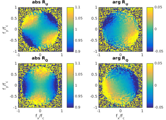
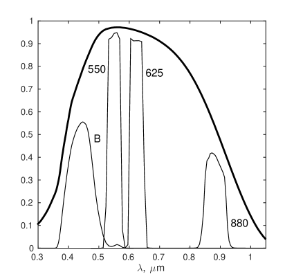
Figure 1: Left panel: the measurement of $\mathcal{R}$ for Betelgeuse on 2019-12-11 in band 550 nm. Spatial frequency normalized by cut–off frequency $f_{c}=D/\lambda$ of the system is along the axes. $D$ — aperture diameter. North is up, East is left. Right panel: thin lines are the passbands of the filters employed in this work multiplied by the quantum efficiency of the detector Andor iXon 897 (thick line).

For the stars without polarized circumstellar structures $\widetilde{Q}(\boldsymbol{f})=0$ and $\widetilde{U}(\boldsymbol{f})=0$ $\forall\boldsymbol{f}$, therefore $\mathcal{R}=1$ is expected. The example of $\mathcal{R}$ measurement for Betelgeuse is given in Fig. 1. One can tell that $\mathcal{R}$ significantly deviates from 1, which gives evidence for the existence of a polarized nebula. The butterfly pattern in $\mathcal{R}$ is very typical for a reflection nebula (Norris et al., 2012, Haubois et al., 2019). The phase of $\mathcal{R}$ significantly deviates from zero, hinting the asymmetry of polarized flux distribution.

Safonov et al. (2019a) describe how the $\mathcal{R}$ value can be used for the reconstruction of polarized intensity distribution of the envelope, given that both its amplitude and phase is known. This reconstruction implies that the object is dominated by a point–like and unpolarized star. At the same time, Betelgeuse has an angular size which we cannot neglect. Moreover, according to Montarges et al (2020), the star lacks the point symmetry. In Appendix B we demonstrate that both factors do not affect the reconstructed images much.

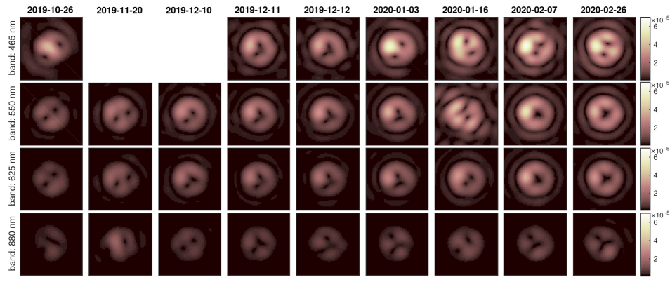
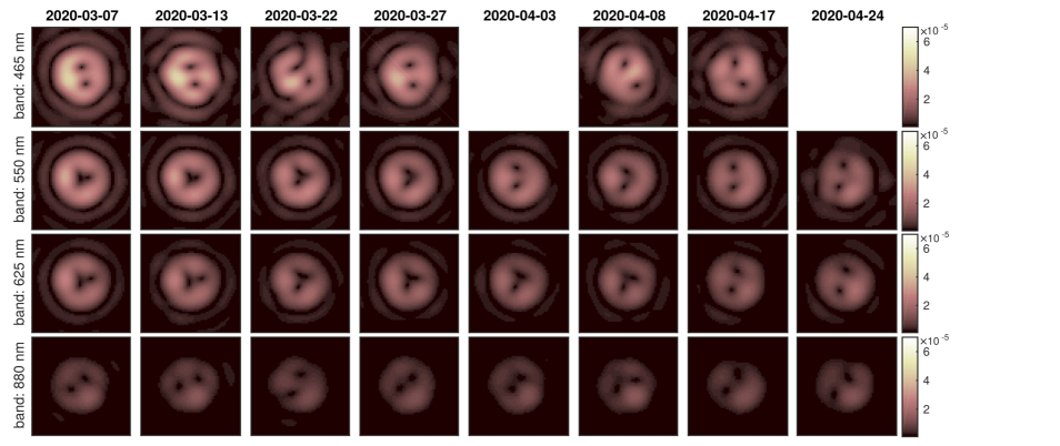
Figure 2: The images of circumstellar envelope of Betelgeuse in polarized light, reconstructed using the method described by Safonov et al. (2019a). Some comments are also given in Appendix B of this paper. The pixel size is 5 mas, which is 4 times smaller than the initial angular scale of the camera. The brightness is proportional to polarized flux in the pixel relative to net unpolarized flux of the object. The size of displayed region is 0.3$\times$0.3^′′, North is up, East is left. Rows correspond to bands, columns — to dates. On some dates observations in the $B$ band were not conducted.

The reconstructed images are presented in Fig. 2 for all the obtained observations. The images for all the filters were convolved with diffraction–limited point spread function, corresponding to $\lambda=880$, thus allowing for the direct comparison of spatial scales.

The azimuthal pattern of polarization is present in all the images — the polarization plane is oriented normally to local direction to the star center. Thus, for clarity, the polarization plane is not plotted. The images for three consecutive dates 2019-12-10, 11, 12 provide a measure of the repeatability of the results. The measurement in the 550 filter made on 2019-01-15 has poor signal–to–noise ratio because atmospheric transparency variations were too large.

Auxiliary spectral observations in visible range were conducted with the Transient Double–beam Spectrograph at the same telescope on 2020-04-06. Due to the extreme brightness of Betelgeuse, we had to defocus its image on the slit in order to obtain 3–5 sec unsaturated exposures. We obtained 4 frames containing spectra. The processing was performed using a specialized pipeline written in python. It consists of the following steps: dark frames subtraction, slit image curvature correction, wavelength calibration using the spectrum of Ne-Kr-Pb light source, spectrum extraction in aperture of fixed width and correction for the response curve.

For the comparison with the spectrum by Levesque and Massey (2020) we averaged our data over 4 measurements, normalized it by continuum and smoothed by running average to match the spectral resolution.

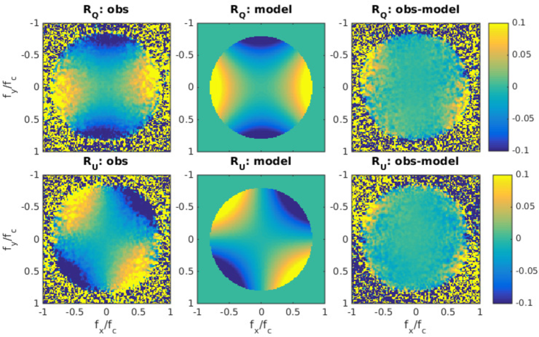
Figure 3: Observational and modelled absolute values of $\mathcal{R}$, and their difference. Upper row — Stokes $Q$, lower — Stokes $U$. Spatial frequency normalized by cut–off frequency is along the axes. The displayed range of signal for all the panels is the same and is given at the right side. The date of observation is 2019-12-11, the band is $550$ nm. Modelling is described in section 3.1.

3 Results

3.1 Envelope brightness

We will start the discussion by considering the total brightness of the resolved envelope. From Fig. 2 one can immediately see that the relative brightness of the envelope is larger for shorter wavelenghts and when the total flux from the object is less (in the minimum). However, quantitative interpretation of images is complicated by smoothing by the point spread function. A direct consideration of $\mathcal{R}$ is more preferable, as long as the latter is an unbiased estimator (Safonov et al., 2019a).

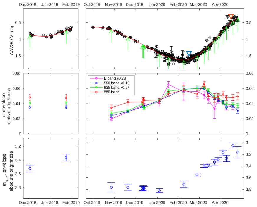
Figure 4: Upper row: black circles are for individual AAVSO $V$ magnitude estimations. Red line is a smoothed light curve. Green arrows denote moments of DSP observations. Blue and orange triangles denote the moments of Levesque and Massey (2020) and our spectral observations, respectively. Middle row: the $\epsilon$ parameter which characterizes the amplitude of butterfly pattern in absolute value of $\mathcal{R}$. It is a proxy of polarized brightness of the envelope relative to the total brightness of the object. Lower row: $m_{\mathrm{env}}$ characterizes the absolute polarized brightness of the envelope with some constant addition.

Under an assumption that the angular size of the scattering envelope is constant, the amplitude of the butterfly pattern in the absolute value of $\mathcal{R}$ will be proportional to the envelope brightness relative to the stellar one. We estimated this amplitude by approximation of $\mathcal{R}$ measurements using the following expressions:

$$|\mathcal{R}_{Q}(\boldsymbol{f})|=1+q-\epsilon\frac{|f|^{2}}{f_{c}^{2}}\cos 2\theta,$$ (2)

$$|\mathcal{R}_{U}(\boldsymbol{f})|=1+u-\epsilon\frac{|f|^{2}}{f_{c}^{2}}\sin 2\theta,$$ (3)

where $|f|$ and $\theta$ are polar coordinates in the Fourier space. $q,u,\epsilon$ are the model parameters, the first two characterize the shift of $\mathcal{R}$ due to non–zero total polarization of the object. $\epsilon$ is the estimate of the amplitude of butterfly pattern. $f_{c}$ is the cut–off frequency of the optical system. In order to compare directly the estimations for all the bands we took the same cut–off frequency $f_{c}=2.84\times 10^{6}$ RAD^-1 for them, which corresponds to $\lambda=880$ nm and an aperture diameter of 2.5 m. We emphasize that $\epsilon$ is only proportional to the relative brightness of the envelope.

The approximation of observational data by the law (2,3) was performed at the frequencies between 0.1$f_{c}$ and 0.4$f_{c}$. Weighting by the inverse squared error of $\mathcal{R}$ was applied as well. The algorithm for estimating the $\mathcal{R}$ error in DSP method is provided by Safonov et al. (2019a). The approximation is illustrated for one particular observation by Fig. 3, very good agreement can be seen.

The dependence of $\epsilon$ on time is given for all the bands in middle row of Fig. 4. It confirms the qualitative conclusions from Fig. 2. The envelope is much brighter at shorter wavelenghts: $\epsilon$ is 3.6 times brighter in $B$ band than at $880$ nm. On the other hand, the relative brightness of the envelope is larger in the minimum.

It is interesting to consider how the absolute brightness of the envelope behaves against the background of stellar variability. For that we computed the following quantity:

$$m_{\mathrm{env}}=-2.5\log_{10}\epsilon+m_{\star},$$ (4)

where $m_{\star}$ is the magnitude of the star (obtained by the interpolation of the AAVSO $V$ magnitude data). This procedure was done only for the 550 band, because its central wavelength is close to that of the $V$ band. $m_{\mathrm{env}}$ corresponds to the polarized absolute brightness of the envelope with some constant addition.

The resulting $m_{\mathrm{env}}$ is presented in the lower row of Fig. 4. During the period from October 2019 to January 2020 this quantity was constant while the star became significantly fainter. This supports the conclusions of Levesque and Massey (2020) that the star decreased its brightness due to a dust cloud localized on the line of sight. The envelope’s brightness stayed constant because the illumination conditions of the envelope surrounding the star did not change.

Since February 2020 the situation had changed, the envelope’s brightness started to rise dramatically. By the end of April 2020 it became 2.1 times brighter than in October 2019 – January 2020 and 1.5 times brighter than a year before.

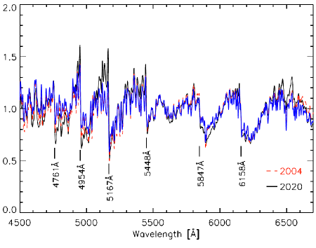
Figure 5: Part of the Betelgeuse spectrum (Fig. 2 from (Levesque and Massey, 2020)). Our spectrum secured on 6th April 2020 is overplotted as blue line.

At the same time the spectrum, which we obtained on April, 6th 2020, almost coincides with the spectra from 2004 and 2020 presented by (Levesque and Massey, 2020), see Fig. 5. The change in the temperature of the photosphere during the whole minimum was not significant and cannot explain the variability of the star and its envelope, see detailed discussion in (Levesque and Massey, 2020).

3.2 Morphology of the envelope

From Fig.2 it can be seen that the scattering envelope significantly deviates from point symmetry. The relative variation of polarized flux at different position angles is around $2-4$. The envelope morphology changes with wavelength and time. The southern part of the envelope appears fainter in the first half of the minimum — the fact which was reported by Montarges et al (2020). Since the mid February 2020 southern part had been brightening and by the end of April it dominated the envelope, especially in 625 and 880 nm bands. One can also note a North-Eastern feature which emerged in November 2019, reached maximum brightness in the mid February and almost disappeared in April 2020.

In order to make the changes in morphology more visible we compiled an animation from the images at 550 nm, which can be found via link. In that animation the images were interpolated pixel–wise on a equidistant temporal grid. Besides, the value in each pixel was multiplied by $2.512^{-m_{V}}$, where $m_{V}$ is an AAVSO magnitude interpolated on the moment of observation. Therefore in the animation an absolute polarized brightness is presented. This is in contrast with Fig.2 where we give polarized brightness relative to the star. The absolute polarized brightness allows one to see once more that before the bottom of the minimum of the star the brightness of the envelope was constant, however it started to rise after this moment.

These structures are visible very clearly at wavelenghts of 465, 550, 625 nm. At 880 nm they are less contrast. However, observations taken in the Nasmyth focus using this band can be distorted by the effects of instrumental polarization. Nevertheless, net polarized brightness of the envelope, which was discussed in previous subsection, is estimated quite reliably. The images restored using observations in the Cassegrain focus (11th and 12th December 2019) are accurate in all the bands.

The features of Betelgeuse’s envelope can be induced by inhomogenuities of the density at the base of dusty wind or by inhomogenuities of illumination of this wind by the photosphere. Both effects are likely to originate from large convective cells on the stellar surface. Similar features of Betelgeuse’s envelope were detected at distances of $1-3R_{\star}$ from the photosphere before by a number Haubois et al. (2019), Kervella et al. (2016), O’Gorman et al. (2017).

4 Conclusion

We present observations of the innermost part of Betelgeuse’s envelope found previously at VLT/NaCO by (Haubois et al., 2019) and at VLT/SPHERE by (Haubois et al., 2019). The envelope is located at $\approx 1R_{\star}$ above the photosphere, it is likely to be the base of dusty wind. The envelope was found to be highly inhomogeneous. Our observations on 17 dates spread over a half the year allowed us to trace the changes of the envelope morphology. For consecutive epochs the observations are highly correlated. A typical timescale of envelope features variability amounts to 2–3 months.

Our observations cover the period of a deep minimum of Betelgeuse’s brightness from October 2019 to April 2020. During this minimum the star became fainter by $1^{m}$ over the period of 3.5 months. Spectral observations by Levesque and Massey (2020) demonstrate that the dimming can be explained by an increase in the amount of absorbing dust in the stellar atmosphere, rather than a decrease in the temperature of the photosphere. According to our data, the total polarized brightness of the envelope was constant during the phase of fainting. This suggests that the increase in circumstellar absorption was significant only for the directions close to the line of sight, while the illumination of the envelope in other directions did not change.

The rise of Betelgeuse’s brightness was approximately two times faster than the fall. Our spectral observations on 2020-04-06 show that the brightening was not related to the change in photosphere temperature either. During the recovery from the minimum the behaviour of the envelope changed dramatically: its polarized brightness started to rise and by 2020-04-24 it was 2.1 times brighter than at the star’s minimum. It is noteworthy that, within 2 months before the minimum, the southern half of the envelope was much darker than the northern (see also (Montarges et al, 2020)). During the recovery from the minimum, the situation changed to the opposite: the southern half dominated the envelope.

The rise of the envelope brightness could be caused by a reduced self–absorption of scattered radiation in it. At the beginning of the minimum the cloud was closer to the star, self–absorption was larger. Then the cloud moved away from the star and its optical depth decreased, as a result, it scattered more light. It is likely that the total amount of scattering material in the envelope increased after the minimum.

The deep minimum of Betelgeuse provides an opportunity to follow the dynamics of dusty clouds in the atmosphere of red supergiant star. In order to construct a quantitative model of this process it is necessary to employ not only scattered light observations similar to ours and that of Montarges et al (2020), but IR observations of thermal radiation of newly formed dust as well. If the star really faded due to the formation of a dust cloud, then a decrease in its brightness should be caused not only by scattering, but also by absorption by the dust. Since the dust particles, absorbing the stellar radiation, heat up, we could expect an increase in the level of IR radiation.

Photometric or spectral data for Betelgeuse in near–IR and mid–IR for the moments before the minimum and close to the bottom of the minimum could made it possible to detect an increase of IR radiation associated with the dimming and confirm the model of dusty cloud formation. Besides, it would allow us to estimate the optical depth and total mass of the condensed dust. If we had at our disposal IR photometric or spectral data in addition to available resolved scattered light observations in visual range, we would be able to trace the evolution of the dusty cloud from the moment of its origin.

From methodological point of view our work demonstrates that a relatively simple instrument mounted at a large telescope could take advantage of the mediocre atmospheric conditions, twilight time or even daytime to study envelopes of evolved stars at spatial scales comparable to 1 stellar radius. Such observations of multiple objects being conducted on a regular basis would be useful for constraining the models of stellar winds similar to (Freytag et al., 2017).

Appendix A Observational log

Observations of Betelgeuse are listed in Table 1. We conducted them preferentially in bad conditions in terms of atmospheric turbulence and transparency. Observations in March–April 2020 were conducted mostly during evening twilight or just before the sunset. Because of that there is no concurrent seeing monitor measurements.

Table 1: Betelgeuse observations circumstances. Columns: 1. focal station: C — Cassegrain, N — Nasmyth; 2. Universal time; 3. Photometric band; 4. Number of accumulated frames; 5. Zenith distance; 6. Sun altitude; 7. Seeing according to automatic seeing monitor (Kornilov et al., 2014).

foc. UT band $N_{\mathrm{fr}}$ $z,^{\circ}$ $h_{\odot},^{\circ}$ $\beta,^{\prime\prime}$ N 18-12-02 23:45 550 3007 41 -49 0.97 N 18-12-02 23:48 625 3002 41 -49 0.95 N 18-12-02 23:52 880 3002 42 -48 0.99 N 19-01-23 20:21 550 3012 41 -63 1.15 N 19-01-23 20:25 625 3011 42 -63 1.18 N 19-01-23 20:28 880 3005 42 -63 0.56 N 19-10-26 22:52 B 6002 44 -50 0.68 N 19-10-26 22:41 550 3002 45 -51 0.83 N 19-10-26 22:44 625 3005 45 -51 0.82 N 19-10-26 22:48 880 3870 44 -50 0.73 N 19-11-20 00:42 B 6003 41 -37 1.20 N 19-11-20 00:33 550 3002 41 -39 1.30 N 19-11-20 00:36 625 3004 41 -38 1.35 N 19-11-20 00:38 880 3009 41 -38 1.23 N 19-12-10 22:28 550 3509 37 -63 1.06 N 19-12-10 22:22 625 3504 37 -63 0.98 N 19-12-10 22:25 880 3507 37 -63 1.40 C 19-12-11 21:38 B 6003 36 -68 0.93 C 19-12-11 21:27 550 3005 36 -69 0.95 C 19-12-11 21:30 625 3002 36 -68 0.91 C 19-12-11 21:33 880 3014 36 -68 0.97 C 19-12-12 20:58 B 6016 37 -69 1.15 C 19-12-12 20:45 550 3008 38 -69 1.02 C 19-12-12 20:48 625 3006 38 -69 1.02 C 19-12-12 20:51 880 3002 38 -69 0.96 N 20-01-03 18:40 B 6010 42 -52 1.14 N 20-01-03 18:31 550 3011 43 -51 1.11 N 20-01-03 18:33 625 3006 42 -51 1.13 N 20-01-03 18:36 880 3003 42 -52 1.13 N 20-01-16 22:35 B 6010 56 -62 1.37 N 20-01-16 22:26 550 3005 54 -63 1.41 N 20-01-16 22:29 625 3011 55 -63 1.35 N 20-01-16 22:32 880 3002 55 -63 — N 20-02-07 16:56 B 6006 39 -27 1.54 N 20-02-07 16:46 550 3011 39 -26 1.15 N 20-02-07 16:49 625 3002 39 -26 1.40 N 20-02-07 16:52 880 3004 39 -27 1.60

foc. UT band $N_{\mathrm{fr}}$ $z,^{\circ}$ $h_{\odot},^{\circ}$ $\beta,^{\prime\prime}$ N 20-02-26 15:57 B 6008 38 -12 1.50 N 20-02-26 15:46 550 3005 38 -11 — N 20-02-26 15:50 625 3012 38 -11 1.54 N 20-02-26 15:53 880 3004 38 -12 1.39 N 20-03-07 17:18 B 6002 40 -25 1.47 N 20-03-07 17:08 550 3002 39 -23 — N 20-03-07 17:11 625 3002 39 -23 1.04 N 20-03-07 17:14 880 3006 40 -24 1.52 N 20-03-13 16:44 B 6003 39 -17 0.96 N 20-03-13 16:35 550 3007 38 -16 1.14 N 20-03-13 16:37 625 3012 39 -16 1.00 N 20-03-13 16:40 880 3004 39 -17 1.00 N 20-03-22 16:45 B 6004 43 -15 — N 20-03-22 16:36 550 3008 42 -14 — N 20-03-22 16:39 625 3008 42 -14 — N 20-03-22 16:42 880 3011 42 -15 — N 20-03-27 15:56 B 6010 40 -6 — N 20-03-27 15:46 550 3002 39 -4 — N 20-03-27 15:49 625 3002 39 -4 — N 20-03-27 15:52 880 3010 39 -5 — N 20-04-03 15:16 550 3010 39 +3 — N 20-04-03 15:19 625 3007 39 +3 — N 20-04-03 15:22 880 3002 39 +2 — N 20-04-08 16:43 B 6003 52 -11 — N 20-04-08 14:21 550 3002 37 +14 — N 20-04-08 14:23 625 3004 37 +14 — N 20-04-08 14:26 880 3006 37 +13 — N 20-04-17 16:00 B 6002 50 -2 — N 20-04-17 15:50 550 3007 49 -0 — N 20-04-17 15:53 625 3002 49 -1 — N 20-04-17 15:56 880 3003 50 -1 — N 20-04-24 15:43 550 3003 52 +3 — N 20-04-24 15:41 625 3003 52 +3 — N 20-04-24 15:35 880 3004 51 +4 —

Appendix B The effect of finite angular size of the star on the image reconstruction

Let us decompose some object into a sum of unpolarized point–like source and polarized extended envelope. The Fourier transforms of Stokes parameters distributions for his object will be (in this appendix the dependence on spatial frequency is omitted):

$$\widetilde{I}=\widetilde{I}_{\star}+\widetilde{I}_{\mathrm{env}},\,\,\,\widetilde{Q}=\widetilde{Q}_{\mathrm{env}},\,\,\,\widetilde{U}=\widetilde{U}_{\mathrm{env}}.$$ (5)

Unpolarized source visibility does not deviate significantly from unity in the probed frequency domain: $\widetilde{I}_{\star}-1\ll 1$. Also it is reasonable to assume that the fraction of polarized radiation is small: $\widetilde{Q}_{\mathrm{env}}\ll\widetilde{I}_{\star}$ and $\widetilde{U}_{\mathrm{env}}\ll\widetilde{I}_{\star}$.

Now we construct the following expressions:

$$S_{Q}=\frac{1-\mathcal{R}_{Q}}{1+\mathcal{R}_{Q}},\,\,\,S_{U}=\frac{1-\mathcal{R}_{U}}{1+\mathcal{R}_{U}}.$$ (6)

Substituting here the definitions (1) and (5) we get:

$$S_{Q}=\frac{\widetilde{Q}_{\mathrm{env}}}{\widetilde{I}_{\star}+\widetilde{I}_{\mathrm{env}}},\,\,\,S_{U}=\frac{\widetilde{U}_{\mathrm{env}}}{\widetilde{U}_{\star}+\widetilde{U}_{\mathrm{env}}}$$ (7)

Taking into account that the denominator in these expressions is close to unity, it is possible to estimate Fourier transforms of Stokes distribution $Q$ and $U$ and then estimate the image of the envelope in polarized light by taking inverse Fourier transforms.

According to Michelson and Pease (1921) the angular diameter of Betelgeuse is 47 mas in visible, which is already comparable with diffraction limited resolution of our instrument: $\lambda/D\approx 50$ mas. The image reconstructed under assumption that $\widetilde{I}_{\star}$ corresponds to a uniform disk with a diameter of 47 mas is presented in Fig. 6.

The same figure contains images reconstructed for the case of elliptical stellar image compressed 2 times along $x$ and $y$ axes. This situation models the appearance of photosphere from (Montarges et al, 2020). As one can see, in all the cases taking into account the finite angular size of the star does not affect much the resulting image. Therefore in this work we assume that $\widetilde{I}_{\star}=1$.

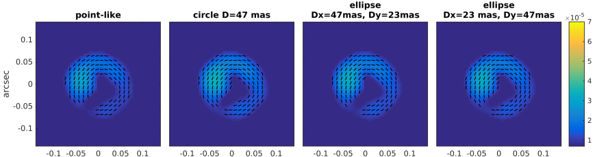
Figure 6: The image of circumstellar envelope of Betelgeuse in polarized light reconstructed by the method described in Appendix B (date 2019-12-11, band 550 nm). From left to right, the source of unpolarized radiation is: 1) point–like 2) uniform disk with diameter of 47 mas 3) uniform ellipse with size of 47 mas along $x$ axis and 23 mas along $y$ axis 4) the same ellipse, but rotated by $90^{\circ}$.

References

- Clarke (2010) D. Clarke. Stellar Polarimetry. 2010.
- Cotton et al. (2020) D. V. Cotton, J. Bailey, A. D. Horta, B. R. M. Norris, and J. R. Lomax. Multi-band aperture polarimetry of betelgeuse during the 2019–20 dimming. Research Notes of the AAS, 4(3):39, mar 2020. doi: 10.3847/2515-5172/ab7f2f. URL https://doi.org/10.3847%2F2515-5172%2Fab7f2f.
- Fedotyeva et al. (2020) A. A. Fedotyeva, A. M. Tatarnikov, B. S. Safonov, V. I. Shenavrin, and G. Komissarova. A Model of the Dust Envelope of the Carbon Mira V CrB from Photometry, Infrared Spectroscopy, and Speckle Polarimetry. Astronomy Letters, 46(1):41–60, Jan. 2020. doi: 10.1134/S1063773720010016.
- Freytag et al. (2017) B. Freytag, S. Liljegren, and S. Höfner. Global 3D radiation-hydrodynamics models of AGB stars. Effects of convection and radial pulsations on atmospheric structures. Astronomy and Astrophysics, 600:A137, Apr. 2017. doi: 10.1051/0004-6361/201629594.
- Guinan et al. (2020) E. Guinan, R. Wasatonic, T. Calderwood, and D. Carona. The Fall and Rise in Brightness of Betelgeuse. The Astronomer’s Telegram, 13512:1, Feb. 2020.
- Haubois et al. (2019) X. Haubois, B. Norris, P. G. Tuthill, C. Pinte, P. Kervella, J. H. Girard, N. M. Kostogryz, S. V. Berdyugina, G. Perrin, S. Lacour, A. Chiavassa, and S. T. Ridgway. The inner dust shell of Betelgeuse detected by polarimetric aperture-masking interferometry. Astronomy and Astrophysics, 628:A101, Aug. 2019. doi: 10.1051/0004-6361/201833258.
- Kervella et al. (2016) P. Kervella, E. Lagadec, M. Montargès, S. T. Ridgway, A. Chiavassa, X. Haubois, H. M. Schmid, M. Langlois, A. Gallenne, and G. Perrin. The close circumstellar environment of Betelgeuse. III. SPHERE/ZIMPOL imaging polarimetry in the visible. Astronomy and Astrophysics, 585:A28, Jan. 2016. doi: 10.1051/0004-6361/201527134.
- Kornilov et al. (2014) V. Kornilov, B. Safonov, M. Kornilov, N. Shatsky, O. Voziakova, S. Potanin, I. Gorbunov, V. Senik, and D. Cheryasov. Study on Atmospheric Optical Turbulence above Mount Shatdzhatmaz in 2007-2013. Publications of the ASP, 126:482–495, May 2014. doi: 10.1086/676648.
- Levesque and Massey (2020) E. M. Levesque and P. Massey. Betelgeuse Just Is Not That Cool: Effective Temperature Alone Cannot Explain the Recent Dimming of Betelgeuse. Astrophysical Journal, Letters, 891(2):L37, Mar. 2020. doi: 10.3847/2041-8213/ab7935.
- Michelson and Pease (1921) A. A. Michelson and F. G. Pease. Measurement of the Diameter of Orionis with the Interferometer. Astrophysical Journal, 53:249–259, May 1921. doi: 10.1086/142603.
- Montarges et al (2020) M. Montarges et al. ESO Telescope Sees Surface of Dim Betelgeuse. ESO press release, Feb. 2020.
- Natta and Panagia (1984) A. Natta and N. Panagia. Extinction in inhomogeneous clouds. Astrophysical Journal, 287:228–237, Dec. 1984. doi: 10.1086/162681.
- Norris et al. (2012) B. R. M. Norris, P. G. Tuthill, M. J. Ireland, S. Lacour, A. A. Zijlstra, F. Lykou, T. M. Evans, P. Stewart, and T. R. Bedding. A close halo of large transparent grains around extreme red giant stars. Nature, 484:220–222, Apr. 2012. doi: 10.1038/nature10935.
- O’Gorman et al. (2017) E. O’Gorman, P. Kervella, G. M. Harper, A. M. S. Richards, L. Decin, M. Montargès, and I. McDonald. The inhomogeneous submillimeter atmosphere of Betelgeuse. Astronomy and Astrophysics, 602:L10, June 2017. doi: 10.1051/0004-6361/201731171.
- Safonov et al. (2019a) B. Safonov, P. Lysenko, M. Goliguzova, and D. Cheryasov. Differential speckle polarimetry at Cassegrain and Nasmyth foci. Monthly Notices of the RAS, 484:5129–5141, Apr. 2019a. doi: 10.1093/mnras/stz288.
- Safonov et al. (2017) B. S. Safonov, P. A. Lysenko, and A. V. Dodin. The speckle polarimeter of the 2.5-m telescope: Design and calibration. Astronomy Letters, 43(5):344–364, May 2017. doi: 10.1134/S1063773717050036.
- Safonov et al. (2019b) B. S. Safonov, A. V. Dodin, S. A. Lamzin, and A. S. Rastorguev. The Circumstellar Envelope of the Semiregular Variable Star V CVn. Astronomy Letters, 45(7):453–461, July 2019b. doi: 10.1134/S1063773719070065.