A Self-Training Method for Machine Reading Comprehension with
Soft Evidence Extraction

Abstract

Neural models have achieved great success on machine reading comprehension (MRC), many of which typically consist of two components: an evidence extractor and an answer predictor. The former seeks the most relevant information from a reference text, while the latter is to locate or generate answers from the extracted evidence. Despite the importance of evidence labels for training the evidence extractor, they are not cheaply accessible, particularly in many non-extractive MRC tasks such as YES/NO question answering and multi-choice MRC.

To address this problem, we present a Self-Training method (STM), which supervises the evidence extractor with auto-generated evidence labels in an iterative process. At each iteration, a base MRC model is trained with golden answers and noisy evidence labels. The trained model will predict pseudo evidence labels as extra supervision in the next iteration. We evaluate STM on seven datasets over three MRC tasks. Experimental results demonstrate the improvement on existing MRC models, and we also analyze how and why such a self-training method works in MRC. The source code can be obtained from https://github.com/SparkJiao/Self-Training-MRC

1 Introduction

Machine reading comprehension (MRC) has received increasing attention recently, which can be roughly divided into two categories: extractive and non-extractive MRC. Extractive MRC requires a model to extract an answer span to a question from reference documents, such as the tasks in SQuAD (Rajpurkar et al., 2016) and CoQA (Reddy et al., 2019). In contrast, non-extractive MRC infers answers based on some evidence in reference documents, including Yes/No question answering (Clark et al., 2019), multiple-choice MRC (Lai et al., 2017; Khashabi et al., 2018; Sun et al., 2019), and open domain question answering (Dhingra et al., 2017b). As shown in Table 1, evidence plays a vital role in MRC (Zhou et al., 2019; Ding et al., 2019; Min et al., 2018), and the coarse-to-fine paradigm has been widely adopted in multiple models (Choi et al., 2017; Li et al., 2018; Wang et al., 2018) where an evidence extractor first seeks the evidence from given documents and then an answer predictor infers the answer based on the evidence. However, it is challenging to learn a good evidence extractor since there lack evidence labels for supervision.

Manually annotating the golden evidence is expensive. Therefore, some recent efforts have been dedicated to improving MRC by leveraging noisy evidence labels when training the evidence extractor. Some works (Lin et al., 2018; Min et al., 2018) generate distant labels using hand-crafted rules and external resources. Some studies (Wang et al., 2018; Choi et al., 2017) adopt reinforcement learning (RL) to decide the labels of evidence, however such RL methods suffer from unstable training. More distant supervision techniques are also used to refine noisy labels, such as deep probability logic (Wang et al., 2019), but they are hard to transfer to other tasks. Nevertheless, improving the evidence extractor remains challenging when golden evidence labels are not available.

Q:	Did a little boy write the note?
D:	…This note is from a little girl. She wants to be your friend. If you want to be her friend, …
A:	No
Q:	Is she carrying something?
D:	…On the step, I find the elderly Chinese lady, small and slight, holding the hand of a little boy. In her other hand, she holds a paper carrier bag. …
A:	Yes

Table 1: Examples of Yes/No question answering. Evidential sentences in bold in reference documents are crucial to answer the questions.

In this paper, we present a general and effective method based on Self-Training (Scudder, 1965) to improve MRC with soft evidence extraction when golden evidence labels are not available. Following the Self-Training paradigm, a base MRC model is iteratively trained. At each iteration, the base model is trained with golden answers, as well as noisy evidence labels obtained at the preceding iteration. Then, the trained model generates noisy evidence labels, which will be used to supervise evidence extraction at the next iteration. The overview of our method is shown in Figure 1. Through this iterative process, evidence is labelled automatically to guide the RC model to find answers, and then a better RC model benefits the evidence labelling process in return. Our method works without any manual efforts or external information, and therefore can be applied to any MRC tasks. Besides, the Self-Training algorithm converges more stably than RL. Two main contributions in this paper are summarized as follows:

1. We propose a self-training method to improve machine reading comprehension by soft evidence labeling. Compared with other existing methods, our method is more effective and general.

2. We verify the generalization and effectiveness of STM on several MRC tasks, including Yes/No question answering (YNQA), multiple-choice machine reading comprehension (MMRC), and open-domain question answering (ODQA). Our method is applicable to different base models, including BERT and DSQA (Lin et al., 2018). Experimental results demonstrate that our proposed method improves base models in three MRC tasks remarkably.

2 Related Work

Early MRC studies focus on modeling semantic matching between a question and a reference document (Seo et al., 2017; Huang et al., 2018; Zhu et al., 2018; Mihaylov and Frank, 2018). In order to mimic the reading mode of human, hierarchical coarse-to-fine methods are proposed (Choi et al., 2017; Li et al., 2018). Such models first read the full text to select relevant text spans, and then infer answers from these relevant spans. Extracting such spans in MRC is drawing more and more attention, though still quite challenging (Wang et al., 2019).

Evidence extraction aims at finding evidential and relevant information for downstream processes in a task, which arguably improves the overall performance of the task. Not surprisingly, evidence extraction is useful and becomes an important component in fact verification (Zhou et al., 2019; Yin and Roth, 2018; Hanselowski et al., 2018; Ma et al., 2019), multiple-choice reading comprehension (Wang et al., 2019; Bax, 2013; Yu et al., 2019), open-domain question answering (Lin et al., 2018; Wang et al., 2018), multi-hop reading comprehension (Nishida et al., 2019; Ding et al., 2019), natural language inference (Wang et al., 2017; Chen et al., 2017), and a wide range of other tasks (Nguyen and Nguyen, 2018; Chen and Bansal, 2018).

In general, evidence extraction in MRC can be classified into four types according to the training method. First, unsupervised methods provide no guidance for evidence extraction (Seo et al., 2017; Huang et al., 2019). Second, supervised methods train evidence extraction with golden evidence labels, which sometimes can be generated automatically in extractive MRC settings (Lin et al., 2018; Yin and Roth, 2018; Hanselowski et al., 2018). Third, weakly supervised methods rely on noisy evidence labels, where the labels can be obtained by heuristic rules (Min et al., 2018). Moreover, some data programming techniques, such as deep probability logic, were proposed to refine noisy labels (Wang et al., 2019). Last, if a weak extractor is obtained via unsupervised or weakly supervised pre-training, reinforcement learning can be utilized to learn a better policy of evidence extraction (Wang et al., 2018; Choi et al., 2017).

For non-extractive MRC tasks, such as YNQA and MMRC, it is cumbersome and inefficient to annotate evidence labels (Ma et al., 2019). Although various methods for evidence extraction have been proposed, training an effective extractor is still a challenging problem when golden evidence labels are unavailable. Weakly supervised methods either suffer from low performance or rely on too many external resources, which makes them difficult to transfer to other tasks. RL methods can indeed train a better extractor without evidence labels. However, they are much more complicated and unstable to train, and highly dependent on model pretraining.

Our method is based on Self-Training, a widely used semi-supervised method. Most related studies follow the framework of traditional Self-Training (Scudder, 1965) and Co-Training (Blum and Mitchell, 1998), and focus on designing better policies for selecting confident samples. CoTrade (Zhang and Zhou, 2011) evaluates the confidence of whether a sample has been correctly labeled via a statistic-based data editing technique (Zighed et al., 2002). Self-paced Co-Training (Ma et al., 2017) adjusts labeled data dynamically according to the consistency between the two models trained on different views. A reinforcement learning based method (Wu et al., 2018) designs an additional Q-agent as a sample selector.

3 Methods

3.1 Task Definition and Model Overview

The task of machine reading comprehension can be formalized as follows: given a reference document composed of a number of sentences $D=\{S_{1},S_{2},\cdots,S_{m}\}$ and a question $Q$, the model should extract or generate an answer $\hat{A}$ to this question conditioned on the document, formally as

$$\hat{A}=\operatorname*{argmax}_{A^{\prime}}P(A^{\prime}|Q,D).$$

The process can be decomposed into two components, i.e., an evidence extractor and an answer predictor. The golden answer $A$ is given for training the entire model, including the evidence extractor and the answer predictor. Denote $E_{i}$ as a binary evidence label $\{0,1\}$ for the $i$-th sentence $S_{i}$, where $0/1$ corresponds to the non-evidence/evidence sentence, respectively. An auxiliary loss on the evidence labels can help the training of the evidence extractor.

The overview of our method is shown in Figure 1, which is an iterative process. During training, two data pools are maintained and denoted as $U$ (unlabeled data) and $L$ (labeled data). In addition to golden answers, examples in $L$ are annotated with pseudo evidence labels. In contrast, there are only golden answers provided in $U$. At each iteration, the base model is trained on both data pools (two training arrows). After training, the model makes evidence predictions on unlabeled instances (the labeling arrow), and then $Selector$ chooses the most confident instances from $U$ to provide noisy evidence labels. In particular, the instances with newly generated evidence labels are moved from $U$ to $L$ (the moving arrow), which are used to supervise evidence extraction in the next iteration. This process will iterate several times.

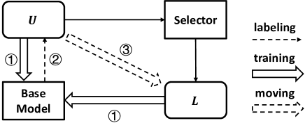
Figure 1: Overview of Self-Training MRC (STM). The base model is trained on both $L$ and $U$. After training, the base model is used to generate evidence labels for the data from $U$, and then $Selector$ chooses the most confident samples, which will be used to supervise the evidence extractor at the next iteration. The selected data is moved from $U$ to $L$ at each iteration.

3.2 Base Model

As shown in Figure 2, the overall structure of a base model consists of an encoder layer, an evidence extractor, and an answer predictor.

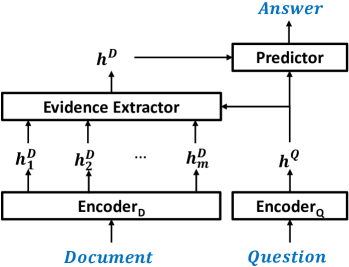
Figure 2: Overall structure of a base model that consists of an encoder layer, an evidence extractor, and an answer predictor. The encoders will obtain $\boldsymbol{h}^{Q}$ for the question, and $\boldsymbol{h}_{i}^{D}$ for each sentence in a document. The summary vector $\boldsymbol{h}^{D}$ will be used to predict the answer.

The encoder layer takes document $D$ and question $Q$ as input to obtain contextual representation for each word. Denote $\boldsymbol{h_{i,j}^{D}}$ as the representation of the $j$-th word in $S_{i}$, and $\boldsymbol{h_{i}^{Q}}$ as the representation of the $i$-th word in question $Q$. Our framework is agnostic to the architecture of the encoder, and we show improvements on two widely used encoding models, i.e. Transformer (with BERT, Devlin et al., 2019) and LSTM (with DSQA, Lin et al., 2018) in the experiments.

The evidence extractor employs hierarchical attention, including token- and sentence-level attention, to obtain the document representation $\boldsymbol{h^{D}}$.

Token-level attention obtains a sentence vector by self-attention (Vaswani et al., 2017) within the words in a sentence, as follows:

$$\boldsymbol{h^{D}_{i}}=\sum^{|S_{i}|}_{j}\alpha_{i,j}\boldsymbol{h^{D}_{i,j}},\;\alpha_{i,j}\propto\exp(F^{S}(\boldsymbol{h^{Q}},\boldsymbol{h^{D}_{i,j}})),$$

$$\boldsymbol{s_{i}^{D}}=\sum^{|S_{i}|}_{j}\beta_{i,j}\boldsymbol{h^{D}_{i,j}},\;\beta_{i,j}\propto\exp(\boldsymbol{w_{s}h^{D}_{i,j}}+b_{s}),$$

where $\boldsymbol{h^{Q}}$ is the sentence representation of the question. $\alpha_{i,j}$ refers to the importance of word $j$ in sentence $i$, and so on for $\beta_{i,j}$. $\boldsymbol{w_{s}}$ and $\boldsymbol{b_{s}}$ are learnable parameters. The attention function $F^{S}$ follows the bilinear form (Kim et al., 2018).

Sentence-level attention identifies important sentences conditioned on the question in a soft way to get the summary vector ($\boldsymbol{h^{D}}$), as follows:

$$\boldsymbol{h^{D}}=\sum^{m}_{i}\gamma_{i}\boldsymbol{h^{D}_{i}},\;\gamma_{i}\propto\exp(F^{D}(\boldsymbol{h^{Q}},\boldsymbol{s_{i}^{D}})),$$

where $F^{D}$ has the same bilinear form as $F^{S}$ with different parameters. $\gamma_{i}$ refers to the importance of the corresponding sentence.

The answer predictor adopts different structures for different MRC tasks. For Yes/No question answering, we use a simple linear classifier to infer answers. For multiple choice MRC, we use a Multiple Layer Perceptron (MLP) with Softmax to obtain the score of each choice. And for open-domain question answering, one MLP is used to predict the answer start, and another MLP is used to predict the end.

3.3 Loss Function

We adopt two loss functions, one for task-specific loss and the other for evidence loss.

The task-specific loss is defined as the negative log-likelihood (NLL) of predicting golden answers, formally as follows:

$$L_{A}(D,Q,A)=-\log P(\hat{A}=A|D,Q),$$

where $\hat{A}$ denotes the predicted answer and $A$ is the golden answer.

When the evidence label $E$ is provided, we can impose supervision on the evidence extractor. For the most general case, we assume that a variable number of evidence sentences exist in each sample $(Q,A,D)$. Inspired by previous work (Nishida et al., 2019) that used multiple evidences, we calculate the evidence loss step by step. Suppose we will extract $K$ evidence sentences. At the first step, we compute the loss of selecting the most plausible evidence sentence. At the second step, we compute the loss in the remaining sentences, where the previously selected sentence is masked and not counted in computing the loss at the second step. The overall loss is the average of all the step-by-step loss until we select out $K$ evidence sentences. In this manner, we devise a BP-able surrogate loss function for choosing the top $K$ evidence sentences.

Formally, we have

$$L_{E}(D,Q,E)=\frac{1}{K}\sum_{k=1}^{K}H(D,Q,E,M^{k}),$$

where $K$ is the number of evidence sentences, a pre-specified hyperparamter. $M^{k}=\{M_{1}^{k},M_{2}^{k},\cdots,M_{m}^{k}\}$ and each $M_{i}^{k}\in\{0,-\infty\}$ is a sentence mask, where $0$ means sentence $i$ is not selected before step $k$, and $-\infty$ means selected.

At each step, the model will compute an attention distribution over the unselected sentences, as follows:

$$\lambda_{i}^{k}=\frac{\exp(F^{D}(\boldsymbol{h^{Q}},\boldsymbol{s_{i}})+M_{i}^{k})}{\sum_{j}(\exp(F^{D}(\boldsymbol{h^{Q}},\boldsymbol{s_{j}})+M_{j}^{k}))}.$$

As $M_{i}^{k}=-\infty$ for the previously selected sentences, the attention weight on those sentences will be zero, in other words, they are masked out. Then, the step-wise loss can be computed as follows:

$$H(D,Q,E,M^{k})=-\log\max_{i}(\lambda_{i}^{k}*E_{i}),$$

where $\lambda_{i}^{k}$ indicates the attention weight for sentence $i$, and $E_{i}\in\{0,1\}$ is the evidence label for sentence $i$. The sentence with the largest attention weight will be chosen as the $k$-th evidence sentence.

For each sentence $i$, $M_{i}^{1}$ is initialized to be $0$. At each step $k(k>1)$, the mask $M_{i}^{k}$ will be set to $-\infty$ if sentence $i$ is chosen as an evidence sentence at the preceding step $k-1$, and the mask remains unchanged otherwise. Formally, the mask is updated as follows:

$$M_{i}^{k}=\left\{\begin{array}[]{ll}-\infty&{i=\operatorname*{argmax}\limits_{j}(\lambda_{j}^{k-1}E_{j})}\\ M_{i}^{k-1}&otherwise\end{array}\right..$$ (3)

During training, the total loss $L$ is the combination of the task-specific loss and the evidence loss:

$$L=\sum_{(D,Q,A)\in U\cup L} L_{A}(D,Q,A)+$$

$$\eta\sum_{(D,Q,E)\in L} L_{E}(D,Q,E),$$ (4)

where $\eta$ is a factor to balance the two loss terms. $L$ and $U$ denote the two sets in which instances with and without evidence labels, respectively. Note that the evidence label in $L$ is automatically obtained in our self-training method.

3.4 Self-Training MRC (STM)

STM is designed to improve base MRC models via generating pseudo evidence labels for evidence extraction when golden labels are unavailable. STM works in an iterative manner, and each iteration consists of two stages. One is to learn a better base model for answer prediction and evidence labelling. The other is to obtain more precise evidence labels for the next iteration using the updated model.

At each iteration, STM first trains the base model with golden answers and pseudo evidence labels from the preceding iteration using the total loss as defined Equation 3.3. Then the trained model can predict a distribution of pseudo evidence labels for each unlabelled instance $(D,Q,A)$, and decides $\hat{E}$ as

$$\hat{E} =\operatorname*{argmin}_{E^{\prime}}L_{E}(D,Q,E^{\prime}).$$ (5)

Define the confidence of a labelled instance $(D,Q,A,\hat{E})$ as

$$c(D,Q,A,\hat{E})= \exp(-L_{A}(D,Q,A))*$$

$$\exp(-L_{E}(D,Q,\hat{E})).$$

$Selector$ selects the instances with the largest confidence scores whose $L_{A}(D,Q,A)$ and $L_{E}(D,Q,\hat{E})$ are smaller than the prespecified thresholds. These labelled instances will be moved from $U$ to $L$ for the next iteration.

In the first iteration (iteration 0), the initial labeled set $L$ is set to an empty set, thus the base model is supervised only by golden answers. In this case, the evidence extractor is trained in a distant supervised manner.

The procedure of one iteration of STM is illustrated in Algorithm 1. $\delta$ and $\epsilon$ are two thresholds (hyper-parameters). $sort$ operation ranks the candidate samples according to their confidence scores $s$ and returns the top-$n$ samples. $n$ varies different datasets, and details are presented in the appendix.

Algorithm 1 One iteration of STM

1:Training sets $U,L$; Thresholds $\delta$ and $\epsilon$; Number of generated labels $n$; Weight of evidence loss $\eta$;

2:Trained MRC model $M$; Updated training sets $U,L$;

3:Randomly initialize $M$;

4:Train $M$ on $U$ and $L$;

5:Initialize $L^{\prime}=\varnothing$;

6:for each $(D,Q,A)\in U$ do

7:     $l_{A}=L_{A}(D,Q,A)$;

8:     Generate $\hat{E}$ via Equation 5;

9:     $l_{\hat{E}}=L_{E}(D,Q,\hat{E})$;

10:     if $l_{A}\leq\delta,l_{\hat{E}}\leq\epsilon$ then

11:         $s=c(D,Q,A,\hat{E})$;

12:         Add $(D,Q,A,\hat{E},s)$ to $L^{\prime}$;

13:     end if

14:end for

15:$L^{\prime}=sort(L^{\prime},n)$;

16:$L=L\cup L^{\prime},U=U\backslash L^{\prime}$;

17:return $M,U,L$;

3.5 Analysis

To understand why STM can improve evidence extraction and the performance of MRC, we revisit the training process and present a theoretical explanation, as inspired by (Anonymous, 2020).

In Section 3.4, we introduce the simple labeling strategy used in STM. If there is no sample selection, the evidence loss can be formulated as

$$\mathcal{L}_{\theta^{t}}=-\mathbb{E}_{x\sim p(x)}\mathbb{E}_{E\sim p_{\theta^{t-1}}(E|x)}\log p_{\theta^{t}}(E|x),$$

where $x$ represents $(D,Q,A)$, and $\theta^{t}$ is the parameter of the $t$-th iteration. In this case, pseudo evidence labels $E$ are randomly sampled from $p_{\theta^{t-1}}(E|x)$ to guide $p_{\theta^{t}}(E|x)$, and therefore minimizing $\mathcal{L}_{\theta^{t}}$ will lead to $\theta^{t}=\theta^{t-1}$. As a matter of fact, the sample selection strategy in STM is to filter out the low-quality pseudo labels with two distribution mappings, $f$ and $g$. The optimizing target becomes

$$\mathcal{L}^{\prime}_{\theta^{t}}=-\mathbb{E}_{x\sim f(p(x))}\mathbb{E}_{E\sim g(p_{\theta^{t-1}}(E|x))}\log p_{\theta^{t}}(E|x).$$

In STM, $f$ is a filter function with two pre-specified thresholds, $\delta$ and $\epsilon$. $g$ is defined as $\operatorname*{argmax}$ (Equation 5). Compared with random sampling, our strategy tends to prevent $\theta^{t}$ from learning wrong knowledge from $\theta^{t-1}$. And the subsequent training might benefit from implicitly learning the strategy. In general, the strategy of STM imposes naive prior knowledge on the base models via the two distribution mappings, which may partly explain the performance gains.

4 Experiments

Model / Dataset	CoQA	MARCO	BoolQ
BERT-MLP	78.0	70.8	71.6
BERT-HA	78.8	71.3	72.9
BERT-HA+RL	79.3	70.3	70.4
BERT-HA+Rule	78.1	70.4	73.8
BERT-HA+STM	80.5†	72.3‡	75.2†
BERT-HA+Gold	82.0	N/A	N/A

Table 2: Classification accuracy on three Yes/No question answering datasets. N/A means there is no golden evidence label. Significance tests were conducted between BERT-HA+STM and the best baseline of each column (t-test). $\ddagger$ means $p$-value $<0.01$, and $\dagger$ means $p$-value $<0.05$.

Model / Dataset	RACE-M		RACE-H		MultiRC			DREAM
	Dev	Test	Dev	Test	Dev			Dev	Test
	Acc	Acc	Acc	Acc	F1m	F1a	EM0	Acc	Acc
GPT+DPL	64.2	62.4	58.5	60.2	70.5	67.8	13.3	57.3	57.7
BERT-MLP	66.2	65.5	61.6	59.5	71.8	69.1	21.2	63.9	63.2
BERT-HA	67.8	68.2	62.6	60.4	70.1	68.1	19.9	64.2	62.8
BERT-HA+RL	68.5	66.9	62.5	60.0	72.1	69.5	21.1	63.1	63.4
BERT-HA+Rule	66.6	66.4	61.6	59.0	69.5	66.7	17.9	62.5	63.0
BERT-HA+STM	69.3‡	69.2†	64.7‡	62.6‡	74.0‡	70.9‡	22.0†	65.3‡	65.8†
BERT-HA+Gold	N/A	N/A	N/A	N/A	73.7	70.9	27.2	N/A	N/A

Table 3: Results on three multiple-choice reading comprehension datasets. (F1_a: F1 score on all answer-options; F1_m: macro-average F1 score of all questions; EM₀: exact match.) Note that there is no golden evidence label on RACE and DREAM. The results for DPL (deep programming logic) are copied from (Wang et al., 2019). Significance tests were conducted between BERT-HA+STM and the best baseline of each column (t-test). $\ddagger$ means $p$-value $<0.01$, and $\dagger$ means $p$-value $<0.05$.

4.1 Datasets

4.1.1 Yes/No Question Answering (YNQA)

CoQA (Reddy et al., 2019) is a multi-turn conversational question answering dataset where questions may be incomplete and need historical context to get the answers. We extracted the Yes/No questions from CoQA, along with their histories, to form a YNQA dataset.

BoolQ (Clark et al., 2019) consists of Yes/No questions from the Google search engine. Each question is accompanied by a related paragraph. We expanded each short paragraph by concatenating some randomly sampled sentences.

MS MARCO (Nguyen et al., 2016) is a large MRC dataset. Each question is paired with a set of reference documents and the answer may not exist in the documents. We extracted all Yes/No questions, and randomly picked some reference documents containing evidence. To balance the ratio of Yes and No questions, we randomly removed some questions whose answers are Yes.

4.1.2 Multiple-choice MRC

RACE (Lai et al., 2017) consists of about 28,000 passages and 100,000 questions from English exams for middle (RACE-M) and high (RACE-H) schools of China. The average number of sentences per passage in RACE-M and RACE-H is about 16 and 17, respectively.

DREAM (Sun et al., 2019) contains 10,197 multiple-choice questions with 6,444 dialogues, collected from English examinations. In DREAM, 85% of the questions require reasoning with multiple evidential sentences.

MultiRC (Khashabi et al., 2018) is an MMRC dataset where the amount of correct options to each question varies from 1 to 10. Each question in MultiRC is annotated with evidence from its reference document. The average number of annotated evidence sentences for each question is 2.3.

4.1.3 Open-domain QA (ODQA)

Quasar-T (Dhingra et al., 2017b) consists of 43,000 open-domain trivial questions, whose answers were extracted from ClueWeb09. For fair comparison, we retrieved 50 reference sentences from ClueWeb09 for each question the same as DSQA (Lin et al., 2018).

4.2 Baselines

We compared several methods in our experiments, including some powerful base models without evidence supervision and some existing methods (*+Rule/RL/DPL/STM) which improve MRC with noisy evidence labels. Experimental details are shown in the appendix.

YNQA and MMRC: (1) BERT-MLP utilizes a BERT encoder and an MLP answer predictor. The predictor makes classification based on the BERT representation at the position of [CLS]. The parameters of the BERT module were initialized from BERT-base. (2) BERT-HA refers to the base model introduced in Section 3.2, which applies hierarchical attention over words and sentences. (3) Based on BERT-HA, BERT-HA+Rule supervises the evidence extractor with noisy evidence labels, which are derived from hand-crafted rules. We have explored three types of rules based on Jaccard similarity, integer linear programming (ILP) (Boudin et al., 2015), and inverse term frequency (ITF) (Wang et al., 2019), among which ITF performed best in most cases. For simplicity, we merely provided experimental results with the rule of ITF. (4) Based on BERT-HA, BERT-HA+RL trains the evidence extractor via reinforcement learning, similar to (Choi et al., 2017). And (5) another deep programming logic (DPL) method, GPT+DPL (Wang et al., 2019), is complicated and the source code is not provided, thus We directly used the results from the original paper and did not evaluate it on BERT.

ODQA: (1) For each question, DSQA (Lin et al., 2018) aggregates multiple relevant paragraphs from ClueWeb09, and then infers an answer from these paragraphs. (2) GA (Dhingra et al., 2017a) and BiDAF (Seo et al., 2017) perform semantic matching between questions and paragraphs with attention mechanisms. And (3) R³ (Wang et al., 2018) is a reinforcement learning method that explicitly selects the most relevant paragraph to a given question for the subsequent reading comprehension module.

Model	EM	F1
GA (Dhingra et al., 2017a)	26.4	26.4
BiDAF (Seo et al., 2017)	25.9	28.5
R3 (Wang et al., 2018)	35.3	41.7
DSQA (Lin et al., 2018)	40.7	47.6
+distant supervision	41.7	48.7
+STM	41.8†	49.2†

Table 4: Experimental results on the test set of Quasar-T. R³ is a RL-based method. Results of GA, BiDAF and R³ are copied from (Lin et al., 2018). DSQA+STM outperforms the best baseline (DSQA+DS) significantly (t-test, $p$-value $<0.05$, DS=distant supervision).

4.3 Main Results

4.3.1 Yes/No Question Answering

Table 2 shows the results on the three YNQA datasets. We merely reported the classification accuracy on the development sets since the test sets are unavailable.

BERT-HA+STM outperformed all the baselines, which demonstrates the effectiveness of our method. Compared with BERT-MLP, BERT-HA achieved better performance on all the three datasets, indicating that distant supervision on evidence extraction can benefit Yes-No question answering. However, compared with BERT-HA, BERT-HA+RL made no improvement on MARCO and BoolQ, possibly due to the high variance in training. Similarly, BERT-HA+Rule performed worse than BERT-HA on CoQA and MARCO, implying that it is more difficult for the rule-based methods (inverse term frequency) to find correct evidence in these two datasets. In contrast, our method BERT-HA+STM is more general and performed the best on all datasets. BERT-HA+STM achieved comparable performance with BERT-HA+Gold which stands for the upper bound by providing golden evidence labels, indicating that the effectiveness of noisy labels in our method.

4.3.2 Multiple-choice MRC

Table 3 shows the experimental results on the three MMRC datasets. We adopt the metrics from the referred papers. STM improved BERT-HA consistently on RACE-H, MultiRC and DREAM in terms of all the metrics. However, the improvement on RACE-M is limited ($1.0$ gain on the test sets). The reason may be that RACE-M is much simpler than RACE-H, and thus, it is not challenging for the evidence extractor of BERT-HA to find the correct evidence on RACE-M.

4.3.3 Open-domain Question Answering

Table 4 shows the exact match scores and F1 scores on Quasar-T. Distant evidence supervision (DS) indicates whether a passage contains the answer text. Compared with the base models DSQA and DSQA+DS, DSQA+STM achieved better performance in both metrics, which verifies that DSQA can also benefit from Self-Training. Our method is general and can improve both lightweight and heavyweight models, like LSTM-based and BERT-based models, in different tasks.

Model/Dataset	CoQA	MultiRC
	P@1	R@1	R@2	R@3	P@1	P@2	P@3
BERT-HA	20.0	28.2	49.8	62.5	62.3	55.2	46.6
+RL	5.2	10.5	22.3	32.9	24.0	25.3	24.7
+Rule	38.4	32.4	53.6	65.1	71.8	59.6	48.7
+STM (iter 1)	32.7	32.8	57.1	70.1	72.2	63.3	52.5
+STM (iter 2)	37.3	32.9	58.0	71.3	72.7	64.4	53.5
+STM (iter 3)	39.9	31.4	55.3	68.8	69.5	61.6	51.6
BERT-HA+Gold	53.6	33.7	59.5	73.4	74.5	65.9	54.8

Table 5: Evidence extraction evaluation on the development sets of CoQA and MultiRC. P@$k$ / R@$k$ represent precision / recall of the generated evidence labels, respectively for top $k$ predicted evidence sentences.

4.4 Performance of Evidence Extraction

To evaluate the performance of STM on evidence extraction, we validated the evidence labels generated by several methods on the development sets of CoQA and MultiRC. Considering that the evidence of each question in MultiRC is a set of sentences, we adopted $precision@k$ and $recall@k$ as the metrics for MultiRC, which represent the precision and recall of the generated evidence labels, respectively, when $k$ sentences are predicted as evidence. We adopted only $precision@1$ as the metric for CoQA as this dataset provides each question with one golden evidence sentence.

Table 5 shows the performance of five methods for evidence labeling on the CoQA and MultiRC development sets. It can be seen that BERT-HA+STM outperformed the base model BERT-HA by a large margin in terms of all the metrics. As a result, the evidence extractor augmented with STM provided more evidential information for the answer predictor, which may explain the improvements of BERT-HA+STM on the two datasets.

4.5 Analysis on Error Propagation

To examine whether error propagation exists and how severe it is in STM, we visualized the evolution of evidence predictions on the development set of CoQA (Figure 3). From the inside to the outside, the four rings show the statistic results of the evidence predicted by BERT-HA (iteration 0) and BERT-HA+STM (iteration 1, 2, 3). Each ring is composed of all the instances from the development set of CoQA, and each radius corresponds to one sample. If the evidence of an instance is predicted correctly, the corresponding radius is marked in green, otherwise in purple. Two examples are shown in the appendix due to space limit.

Self-correction. As the innermost ring shows, about $80\%$ of the evidence predicted by BERT-HA (iter 0) was incorrect. However, the proportion of wrong instances reduced to $60\%$ after self-training (iter 3). More concretely, $27\%$ of the wrong predictions were gradually corrected with high confidence within three self-training iterations, as exemplified by instance A in Figure 3.

Error propagation. We observed that $4\%$ of the evidence was mistakenly revised by STM, as exemplified by instance B in Figure 3. In such a case, the incorrect predictions are likely to be retained in the next iteration. But almost $50\%$ of such mistakes were finally corrected during the subsequent iterations like instance C. This observation shows that STM can prevent error propagation to avoid catastrophic failure.

Figure 3: Evolution of evidence predictions on the development set of CoQA. From the inside to the outside, the four rings correspond to BERT-HA (iteration 0) and BERT-HA+STM (iteration 1, 2, 3), respectively.

4.6 Improvement Over Stronger Pretrained Models

To evaluate the improvement of STM over stronger pretrained models, we employed RoBERTa-large (Liu et al., 2019) as the encoder in the base model. Table 6 shows the results on CoQA. STM significantly improved the evidence extraction (Evi. Acc) of the base model. However, the improvement on answer prediction (Ans. Acc) is marginal. One reason is that RoBERTa-HA achieved so high performance that there was limited room to improve. Another possible explanation is that evidence information is not important for such stronger models to generate answers. In other words, they may be more adept at exploiting data bias to make answer prediction. In comparison, weaker pretrained models, such as BERT-base, can benefit from evidence information due to their weaker ability to exploit data bias.

Model/Metric	Ans. Acc	Evi. Acc
RoBERTa-HA	92.6	13.8
RoBERTa-HA+STM	92.7	19.3(+40%)

Table 6: Answer prediction accuracy (Ans. Acc) and evidence extraction accuracy (Evi. Acc) on the development set of CoQA.

5 Conclusion and Future Work

We present an iterative self-training method (STM) to improve MRC models with soft evidence extraction, when golden evidence labels are unavailable. In this iterative method, we train the base model with golden answers and pseudo evidence labels. The updated model then generates new pseudo evidence labels, which can be used as additional supervision in the next iteration. Experiments results show that our proposed method consistently improves the base models in seven datasets for three MRC tasks, and that better evidence extraction indeed enhances the final performance of MRC.

As future work, we plan to extend our method to other NLP tasks which rely on evidence finding, such as natural language inference.

Appendix A Case Study

In Section 4.5 of the main paper, we provide a quantitative analysis of the evolution of evidence predictions, and draw two conclusions: (1) STM can help the base model to correct itself; (2) Error propagation will not result in catastrophic failure, though exists.

To help understand these two conclusions, we provide two corresponding cases from the development set of CoQA (Reddy et al., 2019). The original instances are shown in Table 7, and the weight distribution from the sentence-level attention is shown in Figure 4. In case 1, BERT-HA made wrong evidence prediction, while STM revised it subsequently, which shows the ability of self-correction. In case 2, BERT-HA first selected the correct evidence with high confidence. However, in the iteration 1, BERT-HA with STM was distracted by another plausible sentence. Instead of insisting on the incorrect prediction, STM led BERT-HA back to the right way, which shows that error propagation is not catastrophic.

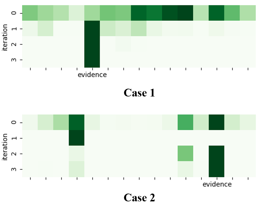
Figure 4: Weight distribution of the two cases from the sentence-level attention.

Appendix B Hyper-Parameters for Self-Training

We implemented BERT-HA with BERT-base from a commonly used library, and directly used the original source code of DSQA (Lin et al., 2018). All the codes and datasets will be released after the review period. The hyper-parameters used in BERT-HA and BERT-HA+STM are shown in Table 8.

(Case 1)

Passage:

…(3)”Why don’t you tackle Indian River, Daylight?” (4)Harper advised, at parting. (5)”There’s whole slathers of creeks and draws draining in up there, and somewhere gold just crying to be found. (6)That’s my hunch. (7)There’s a big strike coming, and Indian River ain’t going to be a million miles away. (8)”And the place is swarming with moose,” Joe Ladue added. (9)”Bob Henderson’s up there somewhere, been there three years now, swearing something big is going to happen, living off’n straight moose and prospecting around like a crazy man.” (10)Daylight decided to go Indian River a flutter, as he expressed it; but Elijah could not be persuaded into accompanying him. Elijah’s soul had been seared by famine, and he was obsessed by fear of repeating the experience. (11)”I jest can’t bear to separate from grub,” he explained. (12)”I know it’s downright foolishness, but I jest can’t help it…”

Question: Are there many bodies of water there?

Answer: No

(Case 2)

Passage:

(1)If you live in the United States, you can’t have a full-time job until you are 16 years old. (2)At 14 or 15, you work part-time after school or on weekends, and during summer vacation you can work 40 hours each week. (3)Does all that mean that if you are younger than 14, you can’t make your own money? (4)Of course not! (5)Kids from 10-13 years of age can make money by doing lots of things. (6)Valerie, 11, told us that she made money by cleaning up other people’s yards. …(11)Kids can learn lots of things from making money. (12)By working to make your own money, you are learning the skills you will need in life. (13)These skills can include things like how to get along with others, how to use technology and how to use your time wisely. (14)Some people think that asking for money is a lot easier than making it; however, if you can make your own money, you don’t have to depend on anyone else…

Question: Can they learn time management?

Answer: No

Table 7: Examples from the development set of CoQA. Evidential sentences in red in reference passages are crucial to answer the questions. Sentences in blue are distracting as Figure 4 shows.

Dataset	RACE-H	RACE-M	DREAM	MultiRC	CoQA	MARCO	BoolQ
$L_{\max}$	380	380	512	512	512	480	512
learning rate	5e-5♣/4e-5♠	5e-5♣/4e-5♠	2e-5	2e-5	2e-5	2e-5	3e-5
epoch	3	3	5	8	3	2♣/3♠	4
$\eta$	0.8	0.8	0.8	0.8	0.8	0.8	0.8
batch size	32	32	32	32	6	8	6
$\epsilon$	0.5	0.5	0.5	0.5	0.6	0.5	0.5
$\delta$	0.9	0.9	0.8	0.8	0.9	0.9	0.7
$n$	40000	10000	3000	2000	1500	1000	500
$K_{\max}$	2	3	4	3	1	1	1

Table 8: Hyper-parameters marked with $\clubsuit$/$\spadesuit$ are used in BERT-HA/BERT-HA+STM, respectively. Other unmarked hyper-parameters are shared by these two models.

References

- Anonymous (2020) Anonymous. 2020. Revisiting self-training for neural sequence generation. ICLR under review.
- Bax (2013) Stephen Bax. 2013. The cognitive processing of candidates during reading tests: Evidence from eye-tracking. Language Testing, 30:441–465.
- Blum and Mitchell (1998) Avrim Blum and Tom M. Mitchell. 1998. Combining labeled and unlabeled data with co-training. In COLT, pages 92–100.
- Boudin et al. (2015) Florian Boudin, Hugo Mougard, and Benoît Favre. 2015. Concept-based summarization using integer linear programming: From concept pruning to multiple optimal solutions. In EMNLP, pages 1914–1918.
- Chen et al. (2017) Qian Chen, Xiaodan Zhu, Zhen-Hua Ling, Si Wei, Hui Jiang, and Diana Inkpen. 2017. Enhanced LSTM for natural language inference. In ACL, pages 1657–1668.
- Chen and Bansal (2018) Yen-Chun Chen and Mohit Bansal. 2018. Fast abstractive summarization with reinforce-selected sentence rewriting. In ACL, pages 675–686.
- Choi et al. (2017) Eunsol Choi, Daniel Hewlett, Jakob Uszkoreit, Illia Polosukhin, Alexandre Lacoste, and Jonathan Berant. 2017. Coarse-to-fine question answering for long documents. In ACL, pages 209–220.
- Clark et al. (2019) Christopher Clark, Kenton Lee, Ming-Wei Chang, Tom Kwiatkowski, Michael Collins, and Kristina Toutanova. 2019. Boolq: Exploring the surprising difficulty of natural yes/no questions. In NAACL, pages 2924–2936.
- Devlin et al. (2019) Jacob Devlin, Ming-Wei Chang, Kenton Lee, and Kristina Toutanova. 2019. BERT: pre-training of deep bidirectional transformers for language understanding. In NAACL, pages 4171–4186.
- Dhingra et al. (2017a) Bhuwan Dhingra, Hanxiao Liu, Zhilin Yang, William W. Cohen, and Ruslan Salakhutdinov. 2017a. Gated-attention readers for text comprehension. In ACL, pages 1832–1846.
- Dhingra et al. (2017b) Bhuwan Dhingra, Kathryn Mazaitis, and William W. Cohen. 2017b. Quasar: Datasets for question answering by search and reading. CoRR, abs/1707.03904.
- Ding et al. (2019) Ming Ding, Chang Zhou, Qibin Chen, Hongxia Yang, and Jie Tang. 2019. Cognitive graph for multi-hop reading comprehension at scale. In ACL, pages 2694–2703.
- Hanselowski et al. (2018) Andreas Hanselowski, Hao Zhang, Zile Li, Daniil Sorokin, Benjamin Schiller, Claudia Schulz, and Iryna Gurevych. 2018. Ukp-athene: Multi-sentence textual entailment for claim verification. CoRR, abs/1809.01479.
- Huang et al. (2019) Hsin-Yuan Huang, Eunsol Choi, and Wen-tau Yih. 2019. Flowqa: Grasping flow in history for conversational machine comprehension. In ICLR.
- Huang et al. (2018) Hsin-Yuan Huang, Chenguang Zhu, Yelong Shen, and Weizhu Chen. 2018. Fusionnet: Fusing via fully-aware attention with application to machine comprehension. In ICLR.
- Khashabi et al. (2018) Daniel Khashabi, Snigdha Chaturvedi, Michael Roth, Shyam Upadhyay, and Dan Roth. 2018. Looking beyond the surface: A challenge set for reading comprehension over multiple sentences. In NAACL, pages 252–262.
- Kim et al. (2018) Jin-Hwa Kim, Jaehyun Jun, and Byoung-Tak Zhang. 2018. Bilinear attention networks. In NIPS, pages 1571–1581.
- Lai et al. (2017) Guokun Lai, Qizhe Xie, Hanxiao Liu, Yiming Yang, and Eduard Hovy. 2017. Race: Large-scale reading comprehension dataset from examinations. In EMNLP, pages 785–794.
- Li et al. (2018) Weikang Li, Wei Li, and Yunfang Wu. 2018. A unified model for document-based question answering based on human-like reading strategy. In AAAI, pages 604–611.
- Lin et al. (2018) Yankai Lin, Haozhe Ji, Zhiyuan Liu, and Maosong Sun. 2018. Denoising distantly supervised open-domain question answering. In ACL, pages 1736–1745.
- Liu et al. (2019) Yinhan Liu, Myle Ott, Naman Goyal, Jingfei Du, Mandar Joshi, Danqi Chen, Omer Levy, Mike Lewis, Luke Zettlemoyer, and Veselin Stoyanov. 2019. Roberta: A robustly optimized BERT pretraining approach. CoRR, abs/1907.11692.
- Ma et al. (2017) Fan Ma, Deyu Meng, Qi Xie, Zina Li, and Xuanyi Dong. 2017. Self-paced co-training. In ICML, pages 2275–2284.
- Ma et al. (2019) Jing Ma, Wei Gao, Shafiq R. Joty, and Kam-Fai Wong. 2019. Sentence-level evidence embedding for claim verification with hierarchical attention networks. In ACL, pages 2561–2571.
- Mihaylov and Frank (2018) Todor Mihaylov and Anette Frank. 2018. Knowledgeable reader: Enhancing cloze-style reading comprehension with external commonsense knowledge. In ACL, pages 821–832.
- Min et al. (2018) Sewon Min, Victor Zhong, Richard Socher, and Caiming Xiong. 2018. Efficient and robust question answering from minimal context over documents. In ACL, pages 1725–1735.
- Nguyen and Nguyen (2018) Minh Nguyen and Thien Nguyen. 2018. Who is killed by police: Introducing supervised attention for hierarchical lstms. In COLING, pages 2277–2287.
- Nguyen et al. (2016) Tri Nguyen, Mir Rosenberg, Xia Song, Jianfeng Gao, Saurabh Tiwary, Rangan Majumder, and Li Deng. 2016. MS MARCO: A human generated machine reading comprehension dataset. In NIPS.
- Nishida et al. (2019) Kosuke Nishida, Kyosuke Nishida, Masaaki Nagata, Atsushi Otsuka, Itsumi Saito, Hisako Asano, and Junji Tomita. 2019. Answering while summarizing: Multi-task learning for multi-hop QA with evidence extraction. In ACL, pages 2335–2345.
- Rajpurkar et al. (2016) Pranav Rajpurkar, Jian Zhang, Konstantin Lopyrev, and Percy Liang. 2016. Squad: 100, 000+ questions for machine comprehension of text. In EMNLP, pages 2383–2392.
- Reddy et al. (2019) Siva Reddy, Danqi Chen, and Christopher D. Manning. 2019. Coqa: A conversational question answering challenge. TACL, 7:249–266.
- Scudder (1965) H. J. Scudder. 1965. Probability of error of some adaptive pattern-recognition machines. IEEE Trans. Information Theory, 11.
- Seo et al. (2017) Min Joon Seo, Aniruddha Kembhavi, Ali Farhadi, and Hannaneh Hajishirzi. 2017. Bidirectional attention flow for machine comprehension. In ICLR.
- Sun et al. (2019) Kai Sun, Dian Yu, Jianshu Chen, Dong Yu, Yejin Choi, and Claire Cardie. 2019. DREAM: A challenge dataset and models for dialogue-based reading comprehension. TACL, 7:217–231.
- Vaswani et al. (2017) Ashish Vaswani, Noam Shazeer, Niki Parmar, Jakob Uszkoreit, Llion Jones, Aidan N. Gomez, Lukasz Kaiser, and Illia Polosukhin. 2017. Attention is all you need. In NIPS, pages 6000–6010.
- Wang et al. (2019) Hai Wang, Dian Yu, Kai Sun, Jianshu Chen, Dong Yu, Dan Roth, and David A. McAllester. 2019. Evidence sentence extraction for machine reading comprehension. CoRR, abs/1902.08852.
- Wang et al. (2018) Shuohang Wang, Mo Yu, Xiaoxiao Guo, Zhiguo Wang, Tim Klinger, Wei Zhang, Shiyu Chang, Gerry Tesauro, Bowen Zhou, and Jing Jiang. 2018. R: Reinforced ranker-reader for open-domain question answering. In AAAI, pages 5981–5988.
- Wang et al. (2017) Zhiguo Wang, Wael Hamza, and Radu Florian. 2017. Bilateral multi-perspective matching for natural language sentences. In IJCAI, pages 4144–4150.
- Wu et al. (2018) Jiawei Wu, Lei Li, and William Yang Wang. 2018. Reinforced co-training. In NAACL, pages 1252–1262.
- Yin and Roth (2018) Wenpeng Yin and Dan Roth. 2018. Twowingos: A two-wing optimization strategy for evidential claim verification. In EMNLP, pages 105–114.
- Yu et al. (2019) Jianxing Yu, Zhengjun Zha, and Jian Yin. 2019. Inferential machine comprehension: Answering questions by recursively deducing the evidence chain from text. In ACL, pages 2241–2251.
- Zhang and Zhou (2011) Min-Ling Zhang and Zhi-Hua Zhou. 2011. Cotrade: Confident co-training with data editing. TSMCB, 41:1612–1626.
- Zhou et al. (2019) Jie Zhou, Xu Han, Cheng Yang, Zhiyuan Liu, Lifeng Wang, Changcheng Li, and Maosong Sun. 2019. GEAR: graph-based evidence aggregating and reasoning for fact verification. In ACL, pages 892–901.
- Zhu et al. (2018) Chenguang Zhu, Michael Zeng, and Xuedong Huang. 2018. Sdnet: Contextualized attention-based deep network for conversational question answering. CoRR, abs/1812.03593.
- Zighed et al. (2002) Djamel A. Zighed, Stéphane Lallich, and Fabrice Muhlenbach. 2002. Separability index in supervised learning. In PKDD, pages 475–487.