Three Mechanisms for Bar Thickening

Abstract

We present simulations of bar-unstable stellar discs in which the bars thicken into box/peanut shapes. Detailed analysis of the evolution of each model revealed three different mechanisms for thickening the bars. The first mechanism is the well-known buckling instability, the second is the vertical excitation of bar orbits by passage through the 2:1 vertical resonance, and the third is a gradually increasing fraction of bar orbits trapped into this resonance. Since bars in many galaxies may have formed and thickened long ago, we have examined the models for fossil evidence in the velocity distribution of stars in the bar, finding a diagnostic to discriminate between a bar that had buckled from the other two mechanisms.

1 Introduction

Many disc galaxies possess bars (e.g. Erwin, 2018). A bar is usually the strongest non-axisymmetric feature in the light distribution (e.g. Díaz-García et al., 2016) and is often, but not always, centered on the photometric and kinematic centre of the galaxy. The material that makes up a bar manifests considerable non-circular streaming motion (Kormendy, 1983; Weiner et al., 2001; Aguerri et al., 2015; Holmes et al., 2015), indicating a strongly non-axisymmetric gravitational field. Many galaxies that are viewed edge-on manifest a boxy or peanut shaped bulge (Shaw, 1987; Lütticke, Dettmar & Pohlen, 2000; Erwin & Debattista, 2017), which is interpreted (Combes & Sanders, 1981; Kuijken & Merrifield, 1995; Bureau & Athanassoula, 2005) to be a bar that has become thicker than the surrounding disc.

The Milky Way possesses a strong bar seen in oblique projection from the Sun’s location (Bland-Hawthorn & Gerhard, 2016). It consists of both a thick (Weiland et al., 1994; Binney, Gerhard & Spergel, 1997) and a thin bar component (Hammersley et al., 2000; Wegg et al., 2015). The thick component has a strong peanut shape seen in star counts (McWilliam & Zoccali, 2010; Wegg & Gerhard, 2013) and infrared photometry (Ness & Lang, 2016). Both gas (Dame, Hartmann & Thaddeus, 2001) and stars (Rangwala et al., 2009; Sanders et al., 2019) in the inner Galaxy show strong non-circular streaming motions dominated by the bar (Fux, 1999; Li et al., 2016; Shen et al., 2010; Portail et al., 2017), and as in external boxy-peanut bulges, the stellar velocity field shows cylindrical rotation (Howard et al., 2009).

Sellwood & Wilkinson (1993) and Binney & Tremaine (2008) have summarized much of the old theoretical work that had led to considerable insight into the structure of bars. For the most part, this body of work considered the bar to be a steadily rotating rigid object, and Sparke & Sellwood (1987) found most of the expected orbit families in the frozen the potential of their 2D $N$-body bar. More recently, Valluri et al. (2016) used orbits from their simulations to demonstrate the relationships between the traditional classification of orbits in bars with those of tri-axial ellipsoids, while Gajda et al. (2016) found that the bar in their simulation was sufficiently steady that they could fit a steadily rotating bar model and apply the more modern apparatus of frequency analysis developed by Laskar (1990). Portail et al. (2015) and Abbott et al. (2017) also studied the 3D shapes of particle orbits in the frozen potentials of their $N$-body bars, focusing in both cases on orbits that supported the peanut shape.

Many authors have reported simulations in which a bar thickened as a result of a buckling instability (e.g. Raha et al., 1991; Debattista et al., 2005; Martinez-Valpuesta et al., 2006; Collier, 2020). Following Combes & Sanders (1981), Combes et al. (1990) suggested that the thickening mechanism was related to a resonance between the frequencies of the periodic motions along and normal to the bar mid-plane. This more gradual mechanism was further developed by Quillen et al. (2014), who elegantly described how the vertical motions of stars could be increased as the resonance swept past them.

In this paper, we study how the structure of a bar changes as it evolves, an objective shared by Petersen et al. (2016, 2019a, 2019b). Their papers concentrated on the halo distortion, the in-plane motion in the bar, and torques, but our principal focus here is on the mechanisms of bar thickening in the evolving potential of the simulated bar (see also Łokas, 2019, who focused on the buckling instability only). We present simulations that illustrate three thickening mechanisms: one in which the bar thickened through a buckling instability, and a second that seems to show that bar orbits were heated vertically by the passage through the 2:1 vertical resonance, as described by Quillen et al. (2014). We were surprised to find a third mechanism of gradual trapping of orbits into the 2:1 resonance that has not previously been identified in simulations, to our knowledge, but had been proposed by Quillen (2002). We found this behaviour in a somewhat slow bar, i.e. one in which corotation was 1.6 times the bar semi-major axis, a larger than usual fraction (e.g. Aguerri et al., 2015).

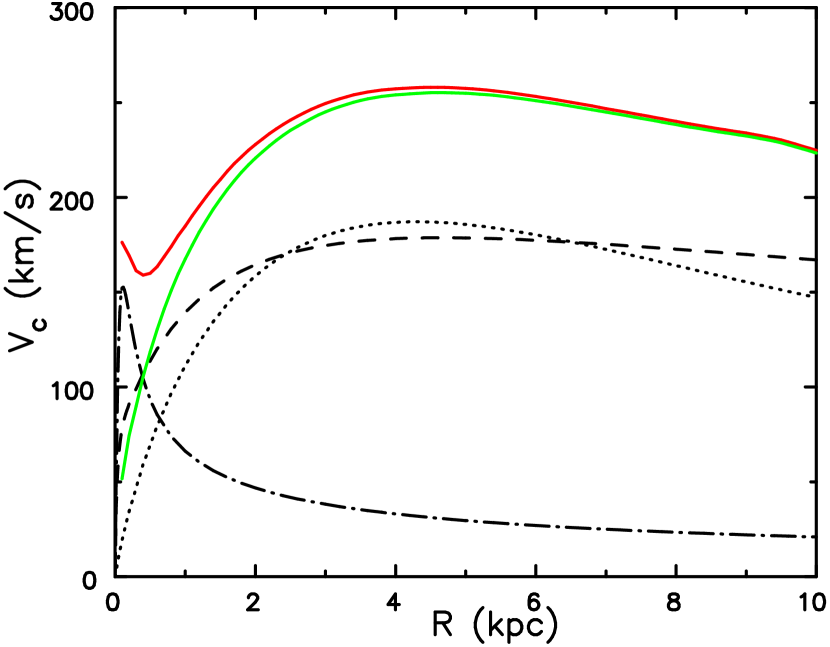
Figure 1: The initial rotation curves of our models with (red) a nuclear star cluster and without (green). These curves are determined from the particles. The other lines indicate the separate contributions of the individual components: the disc (dotted), the nuclear star cluster (dot-dashed), and the Hernquist halo compressed, in this case, by both the disc and the nuclear star cluster (dashed). The scaling from model units to physical units is described in the text.

2 Technique

We use collisionless simulations to study the processes of bar thickening, and start from bar-unstable equilibrium disc models embedded in spherical halos. Our models for the disc and halo were selected for convenience only, with no inention to match any particular galaxy.

2.1 Mass models

We create models of discs and halos, and in some cases add a nuclear mass component, all composed of particles. The disc is an exponential with a Gaussian vertical density profile

$$\rho_{d}(R,z)={M_{d}\over(2\pi)^{3/2}R_{d}^{2}z_{0}}e^{-(R/R_{d}+z^{2}/2z_{0}^{2})}$$ (1)

where $M_{d}$ is the disc mass, $R_{d}$ the scale length, and $z_{0}=0.1R_{d}$. The disc surface density is tapered to zero using a cubic polynomial over the radial range $4.5<R/R_{d}<5.0$.

We use an initially isotropic spherical Hernquist halo (Hernquist, 1990) having the density profile

$$\rho_{h}(r)={M_{h}\over 2\pi}{r_{h}^{4}\over r(r+r_{h})^{3}},$$ (2)

where $M_{h}=10M_{d}$ and $r_{h}=5R_{d}$. We allow for the presence of the additional components (the disc and perhaps a nuclear component) by compressing the halo adiabatically by the method described by Sellwood & McGaugh (2005).

In some models we added a nuclear star cluster modeled as an isotropic Plummer sphere having a mass $M_{d}/40$ and a core radius of $R_{d}/20$.

The disc particles were given equilibrium orbital velocities with an initial radial velocity dispersion, $\sigma_{R}$, so that $Q=1$ (neglecting corrections for disc thickness and gravity softening) at all radii, where

$$Q=\sigma_{R}{\kappa\over 3.36G\Sigma},$$ (3)

$\Sigma(R)$ is the projected surface density, and $\kappa(R)$ is the numerically-estimated epicyclic frequency in the disc mid-plane. The azimuthal dispersion, asymmetric drift, and vertical velocity dispersion are all set by solving the Jeans equations (Binney & Tremaine, 2008).

Although our models were not intended to match the Milky Way, in which the inner halo has a lower density (Portail et al., 2017), we nevertheless scale them to the Milky Way. Choosing $R_{d}=2\;$kpc and a dynamical time $\tau_{\rm dyn}\equiv(R_{d}^{3}/GM_{d})^{1/2}=6.5\;$Myr yields bar sizes that resemble that in the Milky Way, an orbital speed of $\sim 250\;$km s^-1 at a radius of 8 kpc in the disc mid-plane, and a disk scale height $z_{0}=200\;$pc. These choices imply a mass unit, the mass of the disc, $M_{d}\simeq 4.21\times 10^{10}\;$M_⊙, a unit of velocity $R_{d}/\tau_{\rm dyn}\simeq 301\;$km s^-1, and a frequency unit of $\tau_{\rm dyn}^{-1}\simeq 47.7\;$km s^-1 kpc^-1.

The initial rotation curves of our equilibrium models with (red) and without (green) a nuclear star cluster are illustrated in Figure 1.

Table 1: Numerical parameters

Polar grid size	85 $\times$ 128 $\times$ 125
$z$ spacing	$0.02R_{d}=40\;$pc
Active sectoral harmonics	$0\leq m\leq 8$
Grid distance unit ($h_{R}$)	$0.1R_{d}=200\;$pc
Softening length	$0.1R_{d}=200\;$pc
Spherical grid size	500 shells
Outer radius	$60R_{d}=120\;$kpc
Active spherical harmonics	$0\leq l\leq 4$
Number of disc particles	$10^{6}$
Number of halo particles	$10^{6}$
Basic time-step	$0.01[R_{d}^{3}/(GM_{d})]^{1/2}=6.5\times 10^{4}\;$yr
Time step zones	5

2.2 Numerical method

We evolve these models using the hybrid grid option of the GALAXY code, which is fully described in the on-line manual (Sellwood, 2014); the code itself is available for download. The mutual attractions of all particles are computed at every step. To achieve this, we employ a cylindrical polar 3D grid to compute the gravitational field of the disc particles together with a spherical grid for the halo and nuclear star cluster, if present. For efficiency, we use block time steps in a series of spatially-defined, spherical zones, in which particles farther from the centre move on time steps that are successively increased by factors of two for zones more distant from the centre.

Table 1 gives the values of the numerical parameters for simulations lacking a nuclear mass component. We shorten the basic time step by a factor of 4 and include 2 extra time step zones when a nuclear star cluster, represented by $2.5\times 10^{4}$ particles is present. We have verified that our results are insensitive to reasonable changes to these numerical parameters.

3 Results

We computed the evolution of all models to $5.2\;$Gyr, during which time they all formed strong bars. The bars in models with a nuclear mass component tended not to buckle, and instead puffed up gradually over time, whereas those in models that lacked the dense central component did buckle soon after their formation, but also continued to puff up over time. While we have computed many models, we present just three in this section.

Figure 2: Model A: The time evolution of (a) the bar amplitude, (b) the bar length (solid line) and (c) the bar pattern speed. (d) Radial variation of the azimuthally averaged rms thickness of disc particles at intervals of $0.65\;$Gyr from $t=0$ to $t=5.2\;$Gyr. The thickness increases monotonically at most radii.

3.1 A bar that buckled

We first describe model A, which lacked a nuclear mass component. The initial equilibrium disc was globally unstable to the formation of a bar, which had developed by $t\sim 0.7\;$Gyr. The bar later buckled in the usual way at $t\sim 1.5\;$Gyr.

Figure 2 presents the time evolution of (a) the amplitude, (b) semi-major axis $a_{\rm B}$, (c) pattern speed of the bar, and (d) the radial variation of the rms $z$-thickness of the disc particles at intervals of 0.65 Gyr. The bar amplitude is $A_{2}/A_{0}(t)=|\sum_{j}e^{2i\phi_{j}}|/N_{d}$, where $\phi_{j}(t)$ is the azimuth of the $j$-th disc particle at time $t$ and $N_{d}$ is the number of disc particles, which all have equal mass. The bar length (panel b) is the average of the two dotted curves, which were estimated by the methods described in Debattista & Sellwood (2000). The initial semi-major axis is $a_{B}\la 4\;$kpc, but by $t=2.6\;$Gyr it had grown in length to $a_{B}\approx 6\;$kpc. The pattern speed (panel c) decreased rapidly to $t\sim 2\;$Gyr due to friction with the halo, which weakened over time. At late times, the corotation radius $R_{\rm CR}\la 8\;$kpc so that the dimensionless ratio ${\cal R}\equiv R_{\rm CR}/a_{B}\sim 1.3$.

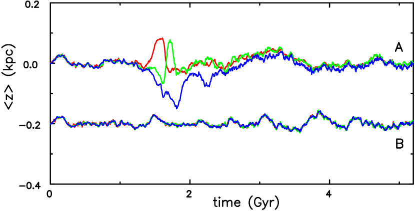
Figure 3: The time evolution of the mean $z$-height of particles in three radial bins of width 400 pc centered on 1 kpc (red), 2.2 kpc (green) and 3.4 kpc (blue) in models A and B. Values for model B have been shifted by $-200$ pc for clarity.

Figure 3 displays the time evolution of the mean $z$-coordinate of the disc particles in three different radial bins for this model and for model B. The curves of different colours, which indicate different radial bins, separate for the period $1.3\la t\la 2.5\;$Gyr indicating that the disc, which is dominated by the bar at these radii, is flexing.

The vertical thickness of the bar (Figure 2d) increased substantially between the third and fourth curves, which are for $t=1.3$ and $t=1.95\;$Gyr respectively; this interval brackets the time of the buckling instability. The bar continued to puff up more gradually until the last time shown ($t=5.2\;$Gyr). The radial range of the thickest part of the bar is $2\la R\la 4\;$kpc, thus the outermost $\sim 1/3$ of its length could be described as a “thin bar”, which had a thickness similar to that of the disc just beyond the bar’s end.

The bar also weakens temporarily at the time of buckling instability (Figure 2a), as has been reported before (e.g. Raha et al., 1991; Martinez-Valpuesta & Shlosman, 2004; Debattista et al., 2005).

Figure 4: Model B: The time evolution of (a) the bar amplitude, (b) the bar length (solid line) and (c) the bar pattern speed. (d) Radial variation of the azimuthally averaged rms thickness of disc particles at intervals of $0.65\;$Gyr from $t=0$ to $t=5.2\;$Gyr. The thickness increases monotonically at most radii.

3.2 A bar that did not buckle

We included the nuclear star cluster described in §2.1 in model B, which also formed a strong bar. Linear stability theory would predict that such a dense central mass should prevent bar formation by inserting an inner Lindbald resonance to block the feedback loop that drives the instability (Toomre, 1981; Binney & Tremaine, 2008), but non-linear orbit trapping (e.g. Sellwood, 1989) generally overwhelms the resonance in most simulations, allowing a bar to form.

Figure 4 shows that the bar took a little longer to develop than in model A, but it was well established by $\sim 2\;$Gyr when it had already begun to thicken. However, it did not appear to buckle at any time, as shown in Figure 3. Values of $\langle z\rangle$ in model B fluctuated over time, but the blue line almost perfectly overlays the red and green lines, indicating that mid-plane moved equally at all three radii, and that the bar was not flexing. This contrasts with the behaviour in model A in the same Figure, in which different radial ranges were displaced in opposite senses for a period.

The initial bar in model B has $a_{B}\simeq 3\;$kpc (Figure 4b), and it grows to $a_{B}\simeq 5.2\;$kpc by the end. Again the bar pattern speed (panel c) slowed rapidly at first and then more gradually. The time variation of the corotation radius, $R_{\rm CR}$, and $a_{\rm B}$ conspired to make their dimensionless ratio ${\cal R}\simeq 1.4$ for most of the evolution.

Panel (d) shows that by $t=1.95\;$Gyr (the fourth curve), the bar had thickened over the range $1\leq R\leq 2\;$kpc, and it continued to thicken as it also grew in length. As for model A, the outer bar ($4\la R\la 5.2\;$kpc) is no thicker than the disc beyond the bar end at later times, while the thickest part of the bar lies between $1\la R\la 3\;$kpc.

Figure 5: Model C: The time evolution of (a) the bar amplitude, (b) the bar length (solid line) and (c) the bar pattern speed. (d) Radial varition of the azimuthally averaged rms thickness of disc particles at intervals of $0.65\;$Gyr from $t=0$ to $t=5.2\;$Gyr. The thickness increases monotonically at most radii.

3.3 A remarkable comparison

It is possible to inhibit the buckling instability by imposing reflection symmetry about the mid-plane at each step of the simulation, as reported by Friedli & Pfenniger (1990). This is easily achieved with a grid-code, such as GALAXY, by replacing the masses assigned to the grid points by the average of the values above and below the mid-plane before determining the gravitational field.

We pursued this strategy in model C, which was identical in every respect to model A except for the imposition of vertical reflection symmetry. As we intended, the buckling instability of the bar was indeed inhibited, but the evolution of the bars differed from those in model A to a surprising extent.

Because the buckling instability was suppressed, the bar amplitude grew monotonically (Fig. 5a), but the final bar amplitude in C was more than 50% greater than in model A (Fig. 2a). The bar semi-axes started at the same value, as expected, although the bar became longer when buckling was supressed (panel b). The increased bar amplitudes and lengths over that in models A created a stronger quadrupole moment that caused stronger friction with the halo, slowing the bar to a greater extent (panel c), and causing the dimensionless ratio to rise to ${\cal R}\ga 1.6$. In fact, the disc component of model C had lost over 30% of its initial angular momentum to the halo by the end of the run, which is twice that lost in model A.

But the most surprising consequence of inhibiting buckling is that the vertical thickness of the bar in C continued to grow throughout the evolution, reaching much greater values (Fig. 5d) than in model A (Fig. 2d); i.e. suppressing buckling resulted much thicker final bar! Furthermore, the bar thickened over almost its entire extent, save for the very centre, and there was little if any outer thin bar.

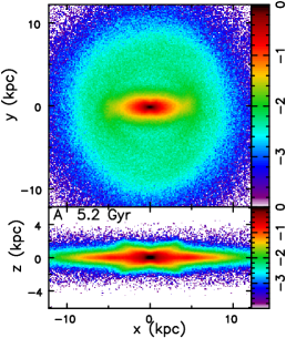
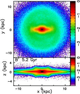
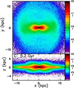
Figure 6: Snapshots of models A (left), B (middle), and C (right) at the final time. The logarithmic colour scale indicates projected density of the disc particles only, normalized to its peak value in each panel. Each model has been rotated so that the bar is horizontal, and the lower panels show the edge-on view.

3.4 Visual comparison

Figure 6 presents snapshots of models A, B, and C at the final time. Note that the shapes of the bars in the pole-on projection are all quite different. The bar in model A is oval and that in model B is more lens-shaped with a near axisymmetric centre. The high density inner bar in model C has a more butterfly shape, while the low-density outer bar is again oval. The vertical thicknesses all differ, as already reported, and it can be seen that the greater thickness of the bar in model C largely stems from a low-density envelope around the high density in the mid-plane.

4 Analysis

It is well known that bars become vertically thicker as a result of the buckling instability (Raha et al., 1991; Sellwood & Merritt, 1994). Combes et al. (1990) argued for an alternative mechanism involving the 2:1 vertical resonance, at which $\Omega_{z}=2\Omega_{x}$; here $\Omega_{z}$ is the vertical freqency and $\Omega_{x}$ is the frequency of oscillation along the bar major axis in the rotating bar frame. Quillen et al. (2014) developed this second idea and found that orbits could be elevated by becoming trapped in the resonance, and argued that the resonance sweeps outwards as the bar evolves, allowing orbits to be later released from the resonance with an increased vertical oscillation amplitude. Quillen et al. (2014) claimed evidence in support of their thickening mechanism from analysis of a few snapshots taken from archival simulations. Here we mount a much more robust test of their proposed mechanism.

The bars in our models evolve continuously in pattern speed, length, and thickness. Since our objective is to understand the mechanisms that cause the thickness to change, we need to follow orbits in the evolving model.

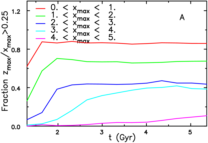
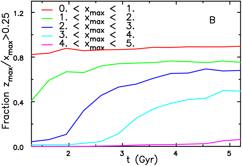
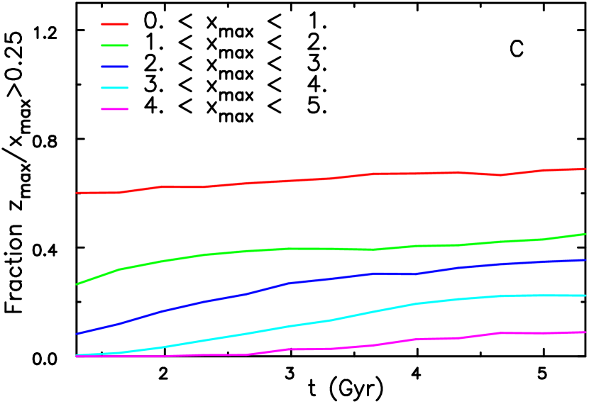
Figure 7: The time evolution of the fraction of orbits in all three models that have $z_{\rm max}/x_{\rm max}>0.25$. The lines are coloured by the extent, in kpc, of the orbits along the bar axis.

4.1 Orbits in an evolving bar

Accordingly, we recorded the position coordinates of a randomly selected fraction of the disc particles at intervals of $0.16\tau_{\rm dyn}\simeq 1\;$Myr. The fraction was 1% in models A and C, and 2% in model B. We also measured the position angle of the bar major axis over time from the mass-weighted average of the $m=2$ sectoral harmonic over the radial range $0.4\leq R\leq 8\;$kpc. For each recorded orbit, we rotated the position about the $z$-axis at each instant to a frame in which the bar position angle is horizontal. Unless otherwaise stated, we selected orbits for which $|x|$ was always $<6\;$kpc for models A and B, and $|x|<8\;$kpc in model C, a criterion that eliminated slightly fewer than half the orbits, which were those that strayed from, or never were in, the bar.

For every orbit, we identified the turning points in each of the separate coordinates $(x,y,z)$ in the bar frame, and computed moving averages of the absolute values at ten successive extrema that bracket a given time, i.e. over five full periods, which we denote $x_{\rm max}(t)$, etc.

Figure 7 plots the time evolution of the fraction of the bar particles in all three models whose greatest vertical departures from the mid-plane $z_{\rm max}/x_{\rm max}>0.25$ at each moment. We separate them by their $x_{\rm max}$ values, in the ranges indicated by the colours. Orbits confined to the inner bar (red line) are nearly all thick, by this criterion, while those that extend into the outer bar (magenta line) are almost all thin, although both lines rise gently with time. For the intermediate ranges, indicated by the green, blue, and cyan lines, the behaviour differs in all three models. In model A, the red, green and blue lines all rise until the buckling instability saturates, while heating in the outer bar (cyan line) is more gradual. The heated fraction also increases substantially in model B, with smaller orbits rising more rapidly early on; both the green and blue lines suggest that $>60$% of the orbits of intermediate values of $x_{\rm max}$ have large $z_{\rm max}/x_{\rm max}$ by the end of the evolution. The heated fractions in model C are generally lower than those in models A and B, which may seem odd, given that the rms thickness was greatest in this bar. However, as noted above, edge-on views in (Fig. 6) reveal that the greater rms thickness in model C is due to low-density halo around the bar, consistent with a smaller heated fraction. (We provide further supporting evidence for this statement in §5.2 below.)

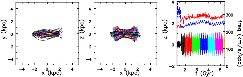
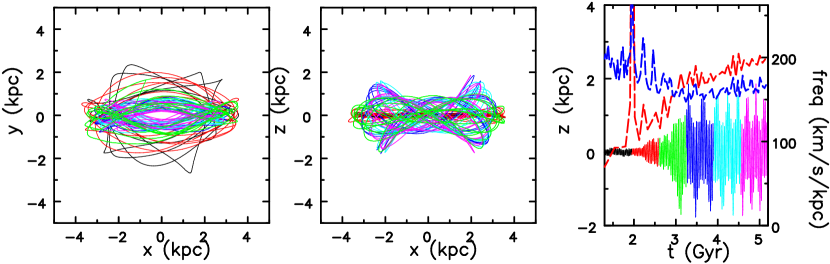
Figure 8: Good examples of vertical heating in models A (above) and B (below). The left and middle panels show $(x,y)$ and $(x,z)$ projections of the orbit in a frame that is oriented at each moment with the bar major axis, which is horizontal. The solid line in the right panel records the time evolution of the $z$ coordinate from $t=1.3\;$Gyr; the colour of this line changes every 0.65 Gyr, as it does in the other two panels, although the black (green) part is plotted last in model A (B). The broken lines in the right panels indicate crude estimates of $2\tilde{\Omega}_{x}$ (red dashed) and $\tilde{\Omega}_{z}$ (blue dashed). In model A (above), the principal increase in the amplitude of the $z$ oscillation occurs at $t\sim 1.7\;$Gyr, which is about when the bar buckles. The frequency changes in model B are more gradual, and heating occurs around the time that the two frequency curves cross, when $2\tilde{\Omega}_{x}\simeq\tilde{\Omega}_{z}$. The subsequent semi-periodic modulation of the vertical oscillation amplitude of both orbits is caused by the turning points of the vertical motion varying with the $x$ position as illustrated in the middle panels.

4.2 Orbit frequencies

Using our recorded orbits in the rotating bar frame, we determined the times at which the motion reversed in each coordinate, and define a rough frequency to be $\tilde{\Omega}_{i}\approx 2\pi/\tilde{\tau}_{i}$, where the period, $\tilde{\tau}_{i}$, is the time between two successive maxima of the particle’s $i$th coordinate, i.e. a full period. Here we use a tilde to distinguish our numerically estimated values from quantities that could be more meaningfully defined through action-angle variables, say. Good examples of orbits from models A and B are illustrated in Figure 8; the two projections in the left and centre panels are drawn in the frame that is rotated at each instant so that the bar major axis is horizontal. The colour of the line in each frame changes with time, as in the right hand panel, although the black (green) part is plotted last in order to show the orbit shape during the period of vertical heating more clearly.

The orbit in model A (above) is heated abruptly as the buckling instability saturates when $\tilde{\Omega}_{z}$, dashed blue curve in the right panel, decreases. Notice that $\tilde{\Omega}_{x}$ also rises at the same moment, because the horizonal extent of the orbit decreases (middle panel).

The $x-y$ projection of the orbit in model B (lower left panel) is elongated parallel to the bar and never approaches the centre, but it does become noticeably skinnier over time. This appearance suggests it is trapped about an $x_{1}$ periodic orbit (see e.g. Sellwood & Wilkinson, 1993) throughout. This in itself is remarkable, since the bar pattern speed decreases by a factor of 2, its amplitude increases by $\ga 30$%, the thickness of the inner bar more than doubles, $\tilde{\Omega}_{z}$ decreases by $\sim 25$%, $\tilde{\Omega}_{x}$ more than doubles, and the $z$-oscillation amplitude increases 10-fold over the period illustrated, yet the basic character of the orbit in its $x-y$ projection scarcely changes! This robust property of the orbit is far from unique – we have noticed similar behaviour in many other orbits.

Our crude frequency estimates are shown by the broken curves in the right panel. Even in a steady potential, the motion of regular orbits (Sellwood & Wilkinson, 1993; Binney & Tremaine, 2008) can be decomposed into librations about an underlying, or parent, periodic orbit. The fundamental frequencies of the parent periodic orbit will generally be incommensurable with the libration frequencies, causing oscillations in all three principal axes to be aperiodic, which is reflected in the short-term variation of the estimated frequencies shown in this Figure.

The frequencies of this orbit also change on a longer time scale as the bar evolves; $\Omega_{z}$ decreases because the bar thickens, reducing the density, while the increase in $\Omega_{x}$ results from the more rapid apparent motion of the particle as the rotating frame of the bar slows. While there is substantial jitter in the individual frequency estimates, the two dashed curves clearly cross near $t=3\;$Gyr, which is about the time of a rapid increase in the vertical oscillation amplitude of this orbit, consistent with the mechanism proposed by Quillen et al. (2014). We will show in §4.4 below that this behaviour is quite general.

The modulation of the $z$ excursions at later times in Figure 8 is another property that occurs in many other orbits, and is accounted for as follows. As may be seen from the $(x,z)$ projection of the orbit in the middle panel, the absolutely largest values of $|z|$ occur when $|x|\ga 2\;$kpc. But $z$ maxima are also reached when $|x|\la 1.6\;$kpc, where the envelope of the orbit in the middle panel has a flattish waist, which must be caused by a stronger vertical restoring force where the mass density is higher. Since $\tilde{\Omega}_{x}$ and $\tilde{\Omega}_{z}$ are generally incommensurable, the vertical oscillation amplitude is modulated as shown, and the increasing difference between the $x$- and $z$-oscillation frequencies after $t\sim 3\;$Gyr results in the observed decreasing modulation period of the $z$-oscillation amplitude. Note that the oscillation amplitude variations appear to have little effect on the estimated vertical frequency (dashed blue curve in the right panel).

Once again, in order to obtain more smoothly varying frequency estimates, we henceforth compute each frequency from moving averages over 10 full periods in each coordinate.

4.3 Collective support for buckling

Particles confined within a bending bar experience a vertical driving acceleration as a result of their horizontal motion along the bar. When the vertical distortion is a single arch, the vertical forcing frequency is twice that of its horizontal frequency along the bar. If this forcing frequency, $2\Omega_{x}$, is less than the natural frequency of free oscillation in the vertical direction, $\Omega_{z}$, then the particle will be able to follow the bend. Any orbit for which $\Omega_{z}<2\Omega_{x}$ would respond out of phase with the bend and would not cooperate with the bending instability. Thus Merritt & Sellwood (1994) argued that a supporting response to a buckling bar, i.e. a collective instability, is expected only for orbits that have $\Omega_{z}>2\Omega_{x}$.

Figure 9: Frequencies, estimated at $t=1.3\;$Gyr, of orbits in model A whose vertical excursions more than doubled at the time the bar buckled. The sizes of the symbols indicate the logarithm of half the factor by which $z_{\rm max}$ has grown over the interval $1.3\pm 0.3\;$Gyr. The line has slope 2 and frequencies are in units of km s^-1 kpc^-1.

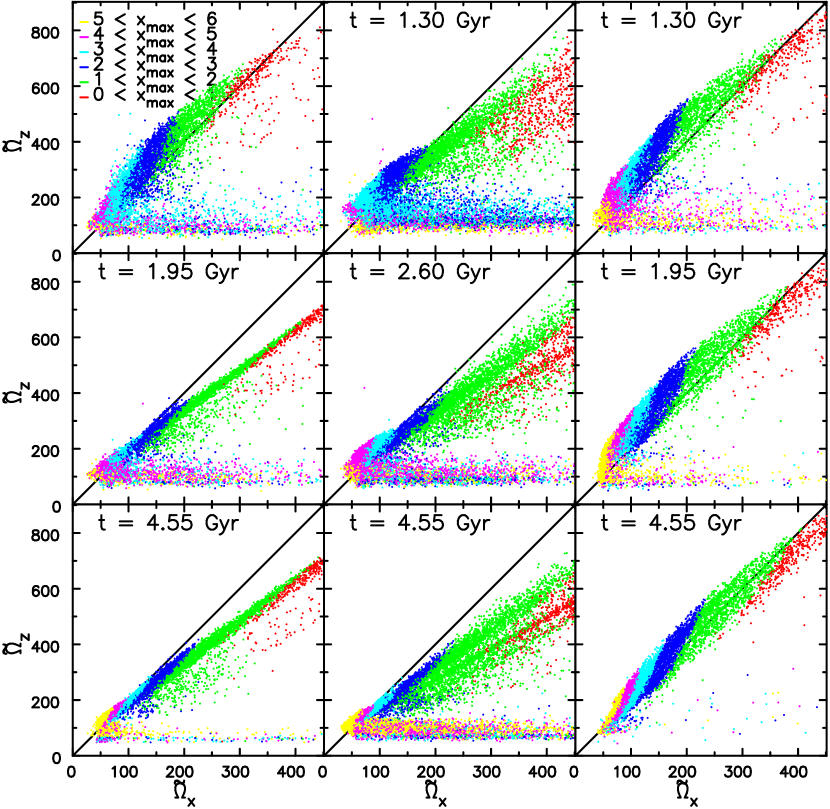
Figure 10: The frequency distribution of all recorded orbits, except those in the far outer disc, in models A (left), B (middle), and C (right) soon after the bar formed (top row), towards the end of the simulation (bottom row), and at an intermediate time (middle row). The diagonal line marks the 2:1 resonance. The approximately horizontal distributions of particles at low $\tilde{\Omega}_{z}$ are mostly outside the bar. The range of $x_{\rm max}$ values in kpc are indicated by the colours.

Figure 9 records the frequencies of orbits in model A for which the magnitude of the vertical excursion more than doubled at the time of the buckling event $t\approx 1.5\;$Gyr. We also selected orbits that were significantly elongated in the direction of the bar, such that $y_{\rm max}<0.3x_{\rm max}$. The frequencies $\tilde{\Omega}_{x}$ and $\tilde{\Omega}_{z}$ were estimated at $t=1.3\;$Gyr, i.e. in the early stages of the bending instability. Almost all these orbits have $\tilde{\Omega}_{z}>2\tilde{\Omega}_{x}$, which is consistent with their need to follow the growing bend of the bar. It is very likely that our frequency estimates were incorrect for the three points that are below the line.

The left-hand panels of Figure 10 report the frequencies of all recorded orbits (see §4.1), excluding only those in the far outer disc, at three different times in model A, and are color coded by ranges of $x_{\rm max}$. The top panel is for the same time as Figure 9 but now includes orbits lying below the resonance line whose vertical oscillation amplitude did not increase over the period of the buckling instability. Particles in the disc outside the bar all have low values of $\tilde{\Omega}_{z}$. Recall that $\tilde{\Omega}_{x}$ is estimated from intervals between $\dot{x}$ reversals; eccentric orbits outside the bar will have irregular shapes when viewed in the bar frame, causing a broad spread in this plotted frequency that has little physical significance.

The middle and bottom left panels of Figure 10 show the same quantities later in the evolution, at $t=1.95\,$Gyr and $t=4.55\,$Gyr respectively, of the same simulation. It is remarkable that the majority of bar orbits at the last time are tightly distributed about a line that has slope $\sim 1.38$ and a non-zero intercept and this arrangement was already in place immediately after the buckling instability had run its course (at $t=1.95\,$Gyr). The vertical frequencies of the orbits have decreased, especially in the inner bar, because it has puffed up, but the fact that the global properties of the bar at the later times are such that there is a tight linear relationship between the vertical and horizontal frequencies of almost all these orbits seems highly significant. Portail et al. (2015) reported the distribution of frequency ratios of particles in their frozen bars had a narrow and non-uniform distribution over the range $1.5\la\tilde{\Omega}_{z}/\tilde{\Omega}_{x}\la 2$ (in our notation) and a similar result was reported by Łokas (2019, her Fig 12), although the fuzzier line in her case seemed to pass through the origin. The non-zero intercept of the linear feature in the bottom left panel of our Figure 10 and closest rational slope of 11/8 makes a resonance explanation seem unpromising; the feature deserves a follow-up study.

Figure 11: The locations of nearly resonant skinny orbits in the plane of $(x_{\rm max},z_{\rm max})$ at five different times in model B. The sizes of the symbols indicate the logarithm of the factor by which $z_{\rm max}$ has grown over the interval $t\pm 0.325\;$Gyr. Distances are in kpc, times in Gyr.

4.4 Gradual vertical heating

As noted above, Quillen et al. (2014) suggested that orbits could also be elevated by becoming trapped in a 2:1 vertical resonance that sweeps outwards as the bar evolves, allowing orbits to be later released from the resonance with an increased vertical oscillation amplitude. The bar in model B thickened without buckling, and we here examine whether their puffing mechanism was indeed responsible for its vertical thickening.

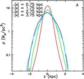
Figure 12: The vertical density profiles at several distances along the bars at the final time. The particles were binned in $\delta x=0.5\;$kpc and only those within $1.6\;$kpc of the bar major axis were included. Notice that while the outer bar in model C has indeed become the thickest, as already noted, the mid-plane density of the inner bar is also the highest.

Figure 13: Two orbits in model C. The description of the panels is as in Figure 8. The orbit in the top row becomes trapped in the vertical resonance, while that is bottom row is not.

In Figure 11, we plot the values of $z_{\rm max}$ against $x_{\rm max}$ of orbits in model B that are close to the resonance, i.e. those for which $|2\tilde{\Omega}_{x}-\tilde{\Omega}_{z}|<4.8\;$km s^-1 kpc^-1. In this Figure, we have included only particles having $y_{\rm max}<0.3x_{\rm max}$, i.e. those whose orbits are highly elongated parallel to the bar. The colours indicate the times at which all these quantities were measured and the sizes of the symbols are proportional to the logarithm of the factor by which $z_{\rm max}$ has grown over an interval of $0.65\;$Gyr that brackets the time of the measurement. The orbits with the larger symbols have been lifted to larger $z_{\rm max}$ by passage through the resonance. The resonance is broad in both $x_{\rm max}$ and $z_{\rm max}$ at any one time, but there is a clear trend that the resonance moves outwards, i.e. to larger $x_{\rm max}$, over time as the bar slows. The anharmonic vertical potential causes the colour bands in Figure 11 to have a positive inclination; this follows because $\Omega_{z}$ decreases with increasing $z_{\rm max}$ at fixed $x_{\rm max}$, which requires a lower $\Omega_{x}$ and thus larger $x_{\rm max}$ to be in resonance.

The symbols of each colour in Figure 11 fill quite broad and overlapping bands, suggesting that the resonance might not be sharp. There are several possible reasons that could cause a real or apparent broadening of the resonance. First, the approximate nature of our frequency estimates will blur the resonance somewhat, although particles that are wrongly identified as being in resonance will not be trapped and therefore should not be elevated, giving rise to small symbols in Figure 11 that are outliers of the distribution of truly resonant orbits of a given colour, as appears to be the case. Second, the time resolution of the color coding is quite coarse and the bar will have evolved over the interval spanned by each colour, causing a true spread in the location of the resonance. Third, orbits having the same values of $(x_{\rm max},z_{\rm max})$ at a given time could have differing shapes: some will be skinny, i.e. have small $y_{\rm max}$, while others will be rounder, and whether they are in resonance will depend somewhat on their shape. To test this idea, we examined resonant orbits for which $y_{\rm max}>0.3x_{\rm max}$, i.e. rounder orbits in the bar frame, finding that the rounder orbits had a distribution in Figure 11 that was about twice as broad as the skinnier orbits, confirming this hypothesis. A fourth reason could be that the resonance is intrinsically quite broad because of the large potential perturbation caused by the strong bar.

The bar in model A continued to thicken after the buckling event (Figure 2d). We have similar evidence from this case to that in model B (Figure 11), but do not present it, that the secular thickening in this bar happened by the Quillen et al. (2014) mechanism, since the orbits that were nearly resonant $|2\tilde{\Omega}_{x}-\tilde{\Omega}_{z}|<4.8\;$km s^-1 kpc^-1 were raised by the largest factors, and again we observed the resonance moving gradually out along the bar.

The middle panels of Figure 10 show the frequencies of all orbits in model B at $t=1.3\,$Gyr (top), $t=2.6\,$Gyr (middle), and $t=4.55\,$Gyr (bottom). The addition of the nuclear star cluster in model B should have raised the values of both frequencies in the inner bar, shifting the points up and to the right in comparison with model A, although the surface density in the inner bar in B had not risen as much as in A because the bar was not quite fully formed at this time. However, it is clear that few of the red and green points in model B, particles within 2 kpc of the centre, lie above the diagonal at the earlier time. This is the reason that the bar did not buckle (see the discussion in §4.3). When the bar had settled and begun to puff up ($t=2.6\;$Gyr), the high frequency orbits, in the inner bar, lie farther below the diagonal line, as for model A, and in both runs one can see that those orbits that remain in resonance at the later time are low-frequency orbits in the outer bar, confirming in a different way that the resonance has swept outwards along the bar to lower frequencies.

It is instructive to compare the evolution of the thicker fraction in Figure 7(B) with the changes between the top and bottom panels for the same model B in Figure 10. (Note that the colour codes for $x_{\rm max}$ are the same in both figures.) The fraction of particles that are heated to larger $z_{\rm max}$ rises later in the evolution at larger radii, and these particles can be seen to lie below the resonance line in the bottom middle panel of Figure 10; the only orbits still in resonance at this time are in the outer bar ($x_{\rm max}\ga 3$). Thus, we consider this evidence, combined with that in Figure 11, to indicate clearly that the bar in model B thickened as the resonance swept out along the bar (Quillen et al., 2014).

The distribution of particles in frequency space in bottom middle panel of Figure 10 (model B), has bifurcated into two features: a broader version of the line in model A and a sharp line having a shallower slope $\sim 1$ and a non-zero intercept. Perhaps even a third line having a yet shallower slope is faintly discernible. Once again, we defer this unexpected finding to a follow-up investigation.

4.5 Trapping into resonance

The behaviour in model C is different from that in both models A and B, as may be seen in the right-hand panels of Figure 10. The similarity of the diagrams for models A and C at $t=1.3\;$Gyr is because model C differed from model A only by the imposition of vertical symmetry, which inhibited the buckling instability that was on-going in model A at this time. But in the middle and bottom panels almost all particles in model C have remained close to the resonance line, whereas the distribution in model A (bottom left) is narrower and has a different slope and intercept. Thus it seemed possible that many bar particles in model C had been trapped into the 2:1 vertical resonance. Indeed, Quillen (2002) had proposed this as a mechanism for bar thickening, but we are unaware of any previously reported simulation that supported her suggestion.

It may seem puzzling that the $\tilde{\Omega}_{z}$ values in the inner bar are higher at the later time than in the other bars, even though this bar thickened more. However, we noted above that the disc in model C gave up over 30% of its angular momentum to the halo, mostly from the inner disc, which allowed particles to settle closer to the centre thereby creating a higher density in the bar than in model A. This is illustrated in Figure 12, which compares the vertical density profiles of all three bars at a range of $x$-distances from the bar centre. It can be seen that the mid-plane density of the inner bar in model C is the highest of the three bars. Thus the vertical restoring forces in the inner bar of model C are stronger than those in model A, causing higher vertical frequencies.

The orbit presented in the top row of Figure 13 is a good example of orbit trapping in model C, illustrating that once an orbit gets into approximate resonance, it remains there for the duration of the simulation. That in the bottom row is not trapped by the end of the simulation. The later gradual rise of both frequencies, visible in the rightmost panels, is due to the increasing density in the inner bar as the model evolves. Furthermore, the vertical oscillation amplitude of the trapped orbit does not increase monotonically, but fluctuates about a mean that is generally much greater than its initial vertical amplitude, whereas the orbit that is not trapped is not heated. There are many orbits of both types in the bar of model C.

The colour bands at the intermediate and later times in the right hand panels of Figure 10 are quite sharp because the range of $x_{\rm max}$ largely determines the horizontal frequency of the orbit in the bar potential. The boundaries between the colours have positive slope, indicating that those with higher vertical frequency or equivalently smaller vertical excursions, have slightly higher horizontal frequencies at the same $x_{\rm max}$.

The distribution about the diagonal in the bottom, right panel of Figure 10 is much broader than that of the line in the bottom left panel, suggesting that the width is mostly intrinsic, and not simply measuring errors in the frequencies, a point that is supported by the sharpness of the boundaries of the colour bands. However, not all the particles are resonant, as was illustrated by the two examples in Figure 13, and the non-resonant particles, which have not been heated, are generally above the diagonal. Orbits are heated as they become trapped, which causes $\tilde{\Omega}_{z}$ to decrease.

Notice that there are very few green or blue points far below the diagonal in the bottom right panel of Fig. 10, implying that most heated orbits remain trapped. We have found that $\sim 10$% of orbits that were heated later have persisting frequencies below the resonance condition, suggesting they may have escaped from the resonance. However, the small frequency differences in some cases make it difficult to be certain that all such orbits have fully escaped.

It should be emphasized that model C is artificial, because we imposed reflection symmetry about the mid-plane throughout its evolution. It is therefore possible that this third mechanism for bar thickening may arise solely in simulations having this unphysical constraint.

5 Discussion of the thickening mechanisms

The distributions of points in all three panels in the top row of Figure 10 include many particles lying close to the resonance line before the bar thickened. It may therefore seem that the resonance played a role in thickening all three bars and that the diverging behaviour of each of the three models reflected different consequences of the same underlying mechanism.

In order to show that this is not the case, we present two additional simulations in which the initial disc thickness was halved to $z_{0}=100\;$pc, but which were otherwise identical to models A and C. We denote these models as A₁₀₀ and C₁₀₀, respectively with the subscript indicating the vertical scale of the initial disc. Doubling the disc density in this way strengthens the gravitational attraction both vertically towards the mid-plane and in the radial direction, particularly near the disc centre.

The first consequence of this change is that the bar instability is a little more vigorous. The bar in model A₁₀₀ formed by $t\sim 0.5\;$Gyr and buckled around $t\sim 1.4\;$Gyr, as shown in Figure 14, a little earlier than in model A. After buckling, the evolution of the bar in model A₁₀₀ resembled that in A, shown in Fig. 2, in length, amplitude, pattern speed, and thickness (despite having started from a thinner disc).

The bar in model C₁₀₀ formed at the same time as that in model A₁₀₀, as expected, but its subsequent evolution was not as extreme as that in model C. It neither became as strong, nor as long, nor did it slow down or puff up to the same extent as shown in Fig. 5. In this case the halo gained $\sim 22$% of the initial disc angular momentum, which is still a substantial fraction, but considerably less than in model C over the same interval.

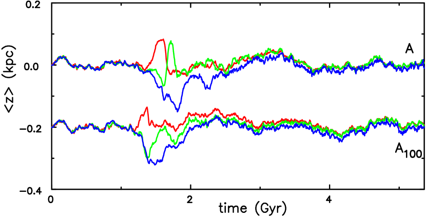
Figure 14: As for Fig. reffig.zbend but for models A (reproduced from Fig. 3) and A₁₀₀. Values for model A₁₀₀ have been shifted by $-200$ pc for clarity.

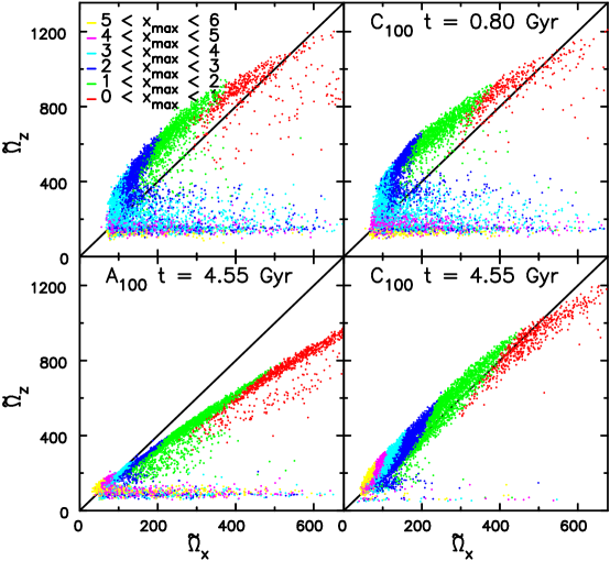
Figure 15: As for Fig. 10 but for models A₁₀₀ (left) and C₁₀₀ (right). The frequency ranges have been increased and the top row is for $t=0.8\;$Gyr.

5.1 Buckling instability

Figure 15 presents the distributions in frequency space of the particles in models A₁₀₀ (left) and C₁₀₀ (right), at $t=0.8\;$Gyr (top) and $t=4.55\;$Gyr (bottom). Notice that the frequency ranges have been increased in comparison with those of Fig. 10. Most points from particles within the bar ($x_{\rm max}\leq 3\;$kpc) in both both models now lie well above the 2:1 resonance line (marked by the diagonal), yet the bar in model A₁₀₀ buckled in the same manner as in model A. As argued in §4.3 above, and originally by Merritt & Sellwood (1994), the collective instability requires that most particles have $\Omega_{z}>2\Omega$, and this condition is still true in model A₁₀₀ even though the particle distribution in model A₁₀₀ is clearly farther from the resonance line in A₁₀₀ than it is in A. Thus the buckling instability does not require bar particles to be close to the 2:1 vertical resonance as was also illustrated for a single orbit in the upper right panel of Fig. 8.

It is also noteworthy that the distribution of points in the lower left panel of Figure 15 (model A₁₀₀) again is strongly concentrated in a line of similar slope and intercept as that in the lower left panel of Figure 10 (model A) although now with a wider frequency range.

5.2 Resonance passage vs resonance capture

While it is true that the 2:1 vertical resonance plays a pivotal role in the thickening of the bars in both models B and C, the mechanisms are quite distinct. Quillen et al. (2014) noted this distinction, but argued that the trapping mechanism proposed by Quillen (2002) was unlikely to be of importance because “the resonance width was too narrow”. We presented compelling evidence in §4.4 that particles in model B were heated vertically as the resonance swept past them (Quillen et al., 2014).

The behaviour in model C is quite different. Figure 7(C) shows the time evolution of the fraction of vertically heated orbits in model C. The heated fractions are generally lower than in model B, consistent with the differing density profiles (Fig. 12). But the more interesting contrast with Fig. 7(B), is that the bar particles in model C were heated almost continuously at all radii. Thus there is no evidence that the resonance was sweeping outwards along the bar, but instead vertical heating by capture into resonance was happening steadily at all $x_{\rm max}$. Note that vertical heating began for $x_{\rm max}>3$ (cyan) and $>4\;$kpc (magenta) at later times because the bar grew in length over time (Fig. 5(b)). Particles were heated vertically as they became trapped, and the fraction of trapped orbits increased continually to the end of the simulation. Thus we have found a case in which the 2:1 resonance extends over a large part of the bar that seems consistent with the original suggestion in Quillen (2002).

The mid-plane density in the bar of model C was high enough to hold the particles in resonance, once captured. The lower density in model B, prevented particles in the inner bar from remaining in resonance.

As noted above, the evolution of the bar in model C₁₀₀ differed significantly from that in C, yet the distribution of particles in frequency space in the bottom right panel of Figure 15 again straddles the diagonal to about the same extent as it did in the lower right panel of Figure 10, albeit over a slightly more extensive frequency range in this new case. Visual examination of the orbits of particles in model C₁₀₀ again revealed that an increasing fraction particles within the bar held the ratio $\Omega_{z}\simeq 2\Omega_{x}$, after it was reached, also suggesting that they had become trapped into the 2:1 vertical resonance.

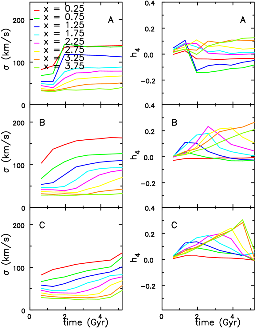
Figure 16: The time evolution of the vertical velocity distributions of particles having $|z|<200\;$pc in the bars of model A (top) that did buckle, model B (middle) that did not buckle, and model C (bottom) in which buckling was suppressed. The left panels show the dispersion $\sigma$ and the right the coefficient $h_{4}$. The colours code the measurements in bins of different $x$, with the indicated mean values in kpc, and particles lying at distances from the bar major axis $y>1.6\;$kpc have also been excluded.

6 Comparison with observations

The bars in models A and B puffed up by different mechanisms: a secular resonant trapping process for lifting orbits in model B and a dynamical buckling instability in model A, although secular thickening continued after the buckling instability had run its course. The final bars in these two cases are quite similar, as summarized in Figures 2 and 4. The bar in model B is slightly weaker (panels a), shorter (panels b) and not quite so thick (panels d) as that in model A, but their pattern speeds (panels c) and thickness profiles (panels d) were remarkably similar. Also, the overall thickening process occurs over similar periods, even though the rapid surge associated with the saturation of the buckling instability in model A, differs from the more gradual thickening in model B. A more significantly different bar developed in model C, that also thickened by a third mechanism: resonant trapping.

With the objective to find fossil evidence in the velocity distribution that could allow a bar that buckled to be distinguished from one that did not, we have computed the coefficients $h_{3}$ and $h_{4}$ of a Gauss-Hermite expansion (Gerhard, 1993; van der Marel & Franx, 1993) of the vertical velocity distribution. A non-zero value of $h_{3}$ would reflect a skew velocity distribution, a positive value of $h_{4}$ indicates a velocity distribution that is more peaked than a Gaussian and also has heavier tails, while the distribution is more flat topped with weaker tails when $h_{4}<0$.

We binned bar particles in slices of $|z|$-height, and in $|x|$-distance along the bar, and determined these coefficients from the particle velocities in each bin as described in the Appendix.

The results of this analysis for particles with $|z|<200\;$pc are presented as functions of time in Figure 16. The gradual rise of $\sigma$ in models B and C, compared with the sudden surge for $x\la 2\;$kpc between $1.3\leq t\leq 1.95\;$Gyr in model A, reflects the thickening histories already presented in Figs. 2, 4, and 5. We do not show the evolution of $h_{3}$, because it remained near zero in all three models. However, there are clear differences in $h_{4}$: on the one hand, the $h_{4}$ values in models B and C (middle and bottom rows) tend to be positive, and one can observe the peak in $h_{4}$ gradually shifting to larger distance from the centre, with values declining at each radius as the peak moves farther out. On the other hand, the buckling event in model A (top row) causes $h_{4}$ to become strongly negative for $0.5\leq|x|\leq 2\;$kpc (green and blue lines), as was also reported by Debattista et al. (2005), although the values in these bins subsequently trend back towards zero gradually over time. Farther out in the bar of model A, the behaviour more closely resembles that in model B, reflecting the continued puffing up of the bar, after the buckling event, by the resonance trapping mechanism at later times.

These systematic differences between the $h_{4}$ values can be traced to larger height above and below the mid-plane, although trends weaken and the differences merge into the noise for $|z|\ga 500\;$pc.

These differences must be consequences of differences in the vertical density profile of the bar. When $h_{4}>0$, the velocity distribution is more peaked than a Gaussian, and also has a heavy tail of high velocity stars, which seems likely to reflect a vertical density profile having a “core-halo” structure. Conversely, the density profile will be more truncated with height when $h_{4}<0$. Figure 12 presents the vertical density profiles in the bars at the end of the evolution ($t=5.2\;$Gyr) in all three models. The density profile in model C near $|x|\sim 3.75\;$kpc has heavy tails (cyan curve) where $h_{4}>0$, whereas it drops off more steeply with height in models A and B near $|x|\sim 1.75\;$kpc when $h_{4}<0$ (green curves), as expected from this argument.

We have verified that this same difference reflects the thickening mechanisms in other models. In particular, we have found strongly negative values of $h_{4}$ near where the buckling instability produced the peanut shape in another case, not presented here. Even though the $h_{4}$ values had all relaxed to near zero by the end of the evolution in that model, the behaviour still contrasts with the large positive values at some radii in the bars that puff up more gradually.

6.1 Comparison with Milky Way

We suggest that the sign and radial variation of the $h_{4}$ coefficient of the vertical velocity distribution could be used as fossil indicator of a bar that has buckled in its history. In particular, the values of $h_{4}$ for the vertical velocity distribution of stars in the Milky Way could be used to test whether the bar in our Galaxy has buckled in the past. However, we defer this test to a second paper, since extracting this information from the proper motions of the red-clump giants of the Virac-Gaia survey (Smith et al., 2018; Clarke et al., 2019) requires a detailed discussion.

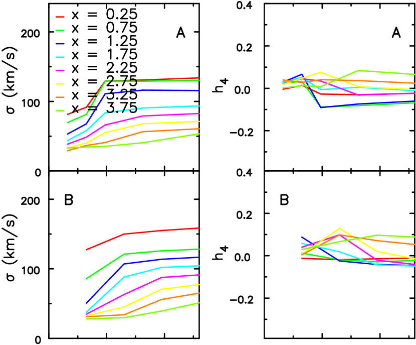
Figure 17: The time evolution of the $z$-projected vertical velocity distributions of particles near the major axis of the bars of model A (above) that did buckle and model B (below) that did not buckle. The dispersion $\sigma$ is shown in the left panel and the coeffificent $h_{4}$ on the right. The colours code measurements in bins of different $x$ distances along the bar, with the indicated mean values in kpc, and particles lying at distances from the bar major axis $y>0.4\;$kpc are eliminated.

6.2 Comparison with external galaxies

The data presented in Fig 16 were for comparison with the Milky Way, but we can also make predictions for projected velocity distributions such as might be observed in external galaxies. Méndez-Abreu et al. (2008) took long-slit spectra of two face-on barred galaxies, and compute a Gauss-Hermite fit to the absorption line profiles. We therefore show in Fig 17 the $z$-projected velocity distribution of models A and B using a pseudo-slit of half-width 400 pc; the different colours are for different $x$-distances along the bar. Since the particle density is highest near the mid-plane, it is no surprise that signal in the $h_{4}$ coefficients is only slightly weaker than those from the mid-plane only, shown in Fig 16.

For NGC 98, Méndez-Abreu et al. (2008) found negative values of $h_{4}$ out to 5″ from the centre along the bar major axis and concluded, on the basis of comparison with simulations by Debattista et al. (2005), that the bar had buckled. Our findings would support their conclusion. However, they reported positive values of $h_{4}$ in the case of NGC 600, for which they offered no explanation. Our models would suggest that if the bar in that galaxy has thickened (Erwin & Debattista, 2013, suggest it may not have), it might have resulted from resonance heating.

7 Conclusions

We have presented simulations of bar formation and evolution in idealized models of a disc embedded in a spherical halo. In most models, the evolution was computed self-consistently, but we have also presented cases in which the potential was constrained throughout to remain reflection symmetric about the mid-plane in order to suppress the buckling instability. The bars in all our models thickened, but by three different mechanisms.

A buckling instability in a two-component disc-halo model caused some of the thickening when the evolution was unrestricted. We found that adding a nuclear star cluster in the centre, having just 2.5% of the disc mass, seemed sufficient to suppress the buckling instability. We have presented substantial evidence that the bar in this case puffed up because the $z$-excursions of orbits were increased as a 2:1 vertical resonance swept out along the bar, as was elegantly described by Quillen et al. (2014). Particles were heated as they became resonant, and the increased amplitude of their vertical motion persisted after they left the resonance.

We have also uncovered a third thickening mechanism: gradual trapping into the 2:1 vertical resonance. In this mechanism, particles all along the bar were heated as they become captured into the resonance, where they remained until the end of the simulation. Quillen (2002) had proposed this as a thickening mechanism, but no example has previously been claimed, to our knowledge. Note that we have observed this mechanism only in our vertically symmetrized models, but it may possibly also occur in unrestricted models having different initial conditions.

We have reported only a few simulations, in which we have identified the three different thickening mechanisms, but we have run many more and have not noticed a fourth thickening mechanism among them. However, we cannot exclude the possibility that other bars might thicken by as yet undiscovered means.

Since we are unable to observe the evolution of any individual galaxy, the mechanism by which the bar thickened can be deduced only from fossil evidence (unless the bar is observed directly in the short buckling phase, as was claimed by Erwin & Debattista, 2016). We have found clear evidence that the Gauss-Hermite coefficient $h_{4}$ of the vertical velocity distribution provides such fossil evidence of a bar’s dynamical history: it is negative in the inner regions of a buckled bar, as previously found by Debattista et al. (2005), but here we show that it is positive when the bar has been puffed up by either of the two more gradual mechanisms. We caution that we have found this distinction in rather few bar models, and so cannot say that it is completely general.

Méndez-Abreu et al. (2008) present evidence for negative $h_{4}$ values from the vertical velocity distribution of the face-on bar of NGC 98, which they argued was evidence that the bar had buckled. But they also found positve $h_{4}$ values in NGC 600; if the bar in this galaxy has puffed up, our work suggests that the mechanism proposed by Quillen et al. (2014) could be responsible.

We are currently applying this diagnostic to the vertical velocity distribution of stars in the Milky Way bulge, which will the subject of a subsequent paper.

Appendix

van der Marel & Franx (1993) and Gerhard (1993) noted that a non-Gaussian line profile may be described as a Gauss-Hermite series

$${\cal L}(v)=\left[{A\alpha(w)\over\sigma}\right]\sum_{k}h_{k}H_{k}(w),\qquad\hbox{where}\qquad w={v-V\over\sigma}.$$ (4)

Here, the standard Gaussian function $\alpha(w)=\exp(-w^{2}/2)/\sqrt{2\pi}$, $V$ and $\sigma$ are the mean and dispersion of the best fitting Gaussian, and $A$ is its normalization. The functions $H_{k}(w)$ are Hermite polynomials, and the coefficients $h_{k}$ are free parameters. When $\alpha$ is defined in this standard way, the first seven polynomials are

$$H_{0}(w)=1,\qquad H_{1}(w)=\sqrt{2}w, H_{2}(w)=(2w^{2}-1)/\sqrt{2},$$

$$H_{3}(w)=(2w^{3}-3w)/\sqrt{3}, H_{4}(w)=(4w^{4}-12w^{2}+3)/\sqrt{24},$$ (5)

$$H_{5}(w)=(4w^{5}-20w^{3}+15w)/\sqrt{60}, H_{6}(w)=(8w^{6}-60w^{4}+90w^{2}-15)/\sqrt{720}.$$ and

These expressions are normalized such that $\int_{-\infty}^{\infty}\alpha(w)H_{k}(w)\;\alpha(w)H_{m}(w)\;dw=\delta_{km}(4\pi)^{-1/2}$, where $\delta_{km}$ is the Kronecker delta, in agreement with eq. (6) of van der Marel & Franx (1993). Since these functions are orthogonal, the coefficients $h_{k}$ in eq. (4) are independent of each other.

Following van der Marel & Franx (1993), we hold $(h_{0},h_{1},h_{2})$ fixed to to $(1,0,0)$, while allowing $(A,V,\sigma)$ to be free parameters of the fit to the generalized profile; Magorrian & Binney (1994) prove that this simplification does not alter the fit. Thus, a fit to the line profile for $k\leq 4$ has the functional form

$${\cal L}(v)=\left[{A\alpha(w)\over\sigma}\right]\left\{1+h_{3}H_{3}(w)+h_{4}H_{4}(w)\right\},$$ (6)

with five free parameters: $(A,V,\sigma,h_{3},h_{4})$.

It should be noted that the function (6) becomes negative over some range(s) of $v$ for any non-zero value of $h_{3}$ and all but small positive values of $h_{4}$. When both coefficients have small absolute values, the range(s) where the function is negative is (are) out in the wings of the profile where the Gaussian factor causes negative values of the function to have little significance. However, when fitting this function to the velocity distribution of particles, the values of $h_{3}$ and $h_{4}$ will be constrained by the fact that the function to be fitted is nowhere negative.

We could construct an “observed” line profile, ${\cal L}_{0}(v)$ from the velocity distribution of a finite number of particles, and then try to fit the expression (6) to it by a least squares minimization for ${\cal S}_{\rm s}=\sum_{j}\left[{\cal L}_{o}(v_{j})-{\cal L}(v_{j})\right]^{2}$, at some set of velocities $\{v_{j}\}$. This would be undesirable, however, because we would need to define a smooth function ${\cal L}_{o}(v)$ through a kernel estimate, for example, which would immediately introduce a bias.

Fitting the cumulative velocity distribution avoids this particular bias. (The values of $h_{3}$ and $h_{4}$ will continue to be constrained by the always increasing cumulative distribution). The integral of the line profile (6) to velocity $v$, or to $w$, is

$${\cal N}(v) = \int_{-\infty}^{v}{\cal L}(v^{\prime})\;dv^{\prime}={A\over\sigma}\int_{-\infty}^{w}\alpha(w^{\prime})\left\{1+h_{3}H_{3}(w^{\prime})+h_{4}H_{4}(w^{\prime})\right\}dw^{\prime}$$ (7)

$$= {A\over\sigma}\left\{Q_{0}(w)+{h_{3}\over\sqrt{3}}\left[2Q_{3}(w)-3Q_{1}(w)\right]+{h_{4}\over\sqrt{24}}\left[4Q_{4}(w)-12Q_{2}(w)+3Q_{0}(w)\right]\right\}.$$

Since $\hbox{erf}\,(x)\equiv(2/\pi^{1/2})\int_{0}^{x}e^{-t^{2}}dt$, we find

$$Q_{l}(w)=\int_{-\infty}^{w}w^{\prime l}\alpha(w^{\prime})\;dw^{\prime}=\begin{cases}\displaystyle{1\over 2}\left[1+\hbox{erf}\,\left({w\over\surd 2}\right)\right]&l=0\\ -\alpha(w)\phantom{\displaystyle{1\over 2}}&l=1\\ \displaystyle{1\over 2}\left[1+\hbox{erf}\,\left({w\over\surd 2}\right)\right]-w\alpha(w)&l=2\\ -\alpha(w)\left(w^{2}+2\right)\phantom{\displaystyle{1\over 2}}&l=3\\ \displaystyle{3\over 2}\left[1+\hbox{erf}\,\left({w\over\surd 2}\right)\right]-w\alpha(w)\left(w^{2}+3\right).&l=4\\ \end{cases}$$ (8)

The expression for $Q_{0}$ is standard, the integrals for $l=1$ and $l=3$ are easy, while those for $l=2$ and $l=4$ must be integrated by parts with the help of formula 5.41 from Gradshteyn & Ryzhik (1980).

Now assume we have a set of $n$ discrete velocities, $\{v_{i}\}$. The cumulative distribution of the input data to be fitted is therefore

$${\cal N}_{o}(v_{i})={1\over n}\sum_{j=1}^{n}H(v_{i}-v_{j}),$$ (9)

where the Heaviside function $H(v_{i}-v_{j})=1$ if $v_{i}\geq v_{j}$ and $H(v_{i}-v_{j})=0$ otherwise. The best fit line profile is that for which the five parameters $(A,V,\sigma,h_{3},h_{4})$ have the values that minimize

$${\cal S}_{\rm u}=\sum_{i=1}^{n}\left[{\cal N}_{o}(v_{i})-{\cal N}(v_{i})\right]^{2}.$$ (10)

Clearly, $A/\sigma$ must be close to unity, because of the normalization of ${\cal N}_{o}$ in eq. (9). We use the fitting tool, sumsl, (from the software collection made public by Burkardt, 2017) that finds the set of five parameters $\{p_{j}\}$ that minimize ${\cal S}_{\rm u}$. Note that this tool requires a routine to supply a vector of gradients $\{\partial{\cal S}_{u}/\partial p_{j}\}$ at any point on the hyper-surface.

As a measure of the goodness of the fit, we use a Kolmogorov-Smirnov test to estimate the probability that the data $\{v_{i}\}$ were drawn from the fitted distribution ${\cal N}(v)$.

It might be objected that the integrated Hermite polynomials $\int_{-\infty}^{w}\alpha(w^{\prime})H_{k}(w^{\prime})\;dw^{\prime}$ are not orthogonal, and the coefficients $h_{k}$ will therefore no longer be independent. Although this is true, we find the best fit values of $h_{3}$ and $h_{4}$ derived by minimizing ${\cal S}_{\rm u}$ using the unsmoothed cumulative distribution agree quite well with those obtained from minimizing ${\cal S}_{\rm s}$ to the smoothed data. The main source of difference is that smoothing reduces the magnitude of $h_{3}$ and $h_{4}$, as is to be expected. In all cases that we have examined, the KS probability that the values were drawn from the fitted distribution were higher for the cumulative fit than for the fit to the smoothed “line profile.”

References

- Abbott et al. (2017) Abbott, C. G., Valluri, M., Shen, J. & Debattista, V. P. 2017, MNRAS, bf 470, 1526
- Aguerri et al. (2015) Aguerri, J. A. L., Méndez-Abreu, J., Falcón-Barroso, J., et al. 2015, A&A, 576, A102
- Binney, Gerhard & Spergel (1997) Binney, J., Gerhard, O. & Spergel, D. 1997, MNRAS, 288, 365
- Binney & Tremaine (2008) Binney, J. & Tremaine, S. 2008, Galactic Dynamics 2nd Ed. (Princeton: Princeton University Press)
- Bland-Hawthorn & Gerhard (2016) Bland-Hawthorn, J. & Gerhard, O. 2016, ARA&A, 54, 529
- Bureau & Athanassoula (2005) Bureau, M. & Athanassoula, E. 2005, ApJ, 626, 159
-
Burkardt (2017)
Burkardt, J. 2017,
Website: https://people.sc.fsu.edu/jburkardt/ - Clarke et al. (2019) Clarke, J. P., Wegg, C., Gerhard, O., Smith, L., Lucas, P. & Wylie, S. 2019, MNRAS, 489, 3519
- Colin & Athanassoula (1989) Colin, J. & Athanassoula, E. 1989, A&A, 214, 99
- Collier (2020) Collier, A. 2020, MNRAS, 492, 2241
- Combes et al. (1990) Combes, F., Debbasch, F., Friedli, D. & Pfenniger, D. 1990, A&A, 233, 82
- Combes & Sanders (1981) Combes, F. & Sanders, R. H. 1981, A&A, 96, 164
- Dame, Hartmann & Thaddeus (2001) Dame, T., Hartmann, D. & Thaddeus P. 2001. ApJ, 547, 792
- Debattista et al. (2005) Debattista, V. P., Carollo, C. M., Mayer, L. & Moore, B. 2005, ApJ, 628. 678
- Debattista & Sellwood (2000) Debattista, V. P. & Sellwood, J. A. 2000, ApJ, 543, 704
- de Vaucouleurs & Freeman (1972) de Vaucouleurs, G. & Freeman, K. C. 1972, Vistas Astron., 14, 163
- Díaz-García et al. (2016) Díaz-García, S., Salo, H., Laurikainen, E. & Herrera-Endoqui, M. 2016, A&A, 587, A160
- Erwin (2018) Erwin, P. 2018, MNRAS, 474, 5372
- Erwin & Debattista (2013) Erwin, P. & Debattista, V. P. 2013, MNRAS, 431, 3060
- Erwin & Debattista (2016) Erwin, P. & Debattista, V. P. 2016, ApJ, 825, L30
- Erwin & Debattista (2017) Erwin, P. & Debattista, V. P. 2017, MNRAS, 468, 2058
- Friedli & Pfenniger (1990) Friedli, D. & Pfenniger, D. 1990, in “Bulges of Galaxies”, eds. B. J. Jarvis & D. M. Terndrup (Garching: ESO workshop 35) p. 265
- Fux (1999) Fux, R. 1999, A&A, 345, 787
- Gajda et al. (2016) Gajda, G., Łokas, E. L. & Athanassoula, E. 2016, ApJ, 830, 108
- Gerhard (1993) Gerhard, O. E. 1993, MNRAS, 265, 213
- Gradshteyn & Ryzhik (1980) Gradshteyn, I. S. & Ryzhik, I. M. 1980, Table of Integrals, Series, and Products 4th Ed. (Orlando: Academic Press Inc.)
- Hammersley et al. (2000) Hammersley, P. L,, Garzón, F,, Mahoney, T.J., López-Corredoira, M. & Torres, M.A.P. 2000, MNRAS, 317, L45
- Hernquist (1990) Hernquist, L. 1990, ApJ, 356, 359
- Holmes et al. (2015) Holmes, L., Spekkens, K., Sánchez, S. F., et al. 2015, MNRAS, 451, 4397
- Howard et al. (2009) Howard, C. D., Rich, R. M., Clarkson, W., et al. 2009, ApJ, 702, L153
- Kormendy (1983) Kormendy, J. 1983, ApJ, 275, 529
- Kuijken & Merrifield (1995) Kuijken, K. & Merrifield, M. R. 1995, ApJ, 443, L13
- Laskar (1990) Laskar, J. 1990, Icar., 88, 266
- Li et al. (2016) Li, Z., Gerhard, O., Shen, J., Portail, M. & Wegg, C. 2016, ApJ, 824, 13
- Łokas (2019) Łokas, E. L. 2019, A&A, 629, A52
- Lütticke, Dettmar & Pohlen (2000) Lütticke, R., Dettmar, R.-J. & Pohlen, M. 2000, A&AS, 145, 405
- Magorrian & Binney (1994) Magorrian, J. & Binney, J. 1994, MNRAS, 271, 949
- Martinez-Valpuesta & Shlosman (2004) Martinez-Valpuesta, I. & Shlosman, I. 2004, ApJ, 613, L29
- Martinez-Valpuesta et al. (2006) Martinez-Valpuesta, I., Shlosman, I. & Heller, C. 2006, ApJ, 637, 214
- McWilliam & Zoccali (2010) McWilliam, A. & Zoccali, M. 2010, ApJ, 724, 1491
- Méndez-Abreu et al. (2008) Méndez-Abreu, J., Corsini, E. M., Debattista, Victor P., De Rijcke, S., Aguerri, J. A. L. & Pizzella, A. 2008, ApJ, 679, L73
- Merritt & Sellwood (1994) Merritt, D. & Sellwood, J. A. 1994, ApJ, 425, 551
- Ness & Lang (2016) Ness, M. & Lang, D. 2016, AJ, 152, 14
- Petersen et al. (2016) Petersen, M. S., Weinberg, M. D. & Katz, N. 2016, MNRAS, 463, 1952
- Petersen et al. (2019a) Petersen, M. S., Weinberg, M. D. & Katz, N. 2019a, arXiv:1902.05081
- Petersen et al. (2019b) Petersen, M. S., Weinberg, M. D. & Katz, N. 2019b, MNRAS, 490, 3616
- Portail et al. (2017) Portail, M., Gerhard, O., Wegg, C. & Ness, M. 2017, MNRAS, 465, 1621
- Portail et al. (2015) Portail, M., Wegg, C. & Gerhard, O. 2015, MNRAS, 450, L66
- Quillen (2002) Quillen, A. C. 2002, AJ, 124, 722
- Quillen et al. (2014) Quillen, A. C., Minchev, I., Sharma, S., Qin, Y-J. & Di Matteo, P. 2014, MNRAS, 437, 1284
- Raha et al. (1991) Raha, N., Sellwood, J. A., James, R. A. & Kahn, F. D. 1991, Nature, 352, 411
- Rangwala et al. (2009) Rangwala, N., Williams, T. B. & Stanek, K. Z. 2009, ApJ, 691, 1387
- Sanders et al. (2019) Sanders, J., Smith, L., Evans, N. W. & Lucas, P. 2019, MNRAS, 487, 5188
- Sellwood (1989) Sellwood, J. A. 1989, MNRAS, 238, 115
- Sellwood (2014) Sellwood, J. A. 2014, arXiv:1406.6606 (on-line manual: http://www.physics.rutgers.edu/sellwood/manual.pdf)
- Sellwood & McGaugh (2005) Sellwood, J. A. & McGaugh, S. S. 2005, ApJ, 634, 70
- Sellwood & Merritt (1994) Sellwood, J. A. & Merritt, D. 1994, ApJ, 425, 530