Cat states in a driven superfluid: role of signal shape and switching protocol

Abstract

We investigate the behavior of a one-dimensional Bose-Hubbard model whose kinetic energy is made to oscillate with zero time-average. The effective dynamics is governed by an atypical many-body Hamiltonian where only even-order hopping processes are allowed. At a critical value of the driving, the system passes from a Mott insulator to a superfluid formed by a cat-like superposition of two quasi-condensates with opposite non-zero momenta. We analyze the robustness of this unconventional ground state against variations of a number of system parameters. In particular we study the effect of the waveform and the switching protocol of the driving signal. Knowledge of the sensitivity of the system to these parameter variations allows us to gauge the robustness of the exotic physical behavior.

I Introduction

“Floquet engineering” Oka and Kitamura (2019) consists of rapidly oscillating a parameter of a Hamiltonian periodically in time, which, following the elimination of the high-frequency degrees of freedom, produces a time-independent effective Hamiltonian. The process can both produce new terms in the effective Hamiltonian which do not appear in the undriven model, or the renormalization of previously existing processes. A well-known example of the latter is the periodically-shaken Bose-Hubbard model Eckardt, Weiss, and Holthaus (2005); Creffield and Monteiro (2006), in which the lattice-shaking causes a renormalization of the single-particle tunneling. In principle, any term in the Hamiltonian can be periodically varied, and Floquet theory used to derive the resulting effective model. The most common forms of driving are the variation of an external potential – which includes, for example, the case of lattice-shaking mentioned previously – and, more recently, the oscillation of the interparticle interactions Rapp, Deng, and Santos (2012); Liberto et al. (2014).

In Ref. Pieplow, Sols, and Creffield (2018) we introduced a new form of driving which we term “kinetic driving”. This involves the periodic modulation of the kinetic component of a system’s Hamiltonian, or equivalently, varying the system’s hopping parameter. Small modulations of the hopping in the Hubbard model have already been used as a tool to probe the system’s properties Stöferle et al. (2004); Kollath et al. (2006); Sensarma et al. (2009); Citro et al. (2020). In contrast, we considered the hopping parameter to have the time-dependent form $J(t)=J\cos\omega t$, so that its time-averaged value vanishes. As a consequence, particles can only move via higher-order processes, such as the hopping of particles in pairs (doublons), or by long-range single-particle hopping processes assisted by the presence of another particle elsewhere. As a result instead of condensing at zero momentum, like a standard Bose-Einstein condensate, the system condenses into a macroscopic superposition of two condensates with non-zero momenta, $\pm\pi/2$. In Ref. Pieplow, Creffield, and Sols (2019) we showed that this superposition has the form of a Schrödinger cat state, and the unusual properties of the system give it remarkable stability.

In this work we extend our study of the properties of this exotic superfluid state. After a brief description of preceding work in Section II, we consider in Section III non-sinusoidal driving functions and study how the shape of the waveform affects the response of the system. We then go on to include a temporal phase-shift in the driving in Section IV, to further characterize the stability of the cat state to perturbations of the driving potential, and in Section V we study the response of the system to an external flux. Finally in Section VI we consider the preparation of the cat state in experiment by adiabatically ramping the driving from zero, thereby evolving the system from a Mott state to the superfluid state, and show how the ramp time depends on the choice of the driving function.

II Model

We consider the time-dependent Bose-Hubbard Hamiltonian

$$\mathcal{H}(t)=-Jf(t)\sum_{x=0}^{L-1}\left(a_{x}^{\dagger}a_{x+1}+a_{x+1}^{\dagger}a_{x}\right)+\frac{U}{2}\sum_{x=0}^{L-1}n_{x}(n_{x}-1)~{},$$ (1)

where $a_{x}$($a_{x}^{\dagger}$) are the usual bosonic annihilation(creation) operators and $n_{x}=a_{x}^{\dagger}a_{x}$ is the number operator. The Hubbard interaction energy is given by $U>0$, and $f(t)$ is the $T$-periodic function modulating the hopping amplitude $J$ between nearest-neighbor sites.

We may introduce the plane-wave representation

$$a_{x}=\frac{1}{\sqrt{L}}\sum_{\ell=0}^{L-1}e^{ik_{\ell}x}a_{k_{\ell}},\quad a_{k_{\ell}}=\frac{1}{\sqrt{L}}\sum_{x=0}^{L-1}e^{-ik_{\ell}x}a_{x},$$ (2)

where $k_{\ell}=2\pi\ell/L$. In Refs. Pieplow, Sols, and Creffield (2018); Pieplow, Creffield, and Sols (2019) it was proven that for high frequencies the Hamiltonian (1) can be accurately approximated by an effective time-independent Hamiltonian, obtained by making a unitary transformation to the interaction picture, and averaging over one period of the driving

$$H_{\mathrm{eff}}=\frac{U}{2L}\sum_{\ell,m,n,p=0}^{L-1}\delta_{k_{\ell}+k_{m},k_{n}+k_{p}}\Gamma(k_{\ell},k_{m},k_{n},k_{p})a^{\dagger}_{k_{p}}a^{\dagger}_{k_{n}}a_{k_{m}}a_{k_{\ell}}\,,$$ (3)

where

$$\Gamma(k_{\ell},k_{m},k_{n},k_{p})=\frac{1}{T}\int_{0}^{T}dte^{2iF(t)\kappa g(k_{\ell},k_{m},k_{n},k_{p})}\equiv\Gamma(\kappa g),$$ (4)

$$g(k_{\ell},k_{m},k_{n},k_{p})\equiv\cos(k_{\ell})+\cos(k_{m})-\cos(k_{n})-\cos(k_{p}).$$ (5)

In Eq.(4) we introduce the primitive of the driving potential $F(t)=\omega\int_{0}^{t}f(t^{\prime})dt^{\prime}$, and in this work we parameterize the driving using the dimensionless quantity $\kappa=J/\omega$, where $\omega=2\pi/T$. For cosenoidal driving, $f(t)=\cos(\omega t)$, the Hamiltonian (3) becomes Pieplow, Creffield, and Sols (2019)

$$H_{\mathrm{eff}}=\frac{U}{2L}\sum_{\ell,m,n,p=0}^{L-1}\delta_{k_{\ell}+k_{m},k_{n}+k_{p}}\mathcal{J}_{0}\left[2\kappa g(k_{\ell},k_{m},k_{n},k_{p})\right]a^{\dagger}_{k_{p}}a^{\dagger}_{k_{n}}a_{k_{m}}a_{k_{\ell}},$$ (6)

where $\mathcal{J}_{0}$ is the zeroth-order Bessel function of the first kind.

We note that in this derivation we require $\kappa<1$, to be consistent with the high-frequency approximation.

III Signal shape

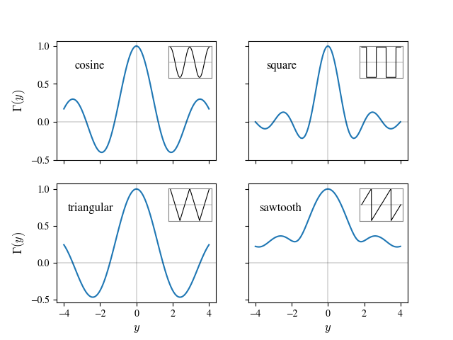
(a)

Figure 1: The matrix element defining the effective interaction between bosons, $\Gamma$, for the various signal shapes, plotted as a function of the variable $y=\kappa g(k_{\ell},k_{m},k_{n},k_{p})$. The analytical expressions for $\Gamma(y)$ are given in Section III. For the sawtooth case, where $\Gamma$ cannot be made real (see discussion in Sections III and IV), we plot $|\Gamma(y)|$.

In this Section we will derive the expression of the effective Hamiltonian (3) for driving functions $f(t)$ other than the cosenoidal signal, but still periodic and with zero time-average over one period. These signals are shown versus time in the insets of Fig. 1. They are taken to have the same period and amplitude.

Equation (3) remains the general effective Hamiltonian, but different profiles of the time signal $f(t)$ now yield different matrix elements of the interaction between plane waves, i.e., different forms of the function $\Gamma(y)$, where $y=\kappa g(k_{\ell},k_{m},k_{n},k_{p})$. We have already seen that for the cosenoidal signal [see Eq. (6)], $\Gamma(y)=\mathcal{J}_{0}(2y)$.

For the square wave signal

$$f(t)=\left\{\begin{array}[]{ll}1,&\omega t\in[0,\pi/2)\\ -1,&\omega t\in[\pi/2,3\pi/2)\\ 1,&\omega t\in[3\pi/2,2\pi)\\ \end{array}\right.,$$ (10)

the matrix element $\Gamma(y)$ (4) takes the form

$$\Gamma(y)=\frac{\sin(\pi y)}{\pi y}\,,$$ (11)

while for the triangular signal

$$f(t)=\frac{2}{\pi}\times\left\{\begin{array}[]{ll}\pi/2-\omega t,&\omega t\in[0,\pi)\\ \omega t-3\pi/2,&\omega t\in[\pi,2\pi)\\ \end{array}\right.,$$ (14)

the expression becomes

$$\Gamma(y)=\frac{\cos\left(\dfrac{\pi y}{2}\right)C(\sqrt{y})+\sin\left(\dfrac{\pi y}{2}\right)S(\sqrt{y})}{\sqrt{y}}\,,$$ (15)

where $C$ and $S$ are the Fresnel cosine and sine integrals Abramowitz and Stegun (1964).

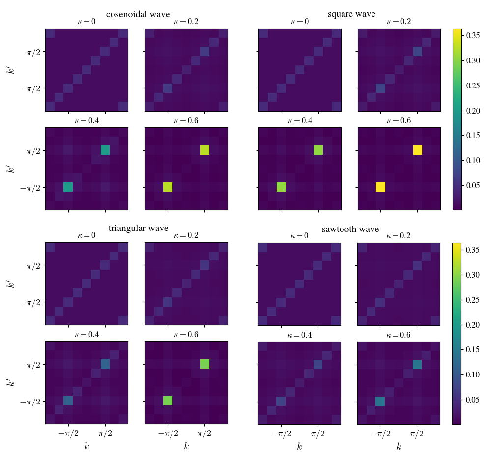
(a)

Figure 2: Two particle momentum density, $\rho^{(2)}(k,k^{\prime})$ as a function of $\kappa$ for each signal shape. For $\kappa=0$ the system is in the Mott state, and $\rho^{(2)}(k,k^{\prime})$ is peaked along the diagonal $k=k^{\prime}$. As $\kappa$ increases, isolated peaks form at $\pm(\pi/2,\pi/2)$, indicating the formation of the superfluid cat-state.

Finally, for the sawtooth signal

$$f(t)=\frac{1}{\pi}\times\left\{\begin{array}[]{ll}\omega t,&\omega t\in[0,\pi)\\ \\ \omega t-2\pi,&\omega t\in[\pi,2\pi)\end{array}\right.,$$ (19)

we obtain

$$\Gamma(y)=\frac{\mathrm{erf}\left(\sqrt{-i\pi y}\right)}{2\sqrt{-iy}},$$ (20)

where $\text{erf}(z)$ is the error function.

Figure 1 shows the plots of $\Gamma(y)$ for the different driving profiles. Since $\Gamma$ is complex for the sawtooth signal, we plot $|\Gamma|$ in that case. For all signals we have $\Gamma(0)=1$.

The non-vanishing of $\Gamma$ for the sawtooth signal can be directly ascribed to its lack of time-reversal symmetry. Unlike the other waveforms we consider, the sawtooth function is not symmetric under the generalized parity operation $(x,t)\rightarrow(-x,t+T/2)$. As a consequence, the quasienergies of $H_{\mathrm{eff}}$ do not have definite parity Großmann and Hänggi (1992), and so the von Neumann-Wigner theorem v. Neumann and Wigner (1929) forbids them making exact crossings as $\kappa$ varies. Instead, they can only form avoided crossings, which in turn implies that the amplitudes for elementary processes, described by $\Gamma(y)$, cannot vanish.

From (3), and using the specific expression of $\Gamma(y)$ of each signal, we calculate the two-particle momentum density

$$\rho^{(2)}(k,k^{\prime})=\frac{1}{N^{2}}\innerproduct{n_{k}n_{k^{\prime}}}{n_{k}n_{k^{\prime}}}.$$ (21)

Results are shown in Fig. 2. All the plots reveal the system is robust against the choice of the driving profile, giving very similar forms for $\rho^{(2)}(k,k^{\prime})$. The only difference is that for the sawtooth, greater values of $\kappa$ are needed to produce peaks with comparable heights to the other cases, which is related to the fact that $\Gamma(y)$ for the sawtooth does not cross the horizontal axis (see Fig. 1).

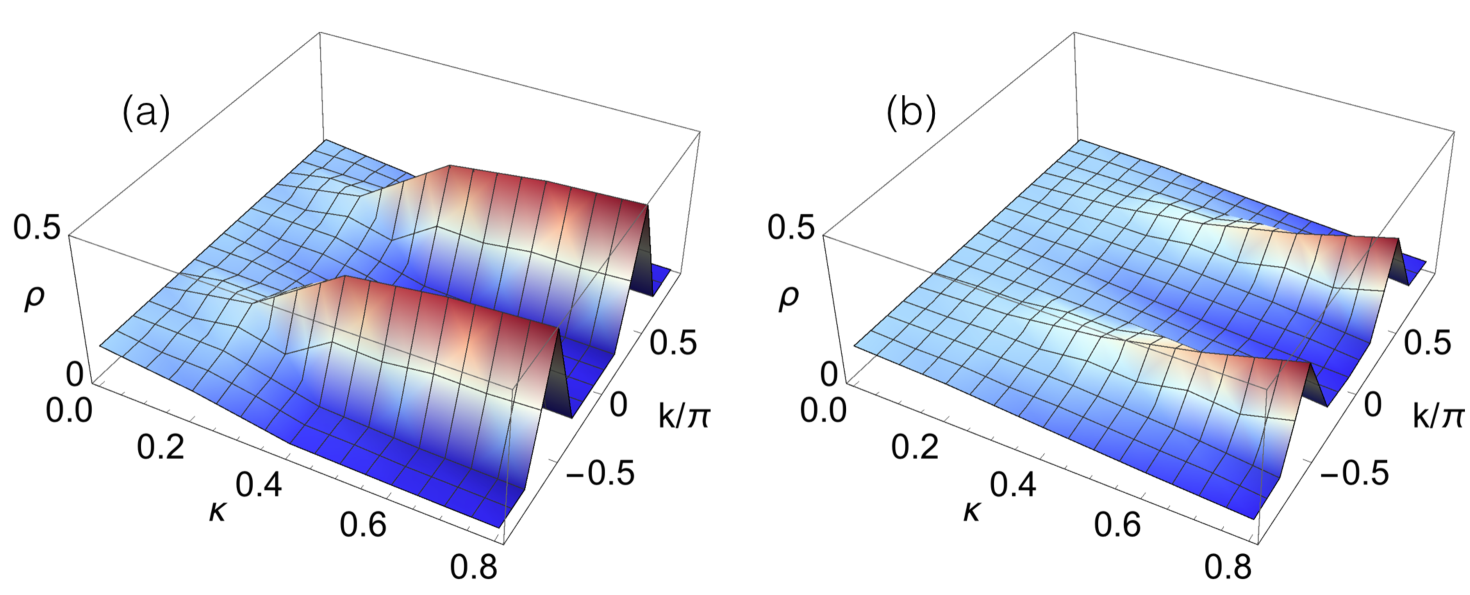
Figure 3: Momentum density, $\rho(k)$, as a function of $\kappa$. (a) Square wave driving. The momentum density is initially flat for $\kappa=0$ when the system is in the Mott state. As $\kappa$ increases the system passes through a phase transition and $\rho(k)$ develops two peaks at $k=\pm\pi/2$, indicating the formation of the superfluid cat state. (b) Sawtooth driving. In contrast to the square wave case, the peaks in $\rho(k)$ develop more slowly, and are much less pronounced.

We now calculate the one-particle momentum density

$$\rho(k)=\frac{1}{N}\innerproduct{n_{k}}{n_{k}}.$$ (22)

for the square and the sawtooth signals, and show the results in Fig. 3. Again, peaks form at $k=\pm\pi/2$ when $\kappa$ grows, indicating the macroscopic occupation of these momentum states as the superfluid state develops. For the sawtooth these peaks in $\rho(k)$ develop more slowly as a function of $\kappa$, showing that larger values of $\kappa$ are required for the system to become superfluid.

In all the cases considered in this Section we have explicitly checked that the full time-dependent evolution under Eq. (1) yields the same results as that obtained from the effective time-independent Hamiltonian $H_{\mathrm{eff}}$. We note that in the numerical simulation of the time evolution, the system is prepared in the Mott state (i.e. the ground state of the zero-hopping Bose-Hubbard Hamiltonian). The kinetic driving is then gradually introduced so that the state evolves adiabatically towards the ground state of the effective time-independent Hamiltonian.

IV Initial phase

It was noted in Refs. Creffield and Sols (2011); Kudo and Monteiro (2011); Kolovsky (2011); Creffield and Sols (2013, 2014), and later observed in cold atoms systems Haller et al. (2010), that if a phase-shift $\varphi$ is added to the standard cosenoidal signal

$$f(t)=\cos(\omega t+\varphi)\,,$$ (23)

then the long-term dynamics can be sensitive to that phase and, in the case of a ring this phase can create the effect of an effective flux threading the ring, enabling the simulation of a synthetic magnetic field. We wish to investigate whether a similar effect appears in the kinetically-driven system. The effective time-independent Hamiltonian becomes Creffield et al. (2016)

$$H_{\mathrm{eff}}=\frac{U}{2L}\sum_{\ell,m,n,p=0}^{L-1}\delta_{k_{\ell}+k_{m},k_{n}+k_{p}} e^{-i2\kappa gF(\varphi)}\Gamma(\kappa g)\ a^{\dagger}_{k_{p}}a^{\dagger}_{k_{n}}a_{k_{m}}a_{k_{\ell}}\,,$$ (24)

where $\Gamma(y)$ is given in the previous Section for the various signal shapes, and the $F$ function reads

$$F(\varphi) =\begin{cases}\sin\varphi\qquad\quad&(\mathrm{cosine\ wave})\\ \varphi&(\mathrm{square\ wave})\\ \varphi-\varphi^{2}/\pi&(\mathrm{triangular\ wave})\\ \varphi^{2}/2\pi&(\mathrm{sawtooth\ wave})\,.\end{cases}$$ (25)

Due to the additive structure of the function $g$ [see Eq. (5)], the presence of $F(\varphi)\neq 0$ amounts to adding a phase to each boson operator

$$a_{k}\rightarrow a_{k}e^{i\alpha_{k}}\,,$$ (26)

where $\alpha_{k}=2\kappa\cos(k)F(\varphi)$. Addition of a global, $k$-dependent phase to each one-particle momentum eigenstate of eigenvalue $k$ does not have any physical consequence, from which we conclude that the system properties are exactly independent of $\varphi$, as can be confirmed numerically.

Thus, unlike the single-particle hopping of independent particles, or in the conventional Bose-Hubbard problem Creffield and Sols (2011, 2013, 2014), it is not possible to create a flux through the ring by tailoring the initial phase of the kinetic driving.

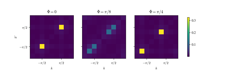
Figure 4: Two-particle momentum density $\rho^{(2)}(k,k^{\prime})$ for several values of $\Phi$, with $\kappa=0.6$. When $\Phi=0$ the peaks are centered on $\pm(\pi/2,\pi/2)$. For $\Phi=\pi/8$ each peak is smeared over two values of momenta, as the momentum shift produced by $\Phi$ is incommensurate with the reciprocal lattice momenta. $\Phi=\pi/4$ is commensurate with the reciprocal lattice and the peaks are shifted by one momentum spacing, $-\pi/4$, along the diagonal.

V Effective flux

An effective external flux $\Phi$ threading the ring may result from a controlled or spurious rotation of the ring. We study here how ground state properties of the system change under the effect of this flux. The fundamental time-dependent Bose-Hubbard Hamiltonian becomes

$$\mathcal{H}(t)=-f(t)\sum_{x=0}^{L-1}\left(e^{i\Phi}a^{\dagger}_{x+1}a_{x}+e^{-i\Phi}a^{\dagger}_{x}a_{x+1}\right)+\frac{U}{2}\sum_{x=0}^{L-1}n_{x}(n_{x}-1),$$ (27)

where we take the cosenoidal driving without any initial phase, $f(t)=\cos(\omega t)$. In this case the effective Hamiltonian becomes

$$H_{\mathrm{eff}}(\Phi)=\frac{U}{2L}\sum_{\ell,m,n,p=0}^{L-1}\delta_{k_{\ell}+k_{m},k_{n}+k_{p}}\mathcal{J}_{0}\left[2\kappa g(k_{\ell},k_{m},k_{n},k_{p};\Phi)\right]a^{\dagger}_{k_{p}}a^{\dagger}_{k_{n}}a_{k_{m}}a_{k_{\ell}}$$ (28)

where the $g$-function is now defined by

$$g(k_{\ell},k_{m},k_{n},k_{p};\Phi)=\cos(k_{\ell}+\Phi)+\cos(k_{m}+\Phi)-\cos(k_{n}+\Phi)-\cos(k_{p}+\Phi).$$ (29)

This is the main difference between this case and the previous one; $\Phi$ does not appear as a phase factor, but inside the arguments of the cosine functions. Accordingly $\Phi$ does have a physically observable effect, shifting the momentum at which the peaks of $\rho^{(2)}(k,k^{\prime})$ occur. In Fig. 4 (left) we shown the two-particle momentum density for $\Phi=0$, which displays narrow peaks centered on $\pm(\pi/2,\pi/2)$. When a phase of $\Phi=\pi/8$ is introduced, Eq. (29) predicts these peaks should be shifted in momentum space by $\Delta k=\pi/8$. However, for the 8-site ring we consider, this shift is not commensurate with the reciprocal lattice momenta, and so the peaks spread over the two closest momenta to the shifted values, as shown in Fig. 4 (center). The smallest non-zero shift of momentum that is commensurate with the lattice is $\Delta k=2\pi/8=\pi/4$. For $\Phi=\pi/4$, the peaks are indeed shifted by this quantity, so they now are located at $(-3\pi/4,-3\pi/4)$ and $(\pi/4,\pi/4)$, as can be seen in Fig. 4 (right).

The fact that for $\Phi=\pi/8$ we find a preferential occupation of the available momenta which are closest to the ideal one reflects the physical continuity of the occupation as a function of momentum, which is somewhat obscured in this model with just a few momentum states. In the thermodynamic limit we can expect to find a smoothly enhanced occupation of momenta near $\pm\pi/2$, and a hint of this behavior can already be observed in Fig. 3, where an enhancement of the occupation is already observed in momenta near $\pm\pi/2$.

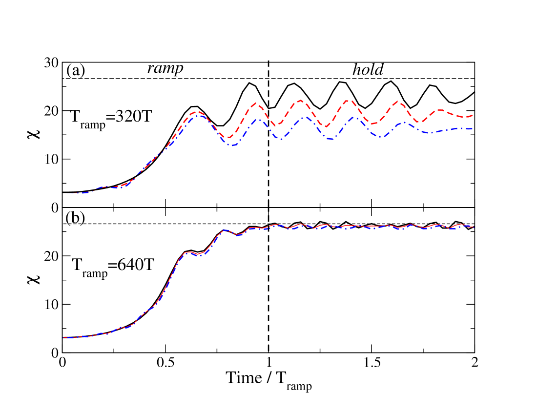
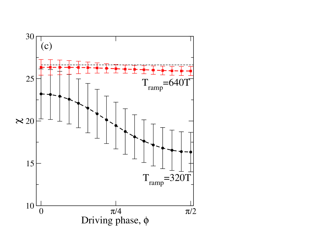
Figure 5: Fidelity of the ramp protocol in preparing the cat state at $\kappa=0.8$, as measured by $\chi$. (a) For a ramp-time of $T_{\mathrm{ramp}}=320T$ the fidelity of the final state depends strongly on the phase of the driving. Cosinusoidal driving (black solid line) shows the best performance, and sinusoidal driving (blue dot-dashed line) the worst. An intermediate phase, $f(t)=\cos(\omega t-\pi/4)$ (red dashed line) lies between these results. The value of $\chi$ in the true ground state of the system is shown by the horizontal dashed line. (b) When the ramp-time is increased to to $T_{\mathrm{ramp}}=640T$ the driving phase barely affects the result. (c) Dependence of $\chi$ on the phase of the driving for the two ramp-times. Error bars indicate the amplitude of the oscillations of the final state. Physical parameters: $U=1$, $\omega=50$.

VI Adiabatic state preparation

We now consider the feasibility of preparing the cat state in experiment, using the technique of adiabatic manipulation. We initialise the system in the Mott state, with one particle occupying each site of the lattice, and then gradually increase the value of $\kappa$ from zero to $\kappa=0.8$. If this increase is done sufficiently slowly, so that the system remains in its ground-state at all times, the Mott-state will be adiabatically transformed into the exotic superfluid state. In particular we consider the protocol in which the amplitude of $\kappa$ is ramped up linearly over a long time-interval $T_{\mathrm{ramp}}$, which may be many hundred of driving periods long, and then held at a constant value for a period we term the “hold-time”. To quantify the quality of the state preparation, we measure the quantity $\chi=\langle n_{\pi/2}n_{\pi/2}\rangle$, that is, the $\left(\pi/2,\pi/2\right)$ component of the two-particle reduced density matrix. This quantity takes a high value in the cat state, and so acts as a good figure of merit Pieplow, Creffield, and Sols (2019) to identify a state’s “cattiness”.

In Fig. 5a we show the result for sinusoidal driving, $f(t)=\cos\left(\omega t+\varphi\right)$, for three different values of the driving phase $\varphi$, using a ramp-time of $T_{\mathrm{ramp}}=320T$. When the driving is cosinusoidal ($\varphi=0$), the value of $\chi$ initially rises smoothly, but then begins to oscillate towards the end of the ramp, and these oscillations continue during the hold-time. This arises from the form of the quasienergy spectrum of the system. When the system is in the Mott state, the spectrum is gapped and the ground-state is well-separated from the higher energy states. Consequently the adiabatic condition is easily satisfied and the system smoothly tracks the instantaneous ground-state as $\kappa$ increases. As the system passes through the phase transition to the superfluid state, however, this gap closes, and unless the ramp speed is extremely slow some proportion of the state will be excited out of the instantaneous ground state, producing the oscillatory behaviour. Changing the driving-phase to $\varphi=\pi/4$ produces a qualitatively similar behaviour, but the maximum value of $\chi$ is smaller, indicating that the final state has been prepared with less fidelity. For a sinusoidal driving ($\varphi=\pi/2$) the fidelity is reduced even further.

The $\varphi$-dependence of these results may appear surprising, since in Section IV it was shown that the driving-phase had no effect on the system. However, that lack of $\varphi$-dependence only applies strictly to the ramping procedure in the adiabatic limit, $T_{\mathrm{ramp}}\rightarrow\infty$. In Fig. 5b we show the effect of doubling the ramp-time to $T_{\mathrm{ramp}}=640T$. With this slower ramp, the procedure is more adiabatic, and indeed the $\varphi$-dependence of the results is considerably reduced. As a consequence the maximum value of $\chi$ following the ramp is much closer to the value for the $\kappa=0.8$ superfluid ground state, and the oscillations in $\chi$ are much reduced. We quantify this further in Fig. 5c, showing the $\varphi$ dependence of $\chi$ for the slow and the fast ramp-times. Clearly as $T_{\mathrm{ramp}}$ increases, the $\varphi$ dependence of the results decreases, and the fidelity of the process improves. From this graph it is also clear that if an experiment is limited to low or moderate values of the ramp-time, the best choice of the driving will be cosenoidal.

VII Conclusions

We have investigated the sensitivity of a many-boson system to the details of the kinetic driving previously explored in Pieplow, Sols, and Creffield (2018); Pieplow, Creffield, and Sols (2019), where the hopping energy oscillates periodically in time with zero average. In particular we have studied the sensitivity of the cat-like structure of the ground state to the shape of the signal profile, phase-shifts of the driving, and the presence of an external magnetic flux. We have found that the system is very sensitive to the symmetry of the time signal. The sawtooth profile exemplifies the case where time-reversal symmetry is absent, and the cat-like properties of the ground state are considerably diminished. The fact that the interaction matrix elements between plane waves cannot vanish makes them weakly dependent on the strength of the driving, thus favoring less markedly the collision processes that in Pieplow, Creffield, and Sols (2019) were shown to underlie the ground-state cat structure.

In contrast to the case of the standard driven Bose-Hubbard model, we find that introducing a phase-shift to the driving signal does not affect the properties of the system at all. Instead of producing hopping phases, as might be expected, the system is completely blind to this form of perturbation. Introducing hopping phases by rotating the ring to produce an effective flux, only has the effect of trivially displacing the momenta at which the quasi-condensates form. In particular, the cat structure of the ground state remains intact.

We have also explored the preparation of the cat-state in experiment, by adiabatically ramping the driving from zero. In the deep adiabatic limit, the process becomes insensitive to the phase of the driving, while a cosenoidal signal gives the optimum fidelity for shorter ramp-times.

In conclusion, the main properties of the kinetically driven superfluid boson system are rather robust against variations in the details of the driving, provided that the signal is time symmetric. In addition, we have shown that suitably choosing the phase of the driving allows the adiabatic preparation to be substantially shortened.

References

- Oka and Kitamura (2019) T. Oka and S. Kitamura, Annual Review of Condensed Matter Physics 10, 387 (2019).
- Eckardt, Weiss, and Holthaus (2005) A. Eckardt, C. Weiss, and M. Holthaus, Phys. Rev. Lett. 95, 260404 (2005).
- Creffield and Monteiro (2006) C. E. Creffield and T. S. Monteiro, Phys. Rev. Lett. 96, 210403 (2006).
- Rapp, Deng, and Santos (2012) A. Rapp, X. Deng, and L. Santos, Phys. Rev. Lett. 109, 203005 (2012).
- Liberto et al. (2014) M. D. Liberto, C. E. Creffield, G. I. Japaridze, and C. M. Smith, Phys. Rev. A 89, 013624 (2014).
- Pieplow, Sols, and Creffield (2018) G. Pieplow, F. Sols, and C. E. Creffield, New Journal of Physics 20, 073045 (2018).
- Stöferle et al. (2004) T. Stöferle, H. Moritz, C. Schori, M. Köhl, and T. Esslinger, Phys. Rev. Lett. 92, 130403 (2004).
- Kollath et al. (2006) C. Kollath, A. Iucci, T. Giamarchi, W. Hofstetter, and U. Schollwöck, Phys. Rev. Lett. 97, 050402 (2006).
- Sensarma et al. (2009) R. Sensarma, D. Pekker, M. D. Lukin, and E. Demler, Phys. Rev. Lett. 103, 035303 (2009).
- Citro et al. (2020) R. Citro, E. Demler, T. Giamarchi, M. Knap, and E. Orignac, arXiv:2003.05373 (2020).
- Pieplow, Creffield, and Sols (2019) G. Pieplow, C. E. Creffield, and F. Sols, Phys. Rev. Research 1, 033013 (2019).
- Abramowitz and Stegun (1964) M. Abramowitz and I. A. Stegun, Handbook of Mathematical Functions with Formulas, Graphs, and Mathematical Tables (Dover, New York, 1964).
- Großmann and Hänggi (1992) F. Großmann and P. Hänggi, Europhysics Letters (EPL) 18, 571 (1992).
- v. Neumann and Wigner (1929) J. v. Neumann and E. Wigner, Phys. Z. 30, 467 (1929).
- Creffield and Sols (2011) C. E. Creffield and F. Sols, Phys. Rev. A 84, 023630 (2011).
- Kudo and Monteiro (2011) K. Kudo and T. S. Monteiro, Phys. Rev. A 83, 053627 (2011).
- Kolovsky (2011) A. R. Kolovsky, EPL (Europhysics Letters) 93, 20003 (2011).
- Creffield and Sols (2013) C. E. Creffield and F. Sols, EPL (Europhysics Letters) 101, 40001 (2013).
- Creffield and Sols (2014) C. E. Creffield and F. Sols, Phys. Rev. A 90, 023636 (2014).
- Haller et al. (2010) E. Haller, R. Hart, M. J. Mark, J. G. Danzl, L. Reichsöllner, and H.-C. Nägerl, Phys. Rev. Lett. 104, 200403 (2010).
- Creffield et al. (2016) C. E. Creffield, G. Pieplow, F. Sols, and N. Goldman, New Journal of Physics 18, 093013 (2016).