Laser-nucleus interactions in the sudden regime

Abstract

The interaction between medium-weight nuclei and a strong zeptosecond laser pulse of MeV photons is investigated theoretically. Multiple absorption of photons competes with nuclear equilibration. We investigate the sudden regime. Here the rate of photon absorption is so strong that there is no time for the nucleus to fully equilibrate after each photon absorption process. We follow the temporal evolution of the system in terms of a set of rate equations. These account for dipole absorption and induced dipole emission, equilibration (modeled in terms of particle-hole states coupled by the residual nuclear interaction), and neutron decay (populating a chain of proton-rich nuclei). Our results are compared with earlier work addressing the adiabatic regime where equilibration is instantaneous. We predict the degree of excitation and the range of nuclei reached by neutron evaporation. These findings are relevant for planning future experiments.

I Introduction

Exciting experimental developments at petawatt laser facilities Danson et al. (2019) combined with experimental, computational and theoretical advances in the production of high-energy laser pulses Esirkepov, T. Zh. et al. (2009); Kiefer, D. et al. (2009); Meyer-ter-Vehn, J. and Wu, H.-C. (2009); Mourou and Tajima (2011); Kiefer et al. (2013); Bulanov et al. (2013); Mu et al. (2013); Li et al. (2014) give rise to the hope that intense pulses with photon energy $\hbar\omega_{0}$ in the few MeV range and with a typical energy spread $\sigma$ in the $10$ keV range will become available in the near future. Efforts in that direction are presently undertaken at the Nuclear Pillar of the Extreme Light Infrastructure under construction in Romania Extreme Light Infrastructure Nuclear Physics (2019) (ELI-NP), and in the development of Gamma Factories at the Large Hadron Collider of CERN Płaczek et al. (2019). How would such a pulse interact with a nucleus?

For a photon with an energy in the MeV range, the product of photon wave number $k$ and nuclear radius $R$ obeys $kR\ll 1$. Therefore, we consider only dipole processes (even though higher multipolarities might be important for some nuclei at small excitation energies Pálffy et al. (2008)). Single dipole absorption excites the nuclear giant dipole resonance (GDR). In a shell-model picture the GDR is a superposition of particle-hole excitations out of the ground state and is not an eigenstate of the nuclear Hamiltonian $\hat{H}$. These particle-hole excitations actually do not all have the same energy. That leads to a spreading of the GDR often referred to as Landau damping, a one-body effect Fiolhais (1986); Speth and Wambach (1991). The residual two-body interaction mixes the particle-hole excitations with each other and with other shell-model configurations and, thus, spreads the GDR over the eigenstates of $\hat{H}$, leading to a Lorentzian distribution of the dipole strength with width $\Gamma^{\downarrow}$. For low-lying modes with excitation energies of up to 10 or 20 MeV the “spreading width” $\Gamma^{\downarrow}$ of the nuclear GDR Feshbach (1964); Herman et al. (1992) has values around $5$ MeV Weidenmüller and Mitchell (2009). In a time-dependent picture the spreading of the GDR over the eigenstates of $\hat{H}$ can be viewed as statistical equilibration Agassi et al. (1975) with characteristic time scale $\tau_{\rm eq}=\hbar/\Gamma^{\downarrow}$. A similar order of magnitude for the generic time required to reach thermal equilibrium $\tau_{\rm eq}\simeq 10^{-22}$ s can be achieved by considering the traversal time for medium-weight nuclei Bortignon et al. (1991). We note however that the definition of an equilibration time becomes more complex once very high excitation energies are achieved, for instance in hot GDRs Santonocito and Blumenfeld (2020), accompanied by strong neutron evaporation rates and corresponding short lifetimes Bortignon et al. (1991).

The strength of dipole absorption is measured by the rate $R_{\rm dip}$ (or, equivalently, by the effective dipole width $\widetilde{\Gamma}_{\rm dip}=\hbar R_{\rm dip}$ or the time scale $\tau_{\rm dip}=\hbar/\widetilde{\Gamma}_{\rm dip}$ for dipole absorption). The standard nuclear dipole width has values in the keV range. However, for a laser pulse containing $N\gg 1$ photons within few tens of zs (1 zs$=10^{-21}$ s), that width is boosted by the factor $N$ even when the pulse is not coherent Pálffy et al. (2020), and the effective dipole width can easily take values in the MeV range. That makes multiple dipole absorption of photons out of the same laser pulse a likely process.

For the following qualitative comparison of $\widetilde{\Gamma}_{\rm dip}$ and $\Gamma^{\downarrow}$ we consider both quantities as independent of excitation energy. That picture is only an approximation. Experimental evidence for hot GDR quenching Santonocito and Blumenfeld (2020) was interpreted as an increase of $\Gamma^{\downarrow}$ with temperature, reaching up to 20 MeV (50 MeV) at 160 MeV (220 MeV) excitation energy, respectively Yoshida et al. (1990). Such an increase of $\Gamma^{\downarrow}$ with temperature would lead to a weak decrease of the effective dipole absorption width $\widetilde{\Gamma}_{\rm dip}$ as indicated by the expression for $R_{\rm dip}$ Pálffy et al. (2020). However, for the mere purpose of defining laser-nucleus interaction regimes, it is sufficient to compare the two widths at small excitation energies, where they can reach comparable values depending on the laser gamma-ray parameters. Once $\widetilde{\Gamma}_{\rm dip}\approx\Gamma^{\downarrow}$, we expect that multiple dipole absorption leads to multiple GDR-type excitations, each accompanied by internal nuclear equilibration. The ratio of the two competing widths $\Gamma^{\downarrow}$ and $\widetilde{\Gamma}_{\rm dip}$ then defines three regimes: (i) the perturbative regime $\widetilde{\Gamma}_{\rm dip}\ll\Gamma^{\downarrow}$, (ii) the quasiadiabatic regime $\widetilde{\Gamma}_{\rm dip}\leq\Gamma^{\downarrow}$ and (iii) the sudden regime $\widetilde{\Gamma}_{\rm dip}\gg\Gamma^{\downarrow}$. The perturbative regime (i) was studied in Refs. Dietz and Weidenmüller (2010); Weidenmüller (2011). The term “quasiadiabatic” in (ii) refers to the assumption that after each photon absorption process, the nucleus reaches equilibrium prior to the absorption of the next photon. Theoretical and numerical studies Pálffy and Weidenmüller (2014); Pálffy et al. (2015) in that regime are based on a statistical approach and make use of rate equations. These have shown that multiple photon absorption produces compound nuclei in the so-far unexplored regime of several hundred MeV excitation energy and low angular momentum. The nuclei so produced undergo sequential neutron decay with intermittent further dipole absorption and equilibration, leading to a chain of highly excited proton-rich nuclei.

In this paper we address the sudden regime (iii). To model a situation where after each photoabsorption process there is not sufficient time for equilibration, we need a detailed description of the states of the compound nucleus. We use the shell model, assuming that the ground state of the target nucleus has a doubly-closed shell. The last occupied single-particle state defines the Fermi surface. Excited states are multiple particle-hole excitations out of the ground state (referred to as $m$p-$m$h states with integer $m$).

For that picture, a manageable theoretical framework cannot be established without statistical assumptions. Particle-hole states are grouped into classes defined by particle-hole number $m$ and total energy, as discussed in more detail in Sec. II.1. It is assumed that within each class of $m$p-$m$h states, the residual interaction is so strong that equilibration is much faster than the equilibration between different classes, and can be considered to be quasi instantaneous. This assumption is also used in precompound reaction models and has proven its validity by good agreement with experimental data Blann (1975). A second related assumption is that because of the strong mixing within one class, the eigenfunctions of the time-independent Hamiltonian are Gaussian-distributed random variables, and the eigenvalues obey Wigner-Dyson statistics Weidenmüller (2021). This assumption was thoroughly tested in Ref. Zelevinsky et al. (1996). These two assumptions guarantee that both the matrix elements of the residual interaction connecting states in different classes and those of the dipole operator, are zero-centered Gaussian-distributed random variables Agassi et al. (1975). Rates are obtained as mean values over these distributions. The rates for nuclear equilibration are proportional to mean values of squares of matrix elements of the residual interaction connecting states in different classes, and to the level density of the $m$p-$m$h states reached. The rate for dipole absorption is similarly proportional to the mean square matrix element for dipole absorption Pálffy et al. (2020) and to the density of final states. Multiple dipole absorption leads to nuclear excitation far above yrast. Calculation of the rates requires, therefore, the knowledge of $m$p-$m$h level densities at high excitation energy (up to several $100$ MeV) and for large particle numbers. A reliable approximation for these densities in terms of the single-particle level density of the shell model was worked out in Refs. Pálffy and Weidenmüller (2013a, b) and is used in what follows.

The rates are used in rate equations. These describe the time evolution of the average occupation probabilities of classes of $m$p-$m$h states under the influence of the external field of the laser. They account for the following competing processes: photoabsorption and its inverse process stimulated photon emission, equilibration, and neutron evaporation. In a manner similar to the theory of precompound reactions Weidenmüller (2008), equilibration is taken into account by coupling different $m$p-$m$h classes at the same energy. Absorption of a photon by an $m$p-$m$h state either generates an additional particle-hole pair promoting the nucleus to class $(m+1)$p-$(m+1)$h, or it increases the energy of an existing particle-hole pair. Conversely, stimulated emission leads to the annihilation of a particle-hole pair, or it reduces the energy of an existing particle-hole pair without changing $m$. We disregard here possible collective excitations which could play a role at small excitation energies. Neutron evaporation changes mass number from even to odd and conversely. For odd-mass nuclei we interpolate between the neighboring even-mass nuclei. We consider, thus, only states with equal particle-hole numbers. We neglect particle loss from direct photon excitation of particles (protons or neutrons) into continuum states. Thus we confine ourselves to a chain of nuclei with equal proton numbers. Ensuing limitations and possible corrections have been addressed qualitatively in Ref. Pálffy et al. (2015) for the quasiadiabatic regime. The relevance of these processes for the deep sudden regime is briefly addressed in the concluding remarks of this paper in Sec. IV. We simplify the treatment of the problem by disregarding spin altogether. That was justified in Ref. Pálffy et al. (2015) by the slow increase of total spin value with multiple photon absorption.

We consider the interaction of a strong zeptosecond laser pulse with a medium-weight nucleus with mass number $A$. For $\widetilde{\Gamma}_{\rm dip}$ we use values in the range $1$ – $20$ MeV. In the course of the reaction, up to $N_{0}\approx 140$ photons may be absorbed. We neglect the resulting reduction of $N\to N-N_{0}$ in the boost factor of $\widetilde{\Gamma}_{\rm dip}$. The energy $\hbar\omega_{0}$ per photon is $5$ MeV, and the duration of the pulse is $\tau=\hbar/\sigma$ where $\sigma$ is of the order of several $10$ keV so that $\tau\approx 10^{-20}$ s. We investigate the temporal evolution of the nucleus over the laser pulse duration, and we follow the chain of neutron evaporation processes towards proton-rich nuclei. Fission is expected to be important only for very heavy nuclei and is disregarded. To illustrate the role of the equilibration process, we compare results for the sudden and for the quasiadiabatic regime. In the absence of nucleon emission and fission, photon absorption would saturate at an excitation energy where the rates for absorption and for stimulated emission become equal. That energy is given by the maximum of the total level density summed over all particle-hole classes. The larger the effective dipole absorption rate, the faster this saturation energy is reached. Neutron evaporation takes over at an energy below the saturation point. The combination of repeated neutron emission and continued dipole absorption by the daughter nuclei then produces proton-rich nuclei far from the valley of stability. This picture is qualitatively similar to but quantitatively somewhat different from the results for the quasiadiabatic regime.

The paper is structured as follows. The rate equation and the transition rates are introduced in Sec. II. This section also addresses the densities of accessible states for $m$p-$m$h classes. Numerical results follow in Sec. III and the paper concludes with a discussion in Sec. IV.

II Rate Equations

II.1 Basic Approach

With $A$ the even mass number of the target nucleus, we consider a chain of $(n+1)$ nuclei with mass numbers $A-i$ where $i=0,1,2,\ldots,n$, with an arbitrary cutoff at $i=n$. In the target ($i=0$), absorption of $k$ laser photons will increase the excitation energy by $k\hbar\omega_{0}$ and potentially also change the particle-hole number. We group the nuclear states according to the generation $i$, the particle-hole number $m$, and the total energy, which for our case will be a multiple of the laser photon energy $\hbar\omega_{0}$. In the following we therefore use classes labeled $(i,k,m)$. The equilibration processes between classes are discussed below. The level density in each class is $\rho_{m}(0,k)$. Single or multiple neutron decay of the target populates an energy continuum of states in the daughter nuclei labeled $i=1,2,\ldots,n$. For even-mass daughter nuclei $i$, the $m$p-$m$h states in the energy interval between $(k-1/2)\hbar\omega_{0}$ and $(k+1/2)\hbar\omega_{0}$ form class $(i,k,m)$. The class of particle-hole states with excitation energies in the interval $0\leq E\leq(1/2)\hbar\omega_{0}$ is labeled $(i,0,m)$. The average level density of the states in class $(i,k,m)$ is denoted by $\rho_{m}(i,k)$. For odd-mass daughter nuclei we use energy intervals $k$ defined in the same manner. We avoid introducing $m$p-$(m\pm 1)$h states and their level densities and use a simplification instead. We neglect the even-odd staggering of the ground-state energies as well as that of the spin-cutoff factor, and we approximate the level density for odd $i$ by interpolating between the values for the two neighboring even-mass nuclei. In other words, we use the expression for the level density for even mass numbers given in Ref. Pálffy and Weidenmüller (2013b) indiscriminately for both even and odd $A$.

The rate equation for the average total occupation probability $P_{m}(i,k,t)$ of the states in class $(i,k,m)$ as a function of time $t$ is

$$\dot{P}_{m}(i,k,t) = \sum_{m^{\prime}=m\pm 1}V^{2}_{m^{\prime}m}(i,k)\rho_{m}(i,k)P_{m^{\prime}}(i,k,t)-\sum_{m^{\prime}=m\pm 1}V^{2}_{mm^{\prime}}(i,k)\rho_{m^{\prime}}(i,k)P_{m}(i,k,t)$$ (1)

$$+ \Theta(\tau-t)\sum_{m^{\prime}=m,m\pm 1}\bigg{\{}W^{2}_{k-1k;m^{\prime}m}(i)\rho_{m}(i,k)P_{m^{\prime}}(i,k-1,t)+W^{2}_{k+1k;m^{\prime}m}(i)\rho_{m}(i,k)P_{m^{\prime}}(i,k+1,t)$$

$$- W^{2}_{kk+1;mm^{\prime}}(i)\rho_{m^{\prime}}(i,k+1)P_{m}(i,k,t)-W^{2}_{kk-1;mm^{\prime}}(i)\rho_{m^{\prime}}(i,k-1)P_{m}(i,k,t)\bigg{\}}$$

$$- \Gamma_{\rm N}(i,k,m)P_{m}(i,k,t)+\sum_{\begin{subarray}{c}k^{\prime}\\ m^{\prime}=m,m+1\end{subarray}}\Gamma_{\rm N}(i-1,k^{\prime}\to k,m^{\prime}\to m)P_{m^{\prime}}(i-1,k^{\prime},t)\ .$$

We have put $\hbar=1$. The dot denotes the time derivative. The equation takes into account three processes: (i) equilibration of occupation probability of the different $m$p-$m$h classes at constant energy (first line); (ii) dipole excitation and stimulated dipole emission by the MeV laser pulse (second and third line); and (iii) neutron evaporation populating nucleus $A-i-1$ at the expense of nucleus $A-i$ (last line, where we have defined $P_{m}(-1,k,t)=0$). The Heaviside function $\Theta$ accounts for the fact that process (ii) occurs only for the duration time $\tau$ of the laser pulse. The initial condition is $P_{m}(i,k,0)=\delta_{i0}\delta_{k0}\delta_{m0}$.

In each nucleus $i$, the equilibration process (i) involves the coupling of classes $(i,k,m)$ at fixed energy $k\hbar\omega_{0}$ by the residual interaction. The rate is given by $V_{m^{\prime}m}^{2}\rho_{m}(i,k)$, with $V^{2}_{mm^{\prime}}=V^{2}_{m^{\prime}m}$ the mean square matrix element. We recall here our basic picture: Dipole absorption primarily populates distinct particle-hole states with somewhat different energies (Landau damping) Fiolhais (1986); Speth and Wambach (1991). We assume that the states within the same $m$p-$m$h class are quickly mixed by the residual two-body interaction. The remaining part of the residual two-body interaction mixes classes of states with different $m$ with rate $V_{m^{\prime}m}^{2}\rho_{m}(i,k)$. Obviously only neighboring classes $m^{\prime}=m\pm 1$ (see Fig. 1) are coupled. The inverse of the total time needed for such mixing equals $\Gamma^{\downarrow}/\hbar$. That picture is supported by the temperature dependence of the hot GDR width which is interpreted as being from two-body collisions Smerzi et al. (1991); Santonocito and Blumenfeld (2020). Class $(i,k,m)$ may gain (lose) occupation probability because of feeding from (depletion to) classes $(i,k,m\pm 1)$, respectively. Equilibrium is reached when $P_{m}(i,k,t)\propto c\rho_{m}(i,k)$ with a constant $c$ independent of $m$.

For processes (ii), the class $(i,k,m)$ is fed by coherent dipole excitation of classes $(i,k-1,m)$ and $(i,k-1,m-1)$ and by stimulated dipole emission from classes $(i,k+1,m+1)$ and $(i,k+1,m)$. Class $(i,k,m)$ is depleted by dipole absorption exciting classes $(i,k+1,m)$ and $(i,k+1,m+1)$, and by stimulated dipole emission to classes $(i,k-1,m)$ and $(i,k-1,m-1)$. Processes where dipole transitions change (do not change) particle-hole number are illustrated in Fig. 2 (in Fig. 3, respectively). The rates feeding class $(i,k,m)$ are written as $W_{k^{\prime}k;m^{\prime}m}^{2}(i)\rho_{m}(i,k)$ with $k^{\prime}=k-1,\,m^{\prime}=m,m-1$ and $k^{\prime}=k+1,\,m^{\prime}=m,m+1$. Here $W^{2}_{kk^{\prime};mm^{\prime}}(i)=W^{2}_{k^{\prime}k;m^{\prime}m}(i)$ is the average square of the transition matrix element. We have simplified the notation by summing $m^{\prime}$ indiscriminately over $m$ and $m\pm 1$. That requires that we set $W_{k-1k;m+1m}^{2}(i)=0=W_{k+1k;m-1m}^{2}(i)$.

The neutron decay process (iii) depletes the states in class $(i,k,m)$ at the rate $\Gamma_{N}(i,k,m)$. Neutron decay of the states $(i-1,k^{\prime},m^{\prime})$ in the parent nucleus with mass number $A+1-i$ feeds the states in class $(i,k,m)$ with the rate $\Gamma_{N}(i-1,k^{\prime}\to k,m^{\prime}\to m)$. We allow only for $m=m^{\prime},m^{\prime}-1$.

The set of rate equations (1) is similar in spirit to but much more involved than the master equation solved in the quasiadiabatic case Pálffy and Weidenmüller (2014); Pálffy et al. (2015). There, equilibration was assumed from the outset. At fixed excitation energy only the total occupation probability and the total level density (both summed over all $m$) come into play. There are no particle-hole classes. In our case, separate treatment of the particle-hole classes obviously increases the number of coupled differential equations significantly.

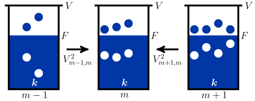
Figure 1: Transitions into class $m$ from neighboring classes ${m\pm 1}$ described by the nucleon-nucleon interaction matrix element $V_{m^{\prime}m}(i,k)$. Here $F$ represents the Fermi energy and $V$ the threshold energy of the single-particle potential. Particles (blue filled circles) are above $F$; holes (white full circles) are below $F$.

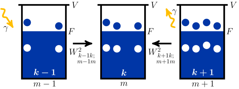
Figure 2: Transitions into class $(i,k,m)$ from neighboring classes $(i,k-1,m-1)$ and $(i,k+1,m+1)$ owing to the laser-nucleus interaction matrix element $W_{k^{\prime}k;m^{\prime}m}(i)$ with $m^{\prime}=m\pm 1$. See Fig. 1 for further notation.

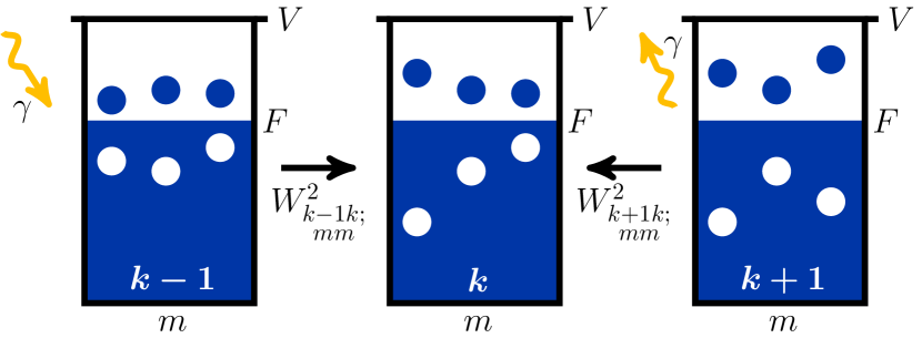
Figure 3: Transitions into class $(i,k,m)$ from neighboring classes $(i,k-1,m)$ and $(i,k+1,m)$ owing to the laser-nucleus interaction matrix element $W_{k^{\prime}k;mm}(i)$. See Fig. 1 for further notation.

II.2 Transition Rates

In this section we give expressions for the rates of the three processes. We mention in passing that for the adiabatic case the rates for processes (ii) and (iii) have been defined, calculated, and discussed in Refs. Pálffy and Weidenmüller (2014); Pálffy et al. (2015). Because $\hbar=1$ we use the expressions “width” and “rate” interchangeably.

II.2.1 Equilibration rate

Equilibration is the result of the coupling of neighboring particle-hole classes at constant energy. To estimate that coupling we use the optical model (see Ref. Herman et al. (1992)). The imaginary part $W(\varepsilon)$ of the optical model potential for nucleons accounts for two-body collisions that remove a nucleon at energy $\varepsilon$ above the Fermi energy from the incident channel and create a $2$p-$1$h state. As function of time, the occupation probability in the incident channel decreases exponentially as $\exp\{-2W(\varepsilon)t\}$. Therefore, we identify $2W(\varepsilon)$ with the spreading width of a (quasiparticle) nucleon above the Fermi surface. The concept of the optical model applies also to hole states, with $\varepsilon$ now the energy of the hole, i.e., the energy below the Fermi energy. Each particle and each hole in an $m$p-$m$h state at energy $E$ may undergo a two-body collision leading to an $(m+1)$p-$(m+1)$h state. The total spreading width for such a particle (hole) is obtained by averaging the optical model over the normalized probability $D_{\mathrm{p}}(m,\varepsilon,E)$ for finding the particle (hole) at energy $\varepsilon$ in the $m$p-$m$h state at energy $E$. The total spreading width for all $m$ particles (holes) is obtained by multiplying the result by $m$. Thus,

$$\Gamma_{m\to m+1}^{\downarrow} = 2m\int\limits_{0}^{V-F}D_{\mathrm{p}}(m,\varepsilon,E)W(\varepsilon)d\varepsilon$$ (2)

$$+ 2m\int\limits_{0}^{F}D_{\mathrm{h}}(m,\varepsilon,E)W(\varepsilon)d\varepsilon\ .$$

We recall that $V$ is the threshold energy of the shell-model potential and $F$ the Fermi energy, respectively. The distributions are given by Herman et al. (1992)

$$\begin{array}[]{l}{D_{\mathrm{p}}(m,\varepsilon,E)=K_{\mathrm{p}}\dfrac{\tilde{\rho}_{m-1,m}(i,E-\varepsilon)}{\rho_{m}(i,E)}}\ ,\\ {D_{\mathrm{h}}(m,\varepsilon,E)=K_{\mathrm{h}}\dfrac{\tilde{\rho}_{m,m-1}(i,E-\varepsilon)}{\rho_{m}(i,E)}}\ .\end{array}$$ (3)

Here $K_{\mathrm{p}}$ and $K_{\mathrm{h}}$ are normalization constants, and $\tilde{\rho}_{p,h}(i,E)$ with $p\neq h$ is the density of $p$p-$h$h states at energy $E$. Finally we use

$$\Gamma_{m\to m+1}^{\downarrow}=2\pi{V_{mm+1}^{2}}(i,k)\rho_{m+1}(i,k)\ .$$ (4)

For the process $m\to(m-1)$ we use $V^{2}_{mm^{\prime}}=V^{2}_{m^{\prime}m}$ and detailed balance so that

$$\Gamma_{m\to m-1}^{\downarrow}=\Gamma_{m-1\to m}^{\downarrow}\frac{\rho_{m-1}(i,k)}{\rho_{m}(i,k)}\ .$$ (5)

Following Refs. Mahaux et al. (1985); Herman et al. (1992), we use $W(\varepsilon)=c\varepsilon^{2}$, with $c=0.003$ MeV^-1. Further employing Eqs. (2) – (5), and the level densities given in Sec. II.2.4 below, we arrive at the numerical values for the rates used in Eqs. (1).

II.2.2 Dipole transitions

The effective dipole width for excitation starting from the ground state is given by $\widetilde{\Gamma}_{\rm dip}$. Among others, it depends on the total number of photons in and on the aperture of the pulse Pálffy et al. (2020), both experimental parameters which are not exactly known at this time. The value of $\widetilde{\Gamma}_{\rm dip}$ serves as an input parameter for our calculation. We consider values in the range $1$ – $20$ MeV and disregard any temperature dependence which could be the consequence of increased spreading widths for GDRs built up on highly excited states. According to the expression of $\widetilde{\Gamma}_{\rm dip}$ obtained in Ref. Pálffy et al. (2020), such a temperature dependence of $\Gamma^{\downarrow}$ would only slowly decrease the effective dipole width. Following Ref. Pálffy et al. (2015) we set $\widetilde{\Gamma}_{\mathrm{dip}}=W^{2}_{01;01}(i,1)\rho_{1}(0,1)$. Photon absorption at excitation energy $k\hbar\omega_{0}$ by an $m$p-$m$h state leading to an $m^{\prime}$p-$m^{\prime}$h state is then governed by the effective absorption rate,

$$W_{kk+1;mm^{\prime}}^{2}(i,k+1)\rho_{m^{\prime}}(i,k+1)$$

$$=W_{01;01}^{2}(i,1)\rho^{\mathrm{acc}}_{mm^{\prime}}(i,k+1)\ .$$ (6)

Here $\rho^{\mathrm{acc}}_{mm^{\prime}}(i,k+1)$ with $m^{\prime}=m,m+1$ is the density of states in class $(i,k+1,m^{\prime})$ that are accessible from class $(i,k,m)$. Using symmetry of the matrix elements we find for stimulated dipole emission

$$W^{2}_{kk-1;mm^{\prime}}(i,k-1)\rho_{m^{\prime}}(i,k-1)$$

$$=W_{01;01}^{2}(i,1)\rho^{\mathrm{acc}}_{mm^{\prime}}(i,k)\frac{\rho_{m^{\prime}}(i,k-1)}{\rho_{m}(i,k)}\ \,,$$ (7)

with $m^{\prime}=m,\,m-1$. The densities are worked out in Sec. II.2.4.

II.2.3 Neutron decay

Neutron decay is described as an evaporation process for which we use the Weisskopf estimate Pálffy et al. (2015). Neutron decay of states in class $(i,k,m)$ populates states in the daughter nucleus $(i+1)$. The latter cover a continuum of energies which extends from zero to $(k+1/2)E_{L}-(V-F)$. Here $V-F$ is the neutron binding energy in the shell model. As described in Sec. II.1, the states are grouped into classes $((i+1),k^{\prime},m^{\prime})$, where $k^{\prime}\hbar\omega_{0}$ ranges from zero to an upper bound given by $k\hbar\omega_{0}-V+F$. Neutron evaporation from a target nucleus in class $m$p-$m$h leads to a state in class $(m-1)$p-$m$h in the daughter nucleus. As stated in Sec. II.1 we do not use such states in our calculation. Instead, we approximate neutron decay by considering only transitions with $m^{\prime}=m$ and $m^{\prime}=m-1$. The rate for either transition is given by

$$\Gamma_{N}\left(i,k\to k^{\prime},m\to m^{\prime}\right)=\frac{1}{2\pi\rho_{m}(i,k)}$$

$$\times\int\limits_{\left(k^{\prime}-1/2\right)\hbar\omega_{0}}^{(k^{\prime}+1/2)\hbar\omega_{0}}dE\,\rho_{m^{\prime}}\left(i+1,E\right)\ .$$ (8)

The total rate for depletion of class $(i,k,m)$ is written as

$$\Gamma_{N}(i,k,m)=\frac{1}{2\pi\rho_{m}(i,k)}$$ (9)

$$\times\int\limits_{0}^{(k+1/2)\hbar\omega_{0}-(V-F)}dE\ \sum_{m^{\prime}=m,m-1}A_{m^{\prime}}\rho_{m^{\prime}}\left(i+1,E\right)\ .$$

To avoid double counting we must have $A_{m}+A_{m-1}=1$. As shown below, the two terms in the summation in Eq. (8) are practically equal, and we choose $A_{m}=1$, $A_{m-1}=0$ in what follows. The last term in Eq. (1) must be modified accordingly. For the short chains $i=0,1,2,\ldots,n$ that we actually consider, we simplify the calculations by keeping $V-F=8$ MeV fixed. We thereby neglect the odd-even staggering of binding energies and level densities. These run in parallel and, therefore, largely compensate each other in the neutron decay widths.

II.2.4 Level densities

The level densities $\rho_{m}(i,k)$ are calculated using the method developed in Ref. Pálffy and Weidenmüller (2013b) for the total level density of spin-zero states in nucleus $A$ as a function of excitation energy. The calculation uses as input the single-particle level density $\rho_{1}(\varepsilon)$, a continuous function of energy $\varepsilon$. In this work we consider both an energy-independent function $\rho_{1}(\varepsilon)$ which yields a constant spacing of single-particle levels of 0.88 MeV (used for $A=42$) and a linear energy dependence,

$$\rho^{(1)}_{1}(\varepsilon)=\frac{2A}{F^{2}}\varepsilon\ ,$$ (10)

that is approximately valid for $A=100$. The single-particle energies $\varepsilon_{j}$ with $j=1,2,\ldots$ are obtained from Eq. (10) via the condition $j=\int_{0}^{\varepsilon_{j}}{\rm d}\varepsilon^{\prime}\ \rho^{(1)}_{1}(\varepsilon^{\prime})$. We use $V=45$ MeV and $F=37$ MeV for all nuclei in the neutron decay chain. These values determine the total number of bound single-particle states Pálffy and Weidenmüller (2013b). For $A=42$, that number is $51$. For $A=100$ and the linear dependence of $\rho^{(1)}_{1}$ in Eq. (10)), that number is $148$.

It was shown in Ref. Pálffy and Weidenmüller (2013b) that when the number of nucleons is large the method of calculation fails to properly describe the tails of the level densities $\rho_{m}(i,k)$ at small excitation energies. In that region we extrapolate the level densities. That is done for a small fraction (typically approximately 10$\%$, for certain particle-hole classes however up to 35$\%$) of the total relevant part of the spectrum.

As in Ref. Pálffy and Weidenmüller (2013b) the density $\rho^{\mathrm{acc}}_{mm^{\prime}}(E)$ of accessible states is calculated using the Fermi-gas model and $\rho^{(1)}_{1}$ as given in Eq. (10). Here we sketch the modifications that arise from the existence of particle-hole classes. The Fermi distributions for holes and particles with single-particle energy $\varepsilon$ are given, respectively, by

$$n_{A-m,E}(\varepsilon) =\frac{\Theta(F-\varepsilon)}{1+\exp\{\beta\varepsilon+\alpha_{A-m}\}}\ ,$$

$$\quad n_{m,E}(\varepsilon) =\frac{\Theta(\varepsilon-F)}{1+\exp\{\beta\varepsilon+\alpha_{m}\}}\ .$$ (11)

The first expression describes $A-m$ particles below the Fermi level $F$ (corresponding to the $m$ holes). The second expression describes $m$ particles above $F$. Both expressions carry the same parameter $\beta$ because particles and holes have the same temperature. The parameters $\beta,\alpha_{A-m},\alpha_{m}$ are determined by the constraints

$$A-m= \int\limits_{0}^{F}d{\varepsilon}\,n_{A-m}(\varepsilon)\rho_{1}(\varepsilon)\ ,$$ (12)

$$m= \int\limits_{F}^{V}d{\varepsilon}\,n_{m}(\varepsilon)\rho_{1}(\varepsilon)\ ,$$

$$E= \int\limits_{0}^{V}d{\varepsilon}\,\varepsilon\left[n_{m}(\varepsilon)+n_{A-m}(\varepsilon)\right]\rho_{1}(\varepsilon)\ .$$

These impose fixed hole number, fixed particle number, and fixed total energy $E$, respectively.

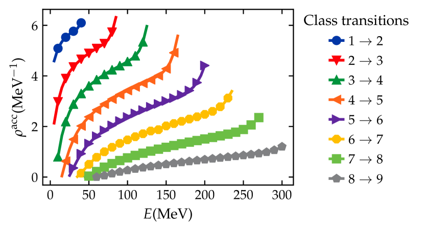
Figure 4: Density of accessible states $\rho^{\text{acc}}_{mm+1}(E)$ for case (i) (see text) in the constant-spacing model as a function of excitation energy $E$ for $A=42$ particles, $51$ single-particle states, $V=45$ MeV, $F=37$ MeV, and $\hbar\omega_{0}=5$ MeV. Colors and symbols correspond to different transitions between particle-hole classes $m\rightarrow m+1$.

The absorption of a photon of energy $\hbar\omega_{0}$ involves either one of two processes: (i) A nucleon absorbs the energy $\hbar\omega_{0}$ and is thereby promoted from a single-particle state below $F$ to a single-particle state above $F$ (without being promoted to the continuum). That causes a transition from class $(i,k,m)$ to class $(i,k+1,m+1)$. (ii) A particle absorbs the energy $\hbar\omega_{0}$ (without being promoted to the continuum), or a hole absorbs $\hbar\omega_{0}$ without exceeding the Fermi energy. That causes a transition from class $(i,k,m)$ to class $(i,k+1,m)$.

For case (i), the energy $\varepsilon$ of the nucleon prior to photon absorption must obey $F-\hbar\omega_{0}<\varepsilon<F$. The probability of finding an occupied single-particle state at energy $\varepsilon$ below $F$ is $n_{A-m,E}(\varepsilon)$, and the probability of finding an empty single-particle state with energy $\varepsilon+\hbar\omega_{0}>F$ is $(1-n_{m,E}(\varepsilon+\hbar\omega_{0}))$. The density of accessible states is, thus, given by

$$\rho^{\text{acc}}_{mm+1}(E) = \int\limits^{F}_{F-\hbar\omega_{0}}d{\varepsilon}\,n_{A-m,E}(\varepsilon)[1-n_{m,E}(\varepsilon+\hbar\omega_{0})]$$ (13)

$$\times \rho_{1}(\varepsilon)\rho_{1}(\varepsilon+\hbar\omega_{0})\ .$$

Figure 4 shows $\rho^{\text{acc}}_{mm+1}(E)$ versus energy $E$ for several values of $m$ and for parameters given in the figure caption. The density of accessible states is a monotonically increasing function of energy for all particle-hole classes. It decreases with increasing $m$ of the particle-hole class.

For case (ii) we obtain analogously

$$\rho^{\text{acc}}_{mm}(E) = \int\limits_{0}^{F-\hbar\omega_{0}}d{\varepsilon}\,n_{A-m,E}(\varepsilon)[1-n_{A-m,E}(\varepsilon+\hbar\omega_{0})]$$ (14)

$$\times \rho_{1}(\varepsilon)\rho_{1}(\varepsilon+\hbar\omega_{0})$$

$$+ \int\limits_{F}^{V-\hbar\omega_{0}}d{\varepsilon}\,n_{m,E}(\varepsilon)[1-n_{m,E}(\varepsilon+\hbar\omega_{0})]$$

$$\times \rho_{1}(\varepsilon)\rho_{1}(\varepsilon+\hbar\omega_{0})\ .$$

For the same set of parameters as used in Fig. 4, Fig. 5 shows results for $\rho^{\text{acc}}_{mm}(E)$ versus $E$ for several values of $m$. For large $E$ that function decreases with increasing $E$. For such energies, the sparseness of empty levels makes it increasingly difficult to add the energy $\hbar\omega_{0}$ to a particle or a hole. That effect is absent in $\rho^{\text{acc}}_{mm+1}(E)$.

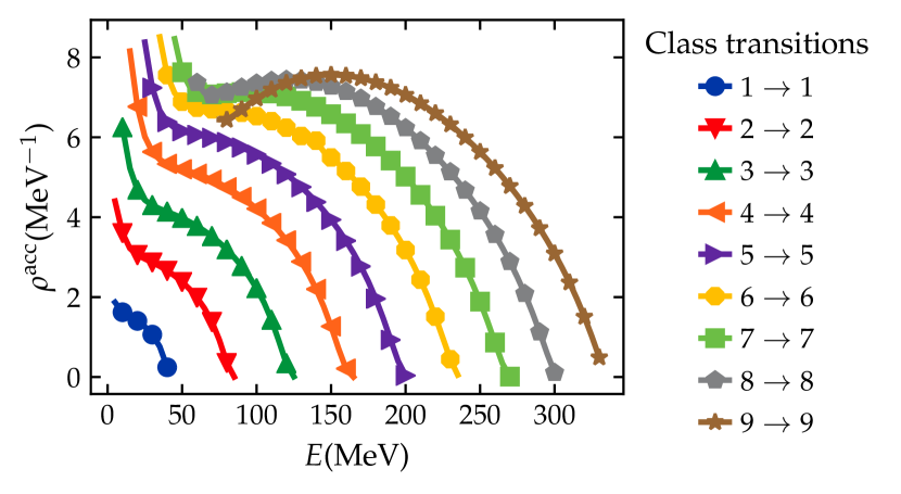
Figure 5: Density of accessible states $\rho^{\text{acc}}_{mm}(E)$ for case (ii) (see text) in the constant spacing model as a function of excitation energy $E$. We use the same parameters as for Fig. 4. Colors and symbols correspond to transitions within different particle-hole classes $m$.

III Numerical Results

We calculate the time-dependent occupation probabilities $P_{m}(i,k,t)$ for two medium-weight target nuclei, $A=42$ and $A=100$, that interact with a short pulse of MeV photons. These nuclei are taken to be generic for their range of mass values. We solve Eq. (1) numerically for several choices of the effective dipole width $\widetilde{\Gamma}_{\rm dip}$ and of the length $(n+1)$ of the decay chain. Equation (1) is written in matrix form as $\dot{P}=\mathcal{M}P$. The elements of the column vector $P$ are the occupation probabilities $P_{m}(i,k,t)$ labeled by an overall index $j$ covering the set $(i,k,m)$. The initial condition $P_{m}(i,k,0)=\delta_{i,0}\delta_{k,0}\delta_{m,0}$ mimics the ground state of the target nucleus. The matrix $\mathcal{M}$ is independent of time. The number of elements in $\mathcal{M}$ ranges from $670$ for $A=42$ to $\sim 10000$ for $A=100$ per neutron decay generation. These elements vary over 8 orders of magnitude for nuclei with mass number $A=42$, and over 70 orders of magnitude for nuclei with mass number $A=100$. Diagonalization of this matrix, therefore, poses a stiff problem. As in Ref. Pálffy et al. (2015) we treat the extremely stiff differential equations (1) via a matrix exponential method. We use the Chebyshev rational approximation method (CRAM) which is known for its success in solving burnup equations Pusa (2011, 2016). For all the calculations we use CRAM with partial fraction decomposition and an approximation of order 20 Pusa (2011). Despite the efficiency of CRAM, the size and stiffness of the matrix $\mathcal{M}$ restricts our present calculations to nuclear mass numbers $A\leq 100$.

Our numerical calculations yield values for the occupation probability $P_{m}(i,k,m)$. In the contour plots for $P_{m}(i,k,m)$ we convert $k$ to energy $E$ via $E=k\hbar\omega_{0}$. We use $\hbar\omega_{0}=5$ MeV throughout. This value lies well within the planned range of the Extreme Light Infrastructure Extreme Light Infrastructure Nuclear Physics (2019) (ELI-NP) and the Gamma Factory Płaczek et al. (2019) facilities mentioned in the Introduction.

III.1 Light medium-weight nuclei ($A=42$)

We first consider the comparatively simple case of small nucleon number $A=42$ and constant level density $\rho_{1}(\varepsilon)\equiv\mathrm{const}=A/F$ with $51$ single-particle states. Figure 6 shows the occupation probabilities versus time and excitation energy for the target nucleus in the absence of neutron decay ($\Gamma_{N}=0$) for $\widetilde{\Gamma}_{\mathrm{dip}}=5$ MeV and a duration time of the laser pulse $1/\sigma=20$ zs. During the process, particle-hole classes up to $m=9$ are populated, with the higher $m$-values requiring larger excitation energy.

A cut in the contour spectra of Fig. 6 at $t=20$ zs (i.e., at the end of the laser-nucleus interaction) is shown in Fig. 7. For each class $m$ of particle-hole numbers, the occupation probabilities display a maximum. It occurs at the energy for which the rates of dipole absorption and stimulated dipole emission are equal. There the particle-hole level density $\rho_{m}(0,k)$ has its maximum. Beyond that peak, stimulated dipole emission outweighs dipole absorption, the excitation process saturates, and further excitation becomes increasingly unlikely. Inspection of Fig. 6 shows that prior to termination of the pulse at $t=20$ zs, classes $m=5$ and $m=6$ are closer to saturation (the occupation probabilities run parallel to the abscissa) than classes with higher values of $m$. We conclude that for different classes saturation is achieved at different times, and the system as a whole is saturated when the “slowest” class is saturated.

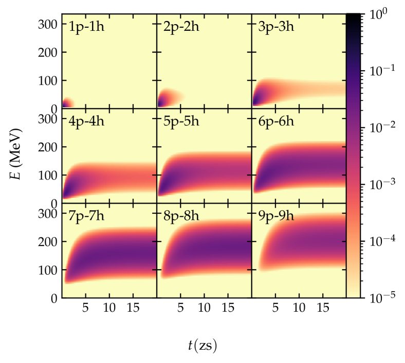
Figure 6: Contour plots of the time-dependent occupation probabilities $P_{m}(0,k,t)$ of a light medium-weight nucleus with $A=42$ as a function of excitation energy $E$ for the accessible particle-hole classes. Neutron evaporation is not included. The parameters used are given in the text.

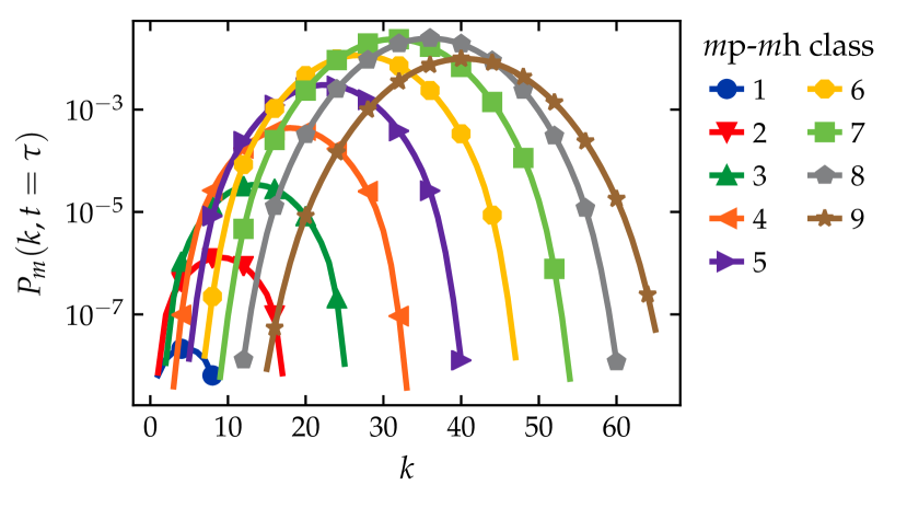
Figure 7: A cut through the contour plots in Fig. 6 at the termination $t=20$ zs of the laser pulse. The occupation probabilities are shown as functions of the number of absorbed photons $k$ for different particle-hole classes.

Figure 8 shows the total occupation probability $P(0,k,t)=\sum_{m}P_{m}(0,k,t)$ of the target nucleus. Qualitatively, that plot is similar to the quasiadiabatic results in Ref. Pálffy et al. (2015).

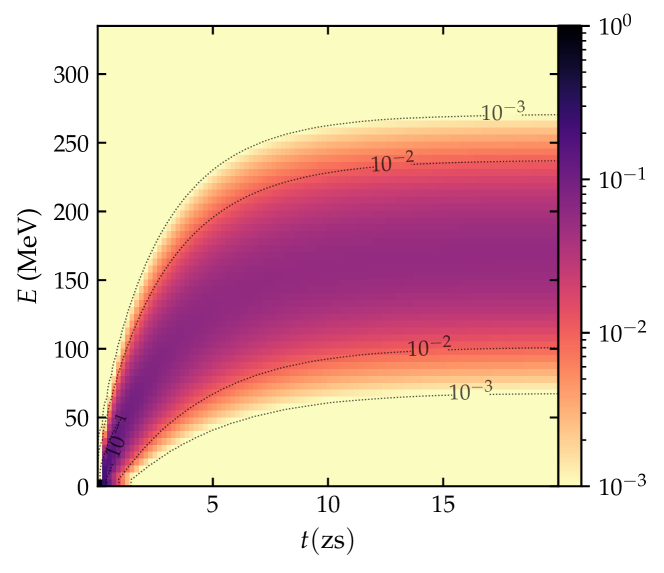
Figure 8: Contour plot of the time-dependent total occupation probability as a function of excitation energy $E$ and time $t$ for dipole absorption and stimulated emission only (no neutron decay). We use the same parameters as in Fig. 6 (see text).

III.2 Medium-weight nuclei $(A=100$)

For mass number $A=100$ we use the single-particle level density in Eq. (10). With a depth $V=45$ MeV of the single-particle potential, that gives a total of $148$ single-particle states. The increase in both particle number and number of states causes a significant increase in the dimension of the matrix ${\cal M}$. Fortunately, many matrix elements are zero and one can exploit that sparseness to reduce the matrix dimension. The resulting matrix for the target nucleus has dimension 5328. The resulting matrix for $n=4$ generations of nuclei has dimension 21088.

Our calculations were performed for pulse durations of 40 zs and for four choices of the effective dipole width, $\widetilde{\Gamma}_{\rm dip}=$1, 5, 10, and 20 MeV. We focus attention on $\widetilde{\Gamma}_{\rm dip}=20$ MeV (typical for the sudden regime) and on $\widetilde{\Gamma}_{\rm dip}=5$ MeV (relevant for a comparison with results for the quasiadiabatic regime in Ref. Pálffy et al. (2015)).

For $A=100$, particle-hole classes up to $m=48$ can be reached. For a better understanding of our results we first show in Fig. 9 the density of states versus $k$ for every fourth particle-hole class. The excitation energy is given by the number $k$ of absorbed photons, each with energy $\hbar\omega_{0}=5$ MeV. Particle-hole classes with small (large) $m$ dominate at small (large) energies, respectively. Densities with $m\approx 30$ have the largest values. The total density (summed over all particle-hole classes) is the envelope to these curves, with a maximum at $\approx 575$ MeV.

III.2.1 No Neutron Evaporation

We first focus attention on the time evolution of the target nucleus, disregarding neutron evaporation. Fig. 10 presents the occupation probabilities as functions of time and excitation energy for $\widetilde{\Gamma}_{\rm dip}=20$ MeV. To be able to display the populations of low $m$ and high $m$ particle-hole classes in the same plot, the scale ranges from $10^{-7}$ to unity and comprises two orders of magnitude more than the plot of Fig. 6. Classes with small numbers of particle-hole pairs are populated in the first stages of photoexcitation. Classes with $m$ between $23$ and $37$ are then occupied rapidly and stay populated until the end of the laser pulse. The classes with the highest particle-hole numbers are populated poorly and only late when sufficient energy was transferred to reach the domain of excitation energy where their densities are large. Figure 9 shows that these densities reach their maxima at an energy higher than the saturation energy, that these maxima are lower than those of the middle classes, and that these maxima strongly decrease with increasing $m$ beyond the 36p-36h class. That is in contrast to the case of constant spacing; cf. Fig. 6 where the maximum of the level density for the highest 9p-9h class is not significantly smaller than that of the neighboring 8p-8h class which dominates all the other classes.

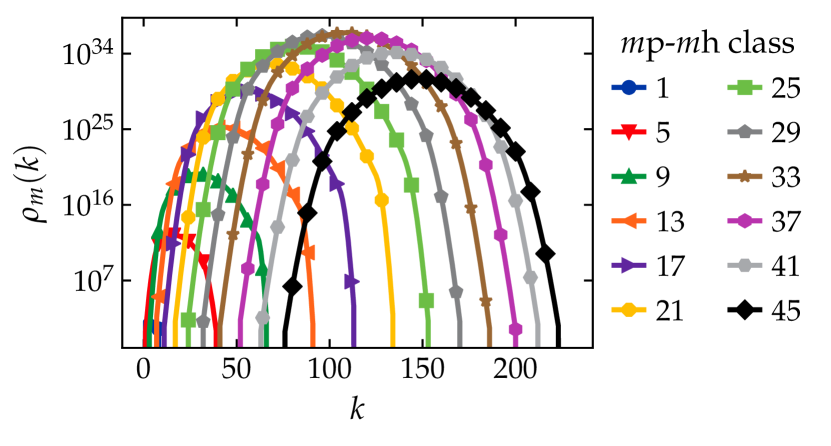
Figure 9: Level densities $\rho_{m}(0,k)$ for a medium-weight nucleus $A=100$ as functions of excitation energy (measured in units of the number $k$ of absorbed photons). For clarity of illustration we present the densities only for every fourth particle-hole class.

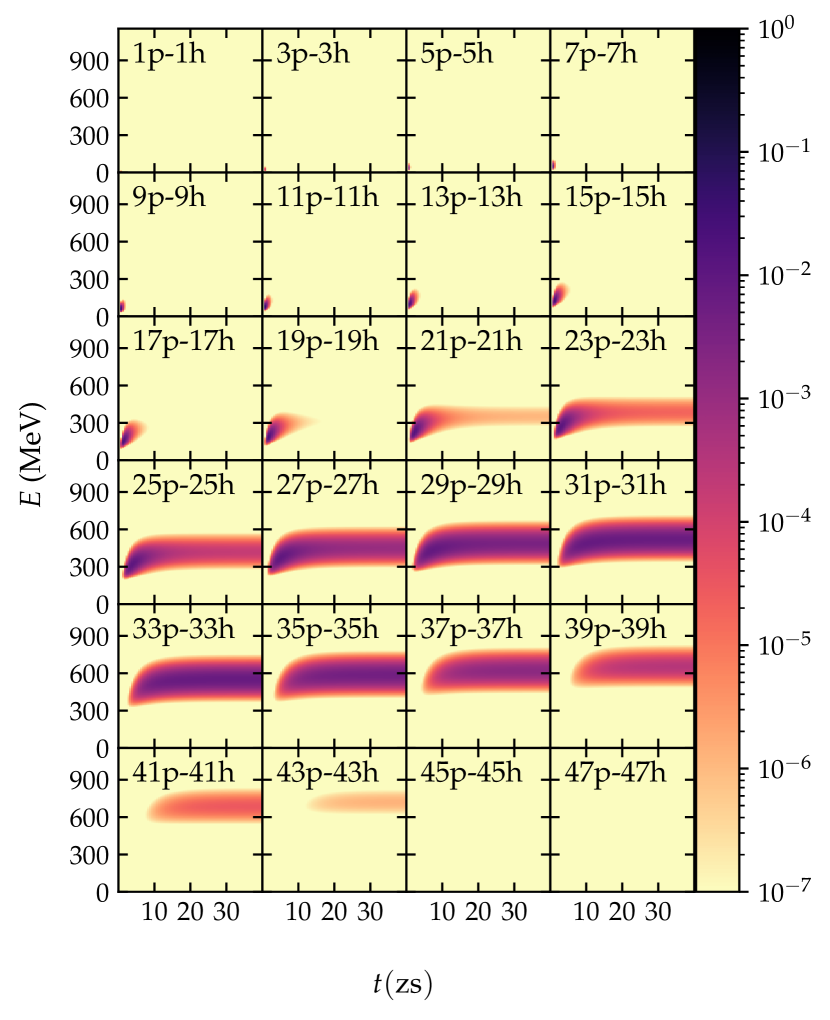
Figure 10: Contour plots of the time-dependent occupation probabilities $P_{m}(0,k,t)$ for every second accessible particle-hole class from $1$p-$1$h to $47$p-$47$h as functions of excitation energy $E$ for dipole absorption and stimulated emission only (no neutron emission). The parameters are mass number $A=100$, the single-particle level density as given in Eq. (10), $\widetilde{\Gamma}_{\mathrm{dip}}=20$ MeV, and $\tau=40$ zs.

Figure 10 shows that all classes reach saturation. The same is true for the total occupation probability $P(0,k,t)=\sum_{m}P_{m}(0,k,t)$ shown in Fig. 11(a). Saturation is reached at $t\approx 20$ zs, and $P(0,k,t)$ remains constant thereafter. We note the qualitative similarity with results obtained in Ref. Pálffy et al. (2015) for the quasiadiabatic regime. It is interesting to note that the total occupation probability is sensitive to the mechanism of photoabsorption. Indeed, allowing only for the processes described in Fig. 2 (change of particle-hole class for each photon absorption or emission process), the time scale for excitation increases dramatically. Figure 11(b) shows the total occupation probability calculated using $m^{\prime}=m\pm 1$ only in the dipole excitation and emission part of Eq. (1) for $\widetilde{\Gamma}_{\mathrm{dip}}=20$ MeV. Comparison with Fig. 11(a) shows the increase of the time scale for photoexcitation. Saturation is not yet reached even at $t=40$ zs.

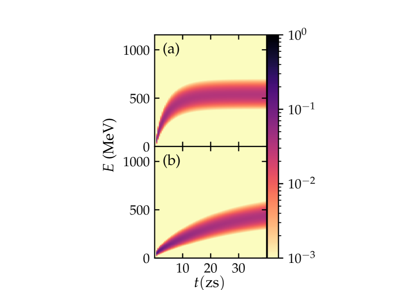
Figure 11: Contour plots of the time-dependent total occupation probabilities $P(0,k,t)$. (a) Photon absorption or emission allows for the two possible processes presented in Figs. 2 and 3. (b) Photon absorption or emission allows only for the process in Fig. 2. The parameters are the same as in Fig. 10.

Figure 12 presents contour plots of the total occupation probabilities for four choices of the effective dipole width, $\widetilde{\Gamma}_{\mathrm{dip}}=$ 1, 5, 10, and 20 MeV. The comparison shows whether and how quickly saturation is reached. For $\widetilde{\Gamma}_{\mathrm{dip}}=1$ MeV and $\widetilde{\Gamma}_{\mathrm{dip}}=5$ MeV saturation requires duration times longer than the pulse duration 40 zs used. For $\widetilde{\Gamma}_{\mathrm{dip}}=10$ MeV saturation is reached at 40 zs, and for $\widetilde{\Gamma}_{\mathrm{dip}}=20$ MeV, it is not possible to further transfer energy into the nucleus for times $t\geq 20$ zs. Comparing with the case of $A=42$, $\widetilde{\Gamma}_{\mathrm{dip}}=5$ MeV, and constant single-particle level spacing shown in Fig. 8, we notice that for $A=100$ the same effective dipole rate $\widetilde{\Gamma}_{\mathrm{dip}}=5$ MeV does not bring the nucleus to the same degree of saturation at $t=20$ zs. Saturation requires either a longer duration time of the laser pulse or a greater effective dipole rate. That is because saturation in the nucleus $A=100$ occurs at a substantially higher energy. For $A=42$ (for $A=100$), the maximum of the total level density is at $165$ MeV (at $533$ MeV, respectively). [For $A=100$ and for the single-particle level density as given in Eq. (10), the total level density is a slightly asymmetric function of energy].

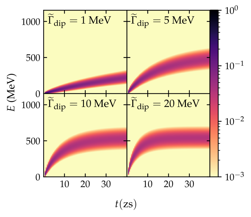
Figure 12: Contour plots of the total time-dependent occupation probabilities $P(0,k,t)$ versus time $t$ and excitation energy $E$ for four values of $\widetilde{\Gamma}_{\mathrm{dip}}$ as indicated. The other parameters are the same as in Fig. 10.

To compare results for different effective dipole widths we use the total excitation energy $E_{\rm tot}(t)=\hbar\omega_{0}\sum_{k,m}kP_{m}(0,k,t)$ of the nucleus at time $t$, and the time interval $\Delta_{1}t(E)=t(E+\hbar\omega_{0})-t(E)$, where $t(E)$ is the earliest time at which the total energy $E$ is reached. At very short times, $E_{\rm tot}(t)$ grows linearly with time $t$, and $\Delta_{1}t$ is a measure of the time interval between the successive absorption of two photons. With increasing excitation energy stimulated emission becomes important, $E_{\rm tot}(t)$ grows less strongly than linearly, and $\Delta_{1}t$ increases correspondingly. Figure 13 shows $E_{\rm tot}$ and $\Delta_{1}t$ as functions of time for $\widetilde{\Gamma}_{\mathrm{dip}}=5$ MeV and $\widetilde{\Gamma}_{\mathrm{dip}}=20$ MeV. As expected, at short times $E_{\rm tot}(t)$ increases significantly faster for the bigger of the two effective dipole rates. The time between two successive photon absorption processes is correspondingly shorter and, thus, more competitive with the nuclear relaxation time. We have to keep in mind, however, that the relaxation time itself becomes shorter, too, with increasing excitation energy. Moreover, Fig. 13 shows that induced photon emission and, eventually, saturation become important very early for $\widetilde{\Gamma}_{\mathrm{dip}}=20$ MeV, so that $\Delta_{1}t$ ceases to be a measure of the time interval between successive photon absorption processes.

III.2.2 Comparison with the quasiadiabatic case

In the quasiadiabatic regime, equilibration is instantaneous. Only total level densities and total occupation probabilities enter the calculation. If in the sudden regime the dipole width $\widetilde{\Gamma}_{\mathrm{dip}}$ is so small that equilibration happens between each pair of subsequent photon processes, our values for the total occupation probabilities must agree with the ones calculated for the quasiadiabatic regime. In Fig. 14 we compare our total occupation probabilities for $\widetilde{\Gamma}_{\mathrm{dip}}=5$ MeV and 100-zs pulse duration with results from Ref. Pálffy et al. (2015). The parameters are the same as in our case with one exception. The dipole matrix element used in the quasiadiabatic calculation differs from that of the present calculation by a factor 2.3 because its definition involves a different 1p-1h density $\rho_{1}(0,1)$; see Ref. Obložinský (1986). In Fig. 14 we have accounted for that difference. The figure shows snapshots of the occupation probability at four time instants, $t=2,\,10,\,40$, and $100$ zs. The results display good agreement. Slight differences in the wings can be attributed to the different strategies to calculate the tails of the level densities used here and in Ref. Pálffy et al. (2015). The two calculations agree only if in our calculation photon absorption and emission both without and with change of particle-hole class as shown in Figs. 2 and 3 are included.

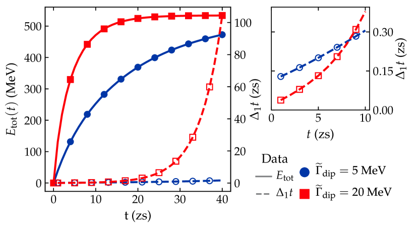
Figure 13: Total excitation energy $E_{\rm tot}$ (solid lines, left vertical axis) and approximate time interval between two photon absorptions $\Delta_{1}t$ (dashed lines, right vertical axis) as a function of time for $\widetilde{\Gamma}_{\mathrm{dip}}=5$ MeV (blue circles) and $\widetilde{\Gamma}_{\mathrm{dip}}=20$ MeV (red squares). The inset zooms in the interval of the first 10 zs for $\Delta_{1}t$.

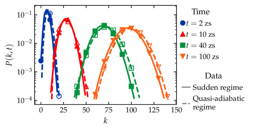
Figure 14: Total occupation probabilities (solid lines) compared with results from Ref. Pálffy et al. (2015) for the quasiadiabatic regime (dashed lines) as a function of the number $k$ of absorbed photons at times $t=$ 2, 10, 40, and 100 zs and for $\widetilde{\Gamma}_{\mathrm{dip}}=5$ MeV.

For the generic value $\Gamma^{\downarrow}=5$ MeV of the spreading width for medium-weight nuclei, the nuclear relaxation time would be $1/\Gamma^{\downarrow}\simeq 0.13$ zs. However, our calculations using the rates of Sec. II.2.1 show that the relaxation time actually depends on energy and particle-hole configuration and ranges from less than 1 zs to a few zs. That indicates that for short times (i.e., at the beginning of the laser pulse), photon absorption is faster than equilibration. As a test, we compare in Fig. 15 the occupation probabilities $P_{m}(0,k,t)$ obtained in our calculation with equilibrium values $P^{\rm eq}_{m}(0,k,t)=\rho_{m}(0,k)P(0,k,t)/\rho(0,k)$. Here $\rho(0,k)$ is the total level density and $P(0,k,t)$ is the total occupation probability at energy $k$. We do so for $\widetilde{\Gamma}_{\mathrm{dip}}=5$ and $20$ MeV, for three instants of time ($t=2,\,5$, and $10$ zs), and for a range of $k$ values (or excitation energies) and $m$ values. We display the relative difference $R_{m}(k)=2[P^{\rm eq}_{m}(0,k,t)-P_{m}(0,k,t)]/[P^{\rm eq}_{m}(0,k,t)+P_{m}(0,k,t)]$ in a contour plot. With increasing excitation energy $E$ (or increasing $k$), the total number of classes $(0,k,m)$ increases strongly whereas each absorbed photon creates at most one additional particle-hole pair. Therefore we expect that for fixed $k$ and prior to equilibrium, classes with small $m$ (large $m$) are overpopulated (underpopulated), corresponding to $R_{m}(k)<0$ ($R_{m}(k)>0$, respectively). That expectation is actually met for $\widetilde{\Gamma}_{\mathrm{dip}}=5$ MeV, small time $t=2$ zs (upper left panel of Fig. 15) and for excitation energies up to $\approx 100$ MeV. The dashed line corresponds to a process where each photon of energy $\hbar\omega_{0}=5$ MeV generates an additional particle-hole pair. A similar pattern can be observed also for $t\simeq 0.5$ zs for $\widetilde{\Gamma}_{\mathrm{dip}}=20$ MeV, though not displayed in Fig. 15.

At first surprisingly, for all other data shown in the figure our expectation fails, and the pattern is actually reversed. The occupation probabilities at fixed excitation energy are largest for classes with large particle-hole numbers. The behavior of the density of accessible states $\rho^{\text{acc}}_{mm}(E)$ in Fig. 5 explains why this happens. The densities of accessible states $\rho^{\text{acc}}_{mm}(E)$, and the associated dipole rates, are largest for classes with large particle-hole numbers. Once equilibration provides a sufficient minimum value for the occupation probabilities of large-$m$ classes, these classes are responsible for the bulk of dipole absorption. It appears that at that time the excitation processes within the same class described by $\rho^{\text{acc}}_{mm}(E)$ prevails over the excitation generating additional particle-hole pairs. This situation is reached at about $100$-MeV excitation energy in the upper left-hand panel of Fig. 15. The overall tendency of dominant excitation of the large-$m$ classes would be amplified with every dipole absorption process. However, each absorbed photon promotes the nucleus to higher energy where the level densities $\rho_{m}(i,k)$ and, thus, also the rates for equilibration become larger. For that same reason, equilibration is faster for $\widetilde{\Gamma}_{\mathrm{dip}}=20$ MeV. Here the difference between the underpopulation of small $m$ values and the overpopulation of large $m$-values is less pronounced at $t=5$ zs and has almost disappeared at $t=10$ zs. The center region of equilibrated occupation probabilities where $R_{m}(k)\approx 0$ has the shape of a stripe which runs almost parallel to but below the line $k(m)$ (not illustrated) defined by the $k$ value where the density $\rho_{m}(0,k)$ versus $m$ has its maximum. As time increases, that central equilibrated stripe becomes wider, and it becomes more steep than the line $k(m)$.

Generally speaking, the occupation probabilities $P_{m}(0,k,t)$ deviate most strongly from equilibrium at short times ($t\leq 2$ zs) and, with increasing time, tend towards equilibrium. That is expected and is true for both values of the effective dipole width. Equilibration becomes faster as energy increases while saturation slows photon absorption. The difference between the quasiadiabatic and the sudden regime is, therefore, manifest mainly at short times and at comparatively low excitation energies and fades away as the nucleus approaches saturation. We conclude that as long as neutron emission is not taken into account, the sudden regime is quite similar to the quasiadiabatic regime, except for the initial phase of the process.

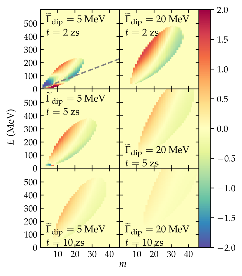
Figure 15: Relative difference $R_{m}(k)=2[P^{\rm eq}_{m}(0,k,t)-P_{m}(0,k,t)]/[P^{\rm eq}_{m}(0,k,t)+P_{m}(0,k,t)]$ as a function of excitation energy $E$ and particle-hole class $m$. We consider snapshots at $t=5,\,10$ and $20$ zs for effective dipole absorption rates $\widetilde{\Gamma}_{\mathrm{dip}}=5$ MeV and $20$ MeV. The dashed line shows the function $E(m)=m\hbar\omega_{0}$ with $\hbar\omega_{0}=5$ MeV. See text for further explanations.

III.2.3 Neutron evaporation

To include neutron evaporation we consider the target nucleus ($A=100$, $i=0$) plus three daughter nuclei with mass numbers $A=99$, $A=98$, and $A=97$ ($i=1,2$, and $3$, respectively). We disregard neutron emission of the last nucleus with mass number $A=97$ which, thus, serves as a dump for the overall probability flow. Our numerical results show that the contributions owing to $m^{\prime}=m$ and to $m^{\prime}=m-1$ in Eq. (8) are almost equal. This is illustrated in Fig. 16 presenting the respective total occupation probabilities as a function of the number of absorbed photons $k$ for $i=0$ and $\widetilde{\Gamma}_{\mathrm{dip}}=5$ MeV. That comparison looks similar for $i=1,2,3$.

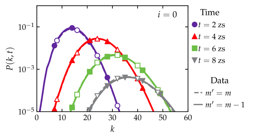
Figure 16: Comparison of total occupation probabilities for target nucleus ($i=0$) summed over all particle-hole classes as a function of the number $k$ of absorbed photons at times $t=$ 2, 4, 6, and 8 zs. We calculate the neutron decay rates considering only $m^{\prime}=m$ (dashed lines) or only $m^{\prime}=m-1$ (solid lines). We use $\widetilde{\Gamma}_{\mathrm{dip}}=5$ MeV.

In the following we therefore simplify the calculation by considering the term $m^{\prime}=m$ only. The results for $\widetilde{\Gamma}_{\mathrm{dip}}=5$ MeV and $\widetilde{\Gamma}_{\mathrm{dip}}=20$ MeV are presented in Figs. 17 and 18, respectively. Because the relevant neutron evaporation decays take place within the first few zs, we consider here a pulse duration time of $20$ zs. Both figures are qualitatively similar to the quasiadiabatic case. Neutron evaporation sets in at energies much lower than saturation, interrupting the sequence of photoabsorption processes. In Fig. 17, the occupation probability of the target nucleus is lost by neutron decay already at $t=7$ zs, and the occupation probabilities of nuclei with $i=1$ and $i=2$ become significant. In comparison, for $\widetilde{\Gamma}_{\mathrm{dip}}=20$ MeV (Fig. 18) the occupation probability of the target nucleus reaches higher energies more quickly and is completely depleted at $\approx$ 3.5 zs, which is about a factor 2 sooner than for $\widetilde{\Gamma}_{\mathrm{dip}}=5$ MeV. That trend is also seen for the nuclei with $i=1$ and $i=2$. By construction, in the present calculation neutron decay does not change particle-hole class. The equilibration in the daughter nucleus is therefore similar to the one in the parent, modified only by the change of excitation energy from the loss of one neutron.

We expect qualitatively similar results for a longer chain of neutron evaporation processes. Neutron decay prevents the nuclei in the chain from reaching saturation. The length of the actual chain depends on the duration of the laser pulse. In any case we expect that laser irradiation leads to proton-rich medium-weight nuclei at high excitation energy. The probability distribution of the nuclei in the chain depends upon the parameters of the laser pulse. Once experimental data become available, such details can be explored further by calculations as performed in the present paper.

We compare our results for the chain of four nuclei with $i=0,1,2,3$ with corresponding results for the quasiadiabatic regime in Ref. Pálffy et al. (2015). These were done for $\widetilde{\Gamma}_{\mathrm{dip}}=5$ MeV but with a different 1p-1h density $\rho_{1}(0,1)$ that was taken from Ref. Obložinský (1986). We adjust our calculations correspondingly. For the target nucleus, the occupation probabilities are very similar in the sudden and in the quasiadiabatic calculation (without considering neutron evaporation). Neutron evaporation occurs slightly faster in the quasiadiabatic regime. Inspection of the quantities $\sum_{m}\Gamma_{N}(i,k,m)\rho_{m}(i,k)/\rho(i,k)$ and $\Gamma_{N}(i,k)$, where $\rho(i,k)$ and $\Gamma_{N}(i,k)$ are the level density and total neutron evaporation rate in Ref. Pálffy et al. (2015), respectively, shows that indeed between $k=10$ and $k=30$, neutron evaporation is stronger in the quasiadiabatic regime. The difference is largest at $\approx$ $E=68$ MeV. In Ref. Pálffy et al. (2015), tails of the level density up to an excitation energy of 68 MeV were calculated using the Bethe formula Bethe (1936) while the central part was calculated using the approach of Ref. Pálffy and Weidenmüller (2013b) also employed here. Because of that procedure the level density $\rho(i,k)$ of the quasiadiabatic approach has a kink at $E=68$ MeV. Such a kink does not appear in the present work where we extrapolate the level density in the tails. We conclude that the observed difference in the neutron evaporation rate is related to the different method used in calculating the level densities at small energies. With this proviso we conclude that for $\widetilde{\Gamma}_{\mathrm{dip}}=5$ MeV, the present calculation confirms the previous results in Ref. Pálffy et al. (2015) for the quasiadiabatic regime. It is clear, nevertheless, that the occupation probabilities in the decay chain are sensitive to details of the calculation such as the precise form of the level densities and the manner in which photon absorption and stimulated photon emission changes the occupation of the particle-hole classes. Future experiments are yet to confirm the correct assumptions required for more quantitative estimates.

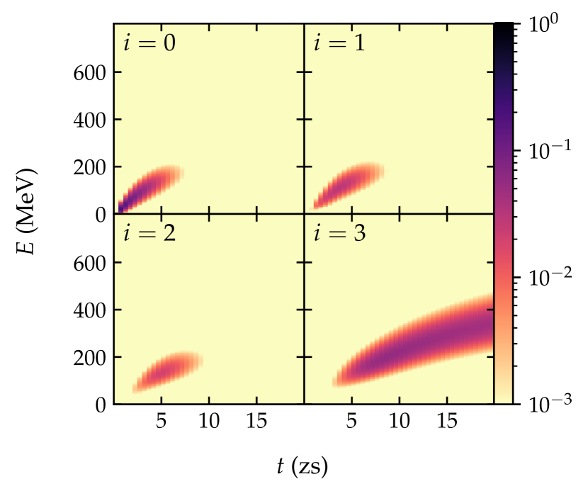
Figure 17: Contour plots of the time-dependent occupation probabilities summed over all particle-hole classes as a function of excitation energy $E$ for target nucleus ($i=0$) and three generations of daughter nuclei ($i=1,2,3$). The parameters are the mass number $A=100$, Eq. (10) for the single-particle level density, $\widetilde{\Gamma}_{\mathrm{dip}}=5$ MeV, $\tau=20$ zs and $\hbar\omega_{0}=5$ MeV.

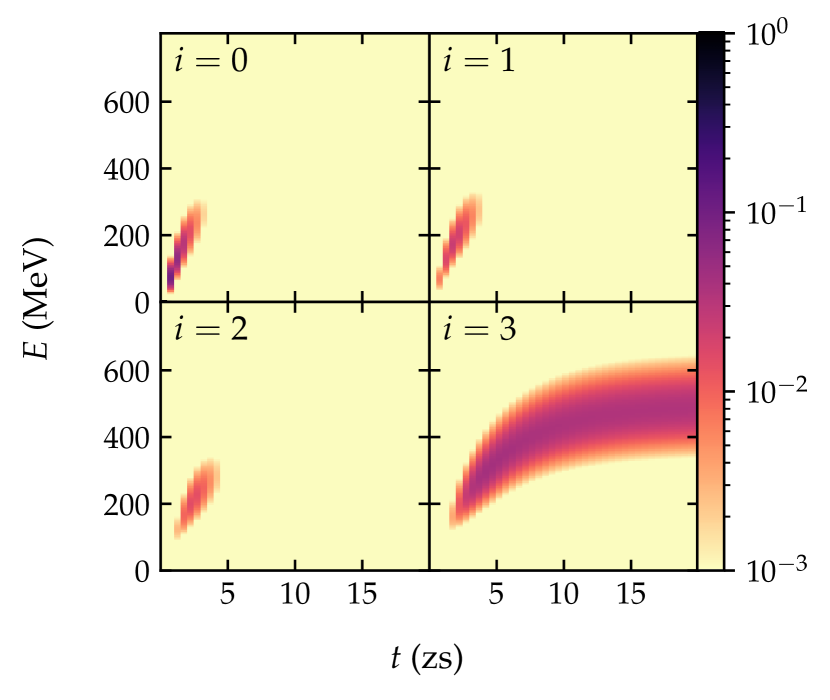
Figure 18: The same as in Fig. 17 for $\widetilde{\Gamma}_{\mathrm{dip}}=20$ MeV.

IV Summary and Discussion

Previous work on the laser-nucleus interaction Pálffy and Weidenmüller (2014); Pálffy et al. (2015) was focused on the quasiadiabatic regime where the compound nucleus equilibrates after each photoabsorption process. For the theoretical modeling, it suffices to use the total level density at fixed excitation energy. In the present paper we have investigated the sudden regime where equilibration is incomplete. That regime requires a more detailed modeling. We use classes of particle-hole states and assume that within each class, equilibration is instantaneous. That assumption is required to justify a statistical modeling and the use of rate equations. The interaction between classes at the same excitation energy leads to equilibration. Equilibration competes with multiple photon absorption and induced photon emission. We also allow for neutron evaporation feeding a chain of proton-rich nuclei.

In the absence of neutron evaporation and for a comparatively small value $\widetilde{\Gamma}_{\mathrm{dip}}=5$ MeV of the effective dipole width, equilibration competes successfully with dipole absorption, and our results are in good agreement with those for the quasiadiabatic regime of Ref. Pálffy et al. (2015). For $\widetilde{\Gamma}_{\mathrm{dip}}=20$ MeV, on the other hand, the occupation probabilities of the particle-hole classes deviate markedly from their equilibrium values in the beginning stages of the multi-photon absorption process. In later stages, they approach the equilibrium values, and the resulting excitation pattern becomes qualitatively similar to that of the quasiadiabatic regime. That happens before saturation (caused by the equality of the rates for dipole absorption and induced dipole emission) limits the further increase of excitation energy. Neutron evaporation actually sets in long before saturation, depletes the target nucleus, and feeds a chain of proton-rich nuclei. Repeated neutron evaporation somewhat decreases the excitation energy and slows down the path to saturation for each nucleus in the decay chain.

Throughout the paper we have neglected both fission and direct emission of nucleons by photoabsorption into the continuum. As shown in Ref. Pálffy and Weidenmüller (2014), these processes play only a minor role for nuclei around $A=100$, but may be competitive with neutron decay for heavier nuclei. The effects of fission for $A=200$ were investigated in more detail in Ref. Pálffy et al. (2015) for the quasiadiabatic regime. The effective charges of neutrons and protons being nearly equal in magnitude, direct photoabsorption might still be of interest also for medium-weigth nuclei, especially for $\widetilde{\Gamma}_{\mathrm{dip}}=20$ MeV. That process would populate highly excited states not only in the chain of proton-rich nuclei reached by neutron emission, but also in all nuclei that lie between the valley of stability and nuclei in the chain.

All our calculations were done for photons with energy $\hbar\omega_{0}=5$ MeV. Doubling that energy would lift it above the nucleon binding energy. That would substantially increase direct photoabsorption processes and might lead to a significant loss of mass.

The sudden regime is bounded by a regime where dipole excitation is so strong that equilibration is altogether excluded. Then our assumption that within every class of particle-hole states equilibration is instantaneous fails. Multiple dipole excitation generates pairs of more or less independent particle-hole states. It would be of substantial interest to investigate the transition of the compound nucleus from a strongly interacting system (realized in the adiabatic regime) to a system of nearly independent particles (realized in the extreme sudden regime of the laser-nucleus interaction).