SimpleMKKM: Simple Multiple Kernel K-means

Abstract

We propose a simple yet effective multiple kernel clustering algorithm, termed simple multiple kernel $k$-means (SimpleMKKM). It extends the widely used supervised kernel alignment criterion to multi-kernel clustering. Our criterion is given by an intractable minimization-maximization problem in the kernel coefficient and clustering partition matrix. To optimize it, we re-formulate the problem as a smooth minimization one, which can be solved efficiently using a reduced gradient descent algorithm. We theoretically analyze the performance of SimpleMKKM in terms of its clustering generalization error. Comprehensive experiments on 11 benchmark datasets demonstrate that SimpleMKKM outperforms state of the art multi-kernel clustering alternatives.

1 Introduction

In multiple kernel clustering (MKC) (Zhao et al., 2009), we aim to combine a set of pre-specified kernel matrices to improve clustering performance. These kernel matrices could encode heterogeneous sources or views of the data (Yu et al., 2012). One popular method, multiple kernel $k$-means(MKKM) (Huang et al., 2012), has been studied intensively and used in various applications (Yu et al., 2012; Gönen & Margolin, 2014; Liu et al., 2019; Peng et al., 2019; Kumar & Daumé, 2011; Kumar et al., 2011). The approach is attractive also from a theoretical perspective, as it unifies the search of the optimal base kernel coefficient and the clustering partition matrix into a single objective function, which is usually solved by using two-step alternating optimization on the coefficients and clustering partition matrix.

Several variants of MKKM have been developed to further improve the clustering performance (Yu et al., 2012; Gönen & Margolin, 2014; Li et al., 2016; Liu et al., 2016b, 2017a, 2019). Notably, Gönen & Margolin (2014) substantially increase the expressiveness of MKKM by allowing for a locally adaptive kernel mixtures, which can better capture sample-specific characteristics of the data. Li et al. (2016) propose an extension that optimizes a localized kernel alignment criterion. It aligns the local density of the samples given by the $k$-nearest neighbours with an ideal similarity matrix. This alignment helps to keep neighbouring sample pairs together, which avoids unreliable similarity evaluation. Observing that existing MKKM algorithms do not sufficiently consider the correlation among these kernels, Liu et al. (2016b) employ matrix regularization to reduce the redundancy and enhance the diversity of the selected kernels. Most of existing MKKM algorithms assume that the optimal kernel is a linear combination of a group of base kernels. This assumption is challenged in Liu et al. (2017a), who propose an optimal neighborhood kernel clustering (ONKC) algorithm to enhance the representability of the optimal kernel and strengthen the negotiation between kernel learning and clustering. More recently, MKKM algorithms have been extended to handle missing views (Liu et al., 2019). By assuming the optimal kernel is a linear combination of the base kernel matrices, Bang et al. (2018) develop a minimization-maximization framework that aims to be robust to adversarial perturbation. All these variants potentially improve standard MKKM and achieve promising clustering performance in various applications.

The objective functions of the mentioned methods differ, but they all share one commonality: they learn the kernel coefficient and the clustering partition matrix jointly. By this way, the leaned kernel coefficient can best serve the clustering, leading to superior clustering performance. However, simultaneously solving for the kernel coefficients and the clustering partition is intractable. One commonly adopted remedy is to decouple the optimization of the kernel coefficients and the clustering partition through a block coordinate descent algorithm, which optimizes the two alternately. This means, one block of variables is minimized while the other is kept fixed. However, such alternate optimization algorithms can get trapped into a local optima of the objective function. As a remedy, Liu et al. (2016b); Li et al. (2016) propose regularization strategies to avoid getting trapped into local minimum. The incorporation of these regularization terms comes at a price: the approach has additional hyper-parameters, which are difficult to select, given the unsupervised nature of clustering tasks.

In this paper, we propose Simple MKKM (SimpleMKKM)—a novel formulation for multiple kernel clustering that addresses the aforementioned shortcomings. Unlike previous approaches, SimpleMKKM optimizes the unsupervised kernel alignment criterion directly. Specifically, it minimizes kernel alignment with respect to the kernel coefficient and maximizes it with respect to the clustering matrix. This minimization-maximization optimization problem cannot readily be solved using existing alternate optimization frameworks. However, we show that this min-max problem actually leads to a more efficient and effective optimization algorithm. Specifically, we reformulate the min-max problem as a minimization problem, whose objective relies on the known optimal solution to kernel $k$-means. We then prove the differentiability of the optimal value function and calculate its reduced gradient. This leads to a solution using a reduced gradient descent algorithm, without alternating optimization. We show a generalization error bound for our approach, thus theoretically guaranteeing its clustering performance. We conduct comprehensive experiments on eleven benchmark datasets, where we compare SimpleMKKM to eight baseline methods in terms of three common evaluation criteria. We observe that SimpleMKKM consistently outperforms its competitors.

2 Related Work

In this section, we briefly review the most related, including multiple kernel $k$-means (MKKM) and robust MKKM clustering using min-max optimization (Bang et al., 2018).

2.1 MKKM

Given a group of pre-calculated kernel matrices $\{\mathbf{K}_{p}\}_{p=1}^{m}$, MKKM assumes that the optimal kernel matrix $\mathbf{K}_{\boldsymbol{\gamma}}$ can be parameterized as $\mathbf{K}_{\boldsymbol{\gamma}}=\sum_{p=1}^{m}\gamma_{p}^{2}\mathbf{K}_{p}$, where $\boldsymbol{\gamma}\in\Delta=\{\boldsymbol{\gamma}\in\mathbb{R}^{m}|\sum_{p=1}^{m}\gamma_{p}=1,\,\gamma_{p}\geq 0,\,\forall p\}$ represents the kernel weights of these base kernel matrices. It jointly learns the kernel weights $\boldsymbol{\gamma}$ and the clustering partition matrix $\mathbf{H}$ by optimizing Eq. (1).

$$\small{\begin{split}\min\nolimits_{\boldsymbol{\gamma}\in\Delta}\;\min\nolimits_{\mathbf{H}}\;&\;\mathrm{Tr}\left(\mathbf{K}_{\boldsymbol{\gamma}}(\mathbf{I}-\mathbf{H}\mathbf{H}^{\top})\right)\\ s.t.\;&\;\mathbf{H}\in\mathbb{R}^{n\times k},\,\mathbf{H}^{\top}\mathbf{H}=\mathbf{I}_{k}.\end{split}}$$ (1)

In literature, the optimization problem in Eq. (1) is usually be solved by alternatively updating $\mathbf{H}$ and $\boldsymbol{\gamma}$: (i) Optimizing $\mathbf{H}$ given $\boldsymbol{\gamma}$. With the kernel coefficients $\boldsymbol{\gamma}$ fixed, $\mathbf{H}$ can be obtained by solving a kernel $k$-means clustering optimization problem; (ii) Optimizing $\boldsymbol{\gamma}$ given $\mathbf{H}$. With $\mathbf{H}$ fixed, $\boldsymbol{\gamma}$ can be optimized via solving the following quadratic programming with linear constraints,

$$\small{\begin{split}\min\nolimits_{\boldsymbol{\gamma}\in\Delta}\;&\;\sum\nolimits_{p=1}^{m}\gamma_{p}^{2}\mathrm{Tr}\left(\mathbf{K}_{p}(\mathbf{I}_{n}-\mathbf{H}\mathbf{H}^{\top})\right),\end{split}}$$ (2)

which has a closed-form solution.

As noted in Yu et al. (2012); Gönen & Margolin (2014), using a convex combination of kernels $\sum_{p=1}^{m}\gamma_{p}\mathbf{K}_{p}$ to replace $\sum_{p=1}^{m}\gamma_{p}^{2}\mathbf{K}_{p}$ is not a viable option, because this could make only one single kernel activate and all the others assigned with zero weight, as seen from Eq. (2). Other recent work using $\ell_{2}$-norm combinations can be found in Kloft et al. (2011); Cortes et al. (2009); Liu et al. (2019).

2.2 Robust MKKM Using Min-Max Optimization

Recently, Bang et al. (2018) proposed a MKKM clustering method with the aim to be robust against adversarial perturbation. To achieve this goal, the authors use a $\min_{\mathbf{H}}$-$\max_{\boldsymbol{\gamma}}$ formulation that combines views so as to achieve high within-cluster variance in the combined space $\mathbf{W}_{\boldsymbol{\gamma}}$ and then updates clusters by minimizing such variance. Its optimization problem is,

$$\small{\begin{split}\min\nolimits_{\mathbf{H}}\;\max\nolimits_{\boldsymbol{\gamma}\in\Theta}\;&\;\mathrm{Tr}\left(\mathbf{W}_{\boldsymbol{\gamma}}(\mathbf{I}-\mathbf{H}\mathbf{H}^{\top})\right)\\ s.t.\;&\;\mathbf{H}\in\mathbb{R}^{n\times k},\,\mathbf{H}^{\top}\mathbf{H}=\mathbf{I}_{k},\end{split}}$$ (3)

where $\Theta=\{\boldsymbol{\gamma}\in\mathbb{R}^{m}|\sum_{p=1}^{m}\gamma_{p}^{2}\leq 1,\,\gamma_{p}\geq 0,\,\forall p\}$ and $\mathbf{W}_{\boldsymbol{\gamma}}=\sum_{p=1}^{m}\gamma_{p}\mathbf{K}_{p}$.

Note that in contrast to Eq. (1), the above approach adopts an $\ell_{2}$-norm constraint on the kernel weights to avoid sparse solutions. It is observed that using an $\ell_{2}$-norm constraint can obtain non-sparse kernel coefficients, which is helpful to better utilize the complementary information in the data. Similar to MKKM, the problem in Eq. (3) can be solved by following the same alternate optimization framework.

Although the objective functions of MKKM and its variants may vary, they share a common alternate optimization routine. The aforementioned alternate framework could cause the optimization w.r.t $\boldsymbol{\gamma}$ to produce high redundant or overly sparse solutions (Liu et al., 2016b). This in turn would make the multiple kernel matrices less utilized, and adversely affects the clustering performance. A direct remedy is to incorporate some regularization on $\boldsymbol{\gamma}$ to help its optimization (Liu et al., 2016b; Li et al., 2016). However, the incorporation of regularization may introduce extra hyper-parameters. How to determine those in unsupervised learning tasks such as clustering is difficult. In the following, we introduce our simple MKKM objective, and design a novel optimization procedure for it that avoids these issues.

3 SimpleMKKM: Simple MKKM

In this section, we first give the proposed SimpleMKKM kernel alignment-based objective. We then reformulate it as the minimization of an optimal value function, and prove its differentiability. After that, we develop a reduced gradient descent algorithm to solve it efficiently and effectively.

3.1 SimpleMKKM Formulation

Kernel alignment criterion has been widely used for kernel tuning in supervised learning due to its simplicity and effectiveness (Cortes et al., 2012; Cristianini et al., 2002). Our new formulation is based on unsupervised multiple kernel alignment criterion, inspired by existing supervised kernel learning. One can optimize this criterion by maximizing over both $\boldsymbol{\gamma}$ and $\mathbf{H}$. Though theoretically elegant, we empirically observe that such $\max_{\boldsymbol{\gamma}}\max_{\mathbf{H}}$ formulation does not achieve promising clustering performance, which is different from supervised kernel learning. We conjecture this is caused by the over-fitted optimization between $\boldsymbol{\gamma}$ and $\mathbf{H}$. On the other hand, from the optimization perspective of MKKM in Eq. (1), $\mathrm{Tr}\left(\mathbf{K}_{\boldsymbol{\gamma}}(\mathbf{I}-\mathbf{H}\mathbf{H}^{\top})\right)$ should be minimized. This objective can be decomposed into two terms, $\mathrm{Tr}\left(\mathbf{K}_{\boldsymbol{\gamma}}\right)$ and $-\mathrm{Tr}\left(\mathbf{K}_{\boldsymbol{\gamma}}\mathbf{H}\mathbf{H}^{\top}\right)$. The first term can be regarded as regularization on $\boldsymbol{\gamma}$, which should be optimized via minimizing $\boldsymbol{\gamma}$. The other one is the opposite of kernel alignment, which should be minimized via maximizing $\mathbf{H}$. By taking both regularisation and partitioning into account, our SimpleMKKM proposes to optimize the kernel alignment criterion by minimizing $\boldsymbol{\gamma}$ and maximizing $\mathbf{H}$ as:

$$\small{\begin{split}\min\nolimits_{\boldsymbol{\gamma}\in\Delta}\;\max\nolimits_{\mathbf{H}}\;&\;\mathrm{Tr}\left(\mathbf{K}_{\boldsymbol{\gamma}}\mathbf{H}\mathbf{H}^{\top}\right)\\ s.t.\;&\;\mathbf{H}\in\mathbb{R}^{n\times k},\,\mathbf{H}^{\top}\mathbf{H}=\mathbf{I}_{k},\end{split}}$$ (4)

where $\Delta=\{\boldsymbol{\gamma}\in\mathbb{R}^{m}|\sum_{p=1}^{m}\gamma_{p}=1,\,\gamma_{p}\geq 0,\,\forall p\}$ and $\mathbf{K}_{\boldsymbol{\gamma}}=\sum_{p=1}^{m}\gamma_{p}^{2}\mathbf{K}_{p}$.

Though simple, the SimpleMKKM formulation in Eq. (4) has the following merits: (1) It is the first MKKM objective that, strictly coincides with the kernel alignment criterion via $\mathrm{Tr}\left(\mathbf{K}_{\boldsymbol{\gamma}}\mathbf{H}\mathbf{H}^{\top}\right)$ to tune kernel weights. In contrast, MKKM and its all variants adopt $\mathrm{Tr}\left(\mathbf{K}_{\boldsymbol{\gamma}}(\mathbf{I}-\mathbf{H}\mathbf{H}^{\top})\right)$ as the criterion by extending the objective of classic kernel $k$-means to multiple kernels. It is worth noting that the kernel alignment criterion is more general and can be used for any kernel tuning tasks. As a result, it can be used for multiple kernel clustering. (2) According to (Bang et al., 2018), regularisation by min-max optimization of $\boldsymbol{\gamma}$ and $\mathbf{H}$ generates more robust clusters by avoiding overfitting to noisy views or datapoints. (3) As we shall see next, while our formulation looks intractible, it actually leads to a more efficient and effective optimisation algorithm than the standard alternating strategies used for MKKM. Furthermore, unlike alternatives (Liu et al., 2016b; Li et al., 2016) relying on regularisation by penalizing $\boldsymbol{\gamma}$, SimpleMKKM introduces no additional parameters beyond the number of clusters to form.

Our new formulation in Eq. (4) cannot be readily solved by the widely adopted alternate optimization strategy, as done in MKKM and its variants. In the following, we design an efficient and effective reduced gradient descent algorithm. Firstly, we equivalently rewrite the optimization in Eq. (4) as,

$$\small{\min\nolimits_{\boldsymbol{\gamma}\in\Delta}\;\mathcal{J}(\boldsymbol{\gamma}),}$$ (5)

with

$$\small{\mathcal{J}(\boldsymbol{\gamma})=\left\{\max\nolimits_{\mathbf{H}}\;\mathrm{Tr}\left(\mathbf{K}_{\boldsymbol{\gamma}}\mathbf{H}\mathbf{H}^{\top}\right)\;\;s.t.\;\mathbf{H}^{\top}\mathbf{H}=\mathbf{I}_{k}\right\}.}$$ (6)

In this way, the min-max optimization is transformed to a minimization one, where its objective is a kernel $k$-means optimal value function. In the following, we first prove the differentiability of $\mathcal{J}(\boldsymbol{\gamma})$, and apply the reduced gradient descent algorithm to decrease Eq. (5).

3.2 The Calculation of Reduced Gradient

In the literature, several works discuss the existence and computation of derivatives of optimal value functions $\mathcal{J}(\boldsymbol{\gamma})$ (Bonnans & Shapiro, 1998; Chapelle et al., 2002; Rakotomamonjy et al., 2008). The most appropriate reference for our case is Theorem 4.1 in (Bonnans & Shapiro, 1998), which has already been utilized to tune the hyper-parameters of SVM (Chapelle et al., 2002) and optimize the kernel weights in multiple kernel learning (Rakotomamonjy et al., 2008). The following Theorem 1 shows that $\mathcal{J}(\boldsymbol{\gamma})$ in Eq. (5) is differentiable.

Theorem 1.

$\mathcal{J}(\boldsymbol{\gamma})$ in Eq. (6) is differentiable. Further, $\frac{\partial\mathcal{J}(\boldsymbol{\gamma})}{\partial\gamma_{p}}=2\gamma_{p}\mathrm{Tr}\left(\mathbf{K}_{p}\mathbf{H}^{\ast}{\mathbf{H}^{\ast}}^{\top}\right)$, where $\mathbf{H}^{\ast}=\left\{\mathrm{arg}\max_{\mathbf{H}}\;\mathrm{Tr}\left(\mathbf{K}_{\boldsymbol{\gamma}}\mathbf{H}\mathbf{H}^{\top}\right)\;s.t.\;\mathbf{H}^{\top}\mathbf{H}=\mathbf{I}_{k}\right\}$.

Proof.

For any given $\boldsymbol{\gamma}\in\Delta$, the maximum of optimization problem $\max_{\mathbf{H}}\;\mathrm{Tr}\left(\mathbf{K}_{\boldsymbol{\gamma}}\mathbf{H}\mathbf{H}^{\top}\right)\;s.t.\;\mathbf{H}^{\top}\mathbf{H}=\mathbf{I}_{k}$ is uniqe, with $\tilde{\mathbf{H}}^{\ast}\in\{\tilde{\mathbf{H}}^{\ast}|\tilde{\mathbf{H}}^{\ast}=\mathbf{H}^{\ast}\mathbf{U},\,\mathbf{U}\mathbf{U}^{\top}=\mathbf{U}^{\top}\mathbf{U}=\mathbf{I}_{k}\}$ the corresponding maximizer. According to Theorem 4.1 in (Bonnans & Shapiro, 1998), $\mathcal{J}(\boldsymbol{\gamma})$ in Eq. (6) is differentiable, and $\frac{\partial\mathcal{J}(\boldsymbol{\gamma})}{\partial\gamma_{p}}=2\gamma_{p}\mathrm{Tr}(\mathbf{K}_{p}\tilde{\mathbf{H}}^{\ast}({\tilde{\mathbf{H}}^{\ast}})^{\top})=2\gamma_{p}\mathrm{Tr}(\mathbf{K}_{p}{\mathbf{H}}^{\ast}{\mathbf{H}^{\ast}}^{\top})$. ∎

3.3 The Optimization Algorithm

We propose to solve the optimization in Eq. (5) with reduced gradient descent algorithms. We firstly calculate the gradient of $\mathcal{J}(\boldsymbol{\gamma})$ according to Theorem 1, and then update $\boldsymbol{\gamma}$ with a descent direction by which the equality and non-negativity constraints on $\boldsymbol{\gamma}$ can be guaranteed.

To fulfill this goal, we firstly handle the equality constraint by computing the reduced gradient by following Rakotomamonjy et al. (2008). Let $\gamma_{u}$ be a non-zero component of $\boldsymbol{\gamma}$ and $\bigtriangledown\mathcal{J}(\boldsymbol{\gamma})$ denote the reduced gradient of $\mathcal{J}(\boldsymbol{\gamma})$. The $p$-th $(1\leq p\leq m)$ element of $\bigtriangledown\mathcal{J}(\boldsymbol{\gamma})$ is

$$\small{\left[\bigtriangledown\mathcal{J}(\boldsymbol{\gamma})\right]_{p}=\frac{\partial\mathcal{J}(\boldsymbol{\gamma})}{\partial\gamma_{p}}-\frac{\partial\mathcal{J}(\boldsymbol{\gamma})}{\partial\gamma_{u}}\;\;\forall\;p\neq u,}$$ (7)

and

$$\small{\left[\bigtriangledown\mathcal{J}(\boldsymbol{\gamma})\right]_{u}=\sum\nolimits_{p=1,p\neq u}^{m}\left(\frac{\partial\mathcal{J}(\boldsymbol{\gamma})}{\partial\gamma_{u}}-\frac{\partial\mathcal{J}(\boldsymbol{\gamma})}{\partial\gamma_{p}}\right)}$$ (8)

Following the suggestion in Rakotomamonjy et al. (2008), we choose $u$ to be the index of the largest component of vector $\boldsymbol{\gamma}$ which is considered to provide better numerical stability.

We then take the positivity constraints on $\boldsymbol{\gamma}$ into consideration in the descent direction. Note that $-\bigtriangledown\mathcal{J}(\boldsymbol{\gamma})$ is a descent direction since our aim is to minimize $\mathcal{J}(\boldsymbol{\gamma})$. However, directly using this direction would violate the positivity constraints in the case that if there is an index $p$ such that $\gamma_{p}=0$ and $\left[\bigtriangledown\mathcal{J}(\boldsymbol{\gamma})\right]_{p}>0$. In such case, the descent direction for that component should be set to $0$. This gives the descent direction for updating $\boldsymbol{\gamma}$ as

$$\small{d_{p}=\begin{cases}0&\text{if}\;\gamma_{p}=0\;\text{and}\;\left[\bigtriangledown\mathcal{J}(\boldsymbol{\gamma})\right]_{p}>0\\ -\left[\bigtriangledown\mathcal{J}(\boldsymbol{\gamma})\right]_{p}&\text{if}\;\gamma_{p}>0\;\text{and}\;p\neq u\\ -\left[\bigtriangledown\mathcal{J}(\boldsymbol{\gamma})\right]_{u}&\text{if}\;p=u.\end{cases}}$$ (9)

After a descent direction $\mathbf{d}=[d_{1},\cdots,d_{m}]^{\top}$ is computed by Eq. (9), $\boldsymbol{\gamma}$ can be calculated via the updating scheme $\boldsymbol{\gamma}\leftarrow\boldsymbol{\gamma}+\alpha\mathbf{d}$, where $\alpha$ is the optimal step size. It can be selected by a one-dimensional line search strategy such as Armijo’s rule. The whole algorithm procedure solving the optimization problem in Eq. (4) is outlined in Algorithm 1.

Algorithm 1 SimpleMKKM

1:  Input: $\{\mathbf{K}_{p}\}_{p=1}^{m},\;k,\,t=1$.

2:  Initialize $\boldsymbol{\gamma}^{(1)}=\mathbf{1}/m,\,flag=1$.

3:  while flag do

4:     compute $\mathbf{H}$ by solving a kernel k-means with $\mathbf{K}_{\boldsymbol{\gamma}^{(t)}}=\sum_{p=1}^{m}\big{(}\gamma_{p}^{(t)}\big{)}^{2}\mathbf{K}_{p}$.

5:     compute $\frac{\partial\mathcal{J}(\boldsymbol{\gamma})}{\partial\gamma_{p}}\,(p=1,\cdots,m)$ and the descent direction $\mathbf{d}^{(t)}$ in Eq. (9).

6:     update $\boldsymbol{\gamma}^{(t+1)}\leftarrow\boldsymbol{\gamma}^{(t)}+\alpha\mathbf{d}^{(t)}$.

7:     if $\max{|\boldsymbol{\gamma}^{(t)}-\boldsymbol{\gamma}^{(t-1)}|\leq 1e-4}$ then

8:        flag=0.

9:     end if

10:     $t\leftarrow t+1$.

11:  end while

3.4 Computational Complexity and Convergence

We discuss the computational complexity of SimpleMKKM. From Algorithm 1, at each iteration, SimpleMKKM needs to solve a kernel $k$-means problem, calculate the reduced gradient, and search optimal step size. Therefore, its computational complexity at each iteration is $\mathcal{O}(n^{3}+m*n^{3}+m*n_{0})$, where $n_{0}$ is the maximal number of operations required to find the optimal step size. As observed, SimpleMKKM does not significantly increase the computational complexity of existing MKKM algorithms, as also validated by the experimental results in Figure 2.

We then briefly discuss the convergence of SimpleMKKM. Note that Eq. (6) is a traditional kernel $k$-means which has a global optimum. Under this condition, the gradient computation in Theorem 1 is exact, and our algorithm performs reduced gradient descent on a continuously differentiable function $\mathcal{J}(\boldsymbol{\gamma})$ defined on the simplex $\{\boldsymbol{\gamma}\in\mathbb{R}^{m}|\sum_{p=1}^{m}\gamma_{p}=1,\,\gamma_{p}\geq 0,\,\forall p\}$, which does converge to the minimum of $\mathcal{J}(\boldsymbol{\gamma})$ (Rakotomamonjy et al., 2008). The quick convergence of SimpleMKKM is validated by the experimental results in Figure 3.

We conclude this section by discussing the differences with MKKM-MM (Bang et al., 2018). Though both works share a min-max (max-min) framework, their differences can be summarized from the following three aspects: (1) The objectives are different. SimpleMKKM adopts the unsupervised kernel alignment criterion while MKKM-MM inherits the objective of MKKM, which can be clearly seen from Eq. (3) and Eq. (4). Further, MKKM-MM applies the $\ell_{2}$-norm constraints on $\boldsymbol{\gamma}$ to avoid sparse solutions. However, although using the $\ell_{1}$-norm constraint, our SimpleMKKM still obtains non-sparse solution, as shown by the results in Figure 1. (2) More importantly, the optimization strategies are totally different. MKKM-MM follows the widely used alternating optimization paradigm to solve Eq. (3). In contrast, we, for the first time, reformulate the MKKM as a minimization problem, and develop a reduced gradient descent algorithm to efficiently solve it. (3) The clustering performance is different. We empirically compare their clustering performance, and observe that SimpleMKKM consistently and significantly outperforms MKKM-MM on all 11 benchmark datasets, as shown in Table 2.

4 The Generalization Analysis

Generalization error for $k$-means clustering has been studied by fixing the centroids obtained in the training process and computing their generalization to testing data (Maurer & Pontil, 2010; Liu et al., 2016a). In this section, we study how the centroids obtained by the proposed SimpleMKKM generalizes onto test data by deriving its generalization bound.

We now define the error of SimpleMKKM. Let $\hat{\mathbf{C}}=[\hat{\mathbf{C}}_{1},\cdots,\hat{\mathbf{C}}_{k}]$ be the learned matrix composed of the $k$ centroids and $\hat{\boldsymbol{\gamma}}$ the learned kernel weights by the proposed SimpleMKKM, where $\hat{\mathbf{C}}_{v}=\frac{1}{|\hat{\mathbf{C}}_{v}|}\sum_{j\in\hat{\mathbf{C}}_{v}}\phi_{\hat{\boldsymbol{\gamma}}}(\mathbf{x}_{j}),1\leq c\leq k$. By defining $\Theta=\{\mathbf{e}_{1},\cdots,\mathbf{e}_{k}\}$, effective SimpleMKKM clustering should make the following error small

$$\small{1-\mathbb{E}_{\mathbf{x}}\left[\max\nolimits_{\mathbf{y}\in\Theta}\langle\phi_{\hat{\boldsymbol{\gamma}}}(\mathbf{x}),\hat{\mathbf{C}}\mathbf{y}\rangle_{\mathcal{H}^{k}}\right],}$$ (10)

where $\phi_{\hat{\boldsymbol{\gamma}}}(\mathbf{x})=[\hat{\boldsymbol{\gamma}}_{1}\phi_{1}^{\top}(\mathbf{x}),\cdot,\hat{\boldsymbol{\gamma}}_{m}\phi_{1}^{\top}(\mathbf{x})]^{\top}$ is the learned feature map associated with the kernel function $K_{\hat{\boldsymbol{\gamma}}}(\cdot,\cdot)$ and $\mathbf{e}_{1},\cdots,\mathbf{e}_{k}$ form the orthogonal bases of $\mathbb{R}^{k}$. Intuitively, it says the expected alignment between test points and their closest centroid should be high. We show how the proposed algorithm achieves this goal.

Let us define a function class first:

$$\small{\begin{split}\mathcal{F}=&\Big{\{}f:\;\mathbf{x}\mapsto 1-\max\nolimits_{\mathbf{y}\in\Theta}\langle\phi_{{\boldsymbol{\gamma}}}(\mathbf{x}),\mathbf{C}\mathbf{y}\rangle_{\mathcal{H}^{k}}{\Big{|}}\boldsymbol{\gamma}^{\top}\mathbf{1}_{m}=1,\\ &\qquad\gamma_{p}\geq 0,\mathbf{C}\in\mathcal{H}^{k},\,|K_{p}(\mathbf{x},\tilde{\mathbf{x}})|\leq b,\,\forall p,\forall\mathbf{x}\in\mathcal{X}\Big{\}},\end{split}}$$ (11)

where $\mathcal{H}^{k}$ stands for the multiple kernel Hilbert space.

Theorem 2.

For any $\delta>0$, with probability at least $1-\delta$, the following holds for all $f\in\mathcal{F}$:

$$\small{\begin{split}\mathbb{E}\left[f(\mathbf{x})\right]&\leq\frac{1}{n}\sum\nolimits_{i=1}^{n}f(\mathbf{x}_{i})+\frac{\sqrt{\pi/2}bk}{\sqrt{n}}+(1+b)\sqrt{\frac{\log{1/\delta}}{2n}}.\end{split}}$$ (12)

The detailed proof is provided in the appendix due to space limit.

According to Theorem 2, for any learned $\hat{\boldsymbol{\gamma}}$ and $\hat{\mathbf{C}}$, to achieve a small

$$\small{\begin{split}\mathbb{E}_{\mathbf{x}}[f(\mathbf{x})]=1-\mathbb{E}_{\mathbf{x}}\left[\max\nolimits_{\mathbf{y}\in\Theta}\left\langle\phi_{\hat{\boldsymbol{\gamma}}}(\mathbf{x}),\hat{\mathbf{C}}\mathbf{y}\right\rangle_{\mathcal{H}^{k}}\right],\end{split}}$$ (13)

the corresponding $\frac{1}{n}\sum_{i=1}^{n}f(\mathbf{x}_{i})$ needs to be as small as possible. Assume that ${\boldsymbol{\gamma}}$ and ${\mathbf{C}}$ are obtained by minimizing $\frac{1}{n}\sum_{i}^{n}f(\mathbf{x}_{i})$ and that ${\mathbf{H}}$ is constrained to be orthogonal, we have

$$\small{\begin{split}\frac{1}{n}\sum\nolimits_{i=1}^{n}f(\mathbf{x}_{i})&\leq 1-\frac{1}{n}\mathrm{Tr}(\mathbf{K}_{\boldsymbol{\gamma}}\mathbf{H}\mathbf{H}^{\top})\\ \end{split}}$$ (14)

because the proposed algorithm poses a constraint $\mathbf{H}^{\top}\mathbf{H}=\mathbf{I}_{k}$ which will make the corresponding centroids non-optimal for minimizing $\frac{1}{n}\sum\nolimits_{i=1}^{n}f(\mathbf{x}_{i})$. This means that $1-\frac{1}{n}\mathrm{Tr}(\mathbf{K}_{\boldsymbol{\gamma}}\mathbf{H}\mathbf{H}^{\top})$ is an upper bound of $\frac{1}{n}\sum\nolimits_{i=1}^{n}f(\mathbf{x}_{i})$. To minimize the upper bound, we may have to maximize over $\boldsymbol{\gamma}$ and $\mathbf{H}$, leading to $\max_{\boldsymbol{\gamma}}\max_{\mathbf{H}}\mathrm{Tr}(\mathbf{K}_{\boldsymbol{\gamma}}\mathbf{H}\mathbf{H}^{\top})$. However, it is intractable to find a good solution to $\boldsymbol{\gamma}$ and $\mathbf{H}$ under this criterion, and it is prone to over-fitted solutions (Bang et al., 2018). Instead, we take one of its lower bounds, $\min_{\boldsymbol{\gamma}}\max_{\mathbf{H}}\mathrm{Tr}(\mathbf{K}_{\boldsymbol{\gamma}}\mathbf{H}\mathbf{H}^{\top})$ as the the objective of SimpleMKKM in Eq. (4). This analysis verifies the good generalization ability of the proposed SimpleMKKM.

5 Experimental Results

In this section, we conduct a comprehensive experimental study to evaluate the proposed SimpleMKKM in terms of clustering performance, the learned kernel weights, the running time, and convergence.

5.1 Experimental Settings

A number of standard MKKM benchmark datasets are adopted to evaluate SimpleMKKM, including Flo17, Flo102, PFold, CCV, Digit, Cal. Meanwhile, six sub-datasets, i.e. Cal-5, Cal-10, Cal-15, Cal-20, Cal-25 and Cal-30, are constructed via selecting the first $5$, $10$, $15$, $20$, $25$ and $30$ classes respectively from the Cal data. Their details are shown in Table 1. It can be observed that the number of samples, kernels and categories of these datasets shows considerable variation, providing a good platform to compare the performance of different clustering algorithms.

Table 1: Specification of our 11 benchmark datasets.

Dataset	Number of
	Samples	Kernels	Clusters
Flo17	1360	7	17
Flo102	8189	4	102
PFold	694	12	27
CCV	6773	3	20
Digit	2000	3	10
Cal-5	75	25	5
Cal-10	150	25	10
Cal-15	225	25	15
Cal-20	300	25	20
Cal-25	375	25	25
Cal-30	450	25	30

Table 2: Empirical evaluation and comparison of SimpleMKKM with eight baseline methods on eleven datasets in terms of clustering accuracy (ACC), normulaized mutual information (NMI) and Purity. Boldface means no statistical difference from the best one.

Dataset	Avg-KKM	MKKM	LMKKM	ONKC	MKKM-MiR	LKAM	LF-MVC	MKKM-MM	SimpleMKKM
ACC
Flo17	51.3$\pm$ 1.4	43.9$\pm$ 1.7	42.7$\pm$ 1.7	43.4$\pm$ 2.0	57.7$\pm$ 1.2	48.9$\pm$ 0.9	56.7$\pm$ 1.5	48.5$\pm$1.9	58.9$\pm$ 1.3
Flo102	26.8$\pm$ 0.8	22.5$\pm$ 0.5	-	39.2$\pm$ 0.8	39.0$\pm$ 1.2	40.4$\pm$ 0.9	29.2$\pm$ 0.9	24.1$\pm$0.6	42.7$\pm$ 1.2
PFold	29.1$\pm$ 1.4	27.1$\pm$ 1.0	22.4$\pm$ 0.7	35.4$\pm$ 1.5	34.3$\pm$ 1.6	34.2$\pm$ 1.6	32.0$\pm$ 1.6	29.0$\pm$1.5	34.4$\pm$ 1.9
CCV	19.6$\pm$ 0.6	18.0$\pm$ 0.5	18.6$\pm$ 0.2	22.1$\pm$ 0.6	20.8$\pm$ 0.8	19.0$\pm$ 0.3	23.1$\pm$ 0.5	18.8$\pm$0.7	22.1$\pm$ 0.7
Digit	88.8$\pm$ 0.1	47.2$\pm$ 0.6	47.2$\pm$ 0.7	89.5$\pm$ 0.1	87.4$\pm$ 0.1	95.0$\pm$ 0.3	89.2$\pm$ 0.1	47.3$\pm$0.7	90.3$\pm$ 0.1
Cal-5	35.9$\pm$ 1.1	27.5$\pm$ 0.8	28.1$\pm$ 0.7	35.1$\pm$ 1.3	35.7$\pm$ 1.1	33.8$\pm$ 1.0	37.1$\pm$ 1.3	$33.9\pm 1.3$	36.1$\pm$ 1.0
Cal-10	31.8$\pm$ 0.9	22.1$\pm$ 0.5	21.4$\pm$ 0.7	30.9$\pm$ 0.9	32.5$\pm$ 1.1	30.3$\pm$ 0.8	33.8$\pm$ 1.2	30.1$\pm$0.9	33.4$\pm$ 1.2
Cal-15	30.5$\pm$ 0.9	19.7$\pm$ 0.5	-	28.7$\pm$ 0.8	30.7$\pm$ 1.0	28.5$\pm$ 0.8	32.6$\pm$ 0.9	28.2$\pm$1.1	31.8$\pm$ 0.9
Cal-20	29.5$\pm$ 1.1	18.3$\pm$ 0.5	-	27.7$\pm$ 0.9	29.4$\pm$ 1.1	27.4$\pm$ 0.6	31.7$\pm$ 0.9	27.0$\pm$0.9	31.4$\pm$ 0.9
Cal-25	29.2$\pm$ 0.9	17.0$\pm$ 0.5	-	26.4$\pm$ 0.9	27.5$\pm$ 1.0	25.5$\pm$ 0.8	31.1$\pm$ 0.9	26.2$\pm$0.7	30.0$\pm$ 0.9
Cal-30	28.5$\pm$ 0.8	16.5$\pm$ 0.4	-	25.5$\pm$ 0.8	27.1$\pm$ 1.0	24.4$\pm$ 0.6	31.0$\pm$ 0.9	25.4$\pm$0.8	30.7$\pm$ 0.8
NMI
Flo17	49.9$\pm$ 0.9	44.6$\pm$ 1.3	43.8$\pm$ 1.1	42.9$\pm$ 1.3	56.1$\pm$ 0.7	48.1$\pm$ 0.6	54.6$\pm$ 1.0	47.4$\pm$1.3	57.3$\pm$ 0.8
Flo102	45.9$\pm$ 0.4	42.7$\pm$ 0.2	-	55.7$\pm$ 0.4	55.8$\pm$ 0.6	55.8$\pm$ 0.4	47.5$\pm$ 0.4	43.8$\pm$0.3	58.7$\pm$ 0.5
PFold	40.3$\pm$ 1.2	38.1$\pm$ 0.6	34.8$\pm$ 0.6	44.1$\pm$ 0.8	43.2$\pm$ 1.1	43.7$\pm$ 1.0	42.0$\pm$ 1.2	39.8$\pm$0.9	44.2$\pm$ 1.2
CCV	16.8$\pm$ 0.3	15.1$\pm$ 0.5	14.4$\pm$ 0.1	18.4$\pm$ 0.3	17.9$\pm$ 0.4	16.8$\pm$ 0.2	18.9$\pm$ 0.3	15.7$\pm$0.5	18.2$\pm$ 0.3
Digit	80.7$\pm$ 0.2	48.7$\pm$ 0.7	48.7$\pm$ 0.6	81.7$\pm$ 0.1	79.5$\pm$ 0.1	89.4$\pm$ 0.1	81.2$\pm$ 0.2	48.7$\pm$0.6	83.3$\pm$ 0.1
Cal-5	70.3$\pm$ 0.6	65.9$\pm$ 0.4	66.5$\pm$ 0.3	69.8$\pm$ 0.6	70.2$\pm$ 0.5	68.4$\pm$ 0.5	70.8$\pm$ 0.6	69.3$\pm$0.7	70.3$\pm$ 0.4
Cal-10	61.8$\pm$ 0.5	55.4$\pm$ 0.4	55.2$\pm$ 0.3	61.0$\pm$ 0.5	62.1$\pm$ 0.5	60.5$\pm$ 0.6	62.9$\pm$ 0.6	60.6$\pm$0.5	62.6$\pm$ 0.6
Calt-15	57.2$\pm$ 0.5	49.3$\pm$ 0.5	-	55.8$\pm$ 0.4	57.2$\pm$ 0.6	56.0$\pm$ 0.5	58.7$\pm$ 0.5	55.6$\pm$0.5	58.2$\pm$ 0.5
Cal-20	54.2$\pm$ 0.6	45.4$\pm$ 0.3	-	52.7$\pm$ 0.5	54.0$\pm$ 0.5	52.6$\pm$ 0.4	55.8$\pm$ 0.6	52.3$\pm$0.5	55.5$\pm$ 0.5
Cal-25	52.1$\pm$ 0.6	42.3$\pm$ 0.4	-	49.9$\pm$ 0.6	51.1$\pm$ 0.6	49.7$\pm$ 0.4	53.6$\pm$ 0.5	49.7$\pm$0.4	52.9$\pm$ 0.5
Cal-30	50.0$\pm$ 0.6	40.1$\pm$ 0.3	-	47.6$\pm$ 0.5	49.0$\pm$ 0.5	47.4$\pm$ 0.4	52.1$\pm$ 0.5	47.7$\pm$0.4	51.8$\pm$ 0.5
Purity
Flo17	52.3$\pm$ 1.2	45.3$\pm$ 1.5	44.6$\pm$ 1.5	45.1$\pm$ 1.8	59.2$\pm$ 1.1	50.1$\pm$ 0.6	57.5$\pm$ 1.6	49.5$\pm$1.8	60.2$\pm$ 1.4
Flo102	32.2$\pm$ 0.6	27.8$\pm$ 0.4	-	45.1$\pm$ 0.8	45.1$\pm$ 1.0	46.7$\pm$ 0.6	34.6$\pm$ 0.6	29.3$\pm$0.5	48.7$\pm$ 0.8
PFold	37.3$\pm$ 1.6	33.7$\pm$ 0.9	31.1$\pm$ 1.0	42.0$\pm$ 1.2	41.2$\pm$ 1.4	41.6$\pm$ 1.3	38.7$\pm$ 1.4	36.3$\pm$1.1	41.4$\pm$ 1.6
CCV	23.7$\pm$ 0.4	22.3$\pm$ 0.5	22.0$\pm$ 0.2	24.4$\pm$ 0.5	23.4$\pm$ 0.7	22.2$\pm$ 0.3	25.8$\pm$ 0.4	23.1$\pm$0.7	25.2$\pm$ 0.6
Digit	88.8$\pm$ 0.1	50.1$\pm$ 0.7	50.0$\pm$ 0.7	89.5$\pm$ 0.1	87.4$\pm$ 0.1	95.0$\pm$ 0.3	89.2$\pm$ 0.1	50.0$\pm$0.8	90.3$\pm$ 0.1
Cal-5	37.3$\pm$ 1.2	28.3$\pm$ 0.8	28.6$\pm$ 0.7	36.4$\pm$ 1.3	37.4$\pm$ 1.1	35.6$\pm$ 1.1	38.6$\pm$ 1.2	35.2$\pm$1.4	37.5$\pm$ 1.2
Cal-10	33.6$\pm$ 0.9	23.5$\pm$ 0.5	22.8$\pm$ 0.6	32.9$\pm$ 0.9	34.7$\pm$ 1.0	32.2$\pm$ 0.8	35.8$\pm$ 1.2	31.9$\pm$0.9	35.3$\pm$ 1.1
Cal-15	32.3$\pm$ 0.8	21.2$\pm$ 0.5	-	30.6$\pm$ 0.8	32.5$\pm$ 1.0	30.1$\pm$ 0.7	34.4$\pm$ 0.9	30.0$\pm$0.9	33.7$\pm$ 0.8
Cal-20	31.5$\pm$ 1.0	19.9$\pm$ 0.5	-	29.7$\pm$ 0.7	31.4$\pm$ 1.0	29.2$\pm$ 0.7	33.7$\pm$ 0.9	28.9$\pm$0.8	33.4$\pm$ 0.7
Cal-25	31.1$\pm$ 0.7	18.7$\pm$ 0.4	-	28.4$\pm$ 0.8	29.6$\pm$ 0.8	27.7$\pm$ 0.8	33.5$\pm$ 0.8	28.1$\pm$0.8	32.2$\pm$ 0.9
Cal-30	30.5$\pm$ 0.8	18.0$\pm$ 0.4	-	27.4$\pm$ 0.7	29.1$\pm$ 0.9	26.4$\pm$ 0.5	33.0$\pm$ 0.9	27.3$\pm$0.7	32.7$\pm$ 0.7

For all data sets, the true number of clusters $k$ is assumed known and is set as the true number of classes. The widely used clustering accuracy (ACC), normalized mutual information (NMI) and purity are applied to evaluate the clustering performance.

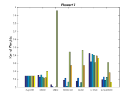
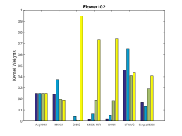
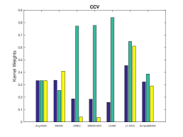
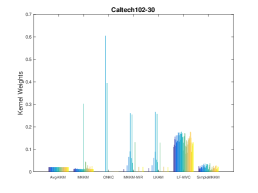
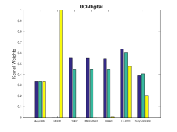
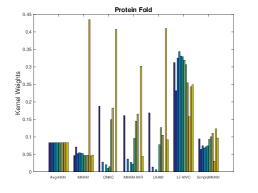
Figure 1: The kernel weights learned by different algorithms. SimpleMKKM maintains reduced sparsity compared to several competitors. Other datasets omitted due to space limit.

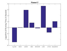
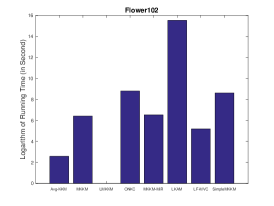
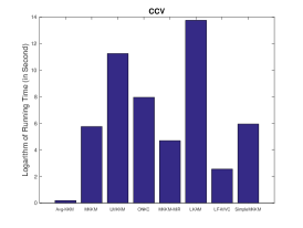
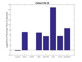
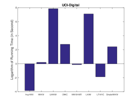
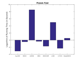
Figure 2: Run time of different algorithms on six benchmark datasets (in seconds). The experiments are conducted on a PC with Intel(R) Core(TM)-i7-5820 3.3 GHz CPU and 32G RAM in MATLAB environment. SimpleMKKM is comparably fast to alternatives while providing superior performance and requiring no hyper-parameter tuning. Results for other datasets are omitted due to space limit.

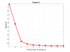
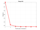
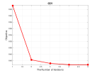
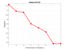
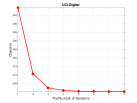
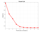
Figure 3: The objective of SimpleMKKM decreases with iterations. The curves for other datasets are omitted due to space limit.

For all algorithms, we repeat each experiment $50$ times with random initialization to reduce the effect of randomness caused by $k$-means, and report the means and variation. We next thoroughly study SimpleMKKM in terms of: clustering performance, the learned kernel weights, running time and algorithm convergence.

Along with SimpleMKKM, we ran another eight comparative algorithms in recent MKC literature, including

• Average kernel $k$-means (Avg-KKM). The consensus kernel is the uniformly combined base kernels, which is taken as the input of kernel $k$-means.

• Multiple kernel $k$-means (MKKM) (Huang et al., 2012). The base kernels are linearly combined into the consensus kernel. In addition, the combination weights are optimized along with clustering.

• Localized multiple kernel $k$-means(LMKKM) (Gönen & Margolin, 2014). The base kernels are combined with sample-adaptive weights.

• Optimal neighborhood kernel clustering (ONKC) (Liu et al., 2017b). The consensus kernel is chosen from the neighbor of linearly combined base kernels.

• Multiple kernel $k$-meanswith matrix-induced regularization (MKKM-MiR) (Liu et al., 2016b). The optimal combination weights are learned by introducing a matrix-induced regularization term to reduce the redundancy among the base kernels.

• Mulitple kernel clustering with local alignment maximization (LKAM) (Li et al., 2016). The similarity of a sample to its $k$-nearest neighbors, instead of all samples, is aligned with the ideal similarity matrix.

• Multi-view clustering via late fusion alignment maximization (LF-MVC) (Wang et al., 2019). Base partitions are first computed within corresponding data views and then integrated into a consensus partition.

• MKKM-MM (Bang et al., 2018). It proposes a $\min_{\mathbf{H}}$-$\max_{\boldsymbol{\gamma}}$ formulation that combines views in a way to reveal high within-cluster variance in the combined kernel space and then updates clusters by minimizing such variance.

The implementations of the above algorithms are publicly available in corresponding papers, and we directly adopt them without revision in our experiments. Among all the compared algorithms, ONKC (Liu et al., 2017b), MKKM-MiR (Liu et al., 2016b), LKAM (Li et al., 2016) and LF-MVC (Wang et al., 2019) have hyper-parameters to be tuned. We reuse their released Matlab codes and carefully tuned the hyper-parameters according to their setup to produce the best possible results on each dataset.

Table 3: Empirical comparison of SimpleMKKM with KAMM-R and KAMM-A on Flower17.

Dataset	KAMM-R	KAMM-A	SimpleMKKM
ACC	35.0$\pm$ 0.4	54.1$\pm$ 1.8	58.9$\pm$ 1.3
NMI	37.6$\pm$ 0.3	54.1$\pm$ 1.4	57.3$\pm$ 0.8
Purity	36.6 $\pm$ 0.5	55.1$\pm$ 1.8	60.2$\pm$ 1.4

5.2 Experimental Results

Clustering Performance

Table 2 presents the ACC, NMI and purity comparison of the above algorithms. From this table, we have the following observations:

• The proposed SimpleMKKM consistently and significantly outperforms MKKM. For example, it exceeds MKKM by $12.7\%,\,16\%,\,6.1\%,\,3.1\%,\,34.6\%,\,4.4\%,\,7.2\%,\,8.9\%,$
  $10.1\%,\,10.6\%$ and $11.7\%$ in terms of ACC on all benchmark datasets. These results demonstrate the efficacy of its min-max formulation and associated optimization algorithm.

• MKKM-MM (Bang et al., 2018) is the first try in literature to improve MKKM via minimization-maximization. As observed, it does improve the MKKM. However the improvement over MKKM is marginal on all datasets. Meanwhile, the proposed SimpleMKKM significantly outperforms MKKM-MM. This once again demonstrates the advantage of our formulation and the associated optimization strategy.

• Our SimpleMKKM achieves comparable or slightly better performance than MKKM-MiR (Liu et al., 2016b), ONKC (Liu et al., 2017b), and LF-MVC (Wang et al., 2019), all of which are considered the state of the art in multi-kernel clustering. Note that all of these algorithms have several hyper-parameters to tune due to the incorporation of regularization on the kernel weight $\boldsymbol{\gamma}$. Though demonstrating promising clustering performance, these algorithms need to take a lot of effort to determine the best hyper-parameters in practical applications. And parameter tuning may be impossible in real applications where there is no ground truth clustering to optimize. In contrast, our SimpleMKKM is parameter-free.

In summary, SimpleMKKM demonstrates superior clustering performance over the alternatives on all datasets and has no hyper-parameter to be tuned. We expect that the simplicity and efficacy of SimpleMKKM will make it a good option to be considered for practical clustering applications. Note that some results of LMKKM (Gönen & Margolin, 2014) are not reported due to out-of-memory errors, which are caused by its cubic computational and memory complexity.

Advantage of Formulation and Optimization

In order to show the advantage of the proposed formulation and optimization algorithm, we conduct an extra experiment on Flower17 to compare alternatives KAMM-R and KAMM-A. KAMM-R denotes optimizing kernel alignment $\mathrm{\mathbf{K}_{\boldsymbol{\gamma}\mathbf{H}\mathbf{H}^{\top}}}$ via maximizing $\boldsymbol{\gamma}$ and maximizing $\mathbf{H}$ with reduced gradient descent, and KAMM-A denotes optimizing this criterion via minimizing $\boldsymbol{\gamma}$ and maximizing $\mathbf{H}$ with alternate optimization (see Section 3.1 for discussion). KAMM-A has the same objective as SimpleMKKM, but it uses the widely adopted alternate optimization to solve it in place of our newly derived reduced gradient algorithm. From the results reported in Table 3, we clearly observe that: (1) Our SimpleMKKM formulation has significant advantage over KAMM-R, demonstrating the value of our novel min-max objective; (2) It also outperforms KAMM-A, which confirms that our new gradient-based optimization algorithm is also much better than the widely used alternate optimization.

Kernel Weight Analysis

We next investigate the kernel weights learned by the compared algorithms. The results are plotted in Figure 1. We can see that the kernel weights learned by MKKM are extremely sparse on some datasets such as UCI-Digital, which is caused by the alternate optimization. This sparsity insufficiently exploits the multiple kernel matrices and explains the weak performance of MKKM. For example, the clustering accuracy of MKKM on UCI-Digital is only $47.2\%$. However, despite the $\ell_{1}$-norm constraint on $\boldsymbol{\gamma}$, the kernel weights learned by our SimpleMKKM are all non-sparse on all datasets, which contributes to its superior clustering performance. This non-sparsity of the learned kernel weights is attributed to our new reduced gradient descent algorithm, which in turn is derived based on our new min-max kernel alignment objective.

Runtime and Convergence

We also report the running time of the compared algorithms in Figure 2. As observed, in addition to significantly improving performance, SimpleMKKM does not considerably increase the running time compared with MKKM and its variants. The objective of SimpleMKKM with iterations is reported in Figure 3. From these figures, we observe that the objective is monotonically decreased and the algorithm usually converges in less than ten iterations on all datasets. This corroborates our earlier theoretical analysis of the nature of our proposed objective and efficient optimisation algorithm.

6 Conclusion

In this paper, we have extended the widely used supervised kernel alignment criterion to clustering, and introduce a novel clustering objective of by minimizing alignment for $\boldsymbol{\gamma}$ and maximizing it for $\mathbf{H}$. We show that this novel objective can be transformed into a minimization problem which is differentiable and amenable to a solution by reduced gradient descent. This makes SimpleMKKM unique among MKC alternatives, in not requiring a local-minimum prone alternating coordinate descent strategy.

We derive a generalization bound for our approach using global Rademacher complexity analysis. Comprehensive experiments demonstrate the effectiveness of SimpleMKKM. We expect that the simplicity, lack of hyper-parameters, and efficacy of SimpleMKKM will make it a go-to solution for practical multi-kernel clustering applications in future. Future work may aim to extend SimpleMKKM to handle incomplete kernels, study further applications, and derive convergence rates using local Rademacher complexity analysis (Kloft & Blanchard, 2012; Cortes et al., 2013).

References

- Bang et al. (2018) Bang, S., Yu, Y., and Wu, W. Robust multiple kernel k-means clustering using min-max optimization, 2018.
- Bonnans & Shapiro (1998) Bonnans, J. F. and Shapiro, A. Optimization problems with perturbations: A guided tour. SIAM Review, 40(2):228–264, 1998.
- Chapelle et al. (2002) Chapelle, O., Vapnik, V., Bousquet, O., and Mukherjee, S. Choosing multiple parameters for support vector machines. Machine Learning, 46(1):131–159, Jan 2002.
- Cortes et al. (2009) Cortes, C., Mohri, M., and Rostamizadeh, A. L2 regularization for learning kernels. In UAI, pp. 109–116, 2009.
- Cortes et al. (2012) Cortes, C., Mohri, M., and Rostamizadeh, A. Algorithms for learning kernels based on centered alignment. JMLR, 13:795–828, 2012.
- Cortes et al. (2013) Cortes, C., Kloft, M., and Mohri, M. Learning kernels using local rademacher complexity. In Advances in Neural Information Processing Systems, pp. 2760–2768, 2013.
- Cristianini et al. (2002) Cristianini, N., Shawe-Taylor, J., Elisseeff, A., and Kandola, J. S. On kernel-target alignment. In Advances in Neural Information Processing Systems 14. 2002.
- Gönen & Margolin (2014) Gönen, M. and Margolin, A. A. Localized data fusion for kernel k-means clustering with application to cancer biology. In Advances in Neural Information Processing Systems 27: Annual Conference on Neural Information Processing Systems 2014, December 8-13 2014, Montreal, Quebec, Canada, pp. 1305–1313, 2014.
- Huang et al. (2012) Huang, H., Chuang, Y., and Chen, C. Multiple kernel fuzzy clustering. IEEE Trans. Fuzzy Systems, 20(1):120–134, 2012.
- Kloft & Blanchard (2012) Kloft, M. and Blanchard, G. On the convergence rate of lp-norm multiple kernel learning. J. Mach. Learn. Res., 13:2465–2502, 2012.
- Kloft et al. (2011) Kloft, M., Brefeld, U., Sonnenburg, S., and Zien, A. l-norm multiple kernel learning. JMLR, 12:953–997, 2011.
- Kumar & Daumé (2011) Kumar, A. and Daumé, H. A co-training approach for multi-view spectral clustering. In ICML, pp. 393–400, 2011.
- Kumar et al. (2011) Kumar, A., Rai, P., and Daumé, H. Co-regularized multi-view spectral clustering. In NIPS, pp. 1413–1421, 2011.
- Li et al. (2016) Li, M., Liu, X., Wang, L., Dou, Y., Yin, J., and Zhu, E. Multiple kernel clustering with local kernel alignment maximization. In Proceedings of the Twenty-Fifth International Joint Conference on Artificial Intelligence, IJCAI 2016, New York, NY, USA, 9-15 July 2016, pp. 1704–1710, 2016.
- Liu et al. (2016a) Liu, T., Tao, D., and Xu, D. Dimensionality-dependent generalization bounds for -dimensional coding schemes. Neural computation, 28(10):2213–2249, 2016a.
- Liu et al. (2016b) Liu, X., Dou, Y., Yin, J., Wang, L., and Zhu, E. Multiple kernel k-means clustering with matrix-induced regularization. In Proceedings of the Thirtieth AAAI Conference on Artificial Intelligence, February 12-17, 2016, Phoenix, Arizona, USA, pp. 1888–1894, 2016b.
- Liu et al. (2017a) Liu, X., Li, M., Wang, L., Dou, Y., Yin, J., and Zhu, E. Multiple kernel k-means with incomplete kernels. In AAAI, pp. 2259–2265, 2017a.
- Liu et al. (2017b) Liu, X., Zhou, S., Wang, Y., Li, M., Dou, Y., Zhu, E., and Yin, J. Optimal neighborhood kernel clustering with multiple kernels. In Proceedings of the Thirty-First AAAI Conference on Artificial Intelligence, February 4-9, 2017, San Francisco, California, USA, pp. 2266–2272, 2017b.
- Liu et al. (2019) Liu, X., Zhu, X., Li, M., Wang, L., Zhu, E., Liu, T., Kloft, M., Shen, D., Yin, J., and Gao, W. Multiple kernel k-means with incomplete kernels. IEEE Transactions on Pattern Analysis and Machine Intelligence, pp. 1–1, 2019. ISSN 1939-3539.
- Maurer & Pontil (2010) Maurer, A. and Pontil, M. -dimensional coding schemes in Hilbert spaces. IEEE Transactions on Information Theory, 56(11):5839–5846, 2010.
- Peng et al. (2019) Peng, X., Huang, Z., Lv, J., Zhu, H., and Zhou, J. T. COMIC: multi-view clustering without parameter selection. In Proceedings of the 36th International Conference on Machine Learning, ICML, pp. 5092–5101, 2019.
- Rakotomamonjy et al. (2008) Rakotomamonjy, A., Bach, F. R., Canu, S., and Grandvalet, Y. Simplemkl. JMLR, 9:2491–2521, 2008.
- Wang et al. (2019) Wang, S., Liu, X., Zhu, E., Tang, C., Liu, J., Hu, J., Xia, J., and Yin, J. Multi-view clustering via late fusion alignment maximization. In Proceedings of the Twenty-Eighth International Joint Conference on Artificial Intelligence, IJCAI 2019, Macao, China, August 10-16, 2019, pp. 3778–3784, 2019.
- Yu et al. (2012) Yu, S., Tranchevent, L.-C., Liu, X., Glänzel, W., Suykens, J. A. K., Moor, B. D., and Moreau, Y. Optimized data fusion for kernel k-means clustering. IEEE TPAMI, 34(5):1031–1039, 2012.
- Zhao et al. (2009) Zhao, B., Kwok, J. T., and Zhang, C. Multiple kernel clustering. In SDM, pp. 638–649, 2009.