Topological characterization of one-dimensional open fermionic systems

Abstract

A topological measure characterizing symmetry-protected topological phases in one-dimensional open fermionic systems is proposed. It is built upon the kinematic approach to the geometric phase of mixed states and facilitates the extension of the notion of topological phases from zero-temperature to nonzero-temperature cases. In contrast to a previous finding that topological properties may not survive above a certain critical temperature, we find that topological properties of open systems, in the sense of the measure suggested here, can persist at any finite temperature and disappear only in the mathematical limit of infinite temperature. Our result is illustrated with two paradigmatic models of topological matter. The bulk topology at nonzero temperatures manifested as robust mixed edge state populations is examined via two figures of merit.

Berry phase is a fundamental concept in quantum physics, revealing a gauge field governing parallel transport (originally for pure states) Berry (1984). It was later realized that the Berry phase of electronic wave functions has a profound effect on topological properties of materials and is responsible for a number of topological phenomena Xiao et al. (2010). A seminal example is the integer quantum Hall effect, which is related to the Berry phase for a contour enclosing a two-dimensional Brillouin zone and determines the quantized value of the Hall conductivity of filled bands Thouless et al. (1982). Besides the integer quantum Hall effect, several fascinating discoveries in modern condensed-mater physics, including topological insulators and topological superconductors Hasan and Kane (2010); Qi and Zhang (2011), are also deeply connected to the Berry phase.

Any realistic quantum system at a nonzero temperature, however, inevitably interacts with its environment and is described by mixed states rather than pure states. This historically stimulated the development towards extending the Berry phase to the realm of mixed states. Uhlmann was the first to address the issue of mixed-state holonomy. He formulated a new parallel transport condition defining parallelity and holonomy for mixed states, with which the Uhlmann phase was put forward Uhlmann (1986, 1991, 1993). Another definition of the geometric phase for mixed states is proposed by Tong et al., based on a kinematic approach, without a priori assumption about the dynamics of open systems Tong et al. (2004). In addition, there have been other formulations of parallel transport conditions for mixed states and several alternative but nonequivalent definitions have been proposed accordingly Sjöqvist et al. (2000); Whitney and Gefen (2003); Ericsson et al. (2003); Filipp and Sjöqvist (2003); Carollo et al. (2003, 2004); Whitney et al. (2005).

Armed with the concept of geometric phase for mixed states, it becomes possible to investigate the role of thermal and dissipative effects in topological phases of matter. In particular, what is the impact of a nonzero temperature on the topological characterization of an otherwise topologically nontrivial system at zero temperature? This topic has received much attention recently Diehl et al. (2011); Rivas et al. (2013); Viyuela et al. (2014a, b); Huang and Arovas (2014); van Nieuwenburg and Huber (2014); Budich and Diehl (2015); Viyuela et al. (2015); Mera et al. (2017); Viyuela et al. (2018); He et al. (2018); Bardyn et al. (2018); Caldas et al. (2018); Paunković and Vieira (2018); Amin et al. ; Leonforte et al. , with the Uhlmann phase used as the main tool. Viyuela et al. introduced the Uhlmann phase as a topological measure for one-dimensional (1D) open fermionic systems Viyuela et al. (2014a). For physical models considered there, topological properties in the sense of their topological measure were found to disappear above a certain critical temperature, at which a certain Uhlmann phase goes discontinuously and abruptly to zero. Later on, similar results were found in two-dimensional open fermionic systems, with the aid of proper topological invariants constructed out of the Uhlmann phase Viyuela et al. (2014b); Huang and Arovas (2014). Although much progress has been made by use of the Uhlmann phase, it is just the beginning to study thermal topological behavior with respect to other legitimate definitions of mixed-state geometric phase. Indeed, to our best knowledge, attempts were made only for the interferometric phase Sjöqvist et al. (2000), and the associated calculations for the Kitaev chain Andersson et al. (2016); Bhattacharya and Dutta (2018) yield results different from those obtained from the Uhlmann phase approach. Despite the lack of extensive studies, the existing results already indicate that the physical picture of thermal topological phases of matter may not be fully captured by the Uhlmann phase, and therefore, more efforts concerning other definitions of mixed-state geometric phase are desirable.

In this paper, based on the kinematic approach to the geometric phase for mixed states Tong et al. (2004), we introduce a topological measure to characterize symmetry-protected topological phases in 1D open fermionic systems. It places the temperature under equal footing with other tuneable system parameters, thus providing a way for extending the notion of topological phases to cases with nonzero temperature. To reveal the physical implication of our topological measure, we further introduce two figures of merit, which can measure the degree of the presence of mixed edge states. As examples, we use our topological measure to identify the bulk topological invariants of two paradigmatic models of symmetry protected topological matter under arbitrary temperature. We also investigate the physical implication of the bulk topology for robust mixed edge states with the aid of our figures of merit. Although the derivation of our topological measure is relatively simple, it depicts an interesting physical picture of thermal topological phases different from that in the previous work Viyuela et al. (2014a).

To present our finding clearly, we need first to recapitulate the kinematic approach to the geometric phase for mixed states. Consider an open quantum system $s$ equipped with a $N$ dimensional Hilbert space $\mathcal{H}_{s}$. An evolution of the state of $s$ can be expressed as the path

$$\mathcal{P}:t\in[0,\tau]\mapsto\rho(t)=\sum_{j=1}^{N}p_{j}(t)|\phi_{j}(t)\rangle\langle\phi_{j}(t)|,$$ (1)

where $p_{j}(t)$ and $|\phi_{j}(t)\rangle$ are the eigenvalues and eigenvectors of the density operator $\rho(t)$, respectively. In order to associate the path $\mathcal{P}$ with a geometric phase, the mixed state in the path is lifted to a pure state by the standard purification procedure,

$$|\Phi(t)\rangle=\sum_{j=1}^{N}\sqrt{p_{j}(t)}|\phi_{j}(t)\rangle\otimes|a_{j}\rangle,$$ (2)

where an auxiliary quantum system $a$ is introduced, and $|a_{j}\rangle$ denotes a fixed orthonormal basis of its Hilbert space $\mathcal{H}_{a}$. Note that there is redundancy in the expression (2), because of the gauge degree of freedom in choosing states $|\phi_{j}(t)\rangle$. If all the nonzero $p_{j}(t)$ are non-degenerate during the evolution, the redundancy in Eq. (2) can be removed by imposing the following parallel transport condition on $|\phi_{j}(t)\rangle$,

$$\langle\phi_{j}(t)|\partial_{t}|\phi_{j}(t)\rangle=0,~{}~{}~{}~{}j=1,\dots,N.$$ (3)

Under the condition of Eq. (3), the state $|\Phi(t)\rangle$ experiences the Berry-Simon parallel transport, i.e., $\langle\Phi(t)|\partial_{t}|\Phi(t)\rangle=0$ Berry (1984); Simon (1983). The acquired relative phase between $|\Phi(\tau)\rangle$ and $|\Phi(0)\rangle$ is defined to be the geometric phase associated with the path $\mathcal{P}$, namely, $\gamma[\mathcal{P}]:=\arg\langle\Phi(0)|\Phi(\tau)\rangle$. Substituting Eq. (2) into this defining expression yields

$$\gamma[\mathcal{P}]=\arg\left(\sum_{j=1}^{N}\sqrt{p_{j}(0)p_{j}(\tau)}\langle\phi_{j}^{\shortparallel}(0)|\phi_{j}^{\shortparallel}(\tau)\rangle\right),$$ (4)

with $|\phi_{j}^{\shortparallel}(t)\rangle$ satisfying Eq. (3). Here, to indicate the fact that the eigenvectors undergo parallel transport, i.e., satisfy Eq. (3), we use $|\phi_{j}^{\shortparallel}(t)\rangle$ instead of $|\phi_{j}(t)\rangle$ to represent it. Moreover, a gauge-invariant expression for $\gamma[\mathcal{P}]$ reads

$$\gamma[\mathcal{P}]=\arg\left(\sum_{j=1}^{N}\sqrt{p_{j}(0)p_{j}(\tau)}\langle\phi_{j}(0)|\phi_{j}(\tau)\rangle e^{-\int_{0}^{\tau}\langle\phi_{j}(t)|\partial_{t}|\phi_{j}(t)\rangle\mathrm{d}t}\right),$$ (5)

where $|\phi_{j}(t)\rangle$ is not necessary to fulfill Eq. (3). The invariance of Eq. (5) under gauge transformations $|\phi_{j}(t)\rangle\mapsto e^{i\theta_{j}(t)}|\phi_{j}(t)\rangle$, $\theta_{j}(t)$ real, can be checked straightforwardly. In the case that some of the nonzero $p_{j}(t)$ are degenerate, the path $\mathcal{P}$ may be rewritten as

$$\mathcal{P}:t\in[0,\tau]\mapsto\rho(t)=\sum_{j=1}^{K}\sum_{\mu=1}^{n_{j}}p_{j}(t)|\phi_{j}^{\mu}(t)\rangle\langle\phi_{j}^{\mu}(t)|,$$ (6)

where $p_{j}(t)$, $j=1,\dots,K$, are the eigenvalues of $\rho(t)$ with degeneracy $n_{j}$, and $|\phi_{j}^{\mu}(t)\rangle$, $\mu=1,\dots,n_{j}$, are the corresponding degenerate eigenvectors. In this case, the parallel transport condition in Eq. (3) is no longer capable of completely removing the redundancy in the standard purification procedure. As a consequence, it should be replaced by

$$\langle\phi_{j}^{\mu}(t)|\partial_{t}|\phi_{j}^{\nu}(t)\rangle=0,~{}~{}~{}~{}\mu,\nu=1,\dots,n_{j},$$ (7)

while the remainder of the process of defining $\gamma[\mathcal{P}]$ is unchanged.

With the above knowledge, we now move on to our topic of introducing a topological measure for 1D open fermionic systems.

For simplicity, we consider a two-band single-particle model describing a topological insulator. Under periodic boundary condition, the Hamiltonian of the model can be generally expressed as

$$H=\sum_{k}\psi^{\dagger}(k)H(k)\psi(k),$$ (8)

where $H(k):=d_{0}(k)+\sum_{i=1}^{3}d_{i}(k)\sigma_{i}$ is the bulk momentum-space Hamiltonian and $\psi(k):=(a_{k},b_{k})^{t}$ stands for the spinor representation, with $\sigma_{i}$ denoting the Pauli matrices and $a_{k}$, $b_{k}$ representing two species of fermionic annihilation operators. Our discussion below can be easily generalized to models of superconductors by using the Nambu spinor Altland and Simons (2010) instead.

When a non-vanishing gap exists in the energy spectrum of $H(k)$, the vector $\bm{d}(k):=(d_{1}(k),d_{2}(k),d_{3}(k))$ is non-zero for all $k$, and its normalized vector $\hat{\bm{d}}(k):=\bm{d}(k)/\lvert\bm{d}(k)\rvert$ defines a mapping from the Brillouin zone into the unit sphere $S^{2}$. This mapping is, however, topologically trivial, as the first homotopy group of $S^{2}$ is trivial. Hence, symmetry is needed, in order to put further constraints on $\hat{\bm{d}}(k)$ and induce a non-trivial topology. For 1D fermionic systems, the symmetry needed is typically the chiral symmetry, i.e., a unitary matrix $\Gamma$ satisfying $\Gamma^{2}=1$ and $\Gamma H(k)\Gamma=-H(k)$ Altland and R. Zirnbauer (1997); Ryu et al. (2010); Chiu et al. (2016).

Under the natural assumption of the system being in thermodynamic equilibrium with a reservoir, its state is given by the grand canonical ensemble, $\rho=\frac{1}{Z}e^{-\beta(H-\mu N)}$, where $Z$ is the partition function, $N$ the total number operator, $\mu$ the chemical potential, and $\beta:=\frac{1}{k_{b}T}$ the reciprocal of the temperature $T$, with $k_{b}$ being the Boltzmann’s constant. Here we have assumed that there are no interactions when two or more particles are present in the system. Note also that it is possible (but not always) for the grand canonical ensemble to emerge as the unique steady state from the Lindbladian dynamics Rivas et al. (2013). In the single-particle picture, the state of the system is described by the one-body density matrix Cheong and L. Henley (2004)

$$\rho(k)=\sum_{j=\pm}\omega_{j}(k)|\mu_{j}(k)\rangle\langle\mu_{j}(k)|,$$ (9)

where $|\mu_{j}(k)\rangle$, $j=\pm$, are the eigenvectors of $H(k)$, i.e., $H(k)|\mu_{j}(k)\rangle=\varepsilon_{j}(k)|\mu_{j}(k)\rangle$, and $\omega_{j}(k)$ are the Fermi weights expressed as $\omega_{j}(k)=1/[e^{\beta(\varepsilon_{j}(k)-\mu)}+1]$.

To arrive at our topological measure, we need to discuss the geometric phase associated with the path

$$\mathcal{P}:k\in[-\pi,\pi]\mapsto\rho(k)$$ (10)

case by case. Here, in the spirit of Zak’s phase Zak (1989), the Bloch quasimomentum $k$ plays the role of $t$ appearing in Eq. (1). Consider first the case of arbitrary $\beta>0$ and $\varepsilon_{-}(k)\neq\varepsilon_{+}(k)$ for all $k$, i.e., any finite temperature and non-vanishing bulk gap. Adopting a cyclic gauge, i.e., $|\mu_{j}(-\pi)\rangle=|\mu_{j}(\pi)\rangle$, we have that the Berry phase associated with $|\mu_{j}(k)\rangle$ reads $\gamma_{j}=i\int_{-\pi}^{\pi}\mathrm{d}k\langle\mu_{j}(k)|\partial_{k}|\mu_{j}(k)\rangle$. Substituting $\omega_{j}(k)$ and $|\mu_{j}(k)\rangle$ into Eq. (5) and using the equalities $\omega_{j}(-\pi)=\omega_{j}(\pi)$ and $|\mu_{j}(-\pi)\rangle=|\mu_{j}(\pi)\rangle$, we have

$$\gamma[\mathcal{P}]=\arg[\omega_{-}(\pi)e^{i\gamma_{-}}+\omega_{+}(\pi)e^{i\gamma_{+}}].$$ (11)

On the other hand, by representing $\Gamma$ in the form $\Gamma=\bm{n}\cdot\bm{\sigma}$ with $\bm{n}$ a constant vector of unit length, the chiral symmetry condition $\Gamma H(k)\Gamma=-H(k)$ gives $\bm{n}\cdot\bm{d}(k)=0$. It follows that $\bm{d}(k)$ is restricted to the plane perpendicular to $\bm{n}$, and $\hat{\bm{d}}(k)$ now defines a mapping from the Brillouin zone into the circle $S^{1}$. The topology of such a mapping is characterized by the winding number, $\nu=\frac{1}{2\pi}\int_{-\pi}^{\pi}\mathrm{d}k[\hat{\bm{d}}(k)\times\partial_{k}\hat{\bm{d}}(k)]\cdot\bm{n}$, counting the number of times that $\hat{\bm{d}}(k)$ travels around the origin as $k$ goes through the Brillouin zone. It is not difficult to see that the relationship between the Berry phase and the winding number is $\gamma_{-}=-\gamma_{+}=\pi\nu$ up to an integer multiple of $2\pi$. Substituting this equality into Eq. (11) and simplifying the resultant equation by using $\omega_{j}(\pi)>0$, we obtain

$$\gamma[\mathcal{P}]=\arg[\cos(\pi\nu)].$$ (12)

Consider next the case of $\beta=0$, i.e., infinite temperature, which is mathematically allowed but not so physical. Here, the spectrum $\varepsilon_{j}(k)$ may be gapped or gapless. In this case, all the $\omega_{j}(k)$ in Eq. (9) equals $1/2$ and hence $\mathcal{P}:k\in[-\pi,\pi]\mapsto\rho(k)$ represents a path with degeneracy. Therefore, we need to find the eigenvectors $|\mu_{j}(k)\rangle$ of $\rho(k)$ that satisfy Eq. (7). Without loss of generality, $|\mu_{j}(k)\rangle$ can be chosen as $|\mu_{-}(k)\rangle=(1,0)^{t}$ and $|\mu_{+}(k)\rangle=(0,1)^{t}$. Inserting the two expressions into Eq. (4) yields

$$\gamma[\mathcal{P}]=0.$$ (13)

Finally, for the last case of $\beta>0$ and $\varepsilon_{-}(k)=\varepsilon_{+}(k)$ for some $k$, i.e., an arbitrary finite temperature but with a gapless spectrum, there may exist gauges $|\mu_{j}(k)\rangle$ such that $\langle\mu_{j}(-\pi)|\mu_{j}(\pi)\rangle=0$, $j=\pm$ not . From Eq. (5), it follows immediately that $\gamma[\mathcal{P}]=\arg 0$, indicating that $\gamma[\mathcal{P}]$ is ill-defined in general. Now, combining the three cases, we obtain the topological measure:

$$\gamma[\mathcal{P}]=(1-\delta_{\beta,0})\arg[\cos(\pi\nu)],$$ (14)

which is defined for the case of arbitrary finite temperature but with gapped spectrum or for the case of arbitrary spectrum but with the infinite temperature.

It is worth noting that several conditions have been speculated to be necessary for a functional to be a legitimate topological measure in the setting considered here Rivas et al. (2013); Viyuela et al. (2014a); Huang and Arovas (2014). (i) In the limit of zero temperature, it should reduce to usual topological order parameters, e.g., the Berry phase. (ii) It should not increase in the course of increasing temperature, i.e., topological order cannot be created by temperature. (iii) In the limit of infinite temperature, it should be zero, i.e., topological order must be spoiled completely. It can be verified our measure proposed in Eq. (14) fulfills all the conditions. Besides, it is also worth comparing the derivation presented here with that in Ref. Viyuela et al. (2014a). Both the derivation here and that in Ref. Viyuela et al. (2014a) are on the basis of purifications of mixed states. The purification in Ref. Viyuela et al. (2014a) is to express $\rho(t)$ as $\rho(t)=w(t)w^{\dagger}(t)$, with $w(t)$ being an operator. In contrast, the procedure involved here is given by Eq. (2), which aims to express $\rho(t)$ as a superposition of pure states via an auxiliary quantum system. Therefore, by construction, our topological measure is distinct from the method proposed in Ref. Viyuela et al. (2014a). As far as we can see, there is no reason to prefer one kind of purification of mixed states but abandon the other, which is one of the motivations of this paper.

Our topological measure is very simple. For any finite temperature, if $\nu=0$ then $\gamma[\mathcal{P}]=0$; and if $\nu=1$ then $\gamma[\mathcal{P}]=\pi$. Only for the limit of infinite temperature (i.e., $\beta=0$), $\gamma[\mathcal{P}]=0$, regardless of whether the zero-temperature phase is topologically trivial or nontrivial. Despite the simplicity of our measure, it produces some interesting implications for the population of mixed edge states. Before showing this, let us first elaborate on the topological characterization of two paradigmatic models using our measure.

Example 1: SSH model.—The Su-Schrieffer-Heeger (SSH) model describes spin-polarized electrons hopping on a dimerized chain Su et al. (1979); Rice and Mele (1982). In the language of Altland-Zirnbauer classification Altland and R. Zirnbauer (1997); Ryu et al. (2010); Chiu et al. (2016), it belongs to the BDI class. The Hamiltonian of the model reads

$$H_{\textrm{SSH}}=\sum_{j=1}^{L}(J+\alpha)a_{j}^{\dagger}b_{j}+(J-\alpha)a_{j}^{\dagger}b_{j-1}+\textrm{H.c.},$$ (15)

where $a_{j}$ and $b_{j}$ are the fermionic annihilation operators acting on the $j$-th unit cell which hosts two sites, one on sublattice $A$ and the other on sublattice $B$. $J+\alpha\geq 0$ and $J-\alpha\geq 0$ denote the intracell and intercell hopping amplitudes, respectively, with $\alpha$ characterizing the imbalance between them. Hereafter, we set $J=1$. It is known that $\nu=1$ for $\alpha<0$ and $\nu=0$ for $\alpha>0$. From this, it follows that $\gamma[\mathcal{P}]=\pi$ for $\alpha<0$ and $\beta>0$, corresponding to the topologically non-trivial region, and $\gamma[\mathcal{P}]=0$ for $\alpha>0$ and $\beta>0$ or $\beta=0$, corresponding to the topologically trivial region.

Example 2: Creutz ladder.—The Creutz ladder (CL) model describes spin-polarized electrons moving in a ladder system Creutz (1999); Bermudez et al. (2009). It belongs to the AIII class. The Hamiltonian of the model reads

$$H_{\textrm{CL}}= - \sum_{j=1}^{L}[K(e^{-i\theta}a_{j+1}^{\dagger}a_{j}+e^{i\theta}b_{j+1}^{\dagger}b_{j})$$ (16)

$$+ K(b_{j+1}^{\dagger}a_{j}+a_{j+1}^{\dagger}b_{j})+Ma_{j}^{\dagger}b_{j}+\textrm{H.c.}],$$

where $a_{j}$ and $b_{j}$ are the fermionic annihilation operators acting on the $j$-th sites of the upper and lower chain, respectively. The hopping along horizontal and diagonal links is described by the parameter $K$, and the vertical one by $M$. Additionally, a magnetic flux $\theta\in[-\pi/2,\pi/2]$ is induced by a perpendicular magnetic field. Hereafter, we set $K=1$, $\theta=\pi/2$, and redefine a new parameter $\alpha:=-1+\frac{M}{2K}$. It is known that $\nu=1$ for $\alpha<0$ and $\nu=0$ for $\alpha>0$. From this, it follows that $\gamma[\mathcal{P}]=\pi$ for $\alpha<0$ and $\beta>0$, corresponding to the topologically non-trivial region, and $\gamma[\mathcal{P}]=0$ for $\alpha>0$ and $\beta>0$ or $\beta=0$, corresponding to the topologically trivial region.

A remarkable manifestation of nontrivial bulk topology is the emergence of edge states. For zero-temperature cases this is known as the bulk-boundary correspondence. Can this physical picture carry over to cases with non-zero temperature? After introducing our topological measure, it is natural to examine the equilibrium profiles of edge states associated with topologically distinct regions identified by the measure.

To answer the above question, we need a figure of merit to characterize the distinguishability between mixed edge states and bulk states. Such a figure of merit should be a function of the system parameters and the temperature. For the models considered throughout this paper, one key system parameter is $\alpha$ for both models albeit carrying different meanings, and for this reason we shall denote the figure of merit as $\Lambda(\alpha,\beta)$. Let us assume that $\Lambda(\alpha,\beta)$ is defined as

$$\Lambda(\alpha,\beta):=\lvert\langle\overline{N}_{\textrm{edge}}\rangle_{\rho}-\langle\overline{N}_{\textrm{bulk}}\rangle_{\rho}\rvert,$$ (17)

leaving the discussion on alternative definition for $\Lambda(\alpha,\beta)$ to the end of this paper. Here, $\langle O\rangle_{\rho}=\mathrm{Tr}(O\rho)$ stands for expectation values of observables $O$, and $\rho$ is again the grand canonical ensemble, i.e., $\rho=\frac{1}{Z}e^{-\beta(H-\mu N)}$, with $H$ being any one of the Hamiltonians in Eqs. (15) and (16) under open boundary conditions. The two observables in Eq. (17) are defined as $\overline{N}_{\textrm{edge}}:=\sum_{i\in I_{e}}N_{i}/\lvert I_{e}\rvert$ and $\overline{N}_{\textrm{bulk}}:=\sum_{i\in I_{b}}N_{i}/\lvert I_{b}\rvert$, where $N_{i}$ is the particle number operator, and $I_{e}$ and $I_{b}$ denote the index sets for the edge and bulk, respectively. For the SSH model, $I_{e}$ is comprised of the site of the first unit cell on sublattice $A$ and that of the last unit cell on sublattice $B$, while for the CL model, $I_{e}$ is comprised of the first sites of the upper and lower chain and the last sites of the upper and lower chain. $I_{b}$ is the complementary set of $I_{e}$. The two expectation values $\langle\overline{N}_{\textrm{edge}}\rangle_{\rho}$ and $\langle\overline{N}_{\textrm{bulk}}\rangle_{\rho}$ by their very nature represent the average particle occupation numbers in the edge and bulk, respectively. Roughly speaking, a non-negligible value of the figure of merit implies that the average particle occupation number in the edge is distinguishable from that in the bulk. This indicates the presence of mixed edge states. By contrast, a negligible value of our figure of merit represents that the average particle occupation number in the edge is barely distinguishable from that in the bulk, thus indicating the absence of mixed edge states.

With the figure of merit in Eq. (17), we now study the profiles of edge states of the two models, with respect to different topological regions identified by our measure. Henceforth, we set the chemical potential $\mu=0.1$ without loss of generality.

Consider first the SSH model. For the flat-band case, i.e., $\alpha=\pm 1$, we analytically calculate the figure of merit in Eq. (17). After some algebra, it is found that

$$\Lambda(-1,\beta)=\frac{1}{e^{-\beta\mu}+1}- \frac{1}{2}\left[\frac{1}{e^{-\beta(\mu-2)}+1}+\frac{1}{e^{-\beta(\mu+2)+1}}\right],$$

with $(\alpha,\beta)=(-1,\beta)$ belonging to the topologically non-trivial region for $\beta>0$ and the topologically trivial region for $\beta=0$, and

$$\Lambda(1,\beta)=0,$$ (19)

with $(\alpha,\beta)=(1,\beta)$ belonging to the topologically trivial region for all $\beta\geq 0$. Note that $\Lambda(\alpha,\beta)>0$ indicates the presence of edge states while $\Lambda(\alpha,\beta)=0$ implies the absence of edge states, and also note that $\Lambda(-1,\beta)>0$ when $\beta>0$ and $\Lambda(-1,\beta)=0$ when $\beta=0$. From Eqs. (Topological characterization of one-dimensional open fermionic systems) and (19), it follows immediately that edge states are present in the topologically non-trivial region while absent in the topologically trivial region.

For the general case, analytical solutions may be difficult to obtain and we resort to numerical computation. Figure 1 shows $\Lambda(\alpha,\beta)$ for the parameters given in the figure caption.

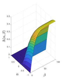
Figure 1: Figure of merit for the SSH model. Parameters used are: $L=100$, $J=1$, and $\mu=0.1$.

According to whether the value of $\Lambda(\alpha,\beta)$ is negligible or not, we can divide the domain of $\Lambda(\alpha,\beta)$ into two regions. As can be seen in Fig. 1, the region associated with negligible values of $\Lambda(\alpha,\beta)$, referred to as the negligible region for convenience, is $\alpha>0$ and $\beta>0$ or $\beta=0$, and the region associated with non-negligible values of $\Lambda(\alpha,\beta)$, referred to as the non-negligible region, is $\alpha<0$ and $\beta>0$. The negligible and non-negligible regions are identical with the topologically trivial and non-trivial regions identified by our measure, respectively. Note that non-negligible (negligible) values of the figure of merit indicate the presence (absence) of edge states. It implies that edge states are present in the topologically non-trivial region while absent in the topologically trivial region for the SSH model. The results here strongly support our use of the figure of merit and the physical relevance of our topological characterization.

Consider now the CL model. For the flat-band case, we obtain the same analytical result as that of the SSH model. For the general case, we resort to numerical computation. The numerical result is shown in Fig. 2, for the

Figure 2: Figure of merit for the CL model. Parameters used are: $L=100$, $K=1$, and $\mu=0.1$.

parameters given in the figure caption. Again, we divide the domain of $\Lambda(\alpha,\beta)$ into two regions, according to whether the value of $\Lambda(\alpha,\beta)$ is negligible or not. From Fig. 2, we deduce that the negligible region is $\alpha>0$ and $\beta>0$ or $\beta=0$, being identical with the topologically trivial region, and the non-negligible region is $\alpha<0$ and $\beta>0$, being identical with the topologically non-trivial region. It indicates that edge states are present in the topologically non-trivial region while absent in the topologically trivial region for the CL model, too.

Besides, we have numerically examined the robustness of edge states by adding disorder to the Hamiltonians in Eqs. (15) and (16). The numerical results show that the presence of edge states is insensitive to moderate disorder.

Before concluding, we discuss briefly some aspects of alternative definition of the figure of merit. In the foregoing paragraphs, we have adopted, perhaps, the simplest definition for $\Lambda(\alpha,\beta)$. To characterize the distinguishability between mixed edge and bulk states, one may alternatively adopt the following definition:

$$\Lambda(\alpha,\beta):=\min_{i\in I_{e};j\in I_{b}}\lvert\langle N_{i}\rangle_{\rho}-\langle N_{j}\rangle_{\rho}\rvert,$$ (20)

representing the distance between the occupation numbers of electrons in the edge and those in the bulk. It can be shown that the negligible and non-negligible regions with Eq. (20) are in agreement with the corresponding ones with Eq. (17), respectively (for the details, see Appendix). As an immediate consequence, our statements on the bulk-boundary correspondence in the previous paragraphs hold true for the alternative definition in Eq. (20), too.

In conclusion, we have suggested an alternative and simple measure for characterizing symmetry-protected topological phases in 1D open chiral fermionic systems. It places the temperature under equal footing with other system parameters, thus extending the notion of topological phases from zero-temperature to nonzero-temperature cases. As examples of its application, we have used our method to identify the bulk topology of two paradigmatic models of topological matter.

In revealing the physical implication of our simple topological characterization, we have introduced two figures of merit, which indicate the presence of mixed edge states when its value is non-negligible. With them we have shown that mixed edge states are present in the topologically non-trivial region while absent in the topologically trivial region for the two models. We hence conclude that bulk-edge correspondence does hold under our measure, at arbitrary finite temperatures.

Interestingly, in contrast to the Uhlmann construction Viyuela et al. (2014a), for which topological properties cannot survive above a certain critical temperature, we find that topological properties in the sense of our measure can persist at any finite temperature but disappear in the limit of infinite temperature. Moreover, with our measure the bulk-edge correspondence still holds, whereas it does not exist using the topological invariants under the Uhlmann construction. Our findings are in agreement with the observation made for quasi-local dissipative dynamics in Refs. Diehl et al. (2011); Bardyn et al. (2013), where a topological invariant was formulated in terms of chirally symmetric density matrices and a dissipative bulk-edge correspondence was established. Finally, we would like to point out that our measure may be experimentally measured with a NMR quantum simulator Cucchietti et al. (2010).

appendix

In this Appendix, we identify the negligible and non-negligible regions of the SSH model and the CL model, with the aid of the alternative definition in Eq. (20). For the SSH model, the numerical result is shown in Fig. 3.

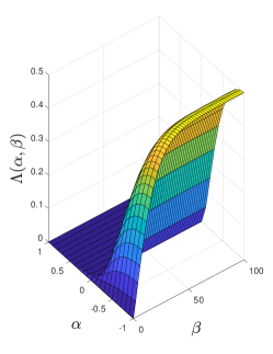
Figure 3: Figure of merit for the SSH model with the alternative expression in Eq. (20). Parameters used are: $L=100$, $J=1$, and $\mu=0.1$.

As can be seen in Fig. 3, the negligible region is $\alpha>0$ and $\beta>0$ or $\beta=0$, and the non- negligible region is $\alpha<0$ and $\beta>0$. For the CL model, the numerical result is shown in Fig. 4.

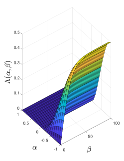
Figure 4: Figure of merit for the CL model with the alternative expression in Eq. (20). Parameters used are: $L=100$, $K=1$, and $\mu=0.1$.

As can be seen in Fig. 4, the negligible region is $\alpha>0$ and $\beta>0$ or $\beta=0$, and the non-negligible region is $\alpha<0$ and $\beta>0$.

References

- Berry (1984) M. V. Berry, Proc. R. Soc. Lond. A 392, 45 (1984).
- Xiao et al. (2010) D. Xiao, M.-C. Chang, and Q. Niu, Rev. Mod. Phys. 82, 1959 (2010).
- Thouless et al. (1982) D. J. Thouless, M. Kohmoto, M. P. Nightingale, and M. den Nijs, Phys. Rev. Lett. 49, 405 (1982).
- Hasan and Kane (2010) M. Z. Hasan and C. L. Kane, Rev. Mod. Phys. 82, 3045 (2010).
- Qi and Zhang (2011) X.-L. Qi and S.-C. Zhang, Rev. Mod. Phys. 83, 1057 (2011).
- Uhlmann (1986) A. Uhlmann, Rep. Math. Phys. 24, 229 (1986).
- Uhlmann (1991) A. Uhlmann, Lett. Math. Phys. 21, 229 (1991).
- Uhlmann (1993) A. Uhlmann, Rep. Math. Phys. 33, 253 (1993).
- Tong et al. (2004) D. M. Tong, E. Sjöqvist, L. C. Kwek, and C. H. Oh, Phys. Rev. Lett. 93, 080405 (2004).
- Sjöqvist et al. (2000) E. Sjöqvist, A. K. Pati, A. Ekert, J. S. Anandan, M. Ericsson, D. K. L. Oi, and V. Vedral, Phys. Rev. Lett. 85, 2845 (2000).
- Whitney and Gefen (2003) R. S. Whitney and Y. Gefen, Phys. Rev. Lett. 90, 190402 (2003).
- Ericsson et al. (2003) M. Ericsson, A. K. Pati, E. Sjöqvist, J. Brännlund, and D. K. L. Oi, Phys. Rev. Lett. 91, 090405 (2003).
- Filipp and Sjöqvist (2003) S. Filipp and E. Sjöqvist, Phys. Rev. Lett. 90, 050403 (2003).
- Carollo et al. (2003) A. Carollo, I. Fuentes-Guridi, M. F. Santos, and V. Vedral, Phys. Rev. Lett. 90, 160402 (2003).
- Carollo et al. (2004) A. Carollo, I. Fuentes-Guridi, M. F. Santos, and V. Vedral, Phys. Rev. Lett. 92, 020402 (2004).
- Whitney et al. (2005) R. S. Whitney, Y. Makhlin, A. Shnirman, and Y. Gefen, Phys. Rev. Lett. 94, 070407 (2005).
- Diehl et al. (2011) S. Diehl, E. Rico, M. A. Baranov, and P. Zoller, Nat. Phys. 7, 971 (2011).
- Rivas et al. (2013) A. Rivas, O. Viyuela, and M. A. Martin-Delgado, Phys. Rev. B 88, 155141 (2013).
- Viyuela et al. (2014a) O. Viyuela, A. Rivas, and M. A. Martin-Delgado, Phys. Rev. Lett. 112, 130401 (2014a).
- Viyuela et al. (2014b) O. Viyuela, A. Rivas, , and M. A. Martin-Delgado, Phys. Rev. Lett. 113, 076408 (2014b).
- Huang and Arovas (2014) Z. Huang and D. P. Arovas, Phys. Rev. Lett. 113, 076407 (2014).
- van Nieuwenburg and Huber (2014) E. P. L. van Nieuwenburg and S. D. Huber, Phys. Rev. B 90, 075141 (2014).
- Budich and Diehl (2015) J. C. Budich and S. Diehl, Phys. Rev. B 91, 165140 (2015).
- Viyuela et al. (2015) O. Viyuela, A. Rivas, and M. A. Martin-Delgado, 2D Mater. 2, 034006 (2015).
- Mera et al. (2017) B. Mera, C. Vlachou, N. Paunković, and V. R. Vieira, Phys. Rev. Lett. 119, 015702 (2017).
- Viyuela et al. (2018) O. Viyuela, A. Rivas, S. Gasparinetti, A. Wallraff, S. Filipp, and M. A. Martin-Delgado, Quantum Inf. 4, 10 (2018).
- He et al. (2018) Y. He, H. Guo, and C.-C. Chien, Phys. Rev. B 97, 235141 (2018).
- Bardyn et al. (2018) C.-E. Bardyn, L. Wawer, A. Altland, M. Fleischhauer, and S. Diehl, Phys. Rev. X 8, 011035 (2018).
- Caldas et al. (2018) H. Caldas, A. Celes, and D. Nozadze, Ann. Phys. 394, 17 (2018).
- Paunković and Vieira (2018) N. Paunković and V. R. Vieira, Phy. Rev. E 77, 011129 (2018).
- (31) S. T. Amin, B. Mera, C. Vlachou, N. Paunković, and V. R. Vieira, arXiv:1803.05021 .
- (32) L. Leonforte, D. Valenti, B. Spagnolo, and A. Carollo, arXiv:1806.08592 .
- Andersson et al. (2016) O. Andersson, I. Bengtsson, M. Ericsson, and E. Sjöqvist, Phil. Trans. R. Soc. A 374, 20150231 (2016).
- Bhattacharya and Dutta (2018) U. Bhattacharya and A. Dutta, Phys. Rev. B 97, 214505 (2018).
- Simon (1983) B. Simon, Phys. Rev. Lett. 51, 2167 (1983).
- Altland and Simons (2010) A. Altland and B. Simons, Condensed Matther Field Theory (Cambridge University Press, New York, 2010).
- Altland and R. Zirnbauer (1997) A. Altland and M. R. Zirnbauer, Phys. Rev. B 55, 1142 (1997).
- Ryu et al. (2010) S. Ryu, A. P. Schnyder, A. Furusaki, and A. W. W. Ludwig, New. J. Phys. 12, 065010 (2010).
- Chiu et al. (2016) C.-K. Chiu, J. C. Y. Teo, A. P. Schnyder, and S. Ryu, Rev. Mod. Phys. 88, 035005 (2016).
- Cheong and L. Henley (2004) S.-A. Cheong and C. L. Henley, Phys. Rev. B 69, 075111 (2004).
- Zak (1989) J. Zak, Phys. Rev. Lett. 62, 2747 (1989).
-
(42)
To illustrate this point, consider the
following Hamiltonian
with gap closing points at . Its eigenvectors read
Direct calculations show that for . - Su et al. (1979) W. P. Su, J. R. Schrieffer, and A. J. Heeger, Phys. Rev. Lett. 42, 1698 (1979).
- Rice and Mele (1982) M. J. Rice and E. J. Mele, Phys. Rev. Lett. 49, 1455 (1982).
- Creutz (1999) M. Creutz, Phys. Rev. Lett. 83, 2636 (1999).
- Bermudez et al. (2009) A. Bermudez, D. Patanè, L. Amico, and M. A. Martin-Delgado, Phys. Rev. Lett. 102, 135702 (2009).
- Bardyn et al. (2013) C.-E. Bardyn, M. A. Baranov, C. V. Kraus, E. Rico, A. Imamoğlu, P. Zoller, and S. Diehl, New J. Phys. 15, 085001 (2013).
- Cucchietti et al. (2010) F. M. Cucchietti, J.-F. Zhang, F. C. Lombardo, P. I. Villar, and R. Laflamme, Phys. Rev. Lett. 105, 240406 (2010).