Fast implementation of partial least squares for function-on-function regression

Abstract

People employ the function-on-function regression to model the relationship between two random curves. Fitting this model, widely used strategies include algorithms falling into the framework of functional partial least squares (typically requiring iterative eigen-decomposition). Here we introduce a route of functional partial least squares based upon Krylov subspaces. It can be expressed in two forms equivalent to each other (in exact arithmetic): one is non-iterative with explicit forms of estimators and predictions, facilitating the theoretical derivation and potential extensions (to more complex models); the other one stabilizes numerical outputs. The consistence of estimators and predictions is established under regularity conditions. Our proposal is highlighted as it is less computationally involved. Meanwhile, it is competitive in terms of both estimation and prediction accuracy.

Keywords: functional data analysis; functional linear model; Krylov subspace; partial least squares; principal component analysis.

1 Introduction

Sometimes one would like to model the relationship between two stochastic curves. To exemplify this type of interest, two instances are listed as below.

Diffusion tensor imaging (DTI) data

(dataset DTI in R package refund, Goldsmith et al., 2019, with missing values imputed through local polynomial regrssion). DTI is powerful for characterizing microstructural changes for neuropathology (Alexander et al., 2007). One of widely used DTI measures is the fractional anisotropy (FA). Along a tract of interest in the brain, FA values form an FA tract profile. Originally collected at the Johns Hopkins University and Kennedy-Krieger Institute, 382 pairs of FA tract profiles for corpus callosum (CCA) and right corticospinal tract (RCST) are included in dataset DTI in R package refund (Goldsmith et al., 2019). There are already interests on associations between FA trajectories for CCA and RCST; see, e.g., Ivanescu et al. (2015).

Boys’ gait (BG) data

(dataset gait in R package fda, Ramsay et al., 2020). This dataset records hip and knee angles in degrees for 39 walking boys. For each individual, through a 20-point movement cycle, these angles form two curves. Then BG may be partially reflected by the relationship between hip and knee curves.

As a fundamental model in the functional data analysis, the function-on-function regression (FoFR, first proposed by Ramsay and Dalzell, 1991) may be helpful to the these scientific explorations. Let $X=X(s)$ and $Y=Y(t)$ be two $L_{2}$-processes defined, respectively, on closed intervals $\mathbb{I}_{X},\mathbb{I}_{Y}\subset\mathbb{R}$. FoFR is formulated as

$$Y(t)=\mu_{Y}(t)+\int_{\mathbb{I}_{X}}\{X(s)-\mu_{X}(s)\}\beta^{*}(s,t){\rm d}s+\varepsilon(t),$$

where $\beta^{*}\in L_{2}(\mathbb{I}_{X}\times\mathbb{I}_{Y})$ is the target unknown parameter function and $\mu_{X}(s)$ (resp. $\mu_{Y}(t)$) denotes $\operatorname*{E}\{X(s)\}$ (resp. $\operatorname*{E}\{Y(t)\}$). Zero-mean Gaussian process $\varepsilon(t)$ has a covariance function continuous on $\mathbb{I}_{Y}\times\mathbb{I}_{Y}$ and is uncorrelated with $X(s)$, i.e., $\operatorname*{E}\{X(s),\varepsilon(t)\}=0$ for all $(s,t)\in\mathbb{I}_{X}\times\mathbb{I}_{Y}$. This model becomes

$$Y(t)=\mu_{Y}(t)+\mathcal{L}_{X}(\beta^{*})(t)+\varepsilon(t),$$

defining a random integral operator $\mathcal{L}_{X}:L_{2}(\mathbb{I}_{X}\times\mathbb{I}_{Y})\to L_{2}(\mathbb{I}_{Y})$ such that, for each $f\in L_{2}(\mathbb{I}_{X}\times\mathbb{I}_{Y})$,

$$\mathcal{L}_{X}(f)(\cdot)=\int_{\mathbb{I}_{X}}\{X(s)-\mu_{X}(s)\}f(s,\cdot){\rm d}s.$$

Write $r_{XX}=r_{XX}(s,t)=\operatorname*{cov}\{X(s),X(t)\}$, and $r_{YY}=r_{YY}(s,t)=\operatorname*{cov}\{Y(s),Y(t)\}$, continuous respectively on $\mathbb{I}_{X}\times\mathbb{I}_{X}$ and $\mathbb{I}_{Y}\times\mathbb{I}_{Y}$. Also, we have continuous $r_{XY}=r_{XY}(s,t)=\operatorname*{cov}\{X(s),Y(t)\}$, $(s,t)\in\mathbb{I}_{X}\times\mathbb{I}_{Y}$. Correspondingly, a linear integral operator $R_{XX}:L_{2}(\mathbb{I}_{X})\to L_{2}(\mathbb{I}_{X})$ is given by, for each $f\in L_{2}(\mathbb{I}_{X})$, $R_{XX}(f)(\cdot)=\int_{\mathbb{I}_{X}}r_{XX}(\cdot,t)f(t){\rm d}t$. One more operator $R_{YY}:L_{2}(\mathbb{I}_{Y})\to L_{2}(\mathbb{I}_{Y})$ is defined in complete analogy to $R_{XX}$. Let $(\lambda_{j,X},\phi_{j,X})$ (resp. $(\lambda_{j,Y},\phi_{j,Y})$) be the two-tuple consisting of the $j$th leading eigenvalue and eigenfunction of $R_{XX}$ (resp. $R_{YY}$). It is standard for functional data analysis to assume that $\sum_{j=1}^{\infty}\lambda_{j,X}<\infty$ and $\sum_{j=1}^{\infty}\lambda_{j,Y}<\infty$, with positive $\lambda_{j,X}$ and $\lambda_{j,Y}$. Ensuring the identifiability of $\beta^{*}$, condition (C1) (assumed by, e.g., He et al., 2010; Yao et al., 2005b) derives a closed-form of $\beta^{*}$, i.e., for each $(s,t)\in\mathbb{I}_{X}\times\mathbb{I}_{Y}$,

$$\beta^{*}(s,t)=\Gamma_{XX}^{-1}(r_{XY})(s,t)=\sum_{j,j^{\prime}=1}^{\infty}\frac{\int_{\mathbb{I}_{Y}}\int_{\mathbb{I}_{X}}\phi_{j,X}(s)r_{XY}(s,t)\phi_{j^{\prime},Y}(t){\rm d}s{\rm d}t}{\lambda_{j,X}}\phi_{j,X}(s)\phi_{j^{\prime},Y}(t),$$ (1)

where $\|\cdot\|_{2}$ denotes the $L_{2}$-norm (and is abused for all the $L_{2}$ spaces involved hereafter); and $\Gamma_{XX}:L_{2}(\mathbb{I}_{X}\times\mathbb{I}_{Y})\to L_{2}(\mathbb{I}_{X}\times\mathbb{I}_{Y})$ is a linear integral operator defined as, for each $f\in L_{2}(\mathbb{I}_{X}\times\mathbb{I}_{Y})$,

$$\Gamma_{XX}(f)(s,t)=\int_{\mathbb{I}_{X}}r_{XX}(s,s^{\prime})f(s^{\prime},t){\rm d}s^{\prime},\quad(s,t)\in\mathbb{I}_{X}\times\mathbb{I}_{Y}.$$

Excellent contributions have been made to the investigation of FoFR. In general, due to the intrinsically infinite dimension, people have to consider an approximation to $\beta^{*}$ within certain subspaces of $L_{2}(\mathbb{I}_{X}\times\mathbb{I}_{Y})$. Traditionally, these subspaces are constructed from pre-determined functions, e.g., splines and Fourier basis functions. But a more prevailing option may be data-driven: the functional principal component regression (FPCR) drops the tail of the series on the farthest right-hand side of (1) and approximates $\beta^{*}$ by its orthogonal projection to ${\rm span}\{f_{jj^{\prime}}\in L_{2}(\mathbb{I}_{X}\times\mathbb{I}_{Y})\mid f_{jj^{\prime}}(s,t)=\phi_{j,X}(s)\phi_{j^{\prime},Y}(t),1\leq j\leq p,1\leq j^{\prime}\leq p^{\prime}\}$, with $p$ and $p^{\prime}$ chosen by cross-validation and ${\rm span}(\cdot)$ denoting the linear space spanned by elements inside the braces; specifically, FPCR approximates $\beta^{*}$ by

$$\beta_{p,p^{\prime},\rm FPCR}(s,t)=\sum_{j=1}^{p}\sum_{j^{\prime}=1}^{p^{\prime}}\frac{\int_{\mathbb{I}_{Y}}\int_{\mathbb{I}_{X}}\phi_{j,X}(v)r_{XY}(v,w)\phi_{j^{\prime},Y}(w){\rm d}v{\rm d}w}{\lambda_{j,X}}\phi_{j,X}(s)\phi_{j^{\prime},Y}(t).$$ (2)

Accompanied with a penalized estimation, Lian (2015) and Sun et al. (2018) limited their discussions on coefficient estimators to reproducing kernel Hilbert spaces. The Tikhonov (viz. ridge-type) regularization in Benatia et al. (2017) yields a remedy for ill-posed $\beta^{*}$ when not all $\lambda_{j,X}$ are non-zero. Distinct from these works, our consideration is based on a subspace of $L_{2}(\mathbb{I}_{X}\times\mathbb{I}_{Y})$ named after (Alexei) Krylov, viz.

$${\rm KS}_{p}(\Gamma_{XX},\beta^{*})={\rm span}\{\Gamma_{XX}^{j}(\beta^{*})\mid 1\leq j\leq p\},$$ (3)

where $\Gamma_{XX}^{0}$ is indeed the identity operator $I$, while $\Gamma_{XX}^{j}:L_{2}(\mathbb{I}_{X}\times\mathbb{I}_{Y})\to L_{2}(\mathbb{I}_{X}\times\mathbb{I}_{Y})$, $j\geq 1$, is defined recursively as, for each $f\in L_{2}(\mathbb{I}_{X}\times\mathbb{I}_{Y})$ and each $(s,t)\in\mathbb{I}_{X}\times\mathbb{I}_{Y}$,

$$\Gamma_{XX}^{j}(f)(s,t)= \ (\Gamma_{XX}\circ\Gamma_{XX}^{j-1})(f)(s,t)$$

$$= \ \Gamma_{XX}\{\Gamma_{XX}^{i-1}(f)\}(s,t)$$

$$= \ \int_{\mathbb{I}_{X}}r_{XX}(s,w)\{\Gamma_{XX}^{i-1}(f)(w,t)\}{\rm d}w.$$

Noting that $\Gamma_{XX}^{j}(\beta^{*})=\Gamma_{XX}^{j-1}(r_{XY})$ for all $j\in\mathbb{Z}^{+}$, the ($p$-dimensional) Krylov subspace at (3) incorporates both $X$ and $Y$ and hence overcomes the unsupervision of truncated eigenspace used for FPCR.

The subspace at (3) is a generalization of Delaigle and Hall (2012, (3.4)), expanding as well the Krylov subspace method for the (multivariate) partial least squares (PLS). In the multivariate context, PLS is a terminology shared by a series of algorithms yielding supervised (i.e., related-to-response) basis functions; Bissett (2015, Section 2.2) briefed several well-known examples of them, including the nonlinear iterative PLS (NIPALS, Wold, 1975) and the statistically inspired modification of PLS (SIMPLS, de Jong, 1993). For single-vector-response, these two lead to outputs identical to that from the Krylov subspace method; but they are known to yield different results when the response is of more than one vectors; see Cook and Forzani (2019, Section 7.2). Likewise, their respective functional counterparts are equivalent to each other for scalar-response but become diverse again for FoFR. We refer readers to Beyaztas and Shang (2020) for a straightforward extension of NIPALS and SIMPLS for FoFR. Shooting at the same model, SigComp (Luo and Qi, 2017) embeds penalties into NIPALS. It is Proposition 1 that drives us to pick up the Krylov subspace method as our route.

Proposition 1.

Under (C1), true parameter $\beta^{*}\in\overline{{\rm KS}_{\infty}(\Gamma_{XX},\beta^{*})}=\overline{{\rm span}\{\Gamma_{XX}^{j}(\beta^{*})\mid j\geq 1\}}$, with the overline representing the closure.

Remark 1.

It is worth noting that Proposition 1 is not a corollary of Delaigle and Hall (2012, Theorem 3.2); the latter one merely implies an identity weaker than Proposition 1: fixing arbitrary $t_{0}\in\mathbb{I}_{Y}$, univariate function $\beta^{*}(\cdot,t_{0})\in\overline{{\rm span}\{\Gamma_{XX}^{j}(\beta^{*})(\cdot,t_{0})\mid j\geq 1\}}$.

As an extension of the alternative PLS (APLS, Delaigle and Hall, 2012, designed for the scalar-on-function regression), our proposal is abbreviated as fAPLS, with letter “f” emphasizing its application to FoFR. The remaining portion of this paper is organized as below. Section 2 details two equivalent expressions of fAPLS estimators, facilitating the empirical implementation and theoretical derivation, respectively. In Section 3 fAPLS is compared with competitors and is illustrated as a time-saving option. The framework of fAPLS is potential to be extended to more complex settings, e.g., correlated subjects and non-linear modelling; we include three promising directions in Section 4. More assumptions and proofs are relegated to Appendix for conciseness.

2 Method

We propose to project $\beta^{*}$ to (3) and to utilize the least squares solution

$$\beta_{p,\rm fAPLS}=\operatorname*{arg\,min\,}_{\beta\in{\rm KS}_{p}(\Gamma_{XX},\beta^{*})}\operatorname*{E}\|Y-\mu_{Y}-\mathcal{L}_{X}(\beta)\|_{2}^{2}=[\Gamma_{XX}(\beta^{*}),\ldots,\Gamma_{XX}^{p}(\beta^{*})]\bm{H}_{p}^{-1}\bm{\alpha}_{p},$$ (4)

where $\bm{H}_{p}=[h_{jj^{\prime}}]_{1\leq j,j^{\prime}\leq p}$ and $\bm{\alpha}_{p}=[\alpha_{1},\ldots,\alpha_{p}]^{\top}$ denote $p\times p$ and $p\times 1$ matrices, respectively, with

$$h_{jj^{\prime}}= \ \int_{\mathbb{I}_{Y}}\left\{\int_{\mathbb{I}_{X}}\int_{\mathbb{I}_{X}}r_{XX}(s,w)\Gamma_{XX}^{j}(\beta^{*})(s,t)\Gamma_{XX}^{j^{\prime}}(\beta^{*})(w,t){\rm d}s{\rm d}w\right\}{\rm d}t$$

$$= \int_{\mathbb{I}_{Y}}\int_{\mathbb{I}_{X}}\Gamma_{XX}^{j}(\beta^{*})(s,t)\Gamma_{XX}^{j^{\prime}+1}(\beta^{*})(s,t){\rm d}s{\rm d}t,$$ (5)

$$\alpha_{i}= \ \int_{\mathbb{I}_{Y}}\left\{\int_{\mathbb{I}_{X}}\int_{\mathbb{I}_{X}}r_{XX}(s,w)\Gamma_{XX}^{j}(\beta^{*})(s,t)\beta^{*}(w,t){\rm d}s{\rm d}w\right\}{\rm d}t$$

$$= \ \int_{\mathbb{I}_{Y}}\int_{\mathbb{I}_{X}}\Gamma_{XX}(\beta^{*})(s,t)\Gamma_{XX}^{j}(\beta^{*})(s,t){\rm d}s{\rm d}t.$$

Proposition 1 justifies (4) by entailing that $\lim_{p\to\infty}\|\beta_{p,\rm fAPLS}-\beta^{*}\|_{2}=0$, which is crucial to the consistency of our estimators delivered later.

Suppose $n$ two-tuples $(X_{i},Y_{i})$, $1\leq i\leq n$, are all independent realizations of $(X,Y)$. Nobody is aware of the analytical expressions of these trajectories. So it is impossible to compute corresponding integrals exactly. Nevertheless, numerical tools like quadrature rules are available and satisfactory, as long as observed points at each curve are sufficiently dense. Errors are introduced in these approximations. Though they are bounded, it is inevitable to assume smoothness of original trajectories; see, e.g., Tasaki (2009) for the trapezoidal rule. To fulfill the requirement on smoothness, interpolations, e.g., various splines, are often involved; refer to, e.g., Xiao (2019) for theoretical results on certain penalized splines. For convenience, we assume curves to be observed densely enough and abuse integral signs for corresponding empirical approximations.

It is natural to estimate $r_{XX}(s,s^{\prime})$ and $r_{XY}(s,t)$ ($=\Gamma_{XX}(\beta^{*})(s,t)$), $(s,s^{\prime},t)\in\mathbb{I}_{X}\times\mathbb{I}_{X}\times\mathbb{I}_{Y}$, respectively, by

$$\hat{r}_{XX}(s,s^{\prime}) =\frac{1}{n}\sum_{i=1}^{n}X_{i}^{\rm cent}(s)X_{i}^{\rm cent}(s^{\prime})$$ (6)

$$\hat{r}_{XY}(s,t) =\frac{1}{n}\sum_{i=1}^{n}X_{i}^{\rm cent}(s)Y_{i}^{\rm cent}(t)(=\widehat{\Gamma}_{XX}(\beta^{*})(s,t))$$ (7)

in which $X_{i}^{\rm cent}=X_{i}-\bar{X}$ and $Y_{i}^{\rm cent}=Y_{i}-\bar{Y}$, with $\bar{X}=n^{-1}\sum_{i=1}^{n}X_{i}$ and $\bar{Y}=n^{-1}\sum_{i=1}^{n}Y_{i}$. Given $\widehat{\Gamma}_{XX}^{j}(\beta^{*})$, one can estimate $\Gamma_{XX}^{j+1}(\beta^{*})(s,t)$ by

$$\widehat{\Gamma}_{XX}^{i+1}(\beta^{*})(s,t)=\int_{\mathbb{I}_{X}}\hat{r}_{XX}(s,s^{\prime})\widehat{\Gamma}_{XX}^{j}(\beta^{*})(s^{\prime},t){\rm d}s^{\prime}.$$ (8)

Plugging (6), (7) and (8) all into (4), an estimator for both $\beta_{p,\rm fAPLS}$ and $\beta^{*}$ comes:

$$\hat{\beta}_{p,\rm fAPLS}=[\widehat{\Gamma}_{XX}(\beta^{*}),\ldots,\widehat{\Gamma}_{XX}^{p}(\beta^{*})]\widehat{\bm{H}}_{p}^{-1}\widehat{\bm{\alpha}}_{p},$$ (9)

where $\widehat{\bm{H}}_{p}=[\hat{h}_{jj^{\prime}}]_{1\leq j,j^{\prime}\leq p}$ and $\widehat{\bm{\alpha}}_{p}=[\hat{\alpha}_{1},\ldots,\hat{\alpha}_{p}]^{\top}$ are respectively consisting of

$$\hat{h}_{jj^{\prime}} =\int_{\mathbb{I}_{Y}}\int_{\mathbb{I}_{X}}\widehat{\Gamma}_{XX}^{j}(\beta^{*})(s,t)\widehat{\Gamma}_{XX}^{j^{\prime}+1}(\beta^{*})(s,t){\rm d}s{\rm d}t,$$ (10)

$$\hat{\alpha}_{j} =\int_{\mathbb{I}_{Y}}\int_{\mathbb{I}_{X}}\widehat{\Gamma}_{XX}(\beta^{*})(s,t)\widehat{\Gamma}_{XX}^{j}(\beta^{*})(s,t){\rm d}s{\rm d}t.$$

Finally, given trajectory $X_{0}\sim X$ and $t\in\mathbb{I}_{Y}$,

$$g(X_{0})(t)=\operatorname*{E}\{Y(t)\mid X=X_{0}\}=\mu_{Y}(t)+\mathcal{L}_{X_{0}}(\beta^{*})(t)$$ (11)

is predicted by

$$\hat{g}_{p,\rm fAPLS}(X_{0})(t)=\bar{Y}(t)+\int_{\mathbb{I}_{X}}X_{0}^{\rm cent}(s)\hat{\beta}_{p,\rm fAPLS}(s,t){\rm d}s.$$ (12)

$\widehat{\bm{H}}$ at (9) is always invertible if we were able to work in exact arithmetic. But it is not the case for finite precision arithmetic: as $p$ increases, the linear system from $\widehat{\Gamma}_{XX}(\beta^{*}),\ldots,\widehat{\Gamma}_{XX}^{p}(\beta^{*})$ may be close to singular. To overcome this numerical difficulty, as suggested by Delaigle and Hall (2012, Section 4.2), we orthonormalize $\widehat{\Gamma}_{XX}(\beta^{*}),\ldots,\widehat{\Gamma}_{XX}^{p}(\beta^{*})$ (with respect to $\hat{r}_{XX}$) into $\hat{\psi}_{1},\ldots,\hat{\psi}_{p}$ (see Algorithm 1 or Lange 2010, pp. 102) and reformulate the optimization problem at (4) into the empirical version:

$$\max_{[c_{1},\ldots,c_{p}]^{\top}\in\mathbb{R}^{p}}\frac{1}{n}\sum_{i=1}^{n}\int_{\mathbb{I}_{Y}}\left\{Y_{i}(t)-\bar{Y}(t)-\sum_{j=1}^{p}c_{j}\int_{\mathbb{I}_{X}}X_{i}^{\rm cent}(s)\hat{\psi}_{j}(s,t){\rm d}s\right\}^{2}{\rm d}t.$$ (13)

We then reach a numerically stabilized estimator for $\beta^{*}$:

$$\tilde{\beta}_{p,\rm fAPLS}=[\hat{\psi}_{1},\ldots,\hat{\psi}_{p}][\hat{\gamma}_{1},\ldots,\hat{\gamma}_{p}]^{\top}=\sum_{j=1}^{p}\hat{\gamma}_{j}\hat{\psi}_{j},$$ (14)

where $[\hat{\gamma}_{1},\ldots,\hat{\gamma}_{p}]^{\top}$ is the maximizer of (13), with

$$\hat{\gamma}_{j}=\int_{\mathbb{I}_{Y}}\int_{\mathbb{I}_{X}}\hat{r}_{XY}(s,t)\hat{\psi}_{j}(s,t){\rm d}s{\rm d}t.$$

A prediction for $g(X_{0})$ at (11), alternative to $\hat{g}_{p,\rm fAPLS}(X_{0})$ at (12), is thus given by

$$\tilde{g}_{p,\rm fAPLS}(X_{0})(t)=\bar{Y}(t)+\int_{\mathbb{I}_{X}}X_{0}^{\rm cent}(s)\tilde{\beta}_{p,\rm fAPLS}(s,t){\rm d}s.$$ (15)

It is worth emphasizing that, in exact arithmetic, $\hat{\beta}_{p,\rm fAPLS}$ at (9) (resp. $\hat{g}_{p,\rm fAPLS}$ at (12)) is identical to $\tilde{\beta}_{p,\rm fAPLS}$ at (14) (resp. $\tilde{g}_{p,\rm fAPLS}$ at (15)), because $\{\widehat{\Gamma}_{XX}^{j}(\beta^{*})\mid 1\leq j\leq p\}$ and $\{\hat{\psi}_{j}\mid 1\leq j\leq p\}$ literally span the same space. Nevertheless, in practice $\tilde{\beta}_{p,\rm fAPLS}$ and $\tilde{g}_{p,\rm fAPLS}$ stand out due to their numerical stability for finite precision arithmetic, whereas the more explicit expressions of $\hat{\beta}_{p,\rm fAPLS}$ and $\hat{g}_{p,\rm fAPLS}$ make themselves preferred in theoretical derivations.

Algorithm 1 Modified Gram-Schmidt orthonormalization with respect to $\hat{r}_{XX}$

for $j$ in $1,\ldots,p$ do

     $\hat{\psi}_{j}^{[1]}\leftarrow\widehat{\Gamma}_{XX}^{j}(\beta^{*})$.

     if $j\geq 2$ then

         for $j^{\prime}$ in $1,\ldots,j-1$ do

              $\hat{\psi}_{j}^{[j^{\prime}+1]}\leftarrow\hat{\psi}_{j}^{[j^{\prime}]}-\left\{\int_{\mathbb{I}_{Y}}\int_{\mathbb{I}_{X}}\int_{\mathbb{I}_{X}}\hat{r}_{XX}(s,s^{\prime})\hat{\psi}_{j}^{[j^{\prime}]}(s,t)\hat{\psi}_{j^{\prime}}(s^{\prime},t){\rm d}s{\rm d}s^{\prime}{\rm d}t\right\}\hat{\psi}_{j^{\prime}}$.

         end for

     end if

     $\hat{\psi}_{j}\leftarrow\left\{\int_{\mathbb{I}_{Y}}\int_{\mathbb{I}_{X}}\int_{\mathbb{I}_{X}}\hat{r}_{XX}(s,s^{\prime})\hat{\psi}_{j}^{[j]}(s,t)\hat{\psi}_{j}^{[j]}(s^{\prime},t){\rm d}s{\rm d}s^{\prime}{\rm d}t\right\}^{-1/2}\hat{\psi}_{j}^{[j]}$.

end for

We have one hyper-parameter to tune. Using five-fold cross-validation, $p$ is chosen as the minimizer of

$${\rm CV}(p)=\frac{1}{5}\sum_{k=1}^{5}\frac{\sum_{i\in I_{k}}\|Y_{i}-\tilde{g}_{p,\rm fAPLS}^{(-k)}(X_{i})\|_{2}^{2}}{\sum_{i\in I_{k}}\|Y_{i}-\sum_{i\in I_{\rm test}\setminus I_{k}}Y_{i}/(\#I_{\rm test}-\#I_{k})\|_{2}^{2}},$$

where $\{I_{1},\ldots,I_{5}\}$ is a partition of index set for testing, say $I_{\rm test}$; where # represents the cardinality; where $\tilde{g}_{p,\rm fAPLS}^{(-k)}(X_{i})$ predicts $g(X_{i})$ and is constructed from data points corresponding to $I_{\rm test}\setminus I_{k}$. Define the fraction of variance explained (FVE) as ${\rm FVE}(p)=\sum_{j=1}^{p}\lambda_{j,X}/\sum_{j=1}^{\infty}\lambda_{j,X}$; then the search for $p$ is limited within $[1,p_{\max}]$, where $p_{\max}$ is set to be the smallest integer such that ${\rm FVE}(p_{\max})$ exceeds a pre-determined close-to-one threshold, e.g., 99%. This FVE criterion is commonly used in truncating Karhunen-Loève series, e.g., FPCR. Since FPLS algorithms are typically more parsimonious than FPCR in terms of number of basis functions, $p_{\max}$ formed in this way tends to be reasonable.

2.1 Asymptotic properties

Under regularity conditions, Proposition 2 (resp. Proposition 3) verifies the consistency in $L_{2}$ and/or supremum metric (in probability) of $\hat{\beta}_{p,\rm fAPLS}$ (resp. $\hat{g}_{p,\rm fAPLS}(X_{0})$). In these results, we allow $p$ to diverge as a function of $n$, but its rate is capped to be at most $O(\sqrt{n})$ if $\|r_{XX}\|_{2}<1$ and even slower otherwise. More discussion of the technical assumptions may be found at the beginning of Appendix.

Proposition 2.

Holding (C1)–(C5), as $n$ diverges, $\|\hat{\beta}_{p,\rm fAPLS}-\beta^{*}\|_{2}=o_{p}(1)$. If upgrade (C5) to (C6), then the convergence becomes uniform, i.e., $\|\hat{\beta}_{p,\rm fAPLS}-\beta^{*}\|_{\infty}=o_{p}(1)$, with $\|\cdot\|_{\infty}$ denoting the supremum metric.

Proposition 3.

Given $X_{0}\sim X$, conditions (C1)–(C5) suffice for the zero-convergence (in probability) of $\|\hat{g}_{p,\rm fAPLS}(X_{0})-g(X_{0})\|_{2}$ (i.e., $\|\hat{g}_{p,\rm fAPLS}(X_{0})-g(X_{0})\|_{2}=o_{p}(1)$), while the uniform version (viz. $\|\hat{g}_{p,\rm fAPLS}(X_{0})-g(X_{0})\|_{\infty}=o_{p}(1)$) is entailed jointly by (C1)–(C4) and (C6)–(C7).

3 Numerical study

Our proposal fAPLS was compared with competitors in terms of the relative integrated squared estimation error (ReISEE) and/or relative integrated squared prediction error (ReISPE):

$${\rm ReISEE} =\frac{\|\beta^{*}-\hat{\beta}\|_{2}^{2}}{\|\beta^{*}\|_{2}^{2}},$$

$${\rm ReISPE} =\frac{\sum_{i\in I_{\rm test}}\|Y_{i}-\hat{Y}_{i}\|_{2}^{2}}{\sum_{i\in I_{\rm test}}\|Y_{i}-\sum_{i\in I_{\rm train}}Y_{i}/\#I_{\rm train}\|_{2}^{2}},$$

where $\hat{\beta}$ estimates $\beta$ and $\hat{Y}_{i}$ predicts $Y_{i}$, $1\leq i\leq n$; where # represents the cardinality, and $I_{\rm train}$ is the index set for training. We reported the averages and standard deviations of ReISEEs and ReISPEs in Table 1 for all the numerical studies. Subsequent comparisons involved other FPLS routes for FoFR, including SigComp (Luo and Qi, 2017) and (functional) NIPALS and SIMPLS (Beyaztas and Shang, 2020). These three routes seemed superior to quite a few competitors in literature. We referred to their original source codes posted at R package FRegSigCom (Luo and Qi, 2018) and GitHub (https://github.com/hanshang/FPLSR; accessed on ), respectively. Code trunks for our implementation are already available too at GitHub (https://github.com/ZhiyangGeeZhou/fAPLS; accessed on ).

3.1 Simulation

In total we went through three simulation scenarios. They varied from each other on the settings of $\mu_{Y}$, $X$ and $\beta^{*}$ (as specified later) but shared the identical setup for error term $\varepsilon=\varepsilon(t)$ which was a zero-mean Gaussian process with covariance function $\operatorname*{E}\{\varepsilon(t),\varepsilon(t^{\prime})\}=\sigma_{\varepsilon}^{2}\rho^{|t-t^{\prime}|}$, $t,t^{\prime}\in[0,1]$ ($=\mathbb{I}_{X}=\mathbb{I}_{Y}$ in simulation). Given $\mu_{Y}$, $X$ and $\beta^{*}$, parameters $\rho$ and $\sigma_{\varepsilon}^{2}$ determined the signal-noise-ratio (SNR), viz. the ratio between $[\int_{\mathbb{I}_{Y}}\operatorname*{var}\{\mathcal{L}_{X}(\beta^{*})(t)\}{\rm d}t]^{1/2}$ and $[\int_{\mathbb{I}_{Y}}\operatorname*{var}\{\varepsilon(t)\}{\rm d}t]^{1/2}$. $\rho$ took either 0.1 (low autocorrelation) or 0.9 (high autocorrelation), while two levels of $\sigma_{\varepsilon}^{2}$ were set up so that SNR was moderate and fell between roughly 1 and 10; see Tables 1 and 2 for specific values of $\rho$ and $\sigma_{\varepsilon}^{2}$. In each scenario, we generated $n$ ($=300$) independent and identically distributed (i.i.d.) pairs of trajectories (with 80% kept for training and 20% for testing). Each curve was recorded at 101 equally spaced points in $[0,1]$, specifically, $\{0,1/101,\ldots,100/101,1\}$. We repeated this procedure 50 times for each combination of $\mu_{Y}$, $X$, $\beta^{*}$, $\rho$ and $\sigma_{\varepsilon}^{2}$.

3.1.1 Simulation 1

Assume $\mu_{Y}=0$. We took 100, 10 and 1 as the top three eigenvalues of $\Gamma_{XX}$, whereas $\lambda_{j,X}=0$ for all $j\geq 4$. Correspondingly, the first three eigenfunctions of $\Gamma_{XX}$ were respectively set to be (normalized) shifted Legendre polynomials of order 2 to 4 (say $P_{2}$, $P_{3}$ and $P_{4}$; see Hochstrasser, 1972, pp. 773–774), viz.

$$\phi_{1,X}(s) =P_{2}(s)=\sqrt{5}(6s^{2}-6s+1),$$

$$\phi_{2,X}(s) =P_{3}(s)=\sqrt{7}(20s^{3}-30s^{2}+12s-1),$$

$$\phi_{3,X}(s) =P_{4}(s)=3(70s^{4}-140s^{3}+90s^{2}-20s+1).$$

As is known, they are of unit norm and mutually orthogonal on $[0,1]$. The predictors and slope function were respectively given by

$$X_{i}(s) =\zeta_{i1}P_{2}(s)+\zeta_{i2}P_{3}(s)+\zeta_{i3}P_{4}(s),$$

$$\beta^{*}(s,t) =P_{2}(s)P_{2}(t)+P_{3}(s)P_{3}(t)+P_{4}(s)P_{4}(t),$$

with $\zeta_{ij}$ independently distributed as $\mathcal{N}(0,\lambda_{j,X})$, $j=1,\ldots,3$.

Simulation 1 was equipped with a true coefficient belonging to ${\rm KS}_{3}(\Gamma_{XX},\beta^{*})$ and was in favor of our proposal. As expected, fAPLS enjoyed lower estimation errors for this scenario; see Table 1. Nevertheless, as for prediction errors, the outputs from all the four methods were fairly comparable. We speculated that their extra estimation bias fell outside the range of $\Gamma_{XX}$ ($=\{\Gamma_{XX}(f)\mid f\in L_{2}(\mathbb{I}_{X}\times\mathbb{I}_{Y})\}$) and hence impacted little on prediction. ReISEEs of all methods changed little with $\rho$ and $\sigma_{\varepsilon}^{2}$, while their prediction accuracy was sensitive to $\sigma_{\varepsilon}^{2}$: as $\sigma_{\varepsilon}^{2}$ became smaller, prediction errors were all lowered. Meanwhile, four FPLS routes all chose around two components. The biggest advantage of fAPLS was on the running time; it ran faster than the other three in numerical studies; see Table 2. This phenomenon was not surprising, because, compared with others, fAPLS involves no eigendecomposition and fewer tuning parameters.

3.1.2 Simulation 2

Define two covariance functions as follows:

$$\bm{\Sigma}_{1} =\bm{\Sigma}_{1}(s,s^{\prime})=\exp\{-(10|s-s^{\prime}|)^{2}\},$$

$$\bm{\Sigma}_{2} =\bm{\Sigma}_{2}(s,s^{\prime})=\{1+20|s-s^{\prime}|+\frac{1}{3}(20|s-s^{\prime}|)^{2}\}\exp(-20|s-s^{\prime}|).$$

Then generate $\zeta_{1},\ldots,\zeta_{7}$ as i.i.d. realizations of the zero-mean Gaussian process with covariance function $\bm{\Sigma}_{2}$. Fixing $\zeta_{1},\ldots,\zeta_{7}$ for this scenario, we constructed

$$\mu_{Y}(t) =\zeta_{1}(t),$$

$$\beta^{*}(s,t) =\zeta_{2}(s)\zeta_{3}(t)+\zeta_{4}(s)\zeta_{5}(t)+\zeta_{6}(s)\zeta_{7}(t).$$

Our setup is finished by sampling $X_{i}$, $1\leq i\leq 300$, from the zero-mean Gaussian process with covariance function $\bm{\Sigma}_{1}$. This setting appeared too in Luo and Qi (2017, Section 4.1.1).

The performance of four approaches was analogous to that in Simulation 1: fAPLS stood out in terms of estimation accuracy, while prediction errors from all routes were pretty close. Though the four methods shared the identical search scope for number of components, models from fAPLS and SigComp were typically more parsimonious (viz. of fewer numbers of components) than the remaining two. Especially, when there was more noise (viz. $\sigma_{\varepsilon}^{2}=80$) in Simulation 2, fAPLS built up most concise models with little loss in estimation and prediction accuracy; see Table 2.

3.1.3 Simulation 3

We considered functional predictors and coefficient functions similar to those in Goldsmith et al. (2011, Section 4.1), Ivanescu et al. (2015, Section 4.1) and Luo and Qi (2017, Section 4.1.2):

$$\mu_{Y}(t) =2\exp\{-(t-1)^{2}\},$$

$$\beta^{*}(s,t) =\sin(\pi s)\cos(2\pi t),$$

$$X_{i}(s) =\sum_{m=1}^{10}\frac{1}{m^{2}}\{\zeta_{i1m}\sin(m\pi s)+\zeta_{i2m}\cos(m\pi s)\},$$

where $\zeta_{ijm}$, $1\leq i\leq 300$, $1\leq j\leq 2$, $1\leq m\leq 10$, are all i.i.d. standard normal. This was a scenario where SIMPLS worked generally better than others in estimation, while fAPLS was competitive as long as either $\rho$ or $\sigma_{\varepsilon}^{2}$ was not at the low level. In terms of prediction, all the methods were still of similar accuracy. Number of components picked up by SigComp were in average about 0.5 fewer than those for fAPLS, whereas the latter one ran significantly faster; see Table 2.

3.2 Application

Revisit the two datasets described in Section 1. For DTI (resp. BG) data, we took CCA FA tract profiles (resp. hip angle curves) illustrated at 1(a) (resp. 2(a)) as predictors and RCST FA tract profiles (resp. knee angle curves) illustrated at 1(b) (resp. 2(b)) as responses. For each dataset, repeat the following random split for 50 times: take roughly 20% of all subjects for testing and the remaining for training. We thus generated 50 ReISPEs for each dataset and each approach.

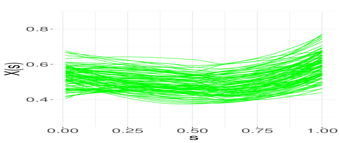
(a) CCA FA tract profile ($X$)

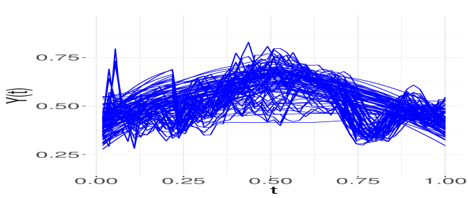
(b) RCST FA tract profile ($Y$)

Figure 1: The first 100 pairs of CCA and RCST FA tract profiles.

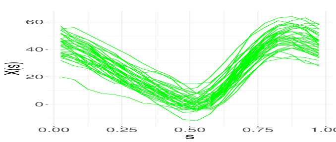
(a) Hip angle ($X$)

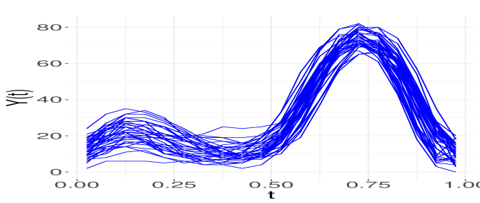
(b) Knee angle ($Y$)

Figure 2: Curves on boys’ hip and knee angles.

Analogous to simulation studies, the real data analysis ended up with slight difference among ReISPEs averages (resp. standard deviations), implying again the close accuracy of four competitors in prediction. fAPLS consumed much less time in analyzing DTI data, while this advantage did not exist for BG data. We guessed the small sample size ($n=39$) of BG data saved the computational burden of SigComp.

Table 1: The averages$\times 100$ (and standard deviations$\times 100$) of ReISPEs and ReISEEs in numerical experiments (running on a laptop with AMD^® Ryzen™ 5 4500U @$6\times 2.38$ GHz with 16 GB RAM). Values of $\rho$ and $\sigma_{\varepsilon}^{2}$ were designed, whereas SNR was computed accordingly. Row minimums are underlined.

	$\rho$	$\sigma_{\varepsilon}^{2}$	SNR	fAPLS	SigComp	NIPALS	SIMPLS
Estimation error: mean ReISEE$\times 100$ (standard deviation$\times 100$)
Simulation 1	0.1	1	10	33.04 (14.53)	72.63 (25.77)	73.02 (7.12)	42.18 (18.53)
		100	1	37.84 (8.80)	84.12 (21.39)	73.71 (5.96)	45.41 (14.27)
	0.9	1	11	33.20 (14.64)	72.60 (27.28)	71.82 (8.49)	42.21 (18.57)
		100	1	37.84 (10.22)	86.67 (23.26)	73.78 (6.53)	44.44 (16.77)
Simulation 2	0.1	1	7	0.89 (0.62)	1.35 (0.48)	7.44 (1.33)	0.95 (0.49)
		80	1	13.01 (3.23)	13.05 (5.50)	21.00 (6.69)	12.75 (3.79)
	0.9	1	7	1.42 (2.02)	1.68 (0.75)	7.90 (1.63)	1.64 (1.72)
		80	1	17.46 (15.45)	21.03 (16.43)	26.55 (12.73)	23.46 (20.67)
Simulation 3	0.1	0.05	7	2.33 (5.92)	8.98 (21.21)	4.28 (8.54)	1.99 (5.75)
		1	2	7.04 (4.25)	19.32 (26.67)	13.66 (20.08)	8.70 (15.92)
	0.9	0.05	7	6.27 (14.55)	6.62 (18.34)	6.22 (11.46)	5.33 (10.82)
		1	2	23.53 (30.15)	20.36 (27.07)	27.88 (32.14)	16.68 (26.25)
Prediction error: mean ReISPE$\times 100$ (standard deviation$\times 100$)
Simulation 1	0.1	1	10	1.65 (0.39)	1.74 (0.43)	1.94 (0.43)	1.80 (0.45)
		100	1	47.69 (5.37)	47.69 (5.40)	47.70 (5.37)	47.62 (5.37)
	0.9	1	11	1.56 (0.36)	1.62 (0.43)	1.85 (0.48)	1.71 (0.42)
		100	1	46.57 (6.10)	46.57 (6.09)	46.71 (6.08)	46.61 (6.07)
Simulation 2	0.1	1	7	2.69 (0.50)	2.57 (0.49)	2.69 (0.50)	2.69 (0.49)
		80	1	68.88 (5.33)	68.80 (5.64)	68.89 (5.33)	68.90 (5.40)
	0.9	1	7	2.68 (0.63)	2.56 (0.62)	2.70 (0.63)	2.70 (0.63)
		80	1	68.90 (6.35)	69.06 (6.48)	68.88 (6.39)	69.14 (6.43)
Simulation 3	0.1	0.05	7	28.68 (4.32)	28.62 (4.43)	28.61 (4.39)	28.56 (4.42)
		1	2	90.18 (3.48)	90.11 (3.38)	90.21 (3.59)	90.04 (3.50)
	0.9	0.05	7	28.37 (5.41)	28.11 (5.57)	28.33 (5.36)	28.37 (5.38)
		1	2	89.36 (4.40)	89.16 (4.92)	89.36 (4.48)	89.22 (4.70)
DTI	-	-	-	81.10 (3.51)	81.97 (3.94)	80.99 (3.69)	80.75 (3.59)
BG	-	-	-	62.65 (12.68)	71.23 (15.64)	69.41 (16.12)	65.04 (15.83)

Table 2: Averages (and standard deviations) of component numbers and total running time (in seconds) for numerical experiments (running on a laptop with AMD^® Ryzen™ 5 4500U @$6\times 2.38$ GHz with 16 GB RAM). Values of $\rho$ and $\sigma_{\varepsilon}^{2}$ were designed, whereas SNR was computed accordingly. Row minimums are underlined.

	$\rho$	$\sigma_{\varepsilon}^{2}$	SNR	fAPLS	SigComp	NIPALS	SIMPLS
Number of components: average number (standard deviation)
Simulation 1	0.1	1	10	2.2 (0.4)	2.2 (0.4)	2.1 (0.3)	2.2 (0.4)
		100	1	2.1 (0.3)	2.1 (0.4)	2.1 (0.3)	2.1 (0.4)
	0.9	1	11	2.2 (0.4)	2.2 (0.4)	2.2 (0.4)	2.2 (0.4)
		100	1	2.1 (0.3)	2.1 (0.4)	2.1 (0.3)	2.2 (0.4)
Simulation 2	0.1	1	7	6.2 (1.0)	3.1 (0.2)	10.3 (1.1)	9.9 (1.2)
		80	1	2.0 (0.3)	3.5 (1.1)	4.3 (1.3)	4.3 (1.3)
	0.9	1	7	6.5 (1.8)	3.0 (0.0)	10.2 (1.4)	10.0 (1.7)
		80	1	2.6 (1.9)	4.7 (1.3)	4.6 (1.8)	5.2 (2.7)
Simulation 3	0.1	0.05	7	1.9 (0.5)	1.4 (0.6)	2.2 (0.6)	1.8 (0.7)
		1	2	1.3 (0.5)	1.3 (0.5)	2.1 (0.4)	1.4 (0.6)
	0.9	0.05	7	2.1 (0.7)	1.5 (0.8)	2.3 (0.5)	2.0 (0.9)
		1	2	1.7 (0.9)	1.4 (0.7)	2.3 (0.6)	1.5 (0.8)
DTI	-	-	-	4.1 (0.8)	3.3 (0.7)	4.6 (0.5)	4.8 (0.4)
BG	-	-	-	2.7 (0.9)	4.1 (1.4)	5.0 (1.6)	4.9 (1.5)
Total running time in seconds for all replicates/splits
Simulation 1	0.1	1	10	3.0	41.8	350.3	150.2
		100	1	3.4	41.4	358.5	149.6
	0.9	1	11	3.4	41.2	327.2	148.7
		100	1	3.4	40.1	327.3	147.5
Simulation 2	0.1	1	7	36.1	48.6	398.5	241.7
		80	1	35.8	51.4	416.3	242.2
	0.9	1	7	35.7	50.1	375.0	242.3
		80	1	36.4	49.3	377.7	242.9
Simulation 3	0.1	0.05	7	6.9	41.6	327.9	163.2
		1	2	6.4	44.0	336.8	164.4
	0.9	0.05	7	6.4	41.0	272.0	162.8
		1	2	6.4	41.6	275.7	163.6
DTI	-	-	-	5.4	71.8	266.4	101.6
BG	-	-	-	1.6	1.7	29.2	23.5

4 Conclusion & discussion

Fitting FoFR, we suggest fAPLS, a route of FPLS via Krylov subspaces. The fAPLS estimator owns a concise and explicit expression. Meanwhile, we introduce an alternative but equivalent version, stabilizing numerical outputs. In spite of its less computational burden, fAPLS is fairly competitive to existing FPLS routes in terms of both estimation and prediction accuracy. Our proposal is potential to be further extended to more complex data structure, as illustrated in the following paragraphs.

More efforts can be put on the estimation of $r_{XX}$ and $r_{XY}$. To accommodate measurement errors, the local linear smoothing (see, e.g., Yao et al., 2005a; Li and Hsing, 2010) and spline smoothing (see, e.g., Xiao et al., 2018) may be helpful. In the case of geographic data, the spatial correlation (i.e., $X_{i}$ and $X_{i^{\prime}}$, $i\neq i^{\prime}$, no longer mutually independent) lead to a potential inconsistency of PLS estimators; see Singer et al. (2016, Theorem 1) for this issue in the multivariate context. A naive correction, transplanted from Singer et al. (2016, Section 4.1), is to instead implement the regression on transformed observations $(X_{i}^{*},Y_{i}^{*})$, $i=1,\ldots,n$, such that, for all $(s,t)\in\mathbb{I}_{X}\times\mathbb{I}_{Y}$, $[X_{1}^{*}(s),\ldots,X_{n}^{*}(s)]^{\top}=\bm{V}_{XX}^{-1/2}(s)[X_{1}(s),\ldots,X_{n}(s)]^{\top}$ and $[Y_{1}^{*}(t),\ldots,Y_{n}^{*}(t)]^{\top}=\bm{V}_{YY}^{-1/2}(t)[Y_{1}(t),\ldots,Y_{n}(t)]^{\top}$, with matrices $\bm{V}_{XX}(s)=[\operatorname*{cov}\{X_{i}(s),X_{i^{\prime}}(s)\}]_{n\times n}$ and $\bm{V}_{YY}(t)=[\operatorname*{cov}\{Y_{i}(t),Y_{i^{\prime}}(t)\}]_{n\times n}$. But it is even challenging to recover $\bm{V}_{XX}$ and $\bm{V}_{YY}$ sufficiently accurately without specifying the dependence structure, since there is only one observation for each $i$. Alternatively and more practically, one can target at correcting naive $\hat{r}_{XX}$ and $\hat{r}_{XY}$ for dependent subjects; Paul and Peng (2011) offered a solution to it.

fAPLS has got a heuristic extension to multiple functional covariates, i.e., associated with each realization $Y_{i}\sim Y$, there are $m>1$ functional covariates, say $X_{ij}\sim X_{\cdot j}$, $1\leq j\leq m$, and correspondingly $m$ coefficient functions $\beta^{*(j)}$, $1\leq j\leq m$. In particular,

$$Y_{i}(t)=\mu_{Y}(t)+\sum_{i=1}^{m}\mathcal{L}_{X_{ij}}(\beta^{*(j)})+\varepsilon_{i}(t),$$

where $Y_{i}$ and $X_{ij}$ are assumed to be independent across all $i$. Following the idea of (4), an ad hoc estimator for $(\beta^{*(1)},\ldots,\beta^{*(m)})$ is thus

$$(\hat{\beta}_{\rm fAPLS}^{(1)},\ldots,\hat{\beta}_{\rm fAPLS}^{(m)})=\operatorname*{arg\,min\,}_{\beta^{(j)}\in{\rm KS}_{p}(\widehat{\Gamma}_{X_{\cdot j}X_{\cdot j}},\beta^{*(j)}),\ 1\leq j\leq m}\frac{1}{m}\sum_{i=1}^{m}\int_{\mathbb{I}_{Y}}\Bigg{\{}Y_{i}(t)-\bar{Y}_{i}(t)\\ -\sum_{j=1}^{m}\int_{\mathbb{I}_{X_{\cdot j}}}(X_{ij}-\bar{X}_{\cdot j})(s)\beta^{(j)}(s,t){\rm d}s\Bigg{\}}^{2}{\rm d}t,$$

with $\bar{X}_{\cdot j}=m^{-1}\sum_{j=1}^{m}X_{ij}$ and domains $\mathbb{I}_{X_{\cdot j}}$ varying with $j$. Of course, it becomes necessary to introduce penalties once the above minimizer is not uniquely defined.

Although fAPLS appears to merely work for linear models, it is possible to be utilized in fitting the (functional) generalized linear models and proportional hazard models. The basic idea, inherited from Marx (1996), is to embed PLS routes into iteratively reweighted least squares (Green, 1984) in maximizing likelihood. Recent successful applications of this idea include Albaqshi (2017) and Wang et al. (2020). Once trajectories are sparsely and irregularly observed, fAPLS may be further modified in analogy to Zhou and Lockhart (2020).

Appendix A Appendix

In detail our assumptions are summarized as below.

1. $\sum_{j,j^{\prime}=1}^{\infty}\lambda_{j,X}^{-2}\left\{\int_{\mathbb{I}_{Y}}\int_{\mathbb{I}_{X}}\phi_{j,X}(s)r_{XY}(s,t)\phi_{j^{\prime},Y}(t){\rm d}s{\rm d}t\right\}^{2}<\infty$. $\beta^{*}$ belongs to ${\rm range}(\Gamma_{XX})=\{\Gamma_{XX}(f)\mid f\in L_{2}(\mathbb{I}_{X}\times\mathbb{I}_{Y})\}$.

2. $\operatorname*{E}(\|X\|_{2}^{4})<\infty$ for all $t\in\mathbb{I}_{Y}$.

3. As $n\to\infty$, $p=p(n)=O(n^{1/2})$.

4. Let $\mathbb{I}_{X}=[0,1]$. Both $\|\xi_{XX}\|_{\infty,2}$ and $\|\eta_{XX}\|_{\infty,2}$ are of order $O_{p}(1)$ as $n\to\infty$, with $\xi_{XX}$ and $\eta_{XX}$ defined as in Lemma A.1 and $\|\cdot\|_{\infty,2}$ defined such that $\|f\|_{\infty,2}=\sup_{s\in\mathbb{I}_{X}}\{\int_{\mathbb{I}_{X}}f^{2}(s,t){\rm d}t\}^{1/2}$ for $f\in L_{2}(\mathbb{I}_{X}\times\mathbb{I}_{X})$.

5. Additional requirements on $p$ vary with the magnitude of $\|r_{XX}\|_{2}$; they also depend on $\tau_{p}$, the smallest eigenvalue of $\bm{H}_{p}$.

   • If $\|r_{XX}\|_{2}\geq 1$, then, as $n\to\infty$, $n^{-1}\tau_{p}^{-2}p^{4}\|r_{XX}\|_{2}^{4p}\max(1,\tau_{p}^{-2}p^{2}\|r_{XX}\|_{2}^{4p})$ and $n^{-1}\tau_{p}^{-3}p^{5}\|r_{XX}\|_{2}^{6p}$ are both of order $o(1)$;

   • if $\|r_{XX}\|_{2}<1$, then $(n\tau_{p}^{4})^{-1}=o(1)$ as $n$ diverges.

6. Keep everything in (C5) but substitute $\|r_{XX}\|_{\infty}$ for $\|r_{XX}\|_{2}$. Meanwhile, require that $\|\beta_{p,\rm fAPLS}-\beta^{*}\|_{\infty}=o(1)$ as $p$ diverges, viz. an enhanced version of Proposition 1.

7. Stochastic process $Y$ is “eventually totally bounded in mean” (as defined by Hoffmann-Jørgensen, 1985, (5)–(7)); i.e., in our context,

   • $\operatorname*{E}(\|Y\|_{\infty})<\infty$;

   • for each $\epsilon>0$, there is a finite cover of $\mathbb{T}$, say ${\rm Cover}(\mathbb{T})$, for each set $\mathbb{A}\in{\rm Cover}(\mathbb{T})$, such that $\inf_{n\in\mathbb{Z}^{+}}n^{-1}\operatorname*{E}\{\sup_{t,t^{\prime}\in\mathbb{A}}|Y(t)-Y(t^{\prime})|\}<\epsilon$.

Introducing (C1), He et al. (2010, Theorem 2.3) confirmed the identifiability of $\beta^{*}$ for FoFR and derived (1). (C1) was also the foundation of Yao et al. (2005b). Assumptions (C2)–(C4) are prerequisites for the convergence of $\widehat{\Gamma}_{XX}^{j}(\beta^{*})$ ($=\widehat{\Gamma}_{XX}^{j-1}(\hat{r}_{XY})$) which is uniform in $j\geq 1$. One may feel unclear about the technical conditions stated in (C5) for the scenario of $\|r_{XX}\|_{2}\geq 1$: virtually a special case for is that $n^{-1}\max(\tau_{p}^{-4},\tau_{p}^{-6},\tau_{p}^{-8})=o(1)$ and $p=O(\ln\ln n)$. Apparently, $p$ is more restricted when $\|r_{XX}\|_{2}\geq 1$ than in the case of $\|r_{XX}\|_{2}<1$ (for the latter case $p$ is allowed to diverge at the rate of $O(n^{1/2})$); that is why Delaigle and Hall (2012) suggested changing the scale on which $X$ is measured. (C6) is stronger than (C5), enabling us to consider the $L_{\infty}$-convergence. At last, we add (C7) as a prerequisite for the uniform law of large numbers for $\{Y_{i}\mid i\geq 1\}$.

Lemma A.1.

For each $(s,s^{\prime},t)\in\mathbb{I}_{X}\times\mathbb{I}_{X}\times\mathbb{I}_{Y}$,

$$\hat{r}_{XX}(s,s^{\prime}) =r_{XX}(s,s^{\prime})+n^{-1/2}\xi_{XX}(s,s^{\prime})+n^{-1}\eta_{XX}(s,s^{\prime}),$$

$$\hat{r}_{XY}(s,t) =r_{XY}(s,t)+n^{-1/2}\xi_{XY}(s,t)+n^{-1}\eta_{XY}(s,t)$$ (16)

where, with identity operator $I:\mathbb{R}\to\mathbb{R}$,

$$\xi_{XX}(s,s^{\prime}) =\frac{1}{\sqrt{n}}\sum_{i=1}^{n}(I-\operatorname*{E})[\{X_{i}(s)-\mu_{X}(s)\}\{X_{i}(s^{\prime})-\mu_{X}(s^{\prime})\}],$$

$$\eta_{XX}(s,s^{\prime}) =-n\{\bar{X}(s)-\mu_{X}(s)\}\{\bar{X}(s^{\prime})-\mu_{X}(s^{\prime})\},$$

$$\xi_{XY}(s,t) =\frac{1}{\sqrt{n}}\sum_{i=1}^{n}(I-\operatorname*{E})[\{X_{i}(s)-\mu_{X}(s)\}\{Y_{i}(t)-\mu_{Y}(t)\}],$$

$$\eta_{XY}(s,t) =-n\{\bar{X}(s)-\mu_{X}(s)\}\{\bar{Y}(t)-\mu_{Y}(t)\},$$

and $\|\xi_{XX}\|_{2}$, $\|\eta_{XX}\|_{2}$, $\|\xi_{XY}\|_{2}$ and $\|\eta_{XY}\|_{2}$ all equal $O_{p}(1)$ as $n$ diverges.

Proof of Lemma A.1.

It is an immediate implication of Delaigle and Hall (2012, (5.1)). ∎

Lemma A.2.

Assume (C1) and (C2) and that there is $C>0$ such that, for all $n$, we have $p\leq Cn^{-1/2}$ (i.e., condition (C3)). Then, for each $\epsilon>0$, there are positive $C_{1}$, $C_{2}$ and $n_{0}$ such that, for each $n>n_{0}$,

$$\Pr\left[\bigcap_{j=1}^{p}\left\{\|\widehat{\Gamma}_{XX}^{j}(\beta^{*})-\Gamma_{XX}^{j}(\beta^{*})\|_{2}\leq n^{-1/2}\|r_{XX}\|_{2}^{j-1}\{C_{1}+C_{2}(j-1)\}\right\}\right]\geq 1-\epsilon.$$

Assuming one more condition (C4),

$$\Pr\left[\bigcap_{j=1}^{p}\left\{\|\widehat{\Gamma}_{XX}^{j}(\beta^{*})-\Gamma_{XX}^{j}(\beta^{*})\|_{\infty}\leq n^{-1/2}\|r_{XX}\|_{\infty}^{i-1}\{C_{1}+C_{2}(j-1)\}\right\}\right]\geq 1-\epsilon.$$

Proof of Lemma A.2.

Since $\Gamma_{XX}(\beta^{*})=r_{XY}$ and $\widehat{\Gamma}_{XX}(\beta^{*})=\hat{r}_{XY}$, Lemma A.2 is simply implied by Lemma A.1 when $p=1$. For integer $j\geq 2$ and each $(s,s^{\prime},t)\in\mathbb{I}_{X}\times\mathbb{I}_{X}\times\mathbb{I}_{Y}$,

$$|\widehat{\Gamma}_{XX}^{j}(\beta^{*})(s,t) -\Gamma_{XX}^{j}(\beta^{*})(s,t)|$$

$$= \ |\widehat{\Gamma}_{XX}\{\widehat{\Gamma}_{XX}^{j-1}(\beta^{*})-\Gamma_{XX}^{j-1}(\beta^{*})\}(s,t)+(\widehat{\Gamma}_{XX}-\Gamma_{XX})\{\Gamma_{XX}^{j-1}(\beta^{*})\}(s,t)|$$

$$\leq \ \left\{\int_{\mathbb{I}_{X}}\hat{r}_{XX}^{2}(s,s^{\prime}){\rm d}w\right\}^{1/2}\left[\int_{\mathbb{I}_{X}}\{\widehat{\Gamma}_{XX}^{j-1}(\beta^{*})-\Gamma_{XX}^{j-1}(\beta^{*})\}(s^{\prime},t){\rm d}w\right]^{1/2}$$

$$+\left[\int_{\mathbb{I}_{X}}\{\hat{r}_{XX}(s,s^{\prime})-r_{XX}(s,s^{\prime})\}^{2}{\rm d}s^{\prime}\right]^{1/2}\left\{\int_{\mathbb{I}_{X}}\Gamma_{XX}^{j-1}(\beta^{*})(s^{\prime},t){\rm d}s^{\prime}\right\}^{1/2}.$$

It implies that, by the triangle inequality,

$$\|\widehat{\Gamma}_{XX}^{j}(\beta^{*})-\Gamma_{XX}^{j}(\beta^{*})\|_{2}\leq\|\hat{r}_{XX}\|_{2}\|\widehat{\Gamma}_{XX}^{j-1}(\beta^{*})-\Gamma_{XX}^{j-1}(\beta^{*})\|_{2}+\|\hat{r}_{XX}-r_{XX}\|_{2}\|\Gamma_{XX}^{j-1}(\beta^{*})\|_{2}.$$

On iteration it gives that

$$\|\widehat{\Gamma}_{XX}^{j}(\beta^{*})-\Gamma_{XX}^{j}(\beta^{*})\|_{2}\leq\|\hat{r}_{XX}\|_{2}^{j-1}\|\widehat{\Gamma}_{XX}(\beta^{*})-\Gamma_{XX}(\beta^{*})\|_{2}\\ +\|\hat{r}_{XX}-r_{XX}\|_{2}\sum_{j^{\prime}=1}^{j-1}\|\hat{r}_{XX}\|_{2}^{j-j^{\prime}-1}\|\Gamma_{XX}^{j^{\prime}}(\beta^{*})\|_{2}.$$ (17)

For each $\epsilon>0$, there is $n_{0}>0$ such that, for all $n>n_{0}$, we have

$$1-\epsilon/2\leq \ \Pr(\|\hat{r}_{XX}-r_{XX}\|_{2}\leq C_{0}n^{-1/2})\leq\Pr(\|\hat{r}_{XX}\|_{2}\leq\|r_{XX}\|_{2}+C_{0}n^{-1/2}),$$

$$1-\epsilon/2\leq \ \Pr(\|\hat{r}_{XY}-r_{XY}\|_{2}\leq C_{0}n^{-1/2}),$$

with constant $C_{0}>0$, by Lemma A.1. It follows (17) that

$$1-\epsilon\leq\Pr\Bigg{[}\bigcap_{j=1}^{p}\Bigg{[}\|(\widehat{\Gamma}_{XX}^{j} -\Gamma_{XX}^{j})(\beta^{*})\|_{2}\leq C_{0}n^{-1/2}\Bigg{\{}(\|r_{XX}\|_{2}+C_{0}n^{-1/2})^{j-1}$$

$$+\sum_{j^{\prime}=1}^{j-1}\|r_{XX}\|_{2}^{j^{\prime}}\|\beta^{*}\|_{2}(\|r_{XX}\|_{2}+C_{0}n^{-1/2})^{j-j^{\prime}-1}\Bigg{\}}\Bigg{]}\Bigg{]}$$

$$\leq\Pr\Bigg{[}\bigcap_{j=1}^{p}\Bigg{[}\|(\widehat{\Gamma}_{XX}^{j} -\Gamma_{XX}^{j})(\beta^{*})\|_{2}\leq C_{0}n^{-1/2}\|r_{XX}\|_{2}^{j-1}\Bigg{\{}(1+C_{0}n^{-1/2}/\|r_{XX}\|_{2})^{j-1}$$

$$+\|\beta^{*}\|_{2}\sum_{j^{\prime}=1}^{j-1}(1+C_{0}n^{-1/2}/\|r_{XX}\|_{2})^{j-j^{\prime}-1}\Bigg{\}}\Bigg{]}\Bigg{]}$$

$$\leq\Pr\Bigg{[}\bigcap_{j=1}^{p}\Bigg{\{}\|\widehat{\Gamma}_{XX}^{j} (\beta^{*})-\Gamma_{XX}^{j}(\beta^{*})\|_{2}$$

$$\leq n^{-1/2}\|r_{XX}\|_{2}^{j-1}\{C_{1}+C_{2}(j-1)\}\Bigg{\}}\Bigg{]},\quad\text{(since $p\leq Cn^{1/2}$)}$$

where $C_{1}=C_{0}\exp(CC_{0}/\|r_{XX}\|_{2})$ and $C_{2}=\|\beta^{*}\|_{2}C_{1}$.

Suppose (C4) holds. Similar to (17),

$$\|\widehat{\Gamma}_{XX}^{j}(\beta^{*})-\Gamma_{XX}^{j}(\beta^{*})\|_{\infty}\leq \ \|\hat{r}_{XX}\|_{\infty}^{j-1}\|\widehat{\Gamma}_{XX}(\beta^{*})-\Gamma_{XX}(\beta^{*})\|_{\infty}$$

$$+\|\hat{r}_{XX}-r_{XX}\|_{\infty}\sum_{j^{\prime}=1}^{j-1}\|\hat{r}_{XX}\|_{\infty}^{j-j^{\prime}-1}\|\Gamma_{XX}^{j^{\prime}}(\beta^{*})\|_{\infty}$$

$$\leq \ \|\hat{r}_{XX}\|_{\infty}^{j-1}\|\widehat{\Gamma}_{XX}(\beta^{*})-\Gamma_{XX}(\beta^{*})\|_{\infty}$$

$$+\|\hat{r}_{XX}-r_{XX}\|_{\infty}\sum_{j^{\prime}=1}^{j-1}\|\hat{r}_{XX}\|_{\infty}^{j-j^{\prime}-1}\|r_{XX}\|_{\infty}^{j^{\prime}}\|\beta^{*}\|_{\infty}.$$

Mimicking the argument above for the $L_{2}$ sense, one obtains that

$$\Pr\left[\bigcap_{j=1}^{p}\left\{\|\widehat{\Gamma}_{XX}^{j}(\beta^{*})-\Gamma_{XX}^{j}(\beta^{*})\|_{\infty}\leq n^{-1/2}\|r_{XX}\|_{\infty}^{j-1}\{C_{1}+C_{2}(j-1)\}\right\}\right]\geq 1-\epsilon,$$

with, at this time, $C_{1}=C_{0}\exp(CC_{0}/\|r_{XX}\|_{\infty})$ and $C_{2}=\|\beta^{*}\|_{\infty}C_{1}$. The finiteness of $\|\beta^{*}\|_{\infty}$ originates from the continuity of eigenfunctions $\phi_{i,X}$’s and $\phi_{i,Y}$’s (refer to the Mercer’s theorem). ∎

Proof of Proposition 1.

Recall $\beta_{p,p^{\prime},\rm FPCR}$ at (2) and introduce $\beta_{p,\infty,\rm FPCR}\in L_{2}(\mathbb{I}_{X}\times\mathbb{I}_{Y})$ such that

$$\beta_{p,\infty,\rm FPCR}(s,t)=\lim_{p^{\prime}\to\infty}\beta_{p,p^{\prime},\rm FPCR}(s,t)=\sum_{j=1}^{p}\frac{\phi_{j,X}(s)}{\lambda_{j,X}}\int_{\mathbb{I}_{X}}\phi_{j,X}(s^{\prime})r_{XY}(s^{\prime},t){\rm d}s^{\prime}.$$

It follows that

$$\Gamma_{XX}(\beta_{p,\infty,\rm FPCR})(s,t)=\sum_{j=1}^{p}\phi_{j,X}(s)\int_{\mathbb{I}_{X}}\phi_{j,X}(s^{\prime})r_{XY}(s^{\prime},t){\rm d}w.$$

Now

$$[(\lambda_{1,X}I-\Gamma_{XX})\circ\cdots\circ(\lambda_{p,X}I-\Gamma_{XX})](\beta_{p,\infty,\rm FPCR})=0$$

in which the left-hand side equals $\sum_{i=j}^{p}a_{j}\Gamma_{XX}^{j}(\beta_{p,\infty,\rm FPCR})$ with $a_{0}=\prod_{j=1}^{p}\lambda_{j,X}>0$. Therefore,

$$\beta_{p,\infty,\rm FPCR}=-\sum_{j=1}^{p}\frac{a_{j}}{a_{0}}\Gamma_{XX}^{j}(\beta_{p,\infty,\rm FPCR}).$$

Denote by $P_{p}:{\rm range}(\Gamma_{XX})\to{\rm range}(\Gamma_{XX})$ the operator that projects elements in ${\rm range}(\Gamma_{XX})$ to ${\rm span}\{f_{jj^{\prime}}\in L_{2}(\mathbb{I}_{X}\times\mathbb{I}_{Y})\mid f_{jj^{\prime}}(s,t)=\phi_{j,X}(s)\phi_{j^{\prime},Y}(t),1\leq j\leq p,j^{\prime}\geq 1\}$. Thus $\beta_{p,\infty,\rm FPCR}=P_{p}(\beta^{*})$. Since $\Gamma_{XX}^{j}(\beta_{p,\infty,\rm FPCR})=P_{p}[\Gamma_{XX}^{j}(\beta^{*})]$, one has

$$P_{p}\left[\beta^{*}+\sum_{j=1}^{p}\frac{a_{j}}{a_{0}}\Gamma_{XX}^{j}(\beta^{*})\right]=0,$$

implying that, for all $p$,

$$P_{p}(\beta^{*})\in\{P_{p}(f)\mid f\in\overline{{\rm KS}_{\infty}(\Gamma_{XX},\beta^{*})}\}.$$

Taking limits as $p\rightarrow\infty$ on both sides of the above formula, we obtain $\beta^{*}\in\overline{{\rm KS}_{\infty}(\Gamma_{XX},\beta^{*})}$ and accomplish the proof. ∎

Proof of Proposition 2.

Recall $\beta_{p,\rm fAPLS}$ (4) and $\hat{\beta}_{p,\rm fAPLS}$ (9) and notations in defining them. The Cauchy-Schwarz inequality implies that

$$|\hat{h}_{jj^{\prime}} -h_{jj^{\prime}}|$$

$$\leq \ \|\widehat{\Gamma}_{XX}^{j}(\beta^{*})-\Gamma_{XX}^{j}(\beta^{*})\|_{2}\|\widehat{\Gamma}_{XX}^{j^{\prime}+1}(\beta^{*})\|_{2}+\|\widehat{\Gamma}_{XX}^{j^{\prime}+1}(\beta^{*})-\Gamma_{XX}^{j^{\prime}+1}(\beta^{*})\|_{2}\|\Gamma_{XX}^{j}(\beta^{*})\|_{2}$$

$$\leq \ \|\widehat{\Gamma}_{XX}^{j}(\beta^{*})-\Gamma_{XX}^{j}(\beta^{*})\|_{2}\|\hat{r}_{XX}\|_{2}^{j+1}\|\beta^{*}\|_{2}+\|\widehat{\Gamma}_{XX}^{j^{\prime}+1}(\beta^{*})-\Gamma_{XX}^{j^{\prime}+1}(\beta^{*})\|_{2}\|r_{XX}\|_{2}^{j}\|\beta^{*}\|_{2}.$$

By Lemmas A.1 and A.2, for each $\epsilon>0$ and $p\leq Cn^{1/2}$, there are positive $n_{0}$, $C_{3}$ and $C_{4}$ such that, for all $n>n_{0}$,

$$1-\epsilon\leq\Pr\Bigg{[}\bigcap_{j,j^{\prime}=1}^{p}\Big{\{}|\hat{h}_{jj^{\prime}}-h_{jj^{\prime}}|\leq \|\widehat{\Gamma}_{XX}^{j}(\beta^{*})-\Gamma_{XX}^{j}(\beta^{*})\|_{2}(\|r_{XX}\|_{2}+C_{0}n^{-1/2})^{j^{\prime}+1}\|\beta^{*}\|_{2}$$

$$+\|\widehat{\Gamma}_{XX}^{j^{\prime}+1}(\beta^{*})-\Gamma_{XX}^{j^{\prime}+1}(\beta^{*})\|_{2}\|r_{XX}\|_{2}^{j}\|\beta^{*}\|_{2}\Big{\}}\Bigg{]}$$

$$\leq\Pr\Bigg{[}\bigcap_{j,j^{\prime}=1}^{p}\Big{\{}|\hat{h}_{jj^{\prime}}-h_{jj^{\prime}}|\leq \ n^{-1/2}\|r_{XX}\|_{2}^{i+j^{\prime}}\{C_{3}\max(j,j^{\prime})+C_{4}\}\Big{\}}\Bigg{]}.$$

Thus

$$\|\widehat{\bm{H}}_{p}-\bm{H}_{p}\|_{2}^{2}\leq \sum_{j,j^{\prime}=1}^{p}|\hat{h}_{jj^{\prime}}-h_{jj^{\prime}}|^{2}$$

$$= \ O_{p}\left(n^{-1}\sum_{j,j^{\prime}=1}^{p}\|r_{XX}\|_{2}^{2j+2j^{\prime}}\right)+O_{p}\left\{n^{-1}\sum_{j,j^{\prime}=1}^{p}\max(j^{2},j^{\prime 2})\|r_{XX}\|_{2}^{2j+2j^{\prime}}\right\}$$

$$= \ \begin{cases}O_{p}(n^{-1}p^{2}\|r_{XX}\|_{2}^{4p})+O_{p}(n^{-1}p^{4}\|r_{XX}\|_{2}^{4p})&\text{if }\|r_{XX}\|_{2}\geq 1\\ O_{p}(n^{-1})&\text{if }\|r_{XX}\|_{2}<1\end{cases}$$

$$= \ \begin{cases}O_{p}(n^{-1}p^{4}\|r_{XX}\|_{2}^{4p})&\text{if }\|r_{XX}\|_{2}\geq 1\\ O_{p}(n^{-1})&\text{if }\|r_{XX}\|_{2}<1.\end{cases}$$ (18)

Here $\|\cdot\|_{2}$ is abused for the matrix norm induced by the Euclidean norm, i.e., for arbitrary $\bm{A}\in\mathbb{R}^{p\times p^{\prime}}$ and $\bm{b}\in\mathbb{R}^{p^{\prime}\times 1}$ $\|\bm{A}\|_{2}=\sup_{\bm{b}:\|\bm{b}\|_{2}=1}\|\bm{A}\bm{b}\|_{2}$ is actually the largest eigenvalue of $\bm{A}$. It reduces to the Euclidean norm for vectors. It is analogous to (18) to deduce that

$$\|\widehat{\bm{\alpha}}_{p}-\bm{\alpha}_{p}\|_{2}^{2}=\sum_{j=1}^{p}|\hat{\alpha}_{j}-\alpha_{j}|^{2}=\ \begin{cases}O_{p}(n^{-1}p^{3}\|r_{XX}\|_{2}^{2p})&\text{if }\|r_{XX}\|_{2}\geq 1\\ O_{p}(n^{-1})&\text{if }\|r_{XX}\|_{2}<1.\end{cases}$$ (19)

Denote by $\tau_{p}$ the smallest eigenvalue of $\bm{H}_{p}$. Noting that $\|\bm{H}_{p}^{-1}\|_{2}=\tau_{p}^{-1}$, for $p\leq Cn^{1/2}$,

$$\|(\widehat{\bm{H}}_{p}-\bm{H}_{p})\bm{H}_{p}^{-1}\|_{2}\leq\tau_{p}^{-1}\|\widehat{\bm{H}}_{p}-\bm{H}_{p}\|_{2}=\begin{cases}O_{p}(n^{-1/2}\tau_{p}^{-1}p^{2}\|r_{XX}\|_{2}^{2p})&\text{if }\|r_{XX}\|_{2}\geq 1\\ O_{p}(n^{-1/2}\tau_{p}^{-1})&\text{if }\|r_{XX}\|_{2}<1.\end{cases}$$

Introduce random matrix $\bm{M}_{p}\in\mathbb{R}^{p\times p}$ such that $\bm{I}-\bm{H}_{p}^{-1}(\widehat{\bm{H}}_{p}-\bm{H}_{p})+\bm{M}_{p}=\{\bm{I}+\bm{H}_{p}^{-1}(\widehat{\bm{H}}_{p}-\bm{H}_{p})\}^{-1}$, i.e., $\bm{M}_{p}=\{\bm{I}+\bm{H}_{p}^{-1}(\widehat{\bm{H}}_{p}-\bm{H}_{p})\}^{-1}\bm{H}_{p}^{-1}(\widehat{\bm{H}}_{p}-\bm{H}_{p})\bm{H}_{p}^{-1}(\widehat{\bm{H}}_{p}-\bm{H}_{p}).$ Therefore,

$$\|\bm{M}_{p}\|_{2}\leq\|\bm{I}+\bm{H}^{-1}(\widehat{\bm{H}}_{p}-\bm{H}_{p})\|_{2}^{-1}\|\bm{H}^{-1}(\widehat{\bm{H}}_{p}-\bm{H}_{p})\|_{2}^{2}\leq(1-\rho)^{-1}\tau_{p}^{-2}\|\widehat{\bm{H}}_{p}-\bm{H}_{p}\|_{2}^{2},$$

provided that $\tau_{p}^{-1}\|\widehat{\bm{H}}_{p}-\bm{H}_{p}\|_{2}\leq\rho<1$ (refer to Delaigle and Hall, 2012, (7.18)). Revealed by the identity that $\widehat{\bm{H}}_{p}^{-1}=\{\bm{I}+\bm{H}_{p}^{-1}(\widehat{\bm{H}}_{p}-\bm{H}_{p})\}^{-1}\bm{H}_{p}^{-1}$,

$$\|\widehat{\bm{H}}_{p}^{-1} -\bm{H}_{p}^{-1}\|_{2}$$

$$\leq \ \{\|\bm{H}_{p}^{-1}(\widehat{\bm{H}}_{p}-\bm{H}_{p})\|_{2}+\|\bm{M}_{p}\|_{2}\}\|\bm{H}_{p}^{-1}\|_{2}$$

$$= \ \begin{cases}O_{p}(n^{-1/2}\tau_{p}^{-2}p^{2}\|r_{XX}\|_{2}^{2p})+O_{p}(n^{-1}\tau_{p}^{-3}p^{4}\|r_{XX}\|_{2}^{4p})&\text{if }\|r_{XX}\|_{2}\geq 1\\ O_{p}(n^{-1/2}\tau_{p}^{-2})+O_{p}(n^{-1}\tau_{p}^{-3})&\text{if }\|r_{XX}\|_{2}<1.\end{cases}$$ (20)

Combining (19), (20) and the identity that

$$\|\bm{\alpha}_{p}\|_{2}= \ \left[\sum_{j=1}^{p}\left\{\int_{\mathbb{I}_{Y}}\int_{\mathbb{I}_{X}}r_{XY}(s,t)\Gamma_{XX}^{j}(\beta^{*})(s,s^{\prime}){\rm d}s{\rm d}s^{\prime}\right\}^{2}\right]^{1/2}$$

$$\leq \ \left[\sum_{j=1}^{p}\|r_{XY}\|_{2}^{2}\|\Gamma_{XX}^{j}(\beta^{*})\|_{2}^{2}\right]^{1/2}$$

$$= \ \begin{cases}O(p^{1/2}\|r_{XX}\|_{2}^{p})&\text{if }\|r_{XX}\|_{2}\geq 1\\ O(1)&\text{if }\|r_{XX}\|_{2}<1,\end{cases}$$ (21)

we reach that

$$\|\widehat{\bm{H}}_{p}^{-1} \widehat{\bm{\alpha}}_{p}-\bm{H}_{p}^{-1}\bm{\alpha}_{p}\|_{2}$$

$$\leq \ \|\widehat{\bm{H}}_{p}^{-1}\|_{2}\|\widehat{\bm{\alpha}}_{p}-\bm{\alpha}_{p}\|_{2}+\|\widehat{\bm{H}}_{p}^{-1}-\bm{H}_{p}^{-1}\|_{2}\|\bm{\alpha}_{p}\|_{2}$$

$$= \ \begin{cases}O_{p}(n^{-1/2}\tau_{p}^{-1}p^{3/2}\|r_{XX}\|_{2}^{p})\\ \qquad+\ O_{p}(n^{-1/2}\tau_{p}^{-2}p^{5/2}\|r_{XX}\|_{2}^{3p})+O_{p}(n^{-1}\tau_{p}^{-3}p^{9/2}\|r_{XX}\|_{2}^{5p})&\text{if }\|r_{XX}\|_{2}\geq 1\\ O_{p}(n^{-1/2}\tau_{p}^{-1})+O_{p}(n^{-1/2}\tau_{p}^{-2})+O_{p}(n^{-1}\tau_{p}^{-3})&\text{if }\|r_{XX}\|_{2}<1\end{cases}$$

$$= \ \begin{cases}O_{p}(n^{-1/2}\tau_{p}^{-1}p^{3/2}\|r_{XX}\|_{2}^{p})\\ \qquad+\ O_{p}(n^{-1/2}\tau_{p}^{-2}p^{5/2}\|r_{XX}\|_{2}^{3p})+O_{p}(n^{-1}\tau_{p}^{-3}p^{9/2}\|r_{XX}\|_{2}^{5p})&\text{if }\|r_{XX}\|_{2}\geq 1\\ O_{p}(n^{-1/2}\tau_{p}^{-2})+O_{p}(n^{-1}\tau_{p}^{-3})\quad\text{(since $\tau_{p}\leq h_{jj}=O(1)$)}&\text{if }\|r_{XX}\|_{2}<1.\end{cases}$$ (22)

For each $(s,t)\in\mathbb{I}_{X}\times\mathbb{I}_{Y}$,

$$|\hat{\beta}_{p,\rm fAPLS}(s,t) -\beta_{p,\rm fAPLS}(s,t)|^{2}$$

$$= \ \Bigg{|}[\widehat{\Gamma}_{XX}(\beta^{*})(s,s^{\prime}),\ldots,\widehat{\Gamma}_{XX}^{p}(\beta^{*})(s,s^{\prime})]\widehat{\bm{H}}_{p}^{-1}\widehat{\bm{\alpha}}_{p}$$

$$-[\Gamma_{XX}(\beta^{*})(s,s^{\prime}),\ldots,\Gamma_{XX}^{p}(\beta^{*})(s,s^{\prime})]\bm{H}_{p}^{-1}\bm{\alpha}_{p}\Bigg{|}^{2}$$

$$\leq \ \Bigg{|}\|\widehat{\bm{H}}_{p}^{-1}\widehat{\bm{\alpha}}_{p}-\bm{H}_{p}^{-1}\bm{\alpha}_{p}\|_{2}\left[\sum_{j=1}^{p}\{\widehat{\Gamma}_{XX}^{j}(\beta^{*})(s,s^{\prime})\}^{2}\right]^{1/2}$$

$$+\|\bm{H}_{p}^{-1}\bm{\alpha}_{p}\|_{2}\left[\sum_{j=1}^{p}[\{\widehat{\Gamma}_{XX}^{j}-\Gamma_{XX}^{j}\}(\beta^{*})(s,s^{\prime})]^{2}\right]^{1/2}\Bigg{|}^{2}$$

$$\leq \ 2\|\widehat{\bm{H}}_{p}^{-1}\widehat{\bm{\alpha}}_{p}-\bm{H}_{p}^{-1}\bm{\alpha}_{p}\|_{2}^{2}\left[\sum_{j=1}^{p}\{\widehat{\Gamma}_{XX}^{j}(\beta^{*})(s,s^{\prime})\}^{2}\right]$$

$$+2\|\bm{H}_{p}^{-1}\bm{\alpha}_{p}\|_{2}^{2}\left[\sum_{j=1}^{p}\{\widehat{\Gamma}_{XX}^{j}(\beta^{*})(s,s^{\prime})-\Gamma_{XX}^{j}(\beta^{*})(s,s^{\prime})\}^{2}\right].$$

Thus $\|\hat{\beta}_{p,\rm fAPLS}-\beta_{p,\rm fAPLS}\|_{2}$ is bounded as below:

$$\| \hat{\beta}_{p,\rm fAPLS}-\beta_{p,\rm fAPLS}\|_{2}^{2}$$

$$\leq \ 2\|\widehat{\bm{H}}_{p}^{-1}\widehat{\bm{\alpha}}_{p}-\bm{H}_{p}^{-1}\bm{\alpha}_{p}\|_{2}^{2}\sum_{j=1}^{p}\|\Gamma_{XX}^{j}(\beta^{*})\|_{2}^{2}+2\|\bm{H}_{p}^{-1}\bm{\alpha}_{p}\|_{2}^{2}\sum_{j=1}^{p}\|\Gamma_{XX}^{j}(\beta^{*})-\widehat{\Gamma}_{XX}^{j}(\beta^{*})\|_{2}^{2}$$

$$\leq \ 2\|\widehat{\bm{H}}_{p}^{-1}\widehat{\bm{\alpha}}_{p}-\bm{H}_{p}^{-1}\bm{\alpha}_{p}\|_{2}^{2}\sum_{j=1}^{p}\|\Gamma_{XX}^{j}(\beta^{*})\|_{2}^{2}$$ (23)

$$+2\tau_{p}^{-2}\|\bm{\alpha}_{p}\|_{2}^{2}\sum_{j=1}^{p}\|\widehat{\Gamma}_{XX}^{j}(\beta^{*})-\Gamma_{XX}^{j}(\beta^{*})\|_{2}^{2},$$ (24)

where, owing to (22),

$$\eqref{eq:beta.dist.1}=\begin{cases}O_{p}(n^{-1}\tau_{p}^{-2}p^{4}\|r_{XX}\|_{2}^{4p})\\ \qquad+\ O_{p}(n^{-1}\tau_{p}^{-4}p^{6}\|r_{XX}\|_{2}^{8p})+O_{p}(n^{-2}\tau_{p}^{-6}p^{10}\|r_{XX}\|_{2}^{12p})&\text{if }\|r_{XX}\|_{2}\geq 1\\ O_{p}(n^{-1}\tau_{p}^{-4})+O_{p}(n^{-2}\tau_{p}^{-6})&\text{if }\|r_{XX}\|_{2}<1;\end{cases}$$

the order of (24) is jointly given by (21) and Lemma A.2, i.e.,

$$\eqref{eq:beta.dist.2}=\begin{cases}O(n^{-1}\tau_{p}^{-2}p^{4}\|r_{XX}\|_{2}^{4p})&\text{if }\|r_{XX}\|_{2}\geq 1\\ O_{p}(n^{-1}\tau_{p}^{-2})&\text{if }\|r_{XX}\|_{2}<1.\end{cases}$$

In this way we deduce

$$\| \hat{\beta}_{p,\rm fAPLS}-\beta_{p,\rm fAPLS}\|_{2}^{2}$$

$$= \ \begin{cases}O_{p}(n^{-1}\tau_{p}^{-2}p^{4}\|r_{XX}\|_{2}^{4p})\\ \qquad+\ O_{p}(n^{-1}\tau_{p}^{-4}p^{6}\|r_{XX}\|_{2}^{8p})+O_{p}(n^{-2}\tau_{p}^{-6}p^{10}\|r_{XX}\|_{2}^{12p})&\text{if }\|r_{XX}\|_{2}\geq 1\\ O_{p}(n^{-1}\tau_{p}^{-4})+O_{p}(n^{-2}\tau_{p}^{-6})&\text{if }\|r_{XX}\|_{2}<1.\end{cases}$$ (25)

A set of necessary conditions for the zero-convergence (in probability) of (25) is contained in (C5). Once they are fulfilled, we conclude the $L_{2}$ convergence (in probability) of $\hat{\beta}_{p,\rm fAPLS}$ to $\beta^{*}$ following Proposition 1.

We complete the proof by bounding the estimating error in the supremum metric:

$$\| \hat{\beta}_{p,\rm fAPLS}-\beta_{p,\rm fAPLS}\|_{\infty}^{2}$$

$$= \ \left\|[\widehat{\Gamma}_{XX}(\beta^{*}),\ldots,\widehat{\Gamma}_{XX}^{p}(\beta^{*})]\widehat{\bm{H}}_{p}^{-1}\widehat{\bm{\alpha}}_{p}-[\Gamma_{XX}(\beta^{*}),\ldots,\Gamma_{XX}^{p}(\beta^{*})]\bm{H}_{p}^{-1}\bm{\alpha}_{p}\right\|_{\infty}^{2}$$

$$\leq \ 2\|\widehat{\bm{H}}_{p}^{-1}\widehat{\bm{\alpha}}_{p}-\bm{H}_{p}^{-1}\bm{\alpha}_{p}\|_{2}^{2}\sum_{j=1}^{p}\|\Gamma_{XX}^{j}(\beta^{*})\|_{\infty}^{2}+2\|\bm{H}_{p}^{-1}\bm{\alpha}_{p}\|_{2}^{2}\sum_{i=1}^{p}\|\Gamma_{XX}^{j}(\beta^{*})-\widehat{\Gamma}_{XX}^{j}(\beta^{*})\|_{\infty}^{2}$$

$$\leq \ 2\|\widehat{\bm{H}}_{p}^{-1}\widehat{\bm{\alpha}}_{p}-\bm{H}_{p}^{-1}\bm{\alpha}_{p}\|_{2}^{2}\sum_{j=1}^{p}\|\Gamma_{XX}^{j}(\beta^{*})\|_{\infty}^{2}\quad\text{(compare \eqref{eq:beta.dist.1})}$$

$$+2\tau_{p}^{-2}\|\bm{\alpha}_{p}\|_{2}^{2}\sum_{j=1}^{p}\|\widehat{\Gamma}_{XX}^{i}(\beta^{*})-\Gamma_{XX}^{j}(\beta^{*})\|_{\infty}^{2},\quad\text{(compare \eqref{eq:beta.dist.2})}$$

$$= \ \begin{cases}O_{p}(n^{-1}\tau_{p}^{-2}p^{4}\|r_{XX}\|_{\infty}^{4p})\\ \qquad+\ O_{p}(n^{-1}\tau_{p}^{-4}p^{6}\|r_{XX}\|_{\infty}^{8p})+O_{p}(n^{-2}\tau_{p}^{-6}p^{10}\|r_{XX}\|_{\infty}^{12p})&\text{if }\|r_{XX}\|_{\infty}\geq 1\\ O_{p}(n^{-1}\tau_{p}^{-4})+O_{p}(n^{-2}\tau_{p}^{-6})&\text{if }\|r_{XX}\|_{\infty}<1,\end{cases}$$

converging to zero (in probability) with the satisfaction of (C6). The zero-convergence (in probability) of $\|\hat{\beta}_{p,\rm fAPLS}-\beta^{*}\|_{\infty}$ follows if we assume that $\|\beta_{p,\rm fAPLS}-\beta^{*}\|_{\infty}\to 0$ as $p$ diverges. ∎

Proof of Proposition 3.

Notice that

$$\|\hat{g}_{p,\rm fAPLS}(X_{0}) -g(X_{0})\|_{2}$$

$$\leq \ \|\bar{Y}-\mu_{Y}\|_{2}+\|\bar{X}-\mu_{X}\|_{2}\|\beta^{*}\|_{2}+\|X_{0}-\bar{X}\|_{2}\|\hat{\beta}_{p,\rm fAPLS}-\beta^{*}\|_{2},$$

$$\|\hat{g}_{p,\rm fAPLS}(X_{0}) -g(X_{0})\|_{\infty}$$

$$\leq \ \|\bar{Y}-\mu_{Y}\|_{\infty}+\|\bar{X}-\mu_{X}\|_{2}\|\beta^{*}\|_{\infty}+\|X_{0}-\bar{X}\|_{2}\|\hat{\beta}_{p,\rm fAPLS}-\beta^{*}\|_{\infty}.$$

The finite trace of $R_{XX}$ (resp. $R_{YY}$), viz. $\sum_{j=1}^{\infty}\lambda_{j,X}=\operatorname*{E}(\|X-\mu_{X}\|_{2}^{2})<\infty$ (resp. $\sum_{j=1}^{\infty}\lambda_{j,Y}=\operatorname*{E}(\|Y-\mu_{Y}\|_{2}^{2})<\infty$), entails that $\|\bar{X}-\mu_{X}\|_{2}=o_{\rm a.s.}(1)$ (resp. $\|\bar{Y}-\mu_{Y}\|_{2}=o_{\rm a.s.}(1)$); see Hoffmann-Jørgensen and Pisier (1976, (2.1.3)). The proof is complete once we verify the zero-convergence (in probability and under (C7)) of $\|\bar{Y}-\mu_{Y}\|_{\infty}$ following Hoffmann-Jørgensen (1985, Theorem 2). ∎

References

• Albaqshi (2017) Albaqshi, A. M. H. (2017). Generalized Partial Least Squares Approach for Nominal Multinomial Logit Regression Models with a Functional Covariate. Ph. D. thesis, University of Northern Colorado.
• Alexander et al. (2007) Alexander, A. L., J. E. Lee, M. Lazar, and A. S. Field (2007). Diffusion tensor imaging of the brain. Neurotherapeutics 4, 316–329.
• Benatia et al. (2017) Benatia, D., M. Carrasco, and J.-P. Florens (2017). Functional linear regression with functional response. J. Econom. 201, 269–291.
• Beyaztas and Shang (2020) Beyaztas, U. and H. L. Shang (2020). On function-on-function regression: partial least squares approach. Environ. Ecol. Stat. 27, 95–114.
• Bissett (2015) Bissett, A. C. (2015). Improvements to PLS Methodology. Ph. D. thesis, University of Manchester.
• Cook and Forzani (2019) Cook, R. D. and L. Forzani (2019). Partial least squares prediction in high-dimensional regression. Ann. Stat. 47, 884–908.
• de Jong (1993) de Jong, S. (1993). SIMPLS: An alternative approach to partial least squares regression. Chemometrics Intell. Lab. Syst. 18, 251–263.
• Delaigle and Hall (2012) Delaigle, A. and P. Hall (2012). Methodology and theory for partial least squares applied to functional data. Ann. Stat. 40, 322–352.
• Goldsmith et al. (2011) Goldsmith, J., J. Bob, C. M. Crainiceanu, B. Caffo, and D. Reich (2011). Penalized functional regression. J. Comput. Graph. Stat. 20, 830–851.
• Goldsmith et al. (2019) Goldsmith, J., F. Scheipl, L. Huang, J. Wrobel, J. Gellar, J. Harezlak, M. W. McLean, B. Swihart, L. Xiao, C. Crainiceanu, and P. T. Reiss (2019). refund: Regression with Functional Data. R package version 0.1-21.
• Green (1984) Green, P. J. (1984). Iteratively reweighted least squares for maximum likelihood estimation, and some robust and resistant alternatives. J. R. Stat. Soc. Ser. B-Stat. Methodol. 46, 149–192.
• He et al. (2010) He, G., H.-G. Müller, J.-L. Wang, and W. Yang (2010). Functional linear regression via canonical analysis. Bernoulli 16, 705–729.
• Hochstrasser (1972) Hochstrasser, U. W. (1972). Orthogonal polynomials. In M. Abramowitz and I. A. Stegun (Eds.), Handbook of Mathematical Functions with Formulas, Graphs, and Mathematical Tables, Applied Mathematics Series 55, pp.  773–802. New York: Dover Publications, Inc. Tenth original printing with corrections.
• Hoffmann-Jørgensen (1985) Hoffmann-Jørgensen, J. (1985). Necessary and sufficient condition for the uniform law of large numbers. In A. Beck, R. Dudley, M. Hahn, J. Kuelbs, and M. Marcus (Eds.), Probability in Banach Spaces V, Volume 1153 of Lecture Notes in Mathematics, pp.  258–272. Berlin: Springer.
• Hoffmann-Jørgensen and Pisier (1976) Hoffmann-Jørgensen, J. and G. Pisier (1976). The law of large numbers and the central limit theorem in Banach spaces. Ann. Probab. 4, 587–599.
• Ivanescu et al. (2015) Ivanescu, A. E., A.-M. Staicu, F. Scheipl, and S. Greven (2015). Penalized function-on-function regression. Comput. Stat. 30, 539–568.
• Lange (2010) Lange, K. (2010). Numerical Analysis for Statisticians (2nd ed.). New York: Springer.
• Li and Hsing (2010) Li, Y. and T. Hsing (2010). Uniform convergence rates for nonparametric regression and principal component analysis in functional/longitudinal data. Ann. Stat. 38, 3321–3351.
• Lian (2015) Lian, H. (2015). Minimax prediction for functional linear regression with functional responses in reproducing kernel hilbert spaces. J. Multivariate Anal. 140, 395–402.
• Luo and Qi (2017) Luo, R. and X. Qi (2017). Function-on-function linear regression by signal compression. J. Am. Stat. Assoc. 112, 690–705.
• Luo and Qi (2018) Luo, R. and X. Qi (2018). FRegSigCom: Functional Regression using Signal Compression Approach. R package version 0.3.0.
• Marx (1996) Marx, B. D. (1996). Iteratively reweighted partial least squares estimation for generalized linear regression. Technometrics 38, 374–381.
• Paul and Peng (2011) Paul, D. and J. Peng (2011). Principal components analysis for sparsely observed correlated functional data using a kernel smoothing approach. Electron. J. Statist. 5, 1960–2003.
• Ramsay and Dalzell (1991) Ramsay, J. O. and C. J. Dalzell (1991). Some tools for functional data analysis. J. R. Stat. Soc. Ser. B-Stat. Methodol. 53, 539–572.
• Ramsay et al. (2020) Ramsay, J. O., H. Wickham, S. Graves, and G. Hooker (2020). fda: Functional Data Analysis. R package version 5.1.4.
• Singer et al. (2016) Singer, M., T. Krivobokova, A. Munk, and B. de Groot (2016). Partial least squares for dependent data. Biometrika 103, 351–362.
• Sun et al. (2018) Sun, X., P. Du, X. Wang, and P. Ma (2018). Optimal penalized function-on-function regression under a reproducing kernel hilbert space framework. J. Am. Stat. Assoc. 113, 1601–1611.
• Tasaki (2009) Tasaki, H. (2009). Convergence rates of approximate sums of riemann integrals. J. Approx. Theory 161, 477–490.
• Wang et al. (2020) Wang, Y., J. G. Ibrahim, and H. Zhu (2020). Partial least squares for functional joint models with applications to the alzheimer’s disease neuroimaging initiative study. Biometrics. in press.
• Wold (1975) Wold, H. (1975). Path models with latent variables: the NIPALS approach. In H. Blalock, A. Aganbegian, F. M. Borodkin, R. Boudon, and V. Capecchi (Eds.), Quantitative Sociology: International Perspectives on Mathematical and Statistical Model Building, pp.  307–335. New York: Academic Press.
• Xiao (2019) Xiao, L. (2019). Asymptotic theory of penalized splines. Electron. J. Statist. 13, 747–794.
• Xiao et al. (2018) Xiao, L., C. Li, W. Checkley, and C. Crainiceanu (2018). Fast covariance estimation for sparse functional data. Stat. Comput. 28, 511–522.
• Yao et al. (2005a) Yao, F., H.-G. Müller, and J.-L. Wang (2005a). Functional data analysis for sparse longitudinal data. J. Am. Stat. Assoc. 100, 577–590.
• Yao et al. (2005b) Yao, F., H.-G. Müller, and J.-L. Wang (2005b). Functional linear regression analysis for longitudinal data. Ann. Stat. 33, 2873–2903.
• Zhou and Lockhart (2020) Zhou, Z. and R. Lockhart (2020). Partial least squares for sparsely observed curves with measurement errors. arXiv:2003.11542.