$F_{K}/F_{\pi}$ from Möbius domain-wall fermions solved on gradient-flowed HISQ ensembles

Abstract

We report the results of a lattice quantum chromodynamics calculation of $F_{K}/F_{\pi}$ using Möbius domain-wall fermions computed on gradient-flowed $N_{f}=2+1+1$ highly-improved staggered quark ensembles. The calculation is performed with five values of the pion mass ranging from $130\lesssim m_{\pi}\lesssim 400$ MeV, four lattice spacings of $a\sim 0.15,0.12,0.09$ and $0.06$ fm and multiple values of the lattice volume. The interpolation/extrapolation to the physical pion and kaon mass point, the continuum, and infinite volume limits are performed with a variety of different extrapolation functions utilizing both the relevant mixed-action effective field theory expressions as well as discretization-enhanced continuum chiral perturbation theory formulas. We find that the $a\sim 0.06$ fm ensemble is helpful, but not necessary to achieve a subpercent determination of $F_{K}/F_{\pi}$. We also include an estimate of the strong isospin breaking corrections and arrive at a final result of $F_{\hat{K}^{+}}/F_{\hat{\pi}^{+}}=1.1942(45)$ with all sources of statistical and systematic uncertainty included. This is consistent with the Flavour Lattice Averaging Group average value, providing an important benchmark for our lattice action. Combining our result with experimental measurements of the pion and kaon leptonic decays leads to a determination of $|V_{us}|/|V_{ud}|=0.2311(10)$.

I Introduction

Leptonic decays of the charged pions and kaons provide a means for probing flavor-changing interactions of the Standard Model (SM). In particular, the SM predicts that the Cabibbo-Kobayashi-Maskawa (CKM) matrix is unitary, providing strict constraints on various sums of the matrix elements. Thus, a violation of these constraints is indicative of new, beyond the SM physics. There is a substantial flavor physics program dedicated to searching indirectly for potential violations.

CKM matrix elements may be determined through a combination of experimental leptonic decay widths and theoretical determinations of the meson decay constants. For example, the ratio of the kaon and pion decay constants, $F_{K},F_{\pi}$, respectively, may be related to the ratio of light and strange CKM matrix elements $|V_{us}|,|V_{ud}|$ via Marciano (2004); Aubin et al. (2004),

$$\frac{\Gamma(K\to l\bar{\nu}_{l})}{\Gamma(\pi\to l\bar{\nu}_{l})} =\frac{|V_{us}|^{2}}{|V_{ud}|^{2}}\frac{F_{K}^{2}}{F_{\pi}^{2}}\frac{m_{K}}{m_{\pi}}\frac{\left(1-\frac{m_{l}^{2}}{m_{K}^{2}}\right)^{2}}{\left(1-\frac{m_{l}^{2}}{m_{\pi}^{2}}\right)^{2}}$$

$$\phantom{=}\times\left[1+{\delta}_{\mathrm{EM}}+{\delta}_{SU(2)}\right]\,.$$ (1)

In this expression, $l=e,\mu$, the one-loop radiative quantum electrodynamics (QED) correction is $\delta_{\mathrm{EM}}$ Decker and Finkemeier (1995); Finkemeier (1996) and ${\delta}_{SU(2)}$ is the strong isospin breaking correction that relates $F_{K}^{2}/F_{\pi}^{2}$ in the isospin limit to $F_{K^{+}}^{2}/F_{\pi^{+}}^{2}$ that includes $m_{d}-m_{u}$ corrections Cirigliano and Neufeld (2011)

$$\frac{F_{\hat{K}^{+}}^{2}}{F_{\hat{\pi}^{+}}^{2}}=\frac{F_{K}^{2}}{F_{\pi}^{2}}\left[1+{\delta}_{SU(2)}\right]\,.$$

Using lattice quantum chromodynamics (QCD) calculations of the ratio of decay constants in the above expression yields one of the most precise determinations of $|V_{us}|/|V_{ud}|$ Tanabashi et al. (2018). Combining the results obtained through lattice QCD with independent determinations of the CKM matrix elements, such as semileptonic meson decays, provides a means for testing the unitarity of the CKM matrix and obtaining signals of new physics.

$F_{K}/F_{\pi}$ is a so-called gold-plated quantity Davies et al. (2004) for calculating within lattice QCD. This dimensionless ratio skirts the issue of determining a physical scale for the lattices, and gives precise results due to the correlated statistical fluctuations between numerator and denominator, as well as the lack of signal-to-noise issues associated with calculations involving, for instance, nucleons. Lattice QCD calculations of $F_{K}/F_{\pi}$ are now a mature endeavor, with state-of-the-art calculations determining this quantity consistently with subpercent precision. The most recent review by the Flavour Lattice Averaging Group (FLAG), which performs global averages of quantities that have been calculated and extrapolated to the physical point by multiple groups, quotes a value of

$$\frac{F_{\hat{K}^{+}}}{F_{\pi^{+}}}=1.1932(19)$$ (2)

for $N_{f}=2+1+1$ dynamical quark flavors, including strong-isospin breaking corrections Aoki et al. (2019).

This average includes calculations derived from two different lattice actions, one Carrasco et al. (2015) with twisted-mass fermions Frezzotti and Rossi (2004a, b) and the other two Dowdall et al. (2013); Bazavov et al. (2018) with the highly improved staggered quark (HISQ) action Follana et al. (2007). The results obtained using the HISQ action are approximately seven times more precise than those from twisted mass and so the universality of the continuum limit for $F_{K}/F_{\pi}$ from $N_{f}=2+1+1$ results has not been tested with precision yet: in the continuum limit, all lattice actions should reduce to a single universal limit, that of SM QCD, provided all systematics are properly accounted for. Thus, in addition to lending more confidence to its global average, the calculation of a gold-plated quantity also allows for precise testing of new lattice actions, and the demonstration of control over systematic uncertainties for a given action. FLAG also reports averages for $N_{F}=2+1$, $F_{K^{\pm}}/F_{\pi^{\pm}}=1.1917(37)$ from Refs. Follana et al. (2008); Bazavov et al. (2010a); Durr et al. (2010); Blum et al. (2016); Dürr et al. (2017); Bornyakov et al. (2017) and for $N_{f}=2$, $F_{K^{\pm}}/F_{\pi^{\pm}}=1.1205(18)$ from Refs. Blossier et al. (2009), though we restrict our direct comparisons to the $N_{f}=2+1+1$ results just for simplicity.

In this work, we report a new determination of $F_{K}/F_{\pi}$ calculated with Möbius domain-wall fermions computed on gradient-flowed $N_{f}=2+1+1$ HISQ ensembles Berkowitz et al. (2017a). Our final result in the isospin symmetric limit, Sec. IV.4, including a breakdown in terms of statistical ($s$), pion and kaon mass extrapolation ($\chi$), continuum limit ($a$), infinite volume limit ($V$), physical point (phys) and model selection ($M$) uncertainties, is

$$\frac{F_{K}}{F_{\pi}} =1.1964(32)^{s}(12)^{\chi}(20)^{a}(01)^{V}(15)^{\rm phys}(12)^{M}$$

$$=1.1964(44)\,.$$ (3)

With our estimated strong isospin breaking corrections, Sec. IV.5, our result including $m_{d}-m_{u}$ effects is

$$\frac{F_{\hat{K}^{+}}}{F_{\hat{\pi}^{+}}} =1.1942(44)(07)^{\rm iso}$$

$$=1.1942(45)\,,$$ (4)

where the first uncertainty in the first line is the combination of those in Eq. (I).

In the following sections we will discuss details of our lattice calculation, including a brief synopsis of the action and ensembles used, as well as our strategy for extracting the relevant quantities from correlation functions. We will then detail our procedure for extrapolating to the physical point via combined continuum, infinite volume, and physical pion and kaon mass limits and the resulting uncertainty breakdown. We discuss the impact of the $a\sim 0.06$ fm ensemble on our analysis, the convergence of the $SU(3)$-flavor chiral expansion, and the estimate of the strong isospin breaking corrections. We conclude with an estimate of the impact our result has on improving the extraction of $|V_{us}|/|V_{ud}|$ and an outlook.

II Details of the lattice calculation

II.1 MDWF on gradient-flowed HISQ

Table 1: Input parameters for our lattice action. The abbreviated ensemble name Bhattacharya et al. (2015) indicates the approximate lattice spacing in fm and pion mass in MeV. The S, L, XL which come after an ensemble name denote a relatively small, large and extra-large volume with respect to $m_{\pi}L=4$.

Ensemble	$\beta$	$N_{\rm cfg}$	volume	$am_{l}$	$am_{s}$	$am_{c}$	$L_{5}/a$	$aM_{5}$	$b_{5},c_{5}$	$am_{l}^{\rm val}$	$am^{\rm res}_{l}\times 10^{4}$	$am_{s}^{\rm val}$	$am^{\rm res}_{s}\times 10^{4}$	${\sigma}$	$N$	$N_{\rm src}$
a15m400	5.80	1000	$16^{3}\times 48$	0.0217	0.065	0.838	12	1.3	1.50, 0.50	0.0278	9.365(87)	0.0902	6.937(63)	3.0	30	8
a15m350	5.80	1000	$16^{3}\times 48$	0.0166	0.065	0.838	12	1.3	1.50, 0.50	0.0206	9.416(90)	0.0902	6.688(62)	3.0	30	16
a15m310	5.80	1000	$16^{3}\times 48$	0.013	0.065	0.838	12	1.3	1.50, 0.50	0.0158	9.563(67)	0.0902	6.640(44)	4.2	45	24
a15m220	5.80	1000	$24^{3}\times 48$	0.0064	0.064	0.828	16	1.3	1.75, 0.75	0.00712	5.736(38)	0.0902	3.890(25)	4.5	60	16
a15m135XL	5.80	1000	$48^{3}\times 64$	0.002426	0.06730	0.8447	24	1.3	2.25, 1.25	0.00237	2.706(08)	0.0945	1.860(09)	3.0	30	32
a12m400	6.00	1000	$24^{3}\times 64$	0.0170	0.0509	0.635	8	1.2	1.25, 0.25	0.0219	7.337(50)	0.0693	5.129(35)	3.0	30	8
a12m350	6.00	1000	$24^{3}\times 64$	0.0130	0.0509	0.635	8	1.2	1.25, 0.25	0.0166	7.579(52)	0.0693	5.062(34)	3.0	30	8
a12m310	6.00	1053	$24^{3}\times 64$	0.0102	0.0509	0.635	8	1.2	1.25, 0.25	0.0126	7.702(52)	0.0693	4.950(35)	3.0	30	8
a12m220S	6.00	1000	$24^{4}\times 64$	0.00507	0.0507	0.628	12	1.2	1.50, 0.50	0.00600	3.990(42)	0.0693	2.390(24)	6.0	90	4
a12m220	6.00	1000	$32^{3}\times 64$	0.00507	0.0507	0.628	12	1.2	1.50, 0.50	0.00600	4.050(20)	0.0693	2.364(15)	6.0	90	4
a12m220L	6.00	1000	$40^{3}\times 64$	0.00507	0.0507	0.628	12	1.2	1.50, 0.50	0.00600	4.040(26)	0.0693	2.361(19)	6.0	90	4
a12m130	6.00	1000	$48^{3}\times 64$	0.00184	0.0507	0.628	20	1.2	2.00, 1.00	0.00195	1.642(09)	0.0693	0.945(08)	3.0	30	32
a09m400	6.30	1201	$32^{3}\times 64$	0.0124	0.037	0.44	6	1.1	1.25, 0.25	0.0160	2.532(23)	0.0491	1.957(17)	3.5	45	8
a09m350	6.30	1201	$32^{3}\times 64$	0.00945	0.037	0.44	6	1.1	1.25, 0.25	0.0121	2.560(24)	0.0491	1.899(16)	3.5	45	8
a09m310	6.30	780	$32^{3}\times 96$	0.0074	0.037	0.44	6	1.1	1.25, 0.25	0.00951	2.694(26)	0.0491	1.912(15)	6.7	167	8
a09m220	6.30	1001	$48^{3}\times 96$	0.00363	0.0363	0.43	8	1.1	1.25, 0.25	0.00449	1.659(13)	0.0491	0.834(07)	8.0	150	6
a09m135	6.30	1010	$64^{3}\times 96$	0.001326	0.03636	0.4313	12	1.1	1.50, 0.50	0.00152	0.938(06)	0.04735	0.418(04)	3.5	45	16
a06m310L	6.72	1000	$72^{3}\times 96$	0.0048	0.024	0.286	6	1.0	1.25, 0.25	0.00617	0.225(03)	0.0309	0.165(02)	3.5	45	8

There are many choices for discretizing QCD, with each choice being commonly referred to as a lattice action. These actions correspond to different UV theories that share a common low-energy theory, QCD. Sufficiently close to the continuum limit, the discrete lattice actions can be expanded as a series of local operators known as the Symanzik expansion Symanzik (1983a, b), the low-energy effective field theory (EFT) for the discrete lattice action. The Symanzik EFT contains a series of operators having higher dimension than those in QCD, multiplied by appropriate powers of the lattice spacing, $a$. For all lattice actions, the only operators of mass-dimension $\leq 4$ are those of QCD, such that the explicit effects from the various discretizations are encoded only in higher-dimensional operators which are all irrelevant in the renormalization sense. There is a universality of the continuum limit, $a\rightarrow 0$, in that all lattice actions, if calculated using sufficiently small lattice spacing, will recover the target theory of QCD, provided there are no surprises from nonperturbative effects.

Performing lattice QCD calculations with different actions is therefore valuable to test this universality, to help ensure a given action is not accidentally in a different phase of QCD, and to protect against unknown systematic uncertainties arising from a particular calculation with a particular action. In this work, we use a mixed-action Renner et al. (2005) in which the discretization scheme for the valence quarks is the Möbius domain-wall fermion (MDWF) action Brower et al. (2005, 2006, 2012) while the discretization scheme for the sea-quarks is the HISQ action Follana et al. (2007). Before solving the MDWF propagators, we apply a gradient-flow Narayanan and Neuberger (2006); Lüscher and Weisz (2011); Lüscher (2013) smoothing algorithm Lüscher (2010); Lohmayer and Neuberger (2011) to the gluons to dampen UV fluctuations, which also significantly improves the chiral symmetry properties of the MDWF action Berkowitz et al. (2017a) (for example, the residual chiral symmetry breaking scale of domain-wall fermions $m^{\rm res}$ is held to less than 10% of $m_{l}$ for reasonable values of $L_{5}$ and $M_{5}$, see Tab. 1). Our motivation to perform this calculation is to improve our understanding of $F_{K}/F_{\pi}$ and to test the MDWF on gradient-flowed HISQ action we have used to compute the $\pi^{-}\rightarrow\pi^{+}$ neutrinoless double beta decay matrix elements arising from prospective higher-dimension lepton-number-violating physics Nicholson et al. (2018), and the axial coupling of the nucleon $g_{A}$ Berkowitz et al. (2017b); Chang et al. (2018). As there is an otherwise straightforward path to determining $g_{A}$ to subpercent precision with pre-exascale computing such as Summit at Oak Ridge Leadership Computing Facility (OLCF) and Lassen at Lawrence Livermore National Laboratory (LLNL) Berkowitz et al. (2018a), it is important to ensure this action is consistent with known results at this level of precision.

There are several motivations for choosing this mixed-action (MA) scheme Renner et al. (2005); Bar et al. (2003). The MILC Collaboration provides their gauge configurations to any interested party and we have made heavy use of them. They have generated the configurations covering a large parameter space allowing one to fully control the physical pion mass, infinite volume and continuum limit extrapolations Bazavov et al. (2010b, 2013). The good chiral symmetry properties of the Domain Wall (DW) action Kaplan (1992); Shamir (1993); Furman and Shamir (1995) significantly suppress sources of chiral symmetry breaking from any sea-quark action, motivating the use of this mixed-action setup. While this action is not unitary at finite lattice spacing, we have tuned the valence quark masses such that the valence pion mass matches the taste-5 HISQ pion mass within a few percent, so as the continuum limit is taken, we recover a unitary theory.

EFT can be used to understand the salient features of such mixed-action lattice QCD (MALQCD) calculations. Chiral perturbation theory ($\chi$PT) Langacker and Pagels (1973); Gasser and Leutwyler (1984); Leutwyler (1994) can be extended to incorporate discretization effects into the analytic formula describing the quark-mass dependence of various hadronic quantities Sharpe and Singleton (1998). The MA EFT Bar et al. (2004) for DW valence fermions on dynamical rooted staggered fermions is well developed Bar et al. (2005); Tiburzi (2005); Chen et al. (2006, 2007); Orginos and Walker-Loud (2008); Jiang (2007); Chen et al. (2009a, b). The use of valence fermions which respect chiral symmetry leads to a universal form of the MA EFT extrapolation formulas at next-to-leading order (NLO) in the joint quark mass and lattice spacing expansions Chen et al. (2007, 2009a), which follows from the suppression of chiral symmetry breaking discretization effects.

II.2 Correlation function construction and analysis

The correlation function construction and analysis follows closely the strategy of Ref. Berkowitz et al. (2017a) and Berkowitz et al. (2017b); Chang et al. (2018). Here we summarize the relevant details for this work.

The pseudoscalar decay constants $F$ can be obtained from standard two-point correlation functions by making use of the 5D Ward-Takahashi identity Blum et al. (2004); Aoki et al. (2004)

$$F^{q_{1}q_{2}}=z_{0p}^{q_{1}q_{2}}\frac{m^{q_{1}}+m_{\textrm{res}}^{q_{1}}+m^{q_{2}}+m_{\textrm{res}}^{q_{2}}}{\left(E_{0}^{q_{1}q_{2}}\right)^{3/2}},$$ (5)

where $q_{1}$ and $q_{2}$ denote the quark content of the meson with lattice input masses $m_{q_{1}}$ and $m_{q_{2}}$ respectively. The point-sink ground-state overlap-factor $z_{0p}$ and ground-state energy $E_{0}$ are extracted from a two-point correlation function analysis with the model

$$C^{q_{1}q_{2}}_{(ss)ps}(t)=\sum_{n}z_{n(s)p}^{q_{1}q_{2}}z_{ns}^{q_{1}q_{2}\dagger}\left(e^{-E_{n}^{q_{1}q_{2}}t}+e^{-E_{n}^{q_{1}q_{2}}(T-t)}\right),$$ (6)

where $n$ encompasses in general an infinite tower of states, $t$ is the source-sink time separation, $T$ is the temporal box size and we have both smeared ($s$) and point ($p$) correlation functions which both come from smeared sources. From Ref. Berkowitz et al. (2017a), we show that gradient-flow smearing leads to the suppression of the domain-wall fermion oscillating mode (which also decouples as $M_{5}\rightarrow 1$, at least in free-field Syritsyn and Negele (2007)), and therefore this mode is not included in the correlator fit model. Finally, the residual chiral symmetry breaking $m_{\textrm{res}}$ is calculated by the ratio of two-point correlation functions evaluated at the midpoint of the fifth dimension $L_{5}/2$ and bounded on the domain wall Brower et al. (2012)

$$m_{\textrm{res}}(t)=\frac{\sum_{\mathbf{x}}\langle\pi(t,\mathbf{x},L_{5}/2)\pi(0,\mathbf{0},0)\rangle}{\sum_{\mathbf{x}}\langle\pi(t,\mathbf{x},0)\pi(0,\mathbf{0},0)\rangle},$$ (7)

where $\pi(t,\mathbf{x},s)\equiv\bar{q}(t,\mathbf{x},w)\gamma_{5}q(t,\mathbf{x},w)$ is the pseudoscalar interpolating operator at time $t$, space $\mathbf{x}$ and fifth dimension $s$. We extract $m_{\textrm{res}}$ by fitting Eq. (7) to a constant.

II.2.1 Analysis strategy

For all two-point correlation function parameters (MDWF and mixed MDWF-HISQ), we infer posterior parameter distributions in a Bayesian framework using a 4-state model which simultaneously describes the smeared- and point-sink two-point correlation functions (the source is always smeared). The joint posterior distribution is approximated by a multivariate normal distribution (we later refer to this procedure as fitting). The two-point correlation functions are folded in time to double the statistics. The analysis of the pion, kaon, $\bar{s}\gamma_{5}s$, and mixed MDWF-HISQ mesons are performed independently, with correlations accounted for under bootstrap resampling.

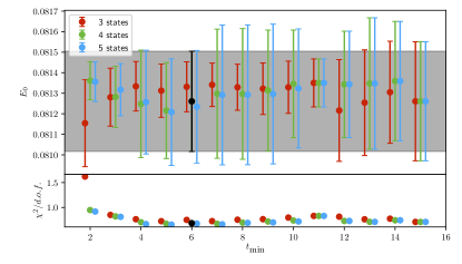
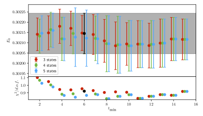
Figure 1: Stability of the ground-state mass determination of the pion (top) and kaon (bottom) on the a12m130 ensemble. The x-axis is the value of $t_{\rm min}$ used in the analysis and the resulting $E_{0}$ for a given $t_{\rm min}$ and number of states in the analysis is plotted. The 68% confidence interval of the chosen fit (black) is plotted as a horizontal band to guide the eye.

We analyze data of source-sink time separations between 0.72 and 3.6 fm for all 0.09 fm and 0.12 fm lattice spacing two-point correlation functions, and separations between 0.75 and 3.6 fm for all 0.15 fm lattice spacing two-point correlation functions.

We choose normally distributed priors for the ground-state energy and all overlap factors, and log-normal distributions for excited-state energy priors. The ground-state energy and overlap factors are motivated by the plateau values of the effective masses and scaled correlation function, and a prior width of 10% of the central value. The excited-state energy splittings are set to the value of two pion masses with a width allowing for fluctuations down to one pion mass within one standard deviation. The excited-state overlap factors are set to zero, with a width set to the mean value of the ground-state overlap factor.

Additionally, we fit a constant to the correlation functions in Eq. (7). For the 0.09 and 0.12 fm ensembles, we analyze source-sink separations that are greater than 0.72 fm. For the 0.12 fm ensemble, the minimum source-sink separation is 0.75 fm. The prior distribution for the residual chiral symmetry breaking parameter is set to the observed value per ensemble, with a width that is 100% of the central value. The uncertainty is propagated with bootstrap resampling.

We emphasize that all input fit parameters (i.e. number of states, fit region, priors) are chosen to have the same values in physical units for all observables, to the extent that a discretized lattice allows. Additionally, we note that the extracted ground-state observables from these correlation functions are insensitive to variations around the chosen set of input fit parameters. Fig. 1 shows the stability of the determination of $E_{0}$ for the pion and kaon on the a12m130 ensemble versus $t_{\rm min}$ and the number of states.

Table 2: Extracted masses and decay constants from correlation functions. An HDF5 file is provided with this publication which includes the resulting bootstrap samples which can be used to construct the correlated uncertainties. The small parameters in this table are defined as ${\epsilon}_{\pi,K}=m_{\pi,K}/(4\pi F_{\pi})$, ${\epsilon}_{a}=a/(2w_{0})$. The normalization of ${\epsilon}_{a}$ is chosen such that as a small parameter, it spans the range of ${\epsilon}_{\pi}^{2}\lesssim{\epsilon}_{a}^{2}\lesssim{\epsilon}_{K}^{2}$.

Ensemble	$am_{\pi}$	$am_{K}$	${\epsilon}_{\pi}^{2}$	${\epsilon}_{K}^{2}$	$m_{\pi}L$	${\epsilon}_{a}^{2}$	${\alpha}_{S}$	$aF_{\pi}$	$aF_{K}$	$F_{K}/F_{\pi}$
a15m400	0.30281(31)	0.42723(27)	0.09216(33)	0.18344(62)	4.85	0.19378(13)	0.58801	0.07938(12)	0.08504(09)	1.0713(09)
a15m350	0.26473(30)	0.41369(28)	0.07505(28)	0.18326(60)	4.24	0.19378(13)	0.58801	0.07690(11)	0.08370(09)	1.0884(09)
a15m310	0.23601(29)	0.40457(25)	0.06223(17)	0.18285(48)	3.78	0.19378(13)	0.58801	0.07529(09)	0.08293(09)	1.1015(13)
a15m220	0.16533(19)	0.38690(21)	0.03269(11)	0.17901(48)	3.97	0.19378(13)	0.58801	0.07277(08)	0.08196(10)	1.1263(15)
a15m135XL	0.10293(07)	0.38755(14)	0.01319(05)	0.18704(59)	4.94	0.19378(13)	0.58801	0.07131(11)	0.08276(10)	1.1606(18)
a12m400	0.24347(16)	0.34341(14)	0.08889(30)	0.17685(63)	5.84	0.12376(18)	0.53796	0.06498(11)	0.06979(07)	1.0739(17)
a12m350	0.21397(20)	0.33306(16)	0.07307(37)	0.17704(83)	5.14	0.12376(18)	0.53796	0.06299(14)	0.06851(07)	1.0876(27)
a12m310	0.18870(17)	0.32414(21)	0.05984(25)	0.17657(69)	4.53	0.12376(18)	0.53796	0.06138(11)	0.06773(10)	1.1033(21)
a12m220S	0.13557(32)	0.31043(22)	0.03384(19)	0.1774(10)0	3.25	0.12376(18)	0.53796	0.05865(16)	0.06673(11)	1.1378(27)
a12m220L	0.13402(15)	0.31021(19)	0.03289(15)	0.17621(79)	5.36	0.12376(18)	0.53796	0.05881(13)	0.06631(17)	1.1276(29)
a12m220	0.13428(17)	0.31001(17)	0.03314(15)	0.17666(81)	4.30	0.12376(18)	0.53796	0.05870(13)	0.06636(11)	1.1306(22)
a12m130	0.08126(16)	0.30215(11)	0.01287(08)	0.17788(71)	3.90	0.12376(18)	0.53796	0.05701(11)	0.06624(08)	1.1619(21)
a09m400	0.18116(15)	0.25523(13)	0.08883(32)	0.17633(59)	5.80	0.06515(08)	0.43356	0.04837(08)	0.05229(07)	1.0810(09)
a09m350	0.15785(20)	0.24696(12)	0.07256(32)	0.17761(68)	5.05	0.06515(08)	0.43356	0.04663(08)	0.05127(07)	1.0994(10)
a09m310	0.14072(12)	0.24106(14)	0.06051(22)	0.17757(59)	4.50	0.06515(08)	0.43356	0.04552(07)	0.05053(08)	1.1101(16)
a09m220	0.09790(06)	0.22870(09)	0.03307(14)	0.18045(70)	4.70	0.06515(08)	0.43356	0.04284(08)	0.04899(07)	1.1434(18)
a09m135	0.05946(06)	0.21850(08)	0.01346(08)	0.18175(91)	3.81	0.06515(08)	0.43356	0.04079(10)	0.04804(06)	1.1778(22)
a06m310L	0.09456(06)	0.16205(07)	0.06141(35)	0.1803(10)0	6.81	0.02726(03)	0.29985	0.03037(08)	0.03403(07)	1.1205(17)

III Extrapolation Functions

We now turn to the extrapolation/interpolation to the physical point. We have three ensembles at the physical pion mass with relatively high statistics and precise determinations of $F_{K}/F_{\pi}$ (a15m135XL, a12m130, and a09m135, see Tab. 2) such that the physical quark mass extrapolation is an interpolation. Nevertheless, we explore how the ensembles with heavier pion masses impact the physical point prediction and we use our dataset to explore uncertainty arising in the $SU(3)$-flavor chiral expansion.

We begin by assuming a canonical power-counting scheme for our MALQCD action Bar et al. (2005) in which $\mathrm{O}(m_{\pi}^{2})\sim\mathrm{O}(m_{K}^{2})\sim\mathrm{O}(a^{2}{\Lambda}_{\rm QCD}^{4})$ are all treated as small scales. For the quark mass expansion, the dimensionless small parameters $(m_{P}/4\pi F)^{2}$ naturally emerge from $\chi$PT where $P\in\{\pi,K,\eta\}$. For the discretization corrections, while $a{\Lambda}_{\rm QCD}^{2}$ is often used to estimate the relative size of corrections compared to typical hadronic mass scales, it is a bit unnatural to use this in a low-energy EFT as ${\Lambda}_{\rm QCD}$ is a QCD scale that does not emerge in $\chi$PT.

We chose to use another hadronic scale to form a dimensionless parameter with $a$, that being the gradient flow scale $w_{0}\sim 0.17$ fm Borsanyi et al. (2012). This quantity is easy to compute, has mild quark mass dependence, and the value is roughly $w_{0}^{-1}\simeq 4\pi F_{\pi}$. We then define the dimensionless small parameters for controlling the expansion to be

$${\epsilon}_{P}^{2}=\left(\frac{m_{P}}{{\Lambda}_{\chi}}\right)^{2}=\left(\frac{m_{P}}{4\pi F}\right)^{2}, {\epsilon}_{a}^{2}=\left(\frac{a}{2w_{0}}\right)^{2}.$$ (8)

We leave $F$ ambiguous, as we will explore taking $F=F_{\pi}$, $F=F_{K}$ and $F^{2}=F_{\pi}F_{K}$ in our definition of ${\Lambda}_{\chi}$. This particular choice of ${\epsilon}_{a}$ is chosen such that the range of values of this small parameter roughly corresponds to ${\epsilon}_{\pi}^{2}\lesssim{\epsilon}_{a}^{2}\lesssim{\epsilon}_{K}^{2}$ as the lattice spacing is varied, similar to the variation of ${\epsilon}_{\pi}^{2}$ itself over the range of pion masses used, see Tab. 2. As we will discuss in Sec. IV, this choice of ${\epsilon}_{a}$ seems natural as determined by the size of the discretization low-energy constants (LECs) which are found in the analysis. Note, this differs from the choice used in our analysis of $g_{A}$ Berkowitz et al. (2017b); Chang et al. (2018).

With this power-counting scheme, the different orders in the expansion are defined to be

$$\begin{array}[]{rl}\text{NLO:}&\mathrm{O}({\epsilon}_{P}^{2})\sim\mathrm{O}({\epsilon}_{a}^{2}),\\ \text{N${}^{2}$LO:}&\mathrm{O}({\epsilon}_{P}^{4})\sim\mathrm{O}({\epsilon}_{P}^{2}{\epsilon}_{a}^{2})\sim\mathrm{O}({\epsilon}_{a}^{4}),\\ \text{N${}^{3}$LO:}&\mathrm{O}({\epsilon}_{P}^{6})\sim\mathrm{O}({\epsilon}_{P}^{4}{\epsilon}_{a}^{2})\sim\mathrm{O}({\epsilon}_{P}^{2}{\epsilon}_{a}^{4})\sim\mathrm{O}({\epsilon}_{a}^{6}).\end{array}$$ (9)

Even at finite lattice spacing, $F_{K}=F_{\pi}$ in the $SU(3)$ flavor symmetry limit, also known as the $SU(3)$ vector limit $SU(3)_{V}$, and so there cannot be a pure $\mathrm{O}({\epsilon}_{a}^{2})$ correction as it must accompany terms which vanish in the $SU(3)_{V}$ limit, such as ${\epsilon}_{K}^{2}-{\epsilon}_{\pi}^{2}$. Therefore, at NLO, there cannot be any counterterms proportional to ${\epsilon}_{a}^{2}$ and the only discretization effects that can appear at NLO come through modification of the various meson masses that appear in the MA EFT.

We find that the precision of our results requires including terms higher than NLO, and we have to work at a hybrid N³LO order to obtain a good description of our data. Therefore, we will begin with a discussion of the full N²LO $\chi$PT theory expression for $F_{K}/F_{\pi}$ in the continuum limit Amoros et al. (2000); Ananthanarayan et al. (2017, 2018a, 2018b).

III.1 N²LO $\chi$PT

The analytic expression for $F_{K}/F_{\pi}$ up to N²LO is Ananthanarayan et al. (2018b)

$$\frac{F_{K}}{F_{\pi}} =1+\frac{5}{8}\ell_{\pi}-\frac{1}{4}\ell_{k}-\frac{3}{8}\ell_{\eta}+4{\bar{L}}_{5}({\epsilon}_{K}^{2}-{\epsilon}_{\pi}^{2})$$

$$\phantom{=}+{\epsilon}_{K}^{4}F_{F}\left(\frac{m_{\pi}^{2}}{m_{K}^{2}}\right)+\hat{K}_{1}^{r}{\lambda}_{\pi}^{2}+\hat{K}_{2}^{r}{\lambda}_{\pi}{\lambda}_{K}$$

$$\phantom{=}+\hat{K}_{3}^{r}{\lambda}_{\pi}{\lambda}_{\eta}+\hat{K}_{4}^{r}{\lambda}_{K}^{2}+\hat{K}_{5}^{r}{\lambda}_{K}{\lambda}_{\eta}+\hat{K}_{6}^{r}{\lambda}_{\eta}^{2}$$

$$\phantom{=}+\hat{C}_{1}^{r}{\lambda}_{\pi}+\hat{C}_{2}^{r}{\lambda}_{K}+\hat{C}_{3}^{r}{\lambda}_{\eta}+\hat{C}_{4}^{r}\,.$$ (10)

The first line is the LO (1) plus NLO terms, while the next three lines are the N²LO terms. Several nonunique choices were made to arrive at this formula. Prior to discussing these choices, we first define the parameters appearing in Eq. (III.1). First, the small parameters were all defined as

$${\epsilon}_{P}^{2}=\left(\frac{m_{P}}{4\pi F_{\pi}(m_{P})}\right)^{2}\,,$$ (11)

where $F_{\pi}(m_{P})$ is the “on-shell” pion decay constant at the masses $m_{P}$. The quantities $\ell_{P}$ are defined as

$$\ell_{P}={\epsilon}_{P}^{2}\ln\left(\frac{m_{P}^{2}}{\mu^{2}}\right)\,,$$ (12)

where $\mu$ is a renormalization scale. The coefficient $\bar{L}_{5}=(4\pi)^{2}L_{5}^{r}(\mu)$ is one of the regulated Gasser-Leutwyler LECs Gasser and Leutwyler (1985) which has a renormalization scale dependence that exactly cancels against the dependence arising from the logarithms appearing at the same order. In the following, we define all of the Gasser-Leutwyler LECs with the extra $(4\pi)^{2}$ for convenience:

$$\bar{L}_{i}\equiv(4\pi)^{2}L_{i}^{r}(\mu)\,.$$ (13)

The $\eta$ mass has been defined through the Gell-Mann–Okubo (GMO) relation

$$m_{\eta}^{2}\equiv\frac{4}{3}m_{K}^{2}-\frac{1}{3}m_{\pi}^{2}\,,$$ (14)

with the corrections to this relation being propagated into Eq. (III.1) for consistency at N²LO. The logs are

$${\lambda}_{P}\equiv\ln\left(\frac{m_{P}^{2}}{\mu^{2}}\right)\,.$$ (15)

The $\ln^{2}$ terms are encapsulated in the $F_{F}(x)$ function, defined in Eqs. (8-17) of Ref. Ananthanarayan et al. (2018b), and the $\hat{K}_{i}^{r}{\lambda}_{P}{\lambda}_{P^{\prime}}$ terms whose coefficients are given by

$$\hat{K}_{1}^{r}=\phantom{-}\frac{11}{24}{\epsilon}_{\pi}^{2}{\epsilon}_{K}^{2}-\frac{131}{192}{\epsilon}_{\pi}^{4}, \hat{K}_{2}^{r}=-\frac{41}{96}{\epsilon}_{\pi}^{2}{\epsilon}_{K}^{2}-\frac{3}{32}{\epsilon}_{\pi}^{4},$$

$$\hat{K}_{3}^{r}=\phantom{-}\frac{13}{24}{\epsilon}_{\pi}^{2}{\epsilon}_{K}^{2}+\frac{59}{96}{\epsilon}_{\pi}^{4}, \hat{K}_{4}^{r}=\frac{17}{36}{\epsilon}_{K}^{4}+\frac{7}{144}{\epsilon}_{\pi}^{2}{\epsilon}_{K}^{2},$$

$$\hat{K}_{5}^{r}=-\frac{163}{144}{\epsilon}_{K}^{4}-\frac{67}{288}{\epsilon}_{\pi}^{2}{\epsilon}_{K}^{2}+\frac{3}{32}{\epsilon}_{\pi}^{4},$$

$$\hat{K}_{6}^{r}=\phantom{-}\frac{241}{288}{\epsilon}_{K}^{4}-\frac{13}{72}{\epsilon}_{\pi}^{2}{\epsilon}_{K}^{2}-\frac{61}{192}{\epsilon}_{\pi}^{4}.$$ (16)

The single log coefficients $\hat{C}^{r}_{1-3}$ are combinations of the NLO Gasser-Leutwyler coefficients

$$\hat{C}_{i}^{r}=c_{i}^{\pi\pi}{\epsilon}_{\pi}^{4}+c_{i}^{K\pi}{\epsilon}_{K}^{2}{\epsilon}_{\pi}^{2}+c_{i}^{KK}{\epsilon}_{K}^{4}\,,$$ (17)

where

$$c_{1}^{\pi\pi} =-\frac{113}{72}-2(2{\bar{L}}_{1}+5{\bar{L}}_{2})-\frac{13}{2}{\bar{L}}_{3}+\frac{21}{2}{\bar{L}}_{5}\,,$$

$$c_{1}^{K\pi} =-\frac{7}{9}-\frac{11}{2}{\bar{L}}_{5}\,,$$

$$c_{1}^{KK} =\phantom{-}c_{2}^{\pi\pi}=0\,,$$

$$c_{2}^{K\pi} =\phantom{-}\frac{209}{144}+3{\bar{L}}_{5}\,,$$

$$c_{2}^{KK} =\phantom{-}\frac{53}{96}+2(2{\bar{L}}_{1}+5{\bar{L}}_{2})+5{\bar{L}}_{3}-5{\bar{L}}_{5}\,,$$

$$c_{3}^{\pi\pi} =\phantom{-}\frac{19}{288}+\frac{1}{6}{\bar{L}}_{3}+\frac{11}{6}{\bar{L}}_{5}-8(2{\bar{L}}_{7}+{\bar{L}}_{8})\,,$$

$$c_{3}^{K\pi} =-\frac{4}{9}-\frac{4}{3}{\bar{L}}_{3}-\frac{25}{6}{\bar{L}}_{5}+16(2{\bar{L}}_{7}+{\bar{L}}_{8})\,,$$

$$c_{3}^{KK} =\phantom{-}\frac{13}{18}+\frac{8}{3}{\bar{L}}_{3}-\frac{2}{3}{\bar{L}}_{5}-8(2{\bar{L}}_{7}+{\bar{L}}_{8})\,.$$ (18)

Finally, $\hat{C}_{4}^{r}$ is a combination of these $L_{i}^{r}$ coefficients as well as counterterms appearing at N²LO. At N²LO, only two counterterm structures can appear due to the $SU(3)_{V}$ constraints:

$$\hat{C}_{4}^{r}=({\epsilon}_{K}^{2}-{\epsilon}_{\pi}^{2})\left[(A_{K}^{4}+L_{K}^{4}){\epsilon}_{K}^{2}+(A_{\pi}^{4}+L_{\pi}^{4}){\epsilon}_{\pi}^{2}\right]$$ (19)

which are linear combinations of the N²LO counterterms

$$A_{K}^{4} =16(4\pi)^{4}(C_{14}^{r}+C_{15}^{r})\,,$$

$$A_{\pi}^{4} =\phantom{1}8(4\pi)^{4}(C_{15}^{r}+2C_{17}^{r})\,,$$ (20)

and contributions from the Gasser-Leutwyler LECs (Eq. (7) of Ref. Ananthanarayan et al. (2018b))

$$L_{K}^{4} =8{\bar{L}}_{5}(8({\bar{L}}_{4}-2{\bar{L}}_{6})+3{\bar{L}}_{5}-8{\bar{L}}_{8})$$

$$\phantom{=}-2{\bar{L}}_{1}-{\bar{L}}_{2}-\frac{1}{18}{\bar{L}}_{3}+\frac{4}{3}{\bar{L}}_{5}-8(2{\bar{L}}_{7}+{\bar{L}}_{8})\,,$$

$$L_{\pi}^{4} =8{\bar{L}}_{5}(4({\bar{L}}_{4}-2{\bar{L}}_{6})+5{\bar{L}}_{5}-8{\bar{L}}_{8})$$

$$\phantom{=}-2{\bar{L}}_{1}-{\bar{L}}_{2}-\frac{5}{18}{\bar{L}}_{3}-\frac{4}{3}{\bar{L}}_{5}+8(2{\bar{L}}_{7}+{\bar{L}}_{8})\,.$$ (21)

There were several nonunique choices that went into the determination of Eq. (III.1). When working with the full N²LO $\chi$PT expression, the different choices one can make result in different N³LO or higher corrections and exploring these different choices in the analysis will expose sensitivity to higher-order contributions that are not explicitly included. The first choice we discuss is the Taylor expansion of the ratio of $F_{K}/F_{\pi}$

$$\frac{F_{K}}{F_{\pi}} =\frac{1+{\delta}F_{K}^{\rm NLO}+{\delta}F_{K}^{\text{N${}^{2}$LO}}+\cdots}{1+{\delta}F_{\pi}^{\rm NLO}+{\delta}F_{\pi}^{\text{N${}^{2}$LO}}+\cdots}$$

$$=1+{\delta}F_{K-\pi}^{\rm NLO}+{\delta}F_{K-\pi}^{\text{N${}^{2}$LO}}$$

$$\phantom{=}\,+\left({\delta}F_{\pi}^{\rm NLO}\right)^{2}-{\delta}F_{\pi}^{\rm NLO}{\delta}F_{K}^{\rm NLO}+\cdots\,,$$ (22)

where the $\cdots$ represent higher-order terms in the expansion and ${\delta}F_{K-\pi}^{\text{N${}^{2}$LO}}={\delta}F_{K}^{\text{N${}^{2}$LO}}-{\delta}F_{\pi}^{\text{N${}^{2}$LO}}$. Eq. (III.1) has been derived from this standard Taylor-expanded form with the choices mentioned above: the use of the on-shell renormalized value of $F\rightarrow F_{\pi}$ and the definition of the $\eta$ mass through the GMO relation. The NLO expressions are the standard ones Gasser and Leutwyler (1985)

$${\delta}F_{K}^{\rm NLO} =-\frac{3}{8}\ell_{\pi}-\frac{3}{4}\ell_{K}-\frac{3}{8}\ell_{\eta}+4{\bar{L}}_{5}{\epsilon}_{K}^{2}$$

$$\phantom{=}+4\bar{L}_{4}({\epsilon}_{\pi}^{2}+2{\epsilon}_{K}^{2})\,,$$

$${\delta}F_{\pi}^{\rm NLO} =-\ell_{\pi}-\frac{1}{2}\ell_{K}+4{\bar{L}}_{5}{\epsilon}_{\pi}^{2}+4\bar{L}_{4}({\epsilon}_{\pi}^{2}+2{\epsilon}_{K}^{2})\,,$$

$${\delta}F_{K-\pi}^{\rm NLO} =\frac{5}{8}\ell_{\pi}-\frac{1}{4}\ell_{K}-\frac{3}{8}\ell_{\eta}+4\bar{L}_{5}({\epsilon}_{K}^{2}-{\epsilon}_{\pi}^{2})\,.$$ (23)

The ${\delta}F_{P}^{\text{N${}^{2}$LO}}$ terms have been determined in Ref. Amoros et al. (2000) and cast into analytic forms in Refs. Ananthanarayan et al. (2017, 2018a). The NLO terms are of $\mathrm{O}(20\%)$ and so Taylor expanding this ratio leads to sizable corrections from the $\left({\delta}F_{\pi}^{\rm NLO}\right)^{2}-{\delta}F_{\pi}^{\rm NLO}{\delta}F_{K}^{\rm NLO}$ contributions. Utilizing the full ratio expression could in principle lead to a noticeable difference in the analysis (a different determination of the values of the LECs for example). Rather than implementing the full ${\delta}F_{P}^{\text{N${}^{2}$LO}}$ expressions for kaon and pion, we explore this convergence by instead just resumming the NLO terms which will dominate the potential differences in higher-order corrections. A consistent expression at N²LO is

$$\frac{F_{K}}{F_{\pi}}[\text{\eqref{eq:FKFpi_nnlo_Fpi}}]=\frac{1+{\delta}F_{K}^{\rm NLO}}{1+{\delta}F_{\pi}^{\rm NLO}}+{\delta}F^{\text{N${}^{2}$LO}}+{\delta}_{\rm ratio}^{\text{N${}^{2}$LO}}+\cdots\,,$$ (24)

where ${\delta}F^{\text{N${}^{2}$LO}}$ is the full N²LO expression in Eq. (III.1)

$${\delta}F^{\text{N${}^{2}$LO}}={\delta}F_{K-\pi}^{\text{N${}^{2}$LO}}+\left({\delta}F_{\pi}^{\rm NLO}\right)^{2}-{\delta}F_{\pi}^{\rm NLO}{\delta}F_{K}^{\rm NLO}\,,$$ (25)

and the ratio correction is given by

$${\delta}_{\rm ratio}^{\text{N${}^{2}$LO}}={\delta}F_{\pi}^{\rm NLO}{\delta}F_{K}^{\rm NLO}-\left({\delta}F_{\pi}^{\rm NLO}\right)^{2}\,.$$ (26)

Another choice we explore is the use of $F\rightarrow F_{\pi}$ in the definition of the small parameters. Such a choice is very convenient as it allows one to express the small parameters entirely in terms of observables one can determine in the lattice calculation (unlike the bare parameters, such as $\chi$PT’s $F_{0}$ and $Bm_{q}$, which must be determined through extrapolation analysis). Equally valid, one could have chosen $F\rightarrow F_{K}$ or $F^{2}\rightarrow F_{\pi}F_{K}$. Each choice induces explicit corrections one must account for at N²LO to have a consistent expression at this order. The NLO corrections in Eq. (III.1) are proportional to

$${\epsilon}_{P}^{2} =\frac{m_{P}^{2}}{(4\pi F_{\pi})^{2}}$$

$$=\frac{m_{P}^{2}}{(4\pi)^{2}F_{\pi}F_{K}}\frac{F_{K}}{F_{\pi}}=\frac{m_{P}^{2}}{(4\pi)^{2}F_{\pi}F_{K}}\left(1+{\delta}F_{K-\pi}^{\rm NLO}\right)$$

$$=\frac{m_{P}^{2}}{(4\pi F_{K})^{2}}\frac{F_{K}^{2}}{F_{\pi}^{2}}=\frac{m_{P}^{2}}{(4\pi F_{K})^{2}}\left(1+2{\delta}F_{K-\pi}^{\rm NLO}\right)\,,$$ (27)

plus higher-order corrections.

Related to this choice, Eq. (III.1) is implicitly defined at the standard renormalization scale Ananthanarayan et al. (2018b)

$$\mu_{0}^{\rho}=m_{\rho}=770\textrm{ MeV}\,.$$ (28)

While $F_{K}/F_{\pi}$ of course does not depend upon this choice, the numerical values of the LECs do. Further, a scale setting would be required to utilize this or any fixed value of $\mu$. Instead, as was first advocated in Ref. Beane et al. (2007) to the best of our knowledge, it is more convenient to set the renormalization scale on each ensemble with a lattice quantity. For example, Ref. Beane et al. (2007) used $\mu=f_{\pi}^{\rm latt}=\sqrt{2}F_{\pi}^{\rm latt}$ where $F_{\pi}^{\rm latt}$ is the lattice-determined value of the pion decay constant on a given ensemble. The advantage of this choice is that the entire extrapolation can be expressed in terms of ratios of lattice quantities such that a scale setting is not required to perform the extrapolation to the physical point.

At NLO in the expansion, one is free to make this choice as the corrections appear at N²LO. In the present work, we must account for these corrections for a consistent expression at this order, which is still defined at a fixed renormalization scale. To understand these corrections, we take as our fixed scale

$$\mu_{0}=4\pi F_{0}\,,$$ (29)

where $F_{0}$ is the decay constant in the $SU(3)$ chiral limit. Define $\mu_{\pi}=4\pi F_{\pi}$ and consider the NLO expression

$$\frac{F_{K}}{F_{\pi}} =1+\frac{5}{8}\ell_{\pi}^{\mu_{0}}-\frac{1}{4}\ell_{K}^{\mu_{0}}-\frac{3}{8}\ell_{\eta}^{\mu_{0}}+4({\epsilon}_{K}^{2}-{\epsilon}_{\pi}^{2}){\bar{L}}_{5}(\mu_{0})$$

$$=+\frac{5}{8}{\epsilon}_{\pi}^{2}\ln\left({\epsilon}_{\pi}^{2}\frac{\mu_{\pi}^{2}}{\mu_{0}^{2}}\right)-\frac{1}{4}{\epsilon}_{K}^{2}\ln\left({\epsilon}_{K}^{2}\frac{\mu_{\pi}^{2}}{\mu_{0}^{2}}\right)$$

$$\phantom{=}\,-\frac{3}{8}{\epsilon}_{\eta}^{2}\ln\left({\epsilon}_{\eta}^{2}\frac{\mu_{\pi}^{2}}{\mu_{0}^{2}}\right)+4({\epsilon}_{K}^{2}-{\epsilon}_{\pi}^{2}){\bar{L}}_{5}(\mu_{0})$$

$$=1+\frac{5}{8}\ell_{\pi}^{\mu_{\pi}}-\frac{1}{4}\ell_{K}^{\mu_{\pi}}-\frac{3}{8}\ell_{\eta}^{\mu_{\pi}}+4({\epsilon}_{K}^{2}-{\epsilon}_{\pi}^{2}){\bar{L}}_{5}(\mu_{0})$$

$$\phantom{=}\,+\ln\left(\frac{\mu_{\pi}^{2}}{\mu_{0}^{2}}\right)\left[\frac{5}{8}{\epsilon}_{\pi}^{2}-\frac{1}{4}{\epsilon}_{K}^{2}-\frac{3}{8}{\epsilon}_{\eta}^{2}\right]\,,$$ (30)

where we have introduced the notation

$$\ell_{P}^{\mu}={\epsilon}_{P}^{2}\ln\left(\frac{{\epsilon}_{P}^{2}}{\mu^{2}}\right)\,.$$ (31)

If we chose the renormalization scale $\mu_{\pi}$ and add the second term of the last equality, then this expression is equivalent to working with the scale $\mu_{0}$ through N²LO. The convenience of this choice becomes clear as $\mu_{\pi}/\mu_{0}$ has a familiar expansion

$$\frac{\mu_{\pi}}{\mu_{0}}=1+{\delta}F_{\pi}^{\rm NLO}+\cdots\,.$$ (32)

Using the GMO relation Eq. (14) and expanding $\ln(1+x)$ for small $x$, this expression becomes

$$\frac{F_{K}}{F_{\pi}} =1+\frac{5}{8}\ell_{\pi}^{\mu_{\pi}}-\frac{1}{4}\ell_{K}^{\mu_{\pi}}-\frac{3}{8}\ell_{\eta}^{\mu_{\pi}}+4({\epsilon}_{K}^{2}-{\epsilon}_{\pi}^{2}){\bar{L}}_{5}(\mu_{0})$$

$$\phantom{=}-\frac{3}{2}({\epsilon}_{K}^{2}-{\epsilon}_{\pi}^{2}){\delta}F_{\pi}^{\rm NLO}\,.$$ (33)

Similar expressions can be derived for the choices $\mu_{\pi K}=4\pi F_{\pi K}$ (where $F_{\pi K}=\sqrt{F_{\pi}F_{K}}$) and $\mu_{K}=4\pi F_{K}$ which are made more convenient if one also makes the replacements $F^{2}_{\pi}\rightarrow\{F_{\pi}F_{K},F_{K}^{2}\}$ in the definition of the small parameters plus the corresponding N²LO corrections that accompany these choices.

If we temporarily expose the implicit dependence of the expression for $F_{K}/F_{\pi}$ on the choices of $F$ and $\mu$, such that Eq. (III.1) is defined as

$$\frac{F_{K}}{F_{\pi}}[\text{\eqref{eq:FKFpi_nnlo_Fpi}}]=\frac{F_{K}}{F_{\pi}}(F_{\pi},\mu_{0}^{\rho})\,,$$ (34)

then the following expressions are all equivalent at N²LO

$$\frac{F_{K}}{F_{\pi}}(F_{\pi},\mu_{0}) =\frac{F_{K}}{F_{\pi}}(F_{K},\mu_{K})+{\delta}_{F_{K}}^{\text{N${}^{2}$LO}}$$

$$=\frac{F_{K}}{F_{\pi}}(F_{\pi K},\mu_{\pi K})+{\delta}_{F_{\pi K}}^{\text{N${}^{2}$LO}}$$

$$=\frac{F_{K}}{F_{\pi}}(F_{\pi},\mu_{\pi})+{\delta}_{F_{\pi}}^{\text{N${}^{2}$LO}}\,,$$ (35)

where

$${\delta}_{F_{K}}^{\text{N${}^{2}$LO}} =-\frac{3}{2}({\epsilon}_{K}^{2}-{\epsilon}_{\pi}^{2}){\delta}F_{K}^{\rm NLO}+2({\delta}F_{K-\pi}^{\rm NLO})^{2}$$

$${\delta}_{F_{\pi K}}^{\text{N${}^{2}$LO}} =-\frac{3}{4}({\epsilon}_{K}^{2}-{\epsilon}_{\pi}^{2})({\delta}F_{K}^{\rm NLO}+{\delta}F_{\pi}^{\rm NLO})+({\delta}F_{K-\pi}^{\rm NLO})^{2}$$

$${\delta}_{F_{\pi}}^{\text{N${}^{2}$LO}} =-\frac{3}{2}({\epsilon}_{K}^{2}-{\epsilon}_{\pi}^{2}){\delta}F_{\pi}^{\rm NLO}$$ (36)

and the LECs in these expressions are related to those at the standard scale by evolving them from $\mu_{0}^{\rho}\rightarrow\mu_{0}$ with their known scale dependence Gasser and Leutwyler (1985). Implicit in these expressions is the normalization of the small parameters

$${\epsilon}_{P}^{2}=\left\{\begin{array}[]{cl}\frac{m_{P}^{2}}{(4\pi F_{\pi})^{2}},&\textrm{for }F\rightarrow F_{\pi}\\ \frac{m_{P}^{2}}{(4\pi)^{2}F_{\pi}F_{K}},&\textrm{for }F\rightarrow\sqrt{F_{\pi}F_{K}}\\ \frac{m_{P}^{2}}{(4\pi F_{K})^{2}},&\textrm{for }F\rightarrow F_{K}\\ \end{array}\right.\,.$$ (40)

We have described several choices one can make in parametrizing the $\chi$PT formula for $F_{K}/F_{\pi}$. The key point is that if the underlying chiral expansion is well behaved, the formulas resulting from each choice are all equivalent through N²LO in the $SU(3)$ chiral expansion, with differences only appearing at N³LO and beyond. Therefore, by studying the variance in the extrapolated answer upon these choices, one is assessing some of the uncertainty arising from the truncation of the chiral extrapolation formula.

III.2 Discretization corrections

Table 3: Extracted masses of the mixed MDWF-HISQ mesons. We use the notation from Ref. Chen and Savage (2002) in which $m_{\pi}$ and $m_{K}$ denote the masses of the valence pion and kaon and $j$ and $r$ denote the light and strange flavors of the sea quarks while $u$ and $s$ denote the light and strange flavors of the valence quarks. Since we have tuned the valence MDWF pion and $\bar{s}s$ mesons to have the same mass as the HISQ sea pion and $\bar{s}s$ mesons within a few percent, the quantities $m_{ju}^{2}-m_{\pi}^{2}$ and other splittings provide an estimate of the additive mixed-meson mass splitting due to discretization effects, $a^{2}{\Delta}_{\rm Mix}$ Bar et al. (2005) and additional additive corrections Chen et al. (2009b). At LO in MA EFT, these splittings are predicted to be quark mass independent, which we find to be approximately true, with a notable decrease in the splitting as the valence quark mass is increased as first observed in Ref. Orginos and Walker-Loud (2008) as well as a milder decrease as the seq-quark mass is increased.

Ensemble	$am_{ju}$	$am_{js}$	$am_{ru}$	$am_{rs}$	$am_{ss}$	$w_{0}^{2}{\Delta}_{\rm Mix,ju}^{2}$	$w_{0}^{2}{\Delta}_{\rm Mix,js}^{2}$	$w_{0}^{2}{\Delta}_{\rm Mix,ru}^{2}$	$w_{0}^{2}{\Delta}_{\rm Mix,rs}^{2}$	$w_{0}^{2}a^{2}{\Delta}_{\rm I}$
a15m400	0.3597(17)	0.4586(24)	0.4717(19)	0.5537(11)	0.5219(02)	0.0486(15)	0.0359(28)	0.0516(23)	0.0440(16)	0.112(14)
a15m350	0.3308(23)	0.4463(14)	0.4598(16)	0.5526(10)	0.5201(02)	0.0508(20)	0.0362(17)	0.0519(19)	0.0451(15)	0.112(14)
a15m310	0.3060(17)	0.4345(16)	0.4508(14)	0.5490(12)	0.5188(02)	0.0489(13)	0.0324(18)	0.0511(17)	0.0416(16)	0.112(14)
a15m220	0.2564(27)	0.4115(17)	0.4320(29)	0.5420(08)	0.5150(01)	0.0495(18)	0.0253(19)	0.0476(33)	0.0368(11)	0.112(14)
a15m135XL	0.232(13)	0.4058(56)	0.4337(84)	0.5560(31)	0.5257(02)	0.0559(75)	0.0187(59)	0.0489(94)	0.0423(45)	0.112(14)
a12m400	0.2678(06)	0.3560(08)	0.3624(07)	0.4333(06)	0.4207(01)	0.0251(07)	0.0177(12)	0.0271(10)	0.0217(11)	0.063(05)
a12m350	0.2303(08)	0.3446(07)	0.3454(10)	0.4322(05)	0.4197(01)	0.0147(07)	0.0158(10)	0.0168(15)	0.0214(09)	0.063(05)
a12m310	0.2189(09)	0.3344(10)	0.3439(09)	0.4305(05)	0.4180(02)	0.0248(08)	0.0136(14)	0.0266(13)	0.0213(09)	0.063(05)
a12m220S	0.1774(14)	0.3187(12)	0.3323(17)	0.4286(10)	0.4158(02)	0.0264(10)	0.0105(16)	0.0283(24)	0.0219(18)	0.063(05)
a12m220L	0.1774(14)	0.3187(12)	0.3323(17)	0.4286(10)	0.4156(02)	0.0273(10)	0.0107(16)	0.0286(23)	0.0222(18)	0.063(05)
a12m220	0.1774(14)	0.3187(12)	0.3323(17)	0.4286(10)	0.4154(01)	0.0272(10)	0.0110(16)	0.0289(23)	0.0225(18)	0.063(05)
a12m130	0.1491(20)	0.3080(15)	0.3240(26)	0.4271(08)	0.4141(01)	0.0316(12)	0.0073(19)	0.0276(34)	0.0220(14)	0.063(05)
a09m400	0.1878(05)	0.2581(06)	0.2607(06)	0.3162(05)	0.3133(01)	0.0094(07)	0.0056(12)	0.0109(11)	0.0071(12)	0.020(02)
a09m350	0.1654(06)	0.2498(05)	0.2526(06)	0.3159(04)	0.3124(01)	0.0093(07)	0.0054(10)	0.0108(12)	0.0083(11)	0.020(02)
a09m310	0.1485(06)	0.2428(05)	0.2472(10)	0.3150(04)	0.3117(01)	0.0086(07)	0.0032(10)	0.0114(20)	0.0080(09)	0.020(02)
a09m220	0.1090(09)	0.2303(06)	0.2334(07)	0.3115(03)	0.3094(01)	0.0088(07)	0.0028(10)	0.0083(12)	0.0051(08)	0.020(02)
a09m135	0.0786(15)	0.2187(11)	0.2270(15)	0.3079(05)	0.3027(07)	0.0102(09)	0.0004(19)	0.0146(26)	0.0123(19)	0.020(02)
a06m310L	0.0957(08)	0.1619(11)	0.1619(12)	0.2103(10)	0.2098(01)	0.0020(14)	-0.0004(34)	-0.0004(34)	0.0020(40)	0.004(00)

We now turn to the discretization corrections. We explore two parametrizations for incorporating the corrections arising at finite lattice spacing. The simplest approach is to use the continuum extrapolation formula and enhance it by adding contributions from all allowed powers of ${\epsilon}_{P}^{2}$ and ${\epsilon}_{a}^{2}$ to a given order in the expansion. This is very similar to including only the contributions from local counterterms that appear at the given order. At N²LO, the set of discretization corrections is given by

$${\delta}_{a}^{\text{N${}^{2}$LO}}=A_{s}^{4}{\epsilon}_{a}^{2}({\epsilon}_{K}^{2}-{\epsilon}_{\pi}^{2})+A_{{\alpha}_{S}}^{4}{\alpha}_{S}{\epsilon}_{a}^{2}({\epsilon}_{K}^{2}-{\epsilon}_{\pi}^{2})\,,$$ (42)

where $A_{s}^{4}$ and $A_{{\alpha}_{S}}^{4}$ are the LECs and ${\alpha}_{S}$ is the running QCD coupling that emerges in the Symanzik expansion of the lattice expansion through loop corrections. Each contribution at this order must vanish in the $SU(3)_{V}$ limit because the discretization corrections are flavor blind and so we have the limiting constraint

$$\lim_{m_{l}\rightarrow m_{s}}\frac{F_{K}}{F_{\pi}}=1\,,$$ (43)

at any lattice spacing.

From a purist EFT perspective, we should instead utilize the MA EFT expression. Unfortunately, the MA EFT expression is only known at NLO Bar et al. (2005) and our results require higher orders to provide good fits. Nevertheless, we can explore the utility of the MA EFT by replacing the NLO $\chi$PT expression with the NLO MA EFT expression and using the continuum expression enhanced with the local discretization corrections at higher orders, Eq. (42).

Using the parametrization of the hairpin contributions from Ref. Chen et al. (2007), the NLO MA EFT expressions are

$${\delta}F_{\pi}^{\rm MA} =-\ell_{ju}-\frac{\ell_{ru}}{2}+4\bar{L}_{5}{\epsilon}_{\pi}^{2}+4\bar{L}_{4}({\epsilon}_{\pi}^{2}+2{\epsilon}_{K}^{2})+{\epsilon}_{a}^{2}\bar{L}_{a}\,,$$

$${\delta}F_{K}^{\rm MA} =-\frac{\ell_{ju}}{2}+\frac{\ell_{\pi}}{8}-\frac{\ell_{ru}}{4}-\frac{\ell_{js}}{2}-\frac{\ell_{rs}}{4}+\frac{\ell_{ss}}{4}-\frac{3\ell_{X}}{8}$$

$$\phantom{=}+4\bar{L}_{5}{\epsilon}_{K}^{2}+4\bar{L}_{4}({\epsilon}_{\pi}^{2}+2{\epsilon}_{K}^{2})+{\epsilon}_{a}^{2}\bar{L}_{a}$$

$$\phantom{=}-\frac{{\delta}_{ju}^{2}}{8}\left(d\ell_{\pi}-2{\mathcal{K}}_{\pi X}\right)-\frac{{\delta}_{ju}^{4}}{24}{\mathcal{K}}_{\pi X}^{(2,1)}$$

$$\phantom{=}+\frac{{\delta}_{rs}^{2}}{4}\left({\mathcal{K}}_{ssX}-\frac{2}{3}({\epsilon}_{K}^{2}-{\epsilon}_{\pi}^{2}){\mathcal{K}}_{ssX}^{(2,1)}\right)$$

$$\phantom{=}+\frac{{\delta}_{ju}^{2}{\delta}_{rs}^{2}}{12}\left({\mathcal{K}}_{ssX}^{(2,1)}-2{\mathcal{K}}_{\pi ssX}\right)\,.$$ (44)

In these expressions, we use the partially quenched flavor notation Chen and Savage (2002) in which

$$\begin{array}[]{rl}\pi:&\textrm{valence-valence pion}\\ K:&\textrm{valence-valence kaon}\\ u:&\textrm{valence light flavor quark}\\ j:&\textrm{sea light flavor quark}\\ s:&\textrm{valence strange flavor quark}\\ r:&\textrm{sea strange flavor quark}\\ X:&\textrm{sea-sea eta meson}\end{array}\,,$$ (52)

and so, for example

$$\ell_{ju}=\frac{m_{ju}^{2}}{(4\pi F_{\pi})^{2}}\ln\left(\frac{m_{ju}^{2}}{(4\pi F_{\pi})^{2}}\right)\,,$$ (53)

where $m_{ju}$ is the mass of a mixed valence-sea pion. The partial quenching parameters ${\delta}_{ju^{2}}$ and ${\delta}_{rs}^{2}$ provide a measure of the unitarity violation in the theory. For our MDWF on HISQ action, at LO in MA EFT, they are given by the splitting in the quark masses plus a discretization correction arising from the taste-identity splitting

$${\delta}_{ju}^{2} =\frac{2B_{0}(m_{j}-m_{u})+a^{2}{\Delta}_{\rm I}}{(4\pi F_{\pi})^{2}}\,,$$

$${\delta}_{rs}^{2} =\frac{2B_{0}(m_{r}-m_{s})+a^{2}{\Delta}_{\rm I}}{(4\pi F_{\pi})^{2}}\,.$$ (54)

For the tuning we have done, setting the valence-valence pion mass equal to the taste-5 sea-sea pion mass, these parameters are given just by the discretization terms as $m_{u}=m_{j}$ and $m_{s}=m_{r}$ within 1%-2%. The sea-sea eta mass in this tuning is given at LO in MA EFT as

$$m_{X}^{2}=\frac{4}{3}m_{K}^{2}-\frac{1}{3}m_{\pi}^{2}+a^{2}{\Delta}_{\rm I}\,.$$ (55)

These parameters, and the corresponding meson masses are provided in Tab. 3. The expressions for $d\ell_{\pi}$, ${\mathcal{K}}_{\phi_{1}\phi_{2}}$, ${\mathcal{K}}_{\phi_{1}\phi_{2}}^{(2,1)}$ and ${\mathcal{K}}_{\phi_{1}\phi_{2}\phi_{3}}$ are provided in Appendix B.

At NLO in the MA EFT, the LECs which contribute to ${\delta}F_{K}$ and ${\delta}F_{\pi}$ are the same as in the continuum, $L_{4}$ and $L_{5}$, plus a discretization LEC which we have denoted $\bar{L}_{a}$. Just like the $L_{4}$ contribution, the contribution from $\bar{L}_{a}$ exactly cancels in ${\delta}F_{K}-{\delta}F_{\pi}$. At N²LO, beyond the continuum counterterm contributions, Eq. (19), there are the two additional LECs contributions, Eq. (42).

III.3 Finite volume corrections

Table 4: Multiplicity factors for the finite volume corrections of the first 10 vector lengths, $|\mathbf{n}|$.

$|\mathbf{n}|$	1	$\sqrt{2}$	$\sqrt{3}$	$\sqrt{4}$	$\sqrt{5}$	$\sqrt{6}$	$\sqrt{7}$	$\sqrt{8}$	$\sqrt{9}$	$\sqrt{10}$
$c_{n}$	6	12	8	6	24	24	0	12	30	24

We now discuss the corrections arising from the finite spatial volume. The leading finite volume (FV) corrections arise from the tadpole integrals which arise at NLO in both the $\chi$PT and MA expressions. The well-known modification to the integral can be expressed as Gasser and Leutwyler (1987); Colangelo and Haefeli (2004); Colangelo et al. (2005)

$$\ell_{P}^{\mu_{\pi},{\rm FV}}=\ell_{P}^{\mu_{\pi}}+4{\epsilon}_{P}^{2}\sum_{|\mathbf{n}|\neq 0}\frac{c_{n}}{m_{P}L|\mathbf{n}|}K_{1}(m_{P}L|\mathbf{n}|)\,,$$ (56)

where the sum runs over all nonzero integer three-vectors. Each value of $|\mathbf{n}|$ can be thought of as a winding of the meson $P$ around the finite universe. The $c_{n}$ are multiplicity factors counting all the ways to form a vector of length $|\mathbf{n}|$ from triplets of integers, see Tab. 4 for the first few. $K_{1}(x)$ is a modified Bessel function of the second kind. In the asymptotically large volume limit, the finite volume correction to these integrals is

$${\delta}^{\rm FV}\ell_{P} \equiv\ell_{P}^{\rm FV}-\ell_{P}$$

$$={\epsilon}_{P}^{2}\,2\sqrt{2\pi}\frac{e^{-m_{P}L}}{(m_{P}L)^{3/2}}$$

$$\quad+{\epsilon}_{P}^{2}\times\mathrm{O}\left(\frac{e^{-m_{P}L\sqrt{2}}}{(m_{P}L\sqrt{2})^{3/2}},\frac{e^{-m_{P}L}}{(m_{P}L)^{5/2}}\right).$$ (57)

The full finite volume corrections to the continuum formula are also known at N²LO Bijnens and Rössler (2015a) as well as in the partially quenched $\chi$PT Bijnens and Rössler (2015b). In this work, we restrict the corrections to those arising from the NLO corrections as our results are not sensitive to higher-order FV corrections. This is because, with the ensembles used in this work, all ensembles except a12m220S satisfy $m_{\pi}L\gtrsim 4$ (see Tab. 2). MILC generated three volumes for this a12m220 ensemble series to study FV corrections. Fig. 2 shows a comparison of the results from the a12m220L, a12m220, and a12m220S along with the predicted volume corrections arising from NLO in $\chi$PT. The uncertainty band arises from an N³LO fit using the full N²LO continuum $\chi$PT formula enhanced with discretization LECs and N³LO corrections arising from continuum and finite lattice spacing corrections. Even with one of the most precise fits, we see that the numerical results are consistent with the predicted NLO FV corrections.

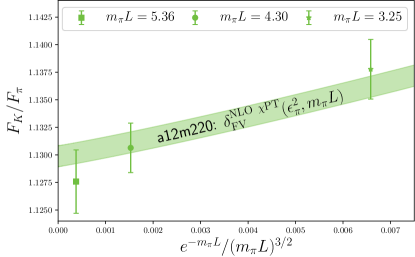
Figure 2: We compare the finite volume results on a12m220L, a12m220 and a12m220S to the predicted finite volume corrections from NLO $\chi$PT. The uncertainty band is from the full N³LO $\chi$PT extrapolation, plotted with fixed mesons masses (${\epsilon}_{P}^{2}$) and fixed lattice spacing (${\epsilon}_{a}^{2}$), determined from the a12m220L ensemble. At the one-sigma level, our data are consistent with the leading FV corrections.

III.4 N³LO corrections

The numerical dataset in this work requires us to add N³LO corrections to obtain a good fit quality. At this order, we only consider local counterterm contributions, of which there are three new continuumlike corrections and three discretization corrections. A nonunique, but complete parametrization is

$${\delta}^{\text{N${}^{3}$LO}}=({\epsilon}_{K}^{2}-{\epsilon}_{\pi}^{2})\bigg{\{}{\epsilon}_{a}^{4}A_{s}^{6}+{\epsilon}_{a}^{2}(A_{s,K}^{6}{\epsilon}_{K}^{2}+A_{s,\pi}^{6}{\epsilon}_{\pi}^{2})\\ +A_{K\pi}^{6}\,{\epsilon}_{K}^{2}{\epsilon}_{\pi}^{2}+({\epsilon}_{K}^{2}-{\epsilon}_{\pi}^{2})(A_{K}^{6}{\epsilon}_{K}^{2}+A_{\pi}^{6}{\epsilon}_{\pi}^{2})\bigg{\}}\,.$$ (58)

In principle, we could also add counterterms proportional to higher powers of ${\alpha}_{S}$ but with four lattice spacings, we would not be able to resolve the difference between the complete set of operators including all possible additional ${\alpha}_{S}$ corrections. The set of operators we do include is sufficient to parametrize the approach to the continuum limit.

IV Extrapolation Details and Uncertainty Analysis

We now carry out the extrapolation/interpolation to the physical point, which we perform in a Bayesian framework. To obtain a good fit, we must work to N³LO in the mixed chiral and continuum expansion. The results from the a06m310L ensemble drive this need, in particular, for higher-order discretization corrections to parameterize the results from all the ensembles. We will explore the impact of the a06m310L ensemble in more detail in this section. First, we discuss the values of the priors we set and the definition of the physical point.

IV.1 Prior widths for LECs

The number of additional LECs we need to determine at each order in the expansion is

order	$N_{L_{i}}$	$N_{\chi}$	$N_{a}$
NLO	1	0	0
N2LO	7	2	2
N3LO	0	3	3
Total	8	5	5

.

$N_{L_{i}}$ is the number of Gasser-Leutwyler coefficients, $N_{\chi}$ the number of counterterms associated with the continuum $\chi$PT expansion and $N_{a}$ is the number of counterterms associated with the discretization corrections. In total, there are 18 unknown LECs. While we utilize 18 ensembles in this analysis, the span of parameter space is not sufficient to constrain all the LECs without prior knowledge. In particular, the introduction of all 8 $L_{i}$ coefficients requires prior widths informed from phenomenology.

Table 5: ${\Gamma}_{i}$ coefficients that appear in the scale dependence of the $L_{i}(\mu)$. We evolve the $L_{i}(\mu)$ from the typical scale $\mu=770$ MeV, Eq. (28) to $\mu_{0}=4\pi F_{0}$, beginning with the BE14 estimates from the review Bijnens and Ecker (2014) (Table 3), using their known scale dependence Gasser and Leutwyler (1985), Eq. (59). We assign the following slightly more conservative uncertainty as a prior width in the minimization: If a value of $L_{i}$ is less than $0.5\times 10^{-3}$, we assign it a 100% uncertainty at the scale $\mu=770$ MeV; If the value is larger than $0.5\times 10^{-3}$, we assign it the larger of 0.5 or 1/3 of the mean value.

$L_{i}$	$L_{1}$	$L_{2}$	$L_{3}$	$L_{4}$	$L_{5}$	$L_{6}$	$L_{7}$	$L_{8}$
${\Gamma}_{i}$	3/32	3/16	0	1/8	3/8	11/144	0	5/48
$10^{3}L_{i}(m_{\rho})$	0.53(50)	0.81(50)	-3.1(1.0)	0.30(30)	1.01(50)	0.14(14)	-0.34(34)	0.47(47)
$10^{3}L_{i}(\mu_{0})$	0.37(50)	0.49(50)	-3.1(1.0)	0.09(30)	0.38(50)	0.01(14)	-0.34(34)	0.29(47)

In the literature, the $L_{i}$ are typically quoted at the renormalization scale $\mu_{\rho}=770$ MeV while in our work, we use the scale $\mu_{F_{0}}=4\pi F_{0}$. We can use the BE14 values of the $L_{i}$ LECs from Ref. Bijnens and Ecker (2014) and the known scale dependence Gasser and Leutwyler (1985) to convert them from $\mu_{\rho}$ to $\mu_{F_{0}}$:

$$L_{i}^{r}(\mu_{2})=L_{i}^{r}(\mu_{1})-\frac{{\Gamma}_{i}}{(4\pi)^{2}}\ln\left(\frac{\mu_{2}}{\mu_{1}}\right)\,,$$ (59)

with the values of ${\Gamma}_{i}$ listed in Table 5 for convenience. We use $F_{0}=80$ MeV, which is the value adopted by FLAG Aoki et al. (2019). We set the central value of all the $L_{i}$ with this procedure and the widths are set as described in Tab. 5.

Next, we must determine priors for the N²LO and N³LO local counterterm coefficients, $A^{n}_{K,\pi,s}$. We set the central value of all these priors to 0 and then perform a simple grid search varying the widths to find preferred values of the width, as measured by the Bayes factor. Our goal is not to optimize the width of each prior individually for each model used in the fit, but rather find a set of prior widths that is close to optimal for all models. To this end, we vary the width of the $\chi$PT LECs together at each order (N²LO, N³LO) and the discretization LECs together at each order (N²LO, N³LO) for a four-parameter search. We apply a very crude grid where the values of the widths are taken to be 2, 5, or 10.

We find taking the width of all these $A^{n}_{K,\pi,s}$ LECs equal to 2 results in good fits with near-optimal values. This provides evidence the normalization of small parameters we have chosen for ${\epsilon}_{P}^{2}$ and ${\epsilon}_{a}^{2}$, Eq. (8), is “natural” and supports the we have assumed, Eq. (9). The N²LO LECs mostly favor a width of 2 while the N³LO discretization LECs prefer 5 and the N³LO $\chi$PT LECs vary from model to model with 5 a reasonable value for all. As a result of this search, we pick as our priors

$$\tilde{A}^{4}_{K,\pi}=0\pm 2, \tilde{A}^{4}_{s}=0\pm 2,$$

$$\tilde{A}^{6}_{K,\pi}=0\pm 5, \tilde{A}^{6}_{s}=0\pm 5.$$ (60)

IV.2 Physical point

As our calculation is performed with isospin symmetric configurations and valence quarks, we must define a physical point to quote our final result. We adopt the definition of the physical point from FLAG. FLAG[2017] Aoki et al. (2016) defines the isospin symmetric pion and kaon masses to be [Eq. (16)]

$$\bar{M}_{\pi} =134.8(3)\textrm{ MeV}\,,$$

$$\bar{M}_{K} =494.2(3)\textrm{ MeV}\,.$$ (61)

The values of $F_{\pi^{+}}$ and $F_{K^{+}}$ are taken from the $N_{f}=2+1$ results from FLAG[2020] Aoki et al. (2019) (we divide the values by $\sqrt{2}$ to convert to the normalization used in this work)

$$F_{\pi^{+}}^{\rm phys} =\phantom{1}92.07(57)\textrm{ MeV}\,,$$

$$F_{K^{+}}^{\rm phys} =110.10(49)\textrm{ MeV}\,.$$ (62)

The isospin symmetric physical point is then defined by extrapolating our results to the values (for the choice $F\rightarrow F_{\pi}$)

$$({\epsilon}_{\pi}^{\rm phys})^{2} =\left(\frac{\bar{M}_{\pi}}{4\pi F_{\pi^{+}}^{\rm phys}}\right)^{2}\,,$$

$$({\epsilon}_{K}^{\rm phys})^{2} =\left(\frac{\bar{M}_{K}}{4\pi F_{\pi^{+}}^{\rm phys}}\right)^{2}\,.$$ (63)

IV.3 Model averaging procedure

Our model average is performed under a Bayesian framework following the procedure described in Kass and Raftery (1995); Chang et al. (2018). Suppose we are interested in estimating the posterior distribution of $Y=F_{K}/F_{\pi}$, ie. $P(Y|D)$ given our data $D$. To that end, we must marginalize over the different models $M_{k}$.

$$P(Y|D)=\sum_{k}P(Y|M_{k},D)P(M_{k}|D)$$ (64)

Here $P(Y|M_{k},D)$ is the distribution of $Y$ for a given model $M_{k}$ and dataset $D$, while $P(M_{k}|D)$ is the posterior distribution of $M_{k}$ given $D$. The latter can be written, per Bayes’ theorem, as

$$P(M_{k}|D)=\frac{P(D|M_{k})P(M_{k})}{\sum_{l}P(D|M_{l})P(M_{l})}\,.$$ (65)

We can be more explicit with what the latter is in the context of our fits. First, mind that we are a priori agnostic in our choice of $M_{k}$. We thus take the distribution $P(M_{k})$ to be uniform over the different models. We calculate $P(D|M_{k})$ by marginalizing over the parameters (LECs) in our fits:

$$P(D|M_{k})=\int\prod_{j}\text{d}\theta_{j}^{(k)}\,P(D|\theta_{j}^{(k)},M_{k})P(\theta_{j}^{(k)}|M_{k})\,.$$ (66)

After marginalization, $P(D|M_{k})$ is just a number. Specifically, it is the Bayes factor of $M_{k}$: $P(D|M_{k})=\exp(\texttt{logGBF})_{M_{k}}$, where logGBF is the log of the Bayes factor as reported by lsqfit Lepage (2020a). Thus

$$P(M_{k}|D)=\frac{\exp(\texttt{logGBF})_{M_{k}}}{\sum_{l=1}^{K}\exp(\texttt{logGBF})_{M_{l}}}$$ (67)

with $K$ the number of models included in our average. We emphasize that this model selection criterion not only rates the quality of the description of data but also penalizes parameters which do not improve this description. This helps rule out models which overparametrize data.

Now we can estimate the expectation value and variance of $Y$.

$$\text{E}[Y] =\sum_{k}\text{E}[Y|M_{k}]\,P(M_{k}|D)$$ (68)

$$\text{Var}[Y] =\left[\sum_{k}\text{Var}[Y|M_{k}]P(M_{k}|D)\right]$$ (69)

$$\phantom{=}+\left[\left(\sum_{k}\text{E}^{2}[Y|M_{k}]\,P(M_{k}|D)\right)-\text{E}^{2}[Y|D]\right]$$

The variance ${\rm Var}[Y]$ results from the total law of variance; the first term in brackets is known as the expected value of the process variance (which we refer to as the model averaged variance), while the latter is the variance of the hypothetical means (the root of which we refer to as the model uncertainty). After this work was completed, a similar but more thorough discussion of Bayesian model averaging in the context of lattice QCD was presented Jay and Neil (2020).

IV.4 Full analysis and uncertainty breakdown

In total, we consider 216 different models of extrapolation/interpolation to the physical point. The various choices for building a $\chi$PT or MA EFT model consist of

$$\begin{array}[]{rl}\times 2:&\textrm{$\chi$PT or MA EFT at NLO}\\ \times 3:&\textrm{use $F^{2}=\{F_{\pi}^{2},F_{\pi}F_{K},F_{K}^{2}\}$ in defining ${\epsilon}_{P}^{2}$}\\ \times 2:&\textrm{fully expanded \eqref{eq:fkfpi_fully_expanded} or ratio \eqref{eq:fkfpi_nlo_ratio} form}\\ \times 2:&\textrm{at N${}^{2}$LO, use full $\chi$PT or just counterterms}\\ \times 2:&\textrm{include or not an ${\alpha}_{S}$ term at N${}^{2}$LO}\\ \times 2:&\textrm{include or not the NLO FV corrections}\\ \times 2:&\textrm{include N${}^{3}$LO counterterms or not}\\ \hline\cr 192:&\textrm{total choices}\end{array}\,.$$

We also consider pure Taylor expansion fits with only counterterms and no log corrections. For these fits, the set of models we explore is

$$\begin{array}[]{rl}\times 2:&\textrm{work to N${}^{2}$LO or N${}^{3}$LO}\\ \times 3:&\textrm{use $F^{2}=\{F_{\pi}^{2},F_{\pi}F_{K},F_{K}^{2}\}$ in defining ${\epsilon}_{P}^{2}$}\\ \times 2:&\textrm{include or not an ${\alpha}_{S}$ term at N${}^{2}$LO}\\ \times 2:&\textrm{include or not FV corrections}\\ \hline\cr 24:&\textrm{total choices}\end{array}\,.$$

Based upon the quality of fit (gauged by the Bayesian analog to the $p$-value, $Q$, or the reduced chi square, $\chi_{\nu}^{2}$) and/or the weight determined as discussed in the previous section, we can dramatically reduce the number of models used in the final averaging procedure. First, any model which does not include the FV correction from NLO is heavily penalized. This is not surprising given the observed volume dependence on the a12m220 ensembles, Fig. 2. However, even if we remove the a12m220S ensemble from the analysis, the Taylor-expanded fits have a relative weight of $e^{-6}$ or less compared to those that have $\chi$PT form at NLO.

If we add FV corrections to the Taylor expansion fits (pure counterterm) and use all ensembles,

$$\frac{F_{K}}{F_{\pi}}=1+\bar{L}_{5}({\epsilon}_{K}^{2}-{\epsilon}_{\pi}^{2})\bigg{\{}1\\ +t_{\rm FV}\sum_{|\mathbf{n}|\neq 0}\frac{c_{n}}{m_{\pi}L|\mathbf{n}|}K_{1}(m_{\pi}L|\mathbf{n}|)\bigg{\}}+\cdots$$ (70)

they still have weights which are $\sim e^{-8}$ over the normalized model distribution and also contribute negligibly to the model average.

We observe that the fits which use the MA EFT at NLO are also penalized with a relative weight of $\sim e^{-8}$, and fits which only work to N²LO have unfavorable weights by $\sim e^{-5}$ (and are also accompanied by poor $\chi_{\nu}^{2}$ values). Cutting all of these variations reduces our final set of models to be N³LO $\chi$PT with the following variations

$$\begin{array}[]{rl}\times 3:&\textrm{use $F^{2}=\{F_{\pi}^{2},F_{\pi}F_{K},F_{K}^{2}\}$ in defining ${\epsilon}_{P}^{2}$}\\ \times 2:&\textrm{fully expanded \eqref{eq:fkfpi_fully_expanded} or ratio \eqref{eq:fkfpi_nlo_ratio} form}\\ \times 2:&\textrm{at N${}^{2}$LO, use full $\chi$PT or just counterterms}\\ \times 2:&\textrm{include or not an ${\alpha}_{S}$ term at N${}^{2}$LO}\\ \hline\cr 24:&\textrm{total choices which enter the model average}\end{array}\,.$$

The final list of models, with their corresponding weights and resulting extrapolated values to the isospin symmetric physical point, is given in Tab. 7 in Appendix A. Our final result in the isospin symmetric limit, defined as in Eq. (IV.2) and analogously for other choices of $F^{2}$, including a breakdown in terms of statistical ($s$), pion mass extrapolation ($\chi$), continuum limit ($a$), infinite volume limit ($V$), physical point (phys) and model selection ($M$) uncertainties, is as reported in Eq. (I)

$$\frac{F_{K}}{F_{\pi}} =1.1964(32)^{s}(12)^{\chi}(20)^{a}(01)^{V}(15)^{\rm phys}(12)^{M}$$

$$=1.1964(44)\,.$$

The finite volume uncertainty is assessed by removing the a12m220S ensemble from the analysis, repeating the model averaging procedure and taking the difference. The final probability distribution broken down into the three choices of $F^{2}$ is shown in Fig. 3.

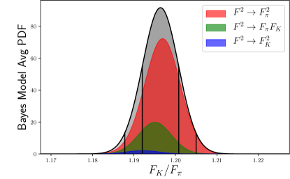
Figure 3: Final probability distribution giving rise to Eq. (I), separated into the three choices of $F^{2}=\{F_{\pi}^{2},F_{\pi}F_{K},F_{K}^{2}\}$ in the definition of the small parameters, Eq. (8). The parent “gray” distribution is the final PDF normalized to 1 when integrated.

IV.4.1 Impact of a06m310L ensemble

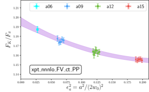
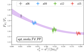
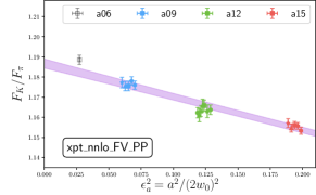
Figure 4: Left: N³LO fit to all ensembles. Middle: same fit to all ensembles excluding a06m310L. Right: representative N²LO fit to all ensembles excluding a06m310L. In all plots, the results from each ensemble are shifted to the physical values of ${\epsilon}_{\pi}^{2}$ and ${\epsilon}_{K}^{2}$ and the infinite volume limit, with only the ${\epsilon}_{a}^{2}$ dependence remaining. The labels are are explained in Appendix A; the data points at each spacing are slightly offset horizontally for visual clarity.

Next, we turn to understanding the impact of the a06m310L ensemble on our analysis. The biggest difference upon removing the a06m310L ensemble is that the data are not able to constrain the various terms contributing to the continuum extrapolation as well, particularly since there are up to three different types of scaling violations:

$$({\epsilon}_{K}^{2}-{\epsilon}_{\pi}^{2})\times\{{\epsilon}_{a}^{2},\alpha_{S}{\epsilon}_{a}^{2},{\epsilon}_{a}^{4}\}\,,$$

and thus, the statistical uncertainty of the results grows as well as the model variance, with a total uncertainty growth from $\sim 0.0044$ to $\sim 0.0057$, and the mean of the extrapolated answer moves by approximately half a standard deviation. Furthermore, N²LO fits become acceptable, though they are still grossly outweighed by the N³LO fits. Including both effects, the final model average result shifts from

$$\frac{F_{K}}{F_{\pi}}=1.1964(44)\rightarrow\frac{F_{K}}{F_{\pi}}\bigg{|}_{\rm no\ a06}=1.1941(57)\,.$$ (71)

In Fig. 4, we show the continuum extrapolation from three fits:

• Left: all ensembles, N³LO $\chi$PT with only counterterms at N²LO and N³LO and $F=F_{\pi}$;

• Middle: no a06m310L, N³LO $\chi$PT with only counterterms at N²LO and N³LO and $F=F_{\pi}$;

• Right: no a06m310L, N²LO $\chi$PT with only counterterms at N²LO and $F=F_{\pi}$.

As can be seen from the middle plot, the a15, a12 and a09 ensembles prefer contributions from both ${\epsilon}_{a}^{2}$ and ${\epsilon}_{a}^{4}$ contributions and are perfectly consistent with the result on the a06m310L ensemble. They are also consistent with an N²LO fit (no ${\epsilon}_{a}^{4}$ contributions) as can be seen in the right figure. However, the weight of the N³LO fits is still significantly greater than the N²LO fits even without the a06m310L data.

We conclude that the a06m310L ensemble is useful, but not necessary to obtain a subpercent determination of $F_{K}/F_{\pi}$ with our lattice action. A more exhaustive comparison can be performed with the analysis notebook provided with this publication.

In Fig. 5, we show the stability of our final result for various choices discussed in this section.

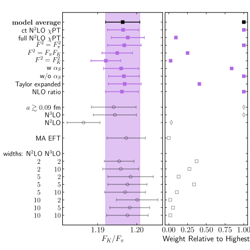
Figure 5: Stability plot of final result compared to various model choices. The black square at the top is our final answer for the isospin symmetric determination of $F_{K}/F_{\pi}$. The vertical magenta band is the uncertainty of this fit to guide the eye. The solid magenta squares are various ways of decomposing the model selection that goes into the final average. The right panel shows the relative weight with respect to the maximum logGBF value, $\exp\{\texttt{logGBF}_{i}-\texttt{logGBF}_{\rm max}\}$. Below the set of models included in the average, we show sets of analyses that are not included in the average for comparison, which are indicated with open gray symbols. First, we show the impact of excluding the a06m310L ensemble. The logGBF cannot be directly compared between these fits and the main analysis as the number of data points are not the same, so the overall normalization is different; their logGBF are shown as open diamonds. The relative logGBF between the N³LO and N²LO analysis can be compared which indicates a large preference for the N³LO analysis. We also show the MA EFT analysis, which agrees well with the main analysis. Finally, we show the results if one were to change the widths of the N²LO and N³LO priors from those chosen in Eq. (IV.1).

IV.4.2 Convergence of the chiral expansion

While the numerical analysis favors a fit function in which only counterterms are used at N²LO and higher, it is interesting to study the convergence of the chiral expansion by studying the fits which use the full $\chi$PT expression at N²LO.

In Fig. 6, we show the resulting light quark mass dependence using the N³LO extrapolation with the full N²LO $\chi$PT formula. After the analysis is performed, the results from each ensemble are shifted to the physical kaon mass point, leaving only dependence upon ${\epsilon}_{\pi}^{2}$ and ${\epsilon}_{a}^{2}$ as well as dependence upon the $\eta$ mass defined by the GMO relation. The magenta band represents the full 68% confidence interval in the continuum, infinite volume limit. The different colored curves are the mean values as a function of ${\epsilon}_{\pi}^{2}$ at the four different lattice spacings. We also show the convergence of this fit in the lower panel plot. From this convergence plot, one sees that roughly that at the physical pion mass (vertical gray line) the NLO contributions add a correction of $\sim 0.16$ compared to 1 at LO, the N²LO contributions add another $\sim 0.04$, and the N³LO corrections are not detectable by eye. The band at each order represents the sum of all terms up to that order determined from the full fit. The reduction in the uncertainty as the order is increased is due on large part to the induced correlation between the LECs at different orders through the fitting procedure.

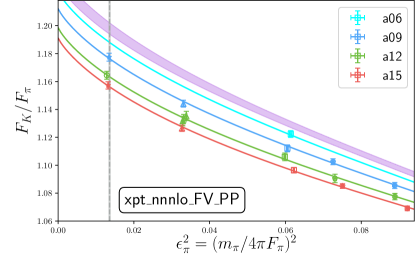
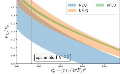
Figure 6: Sample light quark mass dependence from a $\chi$PT fit with $F=F_{\pi}$ (N²LO $\chi$PT + N³LO counterterms). Top: curves are plotted with ${\epsilon}_{K}^{2}=({\epsilon}_{K}^{\rm phys})^{2}$, at fixed ${\epsilon}_{a}^{2}$ for each lattice spacing, as a function of ${\epsilon}_{\pi}^{2}$. The magenta band is the full uncertainty in the continuum, infinite volume limit. The data points have all been shifted from the values of ${\epsilon}_{K}^{\rm latt.}$ to ${\epsilon}_{K}^{\rm phys}$ and to the infinite volume limit. Bottom: convergence of the resulting fit as a function of ${\epsilon}_{\pi}^{2}$. Each band corresponds to all contributions up to that order with the LECs determined from the full fit. The N³LO band corresponds to the continuum extrapolated band in the top figure.

In Fig. 3, we observe that the different choices of $F$ are all consistent, indicating higher-order corrections (starting at N³LO in the noncounterterm contributions) are smaller than the uncertainty in our results. It is also interesting to note that choosing $F_{\pi K}$ or $F_{K}$ is penalized by the analysis, indicating the numerical results prefer larger expansion parameters. In Tab. 6, we show the resulting $\chi$PT LECs determined in this analysis for the two choices $F=\{F_{\pi},F_{K\pi}\}$, as well as whether the ratio form of the fit is used, Eq. (24). For the Gasser-Leutwyler LECs, we evolve the values back from $\mu_{0}\rightarrow\mu_{\rho}$ for a simpler comparison with the values quoted in literature. For most of the $L_{i}$, we observe the numerical results have very little influence on the parameters as they mostly return the prior value (also listed in the table for convenience). The only LECs influenced by the fit are $L_{5}$, $L_{7}$, and $L_{8}$ with $L_{5}$ getting pulled about one sigma away from the prior value and $L_{7}$ and $L_{8}$ only shifting by a third or half of the prior width. One interesting observation from our results is that our fit prefers a value of $L_{5}$ that is noticeably smaller than the value obtained by MILC Bazavov et al. (2010a) and HPQCD Dowdall et al. (2013) and is also smaller than the BE14 result from Ref. Bijnens and Ecker (2014), although the discrepancy is still less than 2 sigma. We also note that our value of $L_{5}$ is very compatible with that determined by RBC/UKQCD with domain-wall fermions and near-physical pion masses Blum et al. (2016). Those interested in exploring this in more detail can utilize our numerical results, and if desired, extrapolation code made available with this publication.

Table 6: Resulting LECs from full N²LO $\chi$PT analysis (also including N³LO counterterms). For the Gasser-Leutwyler LECs $L_{i}$, we evolve them back to the standard scale $\mu=770$ MeV, while for the other LECs, we leave them at the scale $\mu_{0}=4\pi F_{0}\simeq 1005$ MeV.

LEC		$F^{2}=F_{\pi}^{2}$		$F^{2}=F_{\pi}F_{K}$
		ratio		ratio
$\mu=770$	prior	no	yes	no	yes
$10^{3}L_{1}$	$0.53(50)$	$0.47(49)$	$0.50(49)$	$0.45(49)$	$0.48(49)$
$10^{3}L_{2}$	$0.81(50)$	$0.77(46)$	$0.84(46)$	$0.69(44)$	$0.77(45)$
$10^{3}L_{3}$	$-3.1(1.0)$	$-3.02(85)$	$-2.84(86)$	$-3.26(81)$	$-3.05(82)$
$10^{3}L_{4}$	$0.30(30)$	$0.24(29)$	$0.14(29)$	$0.24(29)$	$0.16(29)$
$10^{3}L_{5}$	$1.01(50)$	$0.48(35)$	$0.52(34)$	$0.40(33)$	$0.47(34)$
$10^{3}L_{6}$	$0.14(14)$	$0.14(14)$	$0.14(14)$	$0.14(14)$	$0.14(14)$
$10^{3}L_{7}$	$-0.34(34)$	$-0.55(32)$	$-0.57(32)$	$-0.52(33)$	$-0.53(33)$
$10^{3}L_{8}$	$0.47(47)$	$0.30(46)$	$0.28(46)$	$0.35(46)$	$0.32(46)$
$\mu=\mu_{0}$
$A_{K}^{4}$	0(2)	$0.06(1.42)$	$0.09(1.41)$	$0.2(1.6)$	$0.2(1.5)$
$A_{\pi}^{4}$	0(2)	$2.5(1.2)$	$2.4(1.2)$	$2.0(1.3)$	$2.0(1.3)$
$A_{K\pi}^{6}$	0(5)	$2.8(4.7)$	$2.8(4.7)$	$1.9(4.7)$	$2.0(4.7)$
$A_{K}^{6}$	0(5)	$0.008(4.016)$	$0.3(4.0)$	$0.1(4.4)$	$0.2(4.4)$
$A_{p}^{6}$	0(5)	$2.6(4.0)$	$2.1(4.1)$	$2.4(4.4)$	$2.0(4.4)$

In Fig. 7, we show the impact of using the fully expanded expression, Eq. (III.1), versus the expression in which the NLO terms are kept in a ratio, Eq. (24). To simplify the comparison we restrict it to the choice $F=F_{\pi}$ and the full N²LO $\chi$PT expression. We see that fits without the ratio form are preferred, but the central value of the final result depends minimally upon this choice.

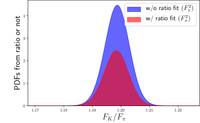
Figure 7: Comparison of fits with the fully expanded Eq. (III.1) and ratio Eq. (24) expressions, all with the choice $F=F_{\pi}$. The PDFs are taken from the parent PDF, Fig. 3 without renormalizing such that height in this figure reflects the relative weight compared to the total PDF.

In Fig. 8, we show that the results strongly favor the use of only counterterms at N²LO as opposed to the full $\chi$PT fit function at that order. We focus on the choice $F=F_{\pi}$ to simplify the comparison.

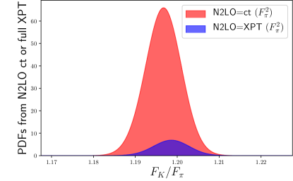
Figure 8: Comparison of N³LO $\chi$PT analysis with $F=F_{\pi}$ using the full N²LO $\chi$PT expression (smaller histogram) versus only counterterms at N²LO, Eqs. (19) and (42). As in Fig. 7, the PDFs are drawn from the parent PDF.

Our results are not sufficient to understand why the fit favors only counterterms at N²LO and higher. While the linear combination of LECs in Eq. (19) are redundant, the $L_{i}$ LECs also appear in the single-log coefficients, Eqs. (17) and (III.1) in different linear combinations. Nevertheless, we double check that the fit is not penalized for the counterterm redundancy, Eq. (19). Using the priors for $L_{i}$ from Tab. 5, we find the contribution from the Gasser-Leutwyler LECs to these N²LO counterterms, Eq. (III.1), are given by

$$L_{K}^{4}=0.3(1.3)\,, L_{\pi}^{4}=-0.64(94)\,.$$ (72)

As the $A_{P}^{4}$ terms are priored at $0(2)$, it is sufficient to rerun the analysis by simply setting $L_{P}^{4}=0$. We find this result marginally improves the Bayes factors but not statistically significantly, leaving us with the puzzle that the optimal fit is a hybrid NLO $\chi$PT plus counterterms (analytic terms) at higher orders. We note that it has been known for some time that using $\chi$PT at NLO plus purely analytic terms at NNLO and higher results in good quality extrapolation fits, at least in part because the NNLO chiral logarithms are relatively slowly varying for the range of pion masses for which the NNLO analytic terms are sizable enough to be important Aubin et al. (2004). This is discussed in more detail in the review by Bernard Bernard (2015). The MILC Collaboration no longer reports analysis with just the analytic terms at NNLO Bazavov et al. (2010a) and so it is not clear if other groups observe the same preference for counterterms only at NNLO or not.

If the Taylor expansion fits (pure counterterm) were good and favored over the $\chi$PT fits, this could be a sign that the $SU(3)$ $\chi$PT formula was failing to describe the lattice results. However, we have to include the NLO $\chi$PT expression, including its predicted (counterterm free) volume dependence to describe the numerical results. It would be nice to have the full N²LO MA EFT expression to understand why the hybrid MA EFT fits are so relatively disfavored in the analysis. There may be compensating discretization effects that cancel against those at NLO to some degree that might allow the full N²LO MA EFT to better describe the results. However, at two loops in $\chi$PT, the universality of MA EFT expressions Chen et al. (2009a) breaks down such that the MA EFT expression can no longer be “derived” from the corresponding PQ$\chi$PT one (which is known for $F_{K}/F_{\pi}$ at two loops Bijnens et al. (2004); Bijnens and Lahde (2005); Bijnens et al. (2006); Bijnens and Rössler (2015b)). It is therefore unlikely that the NNLO MA EFT expression specific to this MALQCD calculation will ever be derived, so this issue will most likely not be resolved with more clarity.

IV.5 QCD isospin breaking corrections

Finally, we discuss the correction to our result to obtain a direct determination of $F_{K^{+}}/F_{\pi^{+}}$ including strong isospin breaking corrections, but excluding QED corrections. This is the standard value quoted in the FLAG reviews Aoki et al. (2016, 2019). Our calculations, like most, are performed in the isospin symmetric limit, and therefore, the strong isospin breaking correction must be estimated, rather than having a direct determination. The optimal approach is to incorporate both QED and QCD isospin breaking corrections into the calculations such that the separation is not necessary, as was done in Ref Giusti et al. (2018) by incorporating both types of corrections through the perturbative modification of the path integral and correlation functions de Divitiis et al. (2013); Giusti et al. (2017). In this work, we have not performed these extensive computations and so we rely upon the $SU(3)$ $\chi$PT prediction to estimate the correction due to strong isospin breaking. As we have observed in Sec. IV.4, the $SU(3)$ chiral expansion behaves and converges nicely, so we expect this approximation to be reasonable.

The NLO corrections to $F_{K}$ and $F_{\pi}$ including the strong isospin breaking corrections are given by

$${\delta}F_{\pi^{\pm}}^{\rm NLO} =-\frac{\ell_{\pi^{0}}}{2}-\frac{\ell_{\pi^{\pm}}}{2}-\frac{\ell_{K^{0}}}{4}-\frac{\ell_{K^{\pm}}}{4}$$

$$\phantom{=}+4\bar{L}_{4}({\epsilon}_{\pi^{\pm}}^{2}+{\epsilon}_{K^{\pm}}^{2}+{\epsilon}_{K^{0}}^{2})+4\bar{L}_{5}{\epsilon}_{\pi^{\pm}}^{2}\,,$$

$${\delta}F_{K^{\pm}}^{\rm NLO} =-\frac{\ell_{\pi^{0}}}{8}-\frac{\ell_{\pi^{\pm}}}{4}-\frac{3\ell_{\eta}}{8}-\frac{\ell_{K^{0}}}{4}-\frac{\ell_{K^{\pm}}}{2}$$

$$\phantom{=}+\frac{1}{4}({\epsilon}_{K^{0}}^{2}-{\epsilon}_{K^{\pm}}^{2})\frac{\ell_{\eta}-\ell_{\pi^{0}}}{{\epsilon}_{\eta}^{2}-{\epsilon}_{\pi^{0}}^{2}}$$

$$\phantom{=}+4\bar{L}_{4}({\epsilon}_{\pi^{\pm}}^{2}+{\epsilon}_{K^{\pm}}^{2}+{\epsilon}_{K^{0}}^{2})+4\bar{L}_{5}{\epsilon}_{K^{\pm}}^{2}\,,$$ (73)

where we have kept explicit the contribution from each flavor of meson propagating in the loop. There are three points to note in these expressions:

1. At NLO in the $SU(3)$ chiral expansion, there are no additional LECs that describe the isospin breaking corrections beyond those that contribute to the isospin symmetric limit. Therefore, one can make a parameter-free prediction of the isospin breaking corrections using lattice results from isospin symmetric calculations, with the only assumption being that $SU(3)$ $\chi$PT converges for this observable;

2. If we expand these corrections about the isospin limit, they agree with the known results Cirigliano and Neufeld (2011), and ${\delta}F_{\pi^{\pm}}$ is free of isospin breaking corrections at this order;

3. We have used the kaon mass splitting in place of the quark mass splitting, which is exact at LO in $\chi$PT $B(m_{d}-m_{u})=(\hat{M}_{K^{0}}^{2}-\hat{M}_{K^{\pm}}^{2})$;

The estimated shift of our isospin-symmetric result to incorporate strong isospin breaking is then

$${\delta}F^{\rm iso}_{K-\pi} \equiv\frac{F_{\hat{K}^{+}}}{F_{\hat{\pi}^{+}}}-\frac{F_{K}}{F_{\pi}}$$

$$=-\frac{1}{4}(\ell_{\hat{K}^{+}}-\ell_{\bar{K}})+4\bar{L}_{5}({\epsilon}_{\hat{K}^{+}}^{2}-{\epsilon}_{\bar{K}}^{2})$$

$$\phantom{=}+\frac{1}{4}({\epsilon}_{K^{0}}^{2}-{\epsilon}_{K^{\pm}}^{2})\frac{\ell_{\eta}-\ell_{\pi^{0}}}{{\epsilon}_{\eta}^{2}-{\epsilon}_{\pi^{0}}^{2}}$$ (74)

Ref. Cirigliano and Neufeld (2011) suggested replacing $\bar{L}_{5}$ with the NLO expression equating it to the isospin symmetric $F_{K}/F_{\pi}$ which yields

$${\delta}F^{\rm iso^{\prime}}_{K-\pi}=-\frac{1}{6}\frac{{\epsilon}_{K^{0}}^{2}-{\epsilon}_{K^{\pm}}^{2}}{{\epsilon}_{\eta}^{2}-{\epsilon}_{\pi^{0}}^{2}}\bigg{[}4\left(\frac{F_{K}}{F_{\pi}}-1\right)\\ +{\epsilon}_{\bar{\pi}}^{2}\ln\left(\frac{{\epsilon}_{\bar{K}}^{2}}{{\epsilon}_{\bar{\pi}}^{2}}\right)-{\epsilon}_{\bar{K}}^{2}+{\epsilon}_{\bar{\pi}}^{2}\bigg{]}\,.$$ (75)

In this expression, we have utilized the two relations

$$\ell_{\hat{K}^{+}}-\ell_{\bar{K}} =-\frac{2}{3}\frac{{\epsilon}_{K^{0}}^{2}-{\epsilon}_{K^{\pm}}^{2}}{{\epsilon}_{\eta}^{2}-{\epsilon}_{\pi^{0}}^{2}}({\epsilon}_{\bar{K}}^{2}-{\epsilon}_{\bar{\pi}}^{2})(\ln{\epsilon}_{\bar{K}}^{2}+1)$$

$${\epsilon}_{\eta}^{2}-{\epsilon}_{\bar{\pi}}^{2} =\frac{4}{3}({\epsilon}_{\bar{K}}^{2}-{\epsilon}_{\bar{\pi}}^{2})$$ (76)

At this order, both Eqs. (IV.5) and (75) are equivalent. However, they can result in shifts that differ by more than one standard deviation. Further, the direct estimate of the strong isospin breaking corrections Carrasco et al. (2015) is larger in magnitude than either of them. Therefore, to estimate the strong isospin breaking corrections, we take the larger of the two corrections as the mean and the larger uncertainty of the two, and then add an additional 25% uncertainty for $SU(3)$ truncation errors. In Sec. IV.4.2 we observe the N²LO correction is $\sim 25\%$ of the NLO correction (while NLO is $\sim 16\%$ of LO).

In order to evaluate these expressions, we have to define the physical point with strong isospin breaking and without QED isospin breaking. We employ the values from FLAG[2017] Aoki et al. (2016) (except $\hat{M}_{\pi^{0}}=134.6(3)$ MeV):

$$\hat{M}_{\pi^{0}}=\hat{M}_{\pi^{+}} =134.8(3)\textrm{ MeV}\,,$$

$$\hat{M}_{K^{0}} =497.2(4)\textrm{ MeV}\,,$$

$$\hat{M}_{K^{+}} =491.2(5)\textrm{ MeV}\,.$$ (77)

With this definition of the physical point, we find (under the same model average as Tab. 7)

$${\delta}F^{\rm iso}_{K-\pi} =-0.00188(51)\,,$$

$${\delta}F^{\rm iso^{\prime}}_{K-\pi} =-0.00215(24)\,,$$ (78)

resulting in our estimated strong isospin breaking correction

$$\frac{F_{\hat{K}^{+}}}{F_{\hat{\pi}^{+}}}-\frac{F_{K}}{F_{\pi}} =-0.00215(72)$$ (79)

and our final result as reported in Eq. (I)

$$\frac{F_{\hat{K}^{+}}}{F_{\hat{\pi}^{+}}} =1.1942(44)(07)^{\rm iso}$$

$$=1.1942(45)\,,$$

where the first uncertainty in the first line is the combination of those in Eq. (I).

V Summary and Discussion

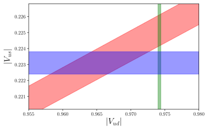
Figure 9: Result for the ratio of CKM matrix elements, $|V_{us}|/|V_{ud}|$, extracted from the ratio $F_{K}/F_{\pi}$ reported in this work (red band). The global lattice value for $|V_{us}|$ extracted from a semileptonic decay form factor, $f_{+}(0)$ Aoki et al. (2019), is shown as a horizontal blue band, while the global experimental average for $|V_{ud}|$ from nuclear beta decay Tanabashi et al. (2018) is given as a vertical green band. Note that the intersection between the red and green bands agrees well with the unitarity constraint for the CKM matrix, while the intersection between the red and blue bands shows $\sim 2\sigma$ tension.

The ratio $F_{K}/F_{\pi}$ may be used, in combination with experimental input for leptonic decay widths, to make a prediction for the ratio of CKM matrix elements, $|V_{us}|/|V_{ud}|$. Using the most recent data, Eq. (I) becomes Tanabashi et al. (2018)

$$\frac{|V_{us}|}{|V_{ud}|}\frac{F_{\hat{K}^{+}}}{F_{\hat{\pi}^{+}}}=0.2760(4)\ ,$$ (80)

where strong isospin breaking effects must be included for direct comparison with experimental data. Combining this expression with our final result, we find

$$\frac{|V_{us}|}{|V_{ud}|}=0.2311(10)\ .$$ (81)

Utilizing the current global average, $|V_{ud}|=0.97420(21)$, extracted from superallowed nuclear beta decays Tanabashi et al. (2018) results in

$$|V_{us}|=0.2251(10)\ .$$ (82)

Finally, we may use our results, combined with the value $|V_{ub}|=\left(3.94(36)\right)\times 10^{-3}$, as a test of unitarity for the CKM matrix, which states that $|V_{ud}|^{2}+|V_{us}|^{2}+|V_{ub}|^{2}=1$. From our calculation we find

$$|V_{ud}|^{2}+|V_{us}|^{2}+|V_{ub}|^{2}=0.99977(59)\ .$$ (83)

Alternatively, rather than using the experimental determination of $|V_{ud}|$ as input for our test of unitarity, we may instead use the global lattice average for $|V_{us}|=0.2231(7)$ Aoki et al. (2019), extracted via the quantity $f_{+}(0)$, the zero momentum transfer limit of a form factor relevant for the semileptonic decay $K^{0}\to\pi^{-}l\nu$. This leads to

$$|V_{ud}|^{2}+|V_{us}|^{2}+|V_{ub}|^{2}=0.9812(95)\ ,$$ (84)

leading to a roughly $2\sigma$ tension with unitarity. Our result, along with with the reported experimental results for $|V_{ud}|$ and lattice results for $|V_{us}|$, are shown in Fig. 9. One could also combine our results with the more precise average in the FLAG review which would lead to a slight reduction their reported uncertainties, but we will leave that to the FLAG Collaboration in their next update.

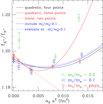
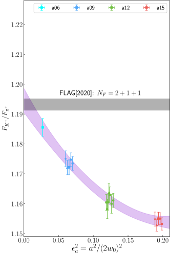
Figure 10: Comparison of the continuum extrapolation from the MILC[2014] Bazavov et al. (2014) result (LEFT) with the continuum extrapolation in the present work with the MDWF on gradient-flowed HISQ action (right). In the right plot, we also include the FLAG[2020] average value from the $N_{f}=2+1+1$ calculations Aoki et al. (2019). While the a06m310L ensemble is not necessary for us to extrapolate to a consistent value as this FLAG average (see Fig. 4), the overall size of our discretization effects are larger. This is not necessarily surprising as the HISQ action used by MILC has perturbatively removed all $\mathrm{O}(a^{2})$ corrections such that the leading scaling violations begin at $\mathrm{O}({\alpha}_{S}a^{2})$, as implied by the $x$-axis of the left plot. See Footnote 4 for a comment on the leading scaling violations Balog et al. (2009, 2010); Husung et al. (2020).

Another motivation for this work was to precisely test (below 1%) whether the action we have used for our nucleon structure calculations Berkowitz et al. (2017b); Chang et al. (2018); Berkowitz et al. (2018a) can be used to reproduce an accepted value from other lattice calculations that are known at the subpercent level. Our result provides the first subpercent cross-check of the universality of the continuum limit of this quantity with $N_{f}=2+1+1$ dynamical flavors, albeit with the same sea-quark action as used by MILC/FNAL and HPQCD Dowdall et al. (2013); Bazavov et al. (2018).

Critical in obtaining a subpercent determination of any quantity is control over the continuum extrapolation. This is relevant to our pursuit of a subpercent determination of $g_{A}$ as another calculation, utilizing many of the same HISQ ensembles but with a different valence action (clover fermions), obtains a result that is in tension with our own Bhattacharya et al. (2016); Gupta et al. (2018). While there has been speculation that this discrepancy is due to the continuum extrapolations Gupta et al. (2018), new work suggests the original work underestimated the systematic uncertainty in the correlation function analysis, and when accounted for, the tension between our results goes away Jang et al. (2020).

In either case, to obtain a subpercent determination of $g_{A}$, which is relevant for trying to shed light on the neutron lifetime discrepancy Czarnecki et al. (2018), it is important to understand the scaling violations of our lattice action. While a smooth continuum extrapolation in one observable does not guarantee such a smooth extrapolation in another, it at least provides some reassurance of a well-behaved continuum extrapolation. Furthermore, the determination of $F_{K}/F_{\pi}$ involves the same axial current that is relevant for the computation of the nucleon matrix element used to compute $g_{A}$.

Fig. 4 shows the continuum extrapolation of $F_{K}/F_{\pi}$ from our analysis. The size of the discretization effects are noticeably larger than we observed in our calculation of $g_{A}$ Chang et al. (2018). In Sec. IV.4.1, we demonstrated that, while helpful, the a06m310L ensemble is not necessary to achieve a subpercent determination of $F_{K}/F_{\pi}$. This is in contrast to the determination by MILC which requires the $a\sim 0.06$ fm (or smaller) lattice spacings to control the continuum extrapolation (though we note, the HPQCD calculation Dowdall et al. (2013), also performed on the HISQ ensembles, does not utilize the $a\sim 0.06$ fm ensembles but agrees with the MILC result). It should be noted, the MILC result does not rely on the heavier mass ensembles except to adjust for the slight mistuning of the input quark masses on their near-physical point ensembles. In Fig. 10, we compare our continuum extrapolation to that of MILC Bazavov et al. (2014).

In Ref. Bazavov et al. (2014), they also utilize the same four lattice spacings as in this work (they have subsequently improved their determination with an additional two finer lattice spacings Bazavov et al. (2018).) A strong competition between the $\mathrm{O}(a^{2})$ and $\mathrm{O}(a^{4})$ corrections was observed in that work, such that the $a\sim.06$ fm ensemble is much more instrumental for a reliable continuum extrapolation than is the case in our setup. At the same time, the overall scale of their discretization effects is much smaller than we observe in the MDWF on gradient-flowed HISQ action for this quantity. This is not entirely surprising as the HISQ action has been tuned to perturbatively remove all $\mathrm{O}(a^{2})$ corrections such that the leading corrections formally begin as $\mathrm{O}({\alpha}_{S}a^{2})$.

The analysis and supporting data for this article are openly available fkf .

Appendix A MODELS INCLUDED IN FINAL ANALYSIS

We list the models that have entered the final analysis as described in Sec. IV.4 and listed in Tab. 7. For example, the model

xpt-ratio_nnnlo_FV_alphaS_PP

indicates the model uses the continuum $\chi$PT fit function through N³LO with discretization corrections added as in Eqs. (42) and (58). The NLO contributions are kept in a ratio form, Eq. (24), and we have included the corresponding N²LO ratio correction ${\delta}_{\rm ratio}^{\text{N${}^{2}$LO}}$. The finite volume corrections have been included at NLO. The discretization terms at N²LO include the ${\alpha}_{S}{\epsilon}_{a}^{2}({\epsilon}_{K}^{2}-{\epsilon}_{\pi}^{2})$ counterterm. The renormalization scale appearing in the logs is $\mu=4\pi F_{\pi}$ as indicated by _PP, and we have included the corresponding N²LO correction ${\delta}_{F_{\pi}}^{\text{N${}^{2}$LO}}$, Eq. (III.1), to hold the actual renormalization scale fixed at $\mu_{0}=4\pi F_{0}$.

When _ct appears in the model name, the only N²LO terms that are added are from the local counterterms while all chiral log corrections are set to zero.

Table 7: List of models used in final result, as described in the text.

Model	$\chi^{2}_{\nu}$	$Q$	logGBF	weight	$F_{K}/F_{\pi}$
xpt-ratio_nnnlo_FV_ct_PP	0.847	0.645	77.728	0.273	1.1968(40)
xpt-ratio_nnnlo_FV_alphaS_ct_PP	0.843	0.650	77.551	0.229	1.1962(46)
xpt_nnnlo_FV_ct_PP	0.908	0.569	76.830	0.111	1.1974(40)
xpt_nnnlo_FV_alphaS_ct_PP	0.902	0.576	76.668	0.095	1.1966(46)
xpt-ratio_nnnlo_FV_ct_PK	1.014	0.439	76.343	0.068	1.1952(37)
xpt-ratio_nnnlo_FV_alphaS_ct_PK	1.006	0.449	76.234	0.061	1.1944(42)
xpt_nnnlo_FV_PP	0.949	0.517	75.371	0.026	1.1989(40)
xpt_nnnlo_FV_alphaS_PP	0.946	0.522	75.196	0.022	1.1983(46)
xpt_nnnlo_FV_ct_PK	1.135	0.309	75.084	0.019	1.1950(36)
xpt_nnnlo_FV_alphaS_ct_PK	1.123	0.321	75.007	0.018	1.1941(41)
xpt-ratio_nnnlo_FV_PP	1.014	0.439	74.765	0.014	1.1987(40)
xpt-ratio_nnnlo_FV_alphaS_PP	1.009	0.445	74.599	0.012	1.1980(46)
xpt_nnnlo_FV_PK	1.100	0.344	74.421	0.010	1.1969(37)
xpt_nnnlo_FV_alphaS_PK	1.093	0.352	74.306	0.009	1.1962(42)
xpt-ratio_nnnlo_FV_ct_KK	1.262	0.202	74.014	0.007	1.1920(36)
xpt-ratio_nnnlo_FV_alphaS_ct_KK	1.244	0.215	74.004	0.007	1.1912(39)
xpt-ratio_nnnlo_FV_PK	1.159	0.286	73.880	0.006	1.1967(37)
xpt-ratio_nnnlo_FV_alphaS_PK	1.150	0.295	73.780	0.005	1.1959(41)
xpt_nnnlo_FV_KK	1.288	0.184	72.757	0.002	1.1938(36)
xpt_nnnlo_FV_alphaS_KK	1.273	0.194	72.718	0.002	1.1930(40)
xpt-ratio_nnnlo_FV_KK	1.338	0.152	72.348	0.001	1.1938(36)
xpt-ratio_nnnlo_FV_alphaS_KK	1.322	0.162	72.323	0.001	1.1929(39)
xpt_nnnlo_FV_alphaS_ct_KK	1.536	0.068	71.459	0.001	1.1900(38)
xpt_nnnlo_FV_ct_KK	1.558	0.061	71.430	0.001	1.1909(35)
Bayes Model Average					1.1964(42)(12)

Appendix B NLO MIXED ACTION FORMULAS

The expression for $d\ell_{\pi}$ arises from the integral

$$d\ell_{\pi} =\int_{R}\frac{d^{d}k}{(2\pi)^{d}}\frac{i}{(k^{2}-m_{\pi}^{2})^{2}}=\frac{1+\ln(m_{\pi}^{2}/\mu^{2})}{(4\pi)^{2}}\,,$$ (85)

which has been regulated and renormalized with the standard $\chi$PT modified dimensional-regularization scheme Gasser and Leutwyler (1984). The finite volume corrections to ${\delta}\ell_{\pi}$ are given by

$${\delta}^{\rm FV}d\ell_{\pi}=\sum_{|\mathbf{n}|\neq 0}\frac{c_{n}}{(4\pi)^{2}}\bigg{[}\frac{2K_{1}(mL|\mathbf{n}|)}{mL|\mathbf{n}|}-K_{0}(mL|\mathbf{n}|)-K_{2}(mL|\mathbf{n}|)\bigg{]}$$ (86)

The expression for ${\mathcal{K}}_{\phi_{1}\phi_{2}}$ arises from the integral

$${\mathcal{K}}_{\phi_{1}\phi_{2}} =(4\pi)^{2}\int_{R}\frac{d^{d}k}{(2\pi)^{d}}\frac{i}{(k^{2}-m_{\phi_{1}}^{2})(k^{2}-m_{\phi_{2}}^{2})}=\frac{\ell_{\phi_{2}}-\ell_{\phi_{1}}}{{\epsilon}_{\phi_{2}}^{2}-{\epsilon}_{\phi_{1}}^{2}}\,.$$ (87)

Similarly, ${\mathcal{K}}_{\phi_{1}\phi_{2}}^{(2,1)}$ is given by

$${\mathcal{K}}_{\phi_{1}\phi_{2}}^{(2,1)} =\int_{R}\frac{d^{d}k}{(2\pi)^{d}}\frac{i(4\pi)^{2}(4\pi F)^{2}}{(k^{2}-m_{\phi_{1}}^{2})^{2}(k^{2}-m_{\phi_{2}}^{2})}=\frac{\ell_{\phi_{2}}-\ell_{\phi_{1}}}{({\epsilon}_{\phi_{2}}^{2}-{\epsilon}_{\phi_{1}}^{2})^{2}}-\frac{d\ell_{\phi_{1}}}{{\epsilon}_{\phi_{2}}^{2}-{\epsilon}_{\phi_{1}}^{2}}\,.$$ (88)

Finally, ${\mathcal{K}}_{\phi_{1}\phi_{2}\phi_{3}}$ is given by

$${\mathcal{K}}_{\phi_{1}\phi_{2}\phi_{3}} =\int_{R}\frac{d^{d}k}{(2\pi)^{d}}\frac{i(4\pi)^{2}(4\pi F)^{2}}{(k^{2}-m_{\phi_{1}}^{2})(k^{2}-m_{\phi_{2}}^{2})(k^{2}-m_{\phi_{3}}^{2})}$$

$$=\frac{\ell_{\phi_{1}}}{({\epsilon}_{\phi_{1}}^{2}-{\epsilon}_{\phi_{2}}^{2})({\epsilon}_{\phi_{1}}^{2}-{\epsilon}_{\phi_{3}}^{2})}+\frac{\ell_{\phi_{2}}}{({\epsilon}_{\phi_{2}}^{2}-{\epsilon}_{\phi_{1}}^{2})({\epsilon}_{\phi_{2}}^{2}-{\epsilon}_{\phi_{3}}^{2})}+\frac{\ell_{\phi_{3}}}{({\epsilon}_{\phi_{3}}^{2}-{\epsilon}_{\phi_{1}}^{2})({\epsilon}_{\phi_{3}}^{2}-{\epsilon}_{\phi_{2}}^{2})}\,.$$ (89)

In each of these expressions, the corresponding expression including FV corrections are given by replacing $\ell_{\phi}\rightarrow\ell^{\rm FV}_{\phi}$, Eq. (56).

Appendix C HYBRID MONTE CARLO FOR NEW ENSEMBLES

Table 8: Input parameters and measured acceptance rate for the new HISQ ensembles. In addition to the columns standardly reported by MILC (see Table IV of Ref. Bazavov et al. (2013)), we list the abbreviated ensemble name, the number of streams $N_{\rm stream}$, and the total number of configurations $N_{\rm cfg}$. For a given ensemble, each stream has an equal number of configurations. The gauge coupling, light, strange, and charm quark masses on each ensembles are given as well as the tadpole factor $u_{0}$ and the Naik-term added to the charm quark action ${\epsilon}_{N}$. Here $s$ denotes the total length in molecular time units (MDTU) between each saved configuration, Len. denotes the length between accept/reject steps (in MDTU), and Acc. denotes the fraction of trajectories accepted. The microstep size ${\epsilon}$ used in the HMC is provided as Len./$N_{\rm steps}$ which was input with single precision. The average acceptance rate over all streams is listed as well as the number of streams.

Ensemble	$10/g^{2}$	$am_{l}$	$am_{s}$	$am_{c}$	$u_{0}$	${\epsilon}_{N}$	$s$	Len.	${\epsilon}$	Acc.	$N_{\rm stream}$	$N_{\rm cfg}$
a15m135XL	5.80	0.002426	0.06730	0.8447	0.85535	$-$0.35892	5	0.2	0.2/150	0.631	4	2000
a09m135	6.30	0.001326	0.03636	0.4313	0.874164	$-$0.11586	6	1.5	1.5/130	0.693	2	1010
a06m310L	6.72	0.0048	0.024	0.286	0.885773	$-$0.05330	6	2.0	2.0/120	0.765	2	1000

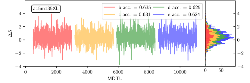
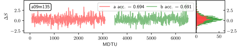
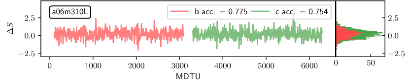
Figure 11: The $\Delta S$ values computed in the accept/reject step of the HMC versus MDTU. The different colors correspond to the different streams which are separated and shifted in MDTU for clarity.

We present various summary information for the three new ensembles used in this work, a06m310L, a15m135XL and a09m135. In Tab. 8, we list the parameters of the HISQ ensembles used in the hybrid Monte Carlo (HMC). In Fig. 11, we show the MDTU history of the ${\Delta}S$ for the three ensembles. For the a15m135XL ensemble, we reduced the trajectory length significantly compared to the a15m130 from MILC to overcome spikes in the HMC force calculations. To compensate, we lowered the acceptance rate to encourage the HMC to move around parameter space with larger jumps in an attempt to reduce the autocorrelation time. We ran 25 HMC accept/reject steps before saving a configuration for a total trajectory length of 5.

For each accept/reject step we also measure the quark-antiquark condensate $\bar{\psi}\psi$ using a stochastic estimate with 5 random sources that are averaged together. We compute it for each of the quark masses $am_{l}$, $am_{s}$, and $am_{c}$. On the a15m135XL we have measured $\bar{\psi}\psi$ only on every saved configuration for the first half of each stream, while we measured it at each accept/reject step for the second half. The integrated autocorrelation time, as well as the average and statistical errors of $\bar{\psi}\psi$, are computed using the $\Gamma$-method analysis Wolff (2004) with the Python package unew De Palma et al. (2019). We report the results in Tab. 9. In Fig. 12 we report the value of the $\bar{\psi}\psi$ on each saved configuration for the three quark masses on each ensemble.

Table 9: Average values of the quark-antiquark condensate $\bar{\psi}\psi$ with statistical errors and integrated autocorrelation times $\tau$ measured with the $\Gamma$-method analysis. Each value is averaged over all the available streams (which are all statistically compatible). The integrated autocorrelation time is reported in units of MDTU. The a15m135XL results are obtained from the second half of each stream because we have more measurements.

ensemble	$N_{\rm stream}$	$\bar{\psi}\psi_{l}$	$\tau_{l}$	$\bar{\psi}\psi_{s}$	$\tau_{s}$	$\bar{\psi}\psi_{c}$	$\tau_{c}$
a15m135XL	4	0.02390(2)	11(2)	0.08928(2)	71(26)	0.4800580(5)	$<1$
a09m135	2	0.005761(6)	9(2)	0.003935(3)	32(9)	0.3205399(5)	1.5(1)
a06m310L	2	0.006599(4)	30(8)	0.002356(2)	34(8)	0.2275664(4)	2.0(2)

$\bar{\psi}\psi_{l}$	$\bar{\psi}\psi_{s}$	$\bar{\psi}\psi_{c}$
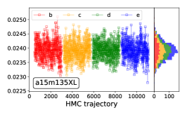
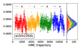
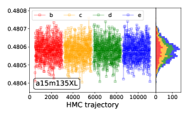
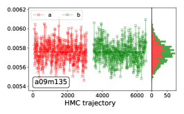
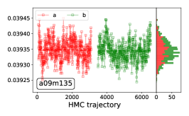
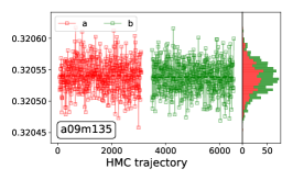
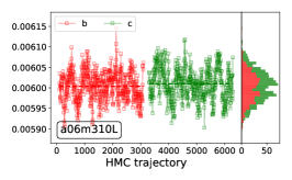
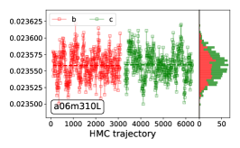
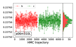
$\bar{\psi}\psi_{l}$	$\bar{\psi}\psi_{s}$	$\bar{\psi}\psi_{c}$

Figure 12: The quark-antiquark condensate on each configuration of the three ensembles. The different streams are plotted separately for clarity. The plots in each column correspond to the light, strange and charm quark masses, respectively.

Because we observe a long autocorrelation time of the $\langle\bar{\psi}_{s}\psi_{s}\rangle$ on the a15m135XL ensemble, we also studied the uncertainty on the extracted pion and kaon effective masses as a function of block size to check for possible longer autocorrelations than usual, with blocking lengths of 10, 25, and 100 MDTU (Fig. 13). We observe that these hadronic quantities have a much shorter autocorrelation time as the uncertainty is independent of ${\tau}_{b}$ and consistent with the unblocked data. On this a15m135XL ensemble, while we have generated 2000 configurations, we have only utilized 1000 in this paper (the first half from each of the four streams).

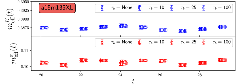
Figure 13: The effective mass in the mid- to long-time region of the kaon (top) and pion (bottom) on the a15m135XL ensemble are plotted as a function of the blocking time, ${\tau}_{b}$ in MDTU. For example, ${\tau}_{b}=10$ blocks nearest neighbor configurations while ${\tau}_{b}=100$ is blocking in groups of 20 configurations. That the uncertainty is independent of ${\tau}_{b}$ indicates the autocorrelation time for these hadronic quantities is very short.

Finally, in Tab. 10, we list the parameters of the overrelaxed stout smearing used to measure the topological charge $Q$ on each configuration Moran and Leinweber (2008) and we show the resulting $Q$ distributions in Fig. 14. While the $Q$-distribution on the a06m310L ensemble is less than ideal and the integrated autocorrelation time is long, the volume is sufficiently large ($aL=72a\simeq 4.1$ fm) that we do not anticipate any measurable impact from the poorly distributed $Q$-values, which nonetheless average to nearly 0.

Table 10: Values of the overrelaxed stout smearing parameters used to measure the topological charge $Q$ and the resulting mean ($\bar{Q}$) and width ($\sigma$) of the the distribution for each stream. The last column reports the integrated autocorrelation time in units of MDTU using the $\Gamma$-method analysis. These measurements were performed with QUDA which is now available via the su3_test test executable in the develop branch Clark et al. (2010); Babich et al. (2011).

ensemble	$\rho$	$N_{\rm step}$	$\bar{Q}_{\rm stream}(\sigma)$					$\bar{Q}_{\rm all}(\sigma)$	$\tau_{\rm all}(\sigma)$
			a	b	c	d	e
a15m135XL	$0.068$	2000	–	-10(34)	-3(35)	-2(33)	5(32)	-3(33)	15(3)
a09m135	$0.065$	2000	0.5(12.0)	2(12)	–	–	–	1(12)	18(4)
a06m310L	$0.066$	1800	–	4(12)	-1.2(7.4)	–	–	1(10)	420(198)

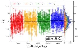
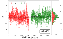
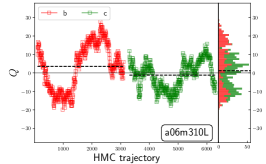
Figure 14: Distribution of topological charge $Q$ measurements on each configuration. The $Q$-values were determined by using the overrelaxed stout smearing technique outlined in Moran and Leinweber (2008) with weight parameters $\rho$ given in Tab. 10 and $\varepsilon=-0.25$. We cross-checked a sample of our stout smeared measurements with the more expensive Symanzik flow technique and saw good agreement between the two. We determined the $\rho$ parameter and the number of steps to perform on an ensemble-to-ensemble basis, i.e., for a handful of configurations per ensemble we choose a spread of $\rho$s and step numbers and observe which combination gives the best plateau. These values of $\rho$ and step number ($\varepsilon$ is always $-0.25$) are then applied to the entire ensemble.

References

- Marciano (2004) William J. Marciano, “Precise determination of —V(us)— from lattice calculations of pseudoscalar decay constants,” Phys. Rev. Lett. 93, 231803 (2004), arXiv:hep-ph/0402299 [hep-ph] .
- Aubin et al. (2004) C. Aubin, C. Bernard, Carleton E. DeTar, J. Osborn, Steven Gottlieb, E. B. Gregory, D. Toussaint, U. M. Heller, J. E. Hetrick, and R. Sugar (MILC), “Light pseudoscalar decay constants, quark masses, and low energy constants from three-flavor lattice QCD,” Phys. Rev. D70, 114501 (2004), arXiv:hep-lat/0407028 [hep-lat] .
- Decker and Finkemeier (1995) Roger Decker and Markus Finkemeier, “Short and long distance effects in the decay tau pi tau-neutrino (gamma),” Nucl. Phys. B438, 17–53 (1995), arXiv:hep-ph/9403385 [hep-ph] .
- Finkemeier (1996) Markus Finkemeier, “Radiative corrections to pi(l2) and K(l2) decays,” 2nd Workshop on Physics and Detectors for DAPHNE (DAPHNE 95) Frascati, Italy, April 4-7, 1995, Phys. Lett. B387, 391–394 (1996), arXiv:hep-ph/9505434 [hep-ph] .
- Cirigliano and Neufeld (2011) Vincenzo Cirigliano and Helmut Neufeld, “A note on isospin violation in Pl2(gamma) decays,” Phys. Lett. B700, 7–10 (2011), arXiv:1102.0563 [hep-ph] .
- Tanabashi et al. (2018) M. Tanabashi et al. (Particle Data Group), “Review of Particle Physics,” Phys. Rev. D 98, 030001 (2018).
- Davies et al. (2004) C. T. H. Davies et al. (HPQCD, UKQCD, MILC, Fermilab Lattice), “High precision lattice QCD confronts experiment,” Phys. Rev. Lett. 92, 022001 (2004), arXiv:hep-lat/0304004 [hep-lat] .
- Aoki et al. (2019) S. Aoki et al. (Flavour Lattice Averaging Group), “FLAG Review 2019,” (2019), arXiv:1902.08191 [hep-lat] .
- Carrasco et al. (2015) N. Carrasco et al., “Leptonic decay constants and with twisted-mass lattice QCD,” Phys. Rev. D91, 054507 (2015), arXiv:1411.7908 [hep-lat] .
- Frezzotti and Rossi (2004a) R. Frezzotti and G. C. Rossi, “Twisted mass lattice QCD with mass nondegenerate quarks,” Lattice hadron physics. Proceedings, 2nd Topical Workshop, LHP 2003, Cairns, Australia, July 22-30, 2003, Nucl. Phys. Proc. Suppl. 128, 193–202 (2004a), [,193(2003)], arXiv:hep-lat/0311008 [hep-lat] .
- Frezzotti and Rossi (2004b) R. Frezzotti and G. C. Rossi, “Chirally improving Wilson fermions. 1. O(a) improvement,” JHEP 08, 007 (2004b), arXiv:hep-lat/0306014 [hep-lat] .
- Dowdall et al. (2013) R. J. Dowdall, C. T. H. Davies, G. P. Lepage, and C. McNeile, “Vus from pi and K decay constants in full lattice QCD with physical u, d, s and c quarks,” Phys. Rev. D88, 074504 (2013), arXiv:1303.1670 [hep-lat] .
- Bazavov et al. (2018) A. Bazavov et al., “- and -meson leptonic decay constants from four-flavor lattice QCD,” Phys. Rev. D98, 074512 (2018), arXiv:1712.09262 [hep-lat] .
- Follana et al. (2007) E. Follana, Q. Mason, C. Davies, K. Hornbostel, G. P. Lepage, J. Shigemitsu, H. Trottier, and K. Wong (HPQCD, UKQCD), “Highly improved staggered quarks on the lattice, with applications to charm physics,” Phys. Rev. D75, 054502 (2007), arXiv:hep-lat/0610092 [hep-lat] .
- Follana et al. (2008) E. Follana, C.T.H. Davies, G.P. Lepage, and J. Shigemitsu (HPQCD, UKQCD), “High Precision determination of the pi, K, D and D(s) decay constants from lattice QCD,” Phys. Rev. Lett. 100, 062002 (2008), arXiv:0706.1726 [hep-lat] .
- Bazavov et al. (2010a) A. Bazavov et al. (MILC), “Results for light pseudoscalar mesons,” PoS LATTICE2010, 074 (2010a), arXiv:1012.0868 [hep-lat] .
- Durr et al. (2010) S. Durr, Z. Fodor, C. Hoelbling, S.D. Katz, S. Krieg, T. Kurth, L. Lellouch, T. Lippert, A. Ramos, and K.K. Szabo, “The ratio FK/Fpi in QCD,” Phys. Rev. D 81, 054507 (2010), arXiv:1001.4692 [hep-lat] .
- Blum et al. (2016) T. Blum et al. (RBC, UKQCD), “Domain wall QCD with physical quark masses,” Phys. Rev. D 93, 074505 (2016), arXiv:1411.7017 [hep-lat] .
- Dürr et al. (2017) Stephan Dürr et al., “Leptonic decay-constant ratio from lattice QCD using 2+1 clover-improved fermion flavors with 2-HEX smearing,” Phys. Rev. D 95, 054513 (2017), arXiv:1601.05998 [hep-lat] .
- Bornyakov et al. (2017) V.G. Bornyakov, R. Horsley, Y. Nakamura, H. Perlt, D. Pleiter, P.E.L. Rakow, G. Schierholz, A. Schiller, H. Stüben, and J.M. Zanotti (QCDSF–UKQCD), “Flavour breaking effects in the pseudoscalar meson decay constants,” Phys. Lett. B 767, 366–373 (2017), arXiv:1612.04798 [hep-lat] .
- Blossier et al. (2009) B. Blossier et al. (ETM), “Pseudoscalar decay constants of kaon and D-mesons from twisted mass Lattice QCD,” JHEP 07, 043 (2009), arXiv:0904.0954 [hep-lat] .
- Berkowitz et al. (2017a) E. Berkowitz, C. Bouchard, C.C Chang, M.A. Clark, B Joo, T. Kurth, C. Monahan, A. Nicholson, K. Orginos, E. Rinaldi, P. Vranas, and A. Walker-Loud, “Möbius Domain-Wall fermions on gradient-flowed dynamical HISQ ensembles,” Phys. Rev. D96, 054513 (2017a), arXiv:1701.07559 [hep-lat] .
- Bhattacharya et al. (2015) Tanmoy Bhattacharya, Vincenzo Cirigliano, Saul Cohen, Rajan Gupta, Anosh Joseph, Huey-Wen Lin, and Boram Yoon (PNDME), “Iso-vector and Iso-scalar Tensor Charges of the Nucleon from Lattice QCD,” Phys. Rev. D92, 094511 (2015), arXiv:1506.06411 [hep-lat] .
- Clark et al. (2010) M.A. Clark, R. Babich, K. Barros, R.C. Brower, and C. Rebbi, “Solving Lattice QCD systems of equations using mixed precision solvers on GPUs,” Comput.Phys.Commun. 181, 1517–1528 (2010), https://github.com/lattice/quda, arXiv:0911.3191 [hep-lat] .
- Babich et al. (2011) R. Babich, M.A. Clark, B. Joo, G. Shi, R.C. Brower, et al., “Scaling Lattice QCD beyond 100 GPUs,” (2011), arXiv:1109.2935 [hep-lat] .
- Symanzik (1983a) K. Symanzik, “Continuum Limit and Improved Action in Lattice Theories. 1. Principles and phi**4 Theory,” Nucl. Phys. B226, 187–204 (1983a).
- Symanzik (1983b) K. Symanzik, “Continuum Limit and Improved Action in Lattice Theories. 2. O(N) Nonlinear Sigma Model in Perturbation Theory,” Nucl. Phys. B226, 205–227 (1983b).
- Renner et al. (2005) Dru Bryant Renner, W. Schroers, R. Edwards, George Tamminga Fleming, Ph. Hagler, John W. Negele, K. Orginos, A. V. Pochinski, and D. Richards (LHP), “Hadronic physics with domain-wall valence and improved staggered sea quarks,” Lattice field theory. Proceedings, 22nd International Symposium, Lattice 2004, Batavia, USA, June 21-26, 2004, Nucl. Phys. Proc. Suppl. 140, 255–260 (2005), [,255(2004)], arXiv:hep-lat/0409130 [hep-lat] .
- Brower et al. (2005) Richard C. Brower, Hartmut Neff, and Kostas Orginos, “Mobius fermions: Improved domain wall chiral fermions,” Lattice field theory. Proceedings, 22nd International Symposium, Lattice 2004, Batavia, USA, June 21-26, 2004, Nucl. Phys. Proc. Suppl. 140, 686–688 (2005), [,686(2004)], arXiv:hep-lat/0409118 [hep-lat] .
- Brower et al. (2006) R. C. Brower, H. Neff, and K. Orginos, “Mobius fermions,” Hadron physics, proceedings of the Workshop on Computational Hadron Physics, University of Cyprus, Nicosia, Cyprus, 14-17 September 2005, Nucl. Phys. Proc. Suppl. 153, 191–198 (2006), arXiv:hep-lat/0511031 [hep-lat] .
- Brower et al. (2012) Richard C. Brower, Harmut Neff, and Kostas Orginos, “The möbius domain wall fermion algorithm,” (2012), arXiv:1206.5214 [hep-lat] .
- Narayanan and Neuberger (2006) R. Narayanan and H. Neuberger, “Infinite N phase transitions in continuum Wilson loop operators,” JHEP 0603, 064 (2006), arXiv:hep-th/0601210 [hep-th] .
- Lüscher and Weisz (2011) M. Lüscher and P. Weisz, “Perturbative analysis of the gradient flow in non-abelian gauge theories,” JHEP 1102, 051 (2011), arXiv:1101.0963 [hep-th] .
- Lüscher (2013) Martin Lüscher, “Chiral symmetry and the Yang–Mills gradient flow,” JHEP 1304, 123 (2013), arXiv:1302.5246 [hep-lat] .
- Lüscher (2010) Martin Lüscher, “Properties and uses of the Wilson flow in lattice QCD,” JHEP 1008, 071 (2010), arXiv:1006.4518 [hep-lat] .
- Lohmayer and Neuberger (2011) Robert Lohmayer and Herbert Neuberger, “Continuous smearing of Wilson Loops,” PoS LATTICE2011, 249 (2011), arXiv:1110.3522 [hep-lat] .
- Nicholson et al. (2018) A. Nicholson, E. Berkowitz, H. Monge-Camacho, D. Brantley, N. Garron, C. C. Chang, E. Rinaldi, M. A. Clark, B. Joó, T. Kurth, B. Tiburzi, P. Vranas, and A. Walker-Loud, “Heavy physics contributions to neutrinoless double beta decay from QCD,” Phys. Rev. Lett. 121, 172501 (2018), arXiv:1805.02634 [nucl-th] .
- Berkowitz et al. (2017b) E. Berkowitz, C. Bouchard, D. B. Brantley, C.C Chang, M.A. Clark, N. Garron, B Joó, T. Kurth, C. Monahan, H. Monge-Camacho, A. Nicholson, K. Orginos, E. Rinaldi, P. Vranas, and A. Walker-Loud, “An accurate calculation of the nucleon axial charge with lattice QCD,” (2017b), arXiv:1704.01114 [hep-lat] .
- Chang et al. (2018) C. C. Chang, A. Nicholson, E. Rinaldi, E. Berkowitz, N. Garron, D. A. Brantley, H. Monge-Camacho, C. J. Monahan, C. Bouchard, M. A. Clark, B. Joó, T. Kurth, K. Orginos, P. Vranas, and A. Walker-Loud, “A per-cent-level determination of the nucleon axial coupling from quantum chromodynamics,” Nature 558, 91–94 (2018), arXiv:1805.12130 [hep-lat] .
- Berkowitz et al. (2018a) Evan Berkowitz, M. A. Clark, A. Gambhir, K. McElvain, A. Nicholson, E. Rinalid, P. Vranas, A. Walker-Loud, C. C. Chang, B. Joó, T. Kurth, and K. Orginos, “Simulating the weak death of the neutron in a femtoscale universe with near-Exascale computing,” (2018a), arXiv:1810.01609 [hep-lat] .
- Bar et al. (2003) Oliver Bar, Gautam Rupak, and Noam Shoresh, “Simulations with different lattice Dirac operators for valence and sea quarks,” Phys. Rev. D67, 114505 (2003), arXiv:hep-lat/0210050 [hep-lat] .
- Bazavov et al. (2010b) A. Bazavov et al. (MILC), “Scaling studies of QCD with the dynamical HISQ action,” Phys. Rev. D82, 074501 (2010b), arXiv:1004.0342 [hep-lat] .
- Bazavov et al. (2013) A. Bazavov et al. (MILC), “Lattice QCD ensembles with four flavors of highly improved staggered quarks,” Phys. Rev. D87, 054505 (2013), arXiv:1212.4768 [hep-lat] .
- Kaplan (1992) David B. Kaplan, “A Method for simulating chiral fermions on the lattice,” Phys. Lett. B288, 342–347 (1992), arXiv:hep-lat/9206013 [hep-lat] .
- Shamir (1993) Yigal Shamir, “Chiral fermions from lattice boundaries,” Nucl. Phys. B406, 90–106 (1993), arXiv:hep-lat/9303005 [hep-lat] .
- Furman and Shamir (1995) Vadim Furman and Yigal Shamir, “Axial symmetries in lattice QCD with Kaplan fermions,” Nucl. Phys. B439, 54–78 (1995), arXiv:hep-lat/9405004 [hep-lat] .
- Langacker and Pagels (1973) Paul Langacker and Heinz Pagels, “Chiral perturbation theory,” Phys. Rev. D8, 4595–4619 (1973).
- Gasser and Leutwyler (1984) J. Gasser and H. Leutwyler, “Chiral Perturbation Theory to One Loop,” Annals Phys. 158, 142 (1984).
- Leutwyler (1994) H. Leutwyler, “On the foundations of chiral perturbation theory,” Annals Phys. 235, 165–203 (1994), arXiv:hep-ph/9311274 [hep-ph] .
- Sharpe and Singleton (1998) Stephen R. Sharpe and Robert L. Singleton, Jr, “Spontaneous flavor and parity breaking with Wilson fermions,” Phys. Rev. D58, 074501 (1998), arXiv:hep-lat/9804028 [hep-lat] .
- Bar et al. (2004) Oliver Bar, Gautam Rupak, and Noam Shoresh, “Chiral perturbation theory at for lattice QCD,” Phys. Rev. D70, 034508 (2004), arXiv:hep-lat/0306021 [hep-lat] .
- Bar et al. (2005) Oliver Bar, Claude Bernard, Gautam Rupak, and Noam Shoresh, “Chiral perturbation theory for staggered sea quarks and Ginsparg-Wilson valence quarks,” Phys. Rev. D72, 054502 (2005), arXiv:hep-lat/0503009 [hep-lat] .
- Tiburzi (2005) Brian C. Tiburzi, “Baryons with Ginsparg-Wilson quarks in a staggered sea,” Phys. Rev. D72, 094501 (2005), [Erratum: Phys. Rev.D79,039904(2009)], arXiv:hep-lat/0508019 [hep-lat] .
- Chen et al. (2006) Jiunn-Wei Chen, Donal O’Connell, Ruth S. Van de Water, and Andre Walker-Loud, “Ginsparg-Wilson pions scattering on a staggered sea,” Phys. Rev. D73, 074510 (2006), arXiv:hep-lat/0510024 [hep-lat] .
- Chen et al. (2007) Jiunn-Wei Chen, Donal O’Connell, and Andre Walker-Loud, “Two Meson Systems with Ginsparg-Wilson Valence Quarks,” Phys. Rev. D75, 054501 (2007), arXiv:hep-lat/0611003 [hep-lat] .
- Orginos and Walker-Loud (2008) Kostas Orginos and Andre Walker-Loud, “Mixed meson masses with domain-wall valence and staggered sea fermions,” Phys. Rev. D77, 094505 (2008), arXiv:0705.0572 [hep-lat] .
- Jiang (2007) Fu-Jiun Jiang, “Mixed Action Lattice Spacing Effects on the Nucleon Axial Charge,” (2007), arXiv:hep-lat/0703012 [hep-lat] .
- Chen et al. (2009a) Jiunn-Wei Chen, Donal O’Connell, and Andre Walker-Loud, “Universality of mixed action extrapolation formulae,” JHEP 04, 090 (2009a), arXiv:0706.0035 [hep-lat] .
- Chen et al. (2009b) Jiunn-Wei Chen, Maarten Golterman, Donal O’Connell, and Andre Walker-Loud, “Mixed Action Effective Field Theory: An Addendum,” Phys. Rev. D79, 117502 (2009b), arXiv:0905.2566 [hep-lat] .
- Blum et al. (2004) T. Blum et al., “Quenched lattice QCD with domain wall fermions and the chiral limit,” Phys. Rev. D69, 074502 (2004), arXiv:hep-lat/0007038 [hep-lat] .
- Aoki et al. (2004) Y. Aoki et al., “Domain wall fermions with improved gauge actions,” Phys. Rev. D69, 074504 (2004), arXiv:hep-lat/0211023 [hep-lat] .
- Syritsyn and Negele (2007) Sergey Syritsyn and John W. Negele, “Oscillatory terms in the domain wall transfer matrix,” Proceedings, 25th International Symposium on Lattice field theory (Lattice 2007): Regensburg, Germany, July 30-August 4, 2007, PoS LAT2007, 078 (2007), arXiv:0710.0425 [hep-lat] .
- Borsanyi et al. (2012) Szabolcs Borsanyi et al., “High-precision scale setting in lattice QCD,” JHEP 09, 010 (2012), arXiv:1203.4469 [hep-lat] .
- Amoros et al. (2000) Gabriel Amoros, Johan Bijnens, and P. Talavera, “Two point functions at two loops in three flavor chiral perturbation theory,” Nucl. Phys. B 568, 319–363 (2000), arXiv:hep-ph/9907264 .
- Ananthanarayan et al. (2017) B. Ananthanarayan, Johan Bijnens, and Shayan Ghosh, “An Analytic Analysis of the Pion Decay Constant in Three-Flavoured Chiral Perturbation Theory,” Eur. Phys. J. C 77, 497 (2017), arXiv:1703.00141 [hep-ph] .
- Ananthanarayan et al. (2018a) B. Ananthanarayan, Johan Bijnens, Samuel Friot, and Shayan Ghosh, “Analytic representations of , , and in two loop chiral perturbation theory,” Phys. Rev. D 97, 114004 (2018a), arXiv:1804.06072 [hep-ph] .
- Ananthanarayan et al. (2018b) B. Ananthanarayan, Johan Bijnens, Samuel Friot, and Shayan Ghosh, “Analytic representation of in two loop chiral perturbation theory,” Phys. Rev. D97, 091502 (2018b), arXiv:1711.11328 [hep-ph] .
- Gasser and Leutwyler (1985) J. Gasser and H. Leutwyler, “Chiral Perturbation Theory: Expansions in the Mass of the Strange Quark,” Nucl.Phys. B250, 465 (1985).
- Bijnens (2015) Johan Bijnens, “CHIRON: a package for ChPT numerical results at two loops,” Eur. Phys. J. C75, 27 (2015), arXiv:1412.0887 [hep-ph] .
- Beane et al. (2007) S. R. Beane, P. F. Bedaque, K. Orginos, and M. J. Savage (NPLQCD), “ in Full QCD with Domain Wall Valence Quarks,” Phys. Rev. D75, 094501 (2007), arXiv:hep-lat/0606023 .
- Chen and Savage (2002) Jiunn-Wei Chen and Martin J. Savage, “Baryons in partially quenched chiral perturbation theory,” Phys. Rev. D65, 094001 (2002), arXiv:hep-lat/0111050 [hep-lat] .
- Balog et al. (2009) Janos Balog, Ferenc Niedermayer, and Peter Weisz, “Logarithmic corrections to O(a**2) lattice artifacts,” Phys. Lett. B 676, 188–192 (2009), arXiv:0901.4033 [hep-lat] .
- Balog et al. (2010) Janos Balog, Ferenc Niedermayer, and Peter Weisz, “The Puzzle of apparent linear lattice artifacts in the 2d non-linear sigma-model and Symanzik’s solution,” Nucl. Phys. B 824, 563–615 (2010), arXiv:0905.1730 [hep-lat] .
- Husung et al. (2020) Nikolai Husung, Peter Marquard, and Rainer Sommer, “Asymptotic behavior of cutoff effects in Yang–Mills theory and in Wilson’s lattice QCD,” Eur. Phys. J. C 80, 200 (2020), arXiv:1912.08498 [hep-lat] .
- Gasser and Leutwyler (1987) J. Gasser and H. Leutwyler, “Light Quarks at Low Temperatures,” Phys. Lett. B184, 83–88 (1987).
- Colangelo and Haefeli (2004) Gilberto Colangelo and Christoph Haefeli, “An Asymptotic formula for the pion decay constant in a large volume,” Phys. Lett. B 590, 258–264 (2004), arXiv:hep-lat/0403025 .
- Colangelo et al. (2005) Gilberto Colangelo, Stephan Durr, and Christoph Haefeli, “Finite volume effects for meson masses and decay constants,” Nucl. Phys. B721, 136–174 (2005), arXiv:hep-lat/0503014 [hep-lat] .
- Bijnens and Rössler (2015a) Johan Bijnens and Thomas Rössler, “Finite Volume at Two-loops in Chiral Perturbation Theory,” JHEP 01, 034 (2015a), arXiv:1411.6384 [hep-lat] .
- Bijnens and Rössler (2015b) Johan Bijnens and Thomas Rössler, “Finite Volume for Three-Flavour Partially Quenched Chiral Perturbation Theory through NNLO in the Meson Sector,” JHEP 11, 097 (2015b), arXiv:1508.07238 [hep-lat] .
- Bijnens and Ecker (2014) Johan Bijnens and Gerhard Ecker, “Mesonic low-energy constants,” Ann. Rev. Nucl. Part. Sci. 64, 149–174 (2014), arXiv:1405.6488 [hep-ph] .
- Aoki et al. (2016) S. Aoki et al., “Review of lattice results concerning low-energy particle physics,” (2016), arXiv:1607.00299 [hep-lat] .
- Kass and Raftery (1995) Robert E. Kass and Adrian E. Raftery, “Bayes factors,” Journal of the American Statistical Association 90, 773–795 (1995).
- Lepage (2020a) Peter Lepage, “gplepage/lsqfit: lsqfit version 11.5.1,” (2020a), https://github.com/gplepage/lsqfit.
- Jay and Neil (2020) William I. Jay and Ethan T. Neil, “Bayesian model averaging for analysis of lattice field theory results,” (2020), arXiv:2008.01069 [stat.ME] .
- Bernard (2015) C. Bernard, “Effective Field Theories and Lattice QCD,” PoS CD15, 004 (2015), arXiv:1510.02180 [hep-ph] .
- Bijnens et al. (2004) Johan Bijnens, Niclas Danielsson, and Timo A. Lahde, “The Pseudoscalar meson mass to two loops in three-flavor partially quenched chiPT,” Phys. Rev. D 70, 111503 (2004), arXiv:hep-lat/0406017 .
- Bijnens and Lahde (2005) Johan Bijnens and Timo A. Lahde, “Decay constants of pseudoscalar mesons to two loops in three-flavor partially quenched (chi)PT,” Phys. Rev. D 71, 094502 (2005), arXiv:hep-lat/0501014 .
- Bijnens et al. (2006) Johan Bijnens, Niclas Danielsson, and Timo A. Lahde, “Three-flavor partially quenched chiral perturbation theory at NNLO for meson masses and decay constants,” Phys. Rev. D 73, 074509 (2006), arXiv:hep-lat/0602003 .
- Giusti et al. (2018) D. Giusti, V. Lubicz, G. Martinelli, C.T. Sachrajda, F. Sanfilippo, S. Simula, N. Tantalo, and C. Tarantino, “First lattice calculation of the QED corrections to leptonic decay rates,” Phys. Rev. Lett. 120, 072001 (2018), arXiv:1711.06537 [hep-lat] .
- de Divitiis et al. (2013) G.M. de Divitiis, R. Frezzotti, V. Lubicz, G. Martinelli, R. Petronzio, G.C. Rossi, F. Sanfilippo, S. Simula, and N. Tantalo (RM123), “Leading isospin breaking effects on the lattice,” Phys. Rev. D 87, 114505 (2013), arXiv:1303.4896 [hep-lat] .
- Giusti et al. (2017) D. Giusti, V. Lubicz, C. Tarantino, G. Martinelli, F. Sanfilippo, S. Simula, and N. Tantalo, “Leading isospin-breaking corrections to pion, kaon and charmed-meson masses with Twisted-Mass fermions,” Phys. Rev. D 95, 114504 (2017), arXiv:1704.06561 [hep-lat] .
- Bazavov et al. (2014) A. Bazavov et al. (Fermilab Lattice, MILC), “Charmed and light pseudoscalar meson decay constants from four-flavor lattice QCD with physical light quarks,” Phys. Rev. D90, 074509 (2014), arXiv:1407.3772 [hep-lat] .
- Bhattacharya et al. (2016) Tanmoy Bhattacharya, Vincenzo Cirigliano, Saul Cohen, Rajan Gupta, Huey-Wen Lin, and Boram Yoon, “Axial, Scalar and Tensor Charges of the Nucleon from 2+1+1-flavor Lattice QCD,” Phys. Rev. D 94, 054508 (2016), arXiv:1606.07049 [hep-lat] .
- Gupta et al. (2018) Rajan Gupta, Yong-Chull Jang, Boram Yoon, Huey-Wen Lin, Vincenzo Cirigliano, and Tanmoy Bhattacharya, “Isovector Charges of the Nucleon from 2+1+1-flavor Lattice QCD,” Phys. Rev. D 98, 034503 (2018), arXiv:1806.09006 [hep-lat] .
- Jang et al. (2020) Yong-Chull Jang, Rajan Gupta, Boram Yoon, and Tanmoy Bhattacharya, “Axial Vector Form Factors from Lattice QCD that Satisfy the PCAC Relation,” Phys. Rev. Lett. 124, 072002 (2020), arXiv:1905.06470 [hep-lat] .
- Czarnecki et al. (2018) Andrzej Czarnecki, William J. Marciano, and Alberto Sirlin, “Neutron Lifetime and Axial Coupling Connection,” Phys. Rev. Lett. 120, 202002 (2018), arXiv:1802.01804 [hep-ph] .
- (97) “Callat repository project_fkfpi,” https://github.com/callat-qcd/project_fkfpi. See also https://doi.org/10.5281/zenodo.3979560.
- Lepage (2020b) Peter Lepage, “gplepage/gvar: gvar version 11.2,” (2020b), https://github.com/gplepage/gvar.
- (99) “LALIBE: CalLat Collaboration code for lattice qcd calculations,” https://github.com/callat-qcd/lalibe.
- Edwards and Joo (2005) Robert G. Edwards and Balint Joo (SciDAC Collaboration, LHPC Collaboration, UKQCD Collaboration), “The Chroma software system for lattice QCD,” Nucl.Phys.Proc.Suppl. 140, 832 (2005), arXiv:hep-lat/0409003 [hep-lat] .
- The HDF Group (1997-NNNN) The HDF Group, “Hierarchical Data Format, version 5,” (1997-NNNN), http://www.hdfgroup.org/HDF5/.
- Kurth et al. (2015) Thorsten Kurth, Andrew Pochinsky, Abhinav Sarje, Sergey Syritsyn, and Andre Walker-Loud, “High-Performance I/O: HDF5 for Lattice QCD,” Proceedings, 32nd International Symposium on Lattice Field Theory (Lattice 2014): Brookhaven, NY, USA, June 23-28, 2014, PoS LATTICE2014, 045 (2015), arXiv:1501.06992 [hep-lat] .
- Berkowitz (2017) Evan Berkowitz, “METAQ: Bundle Supercomputing Tasks,” (2017), https://github.com/evanberkowitz/metaq, arXiv:1702.06122 [physics.comp-ph] .
- Berkowitz et al. (2018b) Evan Berkowitz, Gustav R. Jansen, Kenneth McElvain, and André Walker-Loud, “Job Management and Task Bundling,” EPJ Web Conf. 175, 09007 (2018b), arXiv:1710.01986 [hep-lat] .
- Chang et al. (2020) Chia Cheng Chang, Christopher Körber, and André Walker-Loud, “EspressoDB: A Scientific Database for Managing High-Performance Computing Workflow,” J. Open Source Softw. 5, 2007 (2020), arXiv:1912.03580 [hep-lat] .
- (106) “MILC Collaboration code for lattice qcd calculations,” https://github.com/milc-qcd/milc_qcd.
- Wolff (2004) Ulli Wolff (ALPHA), “Monte Carlo errors with less errors,” Comput. Phys. Commun. 156, 143–153 (2004), [Erratum: Comput.Phys.Commun. 176, 383 (2007)], arXiv:hep-lat/0306017 .
- De Palma et al. (2019) Barbara De Palma, Marco Erba, Luca Mantovani, and Nicola Mosco, “A Python program for the implementation of the -method for Monte Carlo simulations,” Comput. Phys. Commun. 234, 294–301 (2019), arXiv:1703.02766 [hep-lat] .
- Moran and Leinweber (2008) Peter J. Moran and Derek B. Leinweber, “Over-improved stout-link smearing,” Phys. Rev. D 77, 094501 (2008), arXiv:0801.1165 [hep-lat] .