SLIDING BIFURCATIONS IN THE MEMRISTIVE MURALI-LAKSHMANAN-CHUA CIRCUIT AND THE MEMRISTIVE DRIVEN CHUA OSCILLATOR

Abstract

In this paper we report the occurrence of sliding bifurcations admitted by the memristive Murali-Lakshmanan-Chua circuit Ishaq & Lakshmanan [2013] and the memristive driven Chua oscillator [Ishaq et al., 2011]. Both of these circuits have a flux-controlled active memristor designed by the authors in 2011, as their non-linear element. The three segment piecewise-linear characteristic of this memristor bestows on the circuits two discontinuity boundaries, dividing their phase spaces into three sub-regions. For proper choice of parameters, these circuits take on a degree of smoothness equal to one at each of their two discontinuities, thereby causing them to behave as Filippov systems. Sliding bifurcations, which are characteristic of Filippov systems, arise when the periodic orbits in each of the sub-regions, interact with the discontinuity boundaries, giving rise to many interesting dynamical phenomena. The numerical simulations are carried out after incorporating proper zero time discontinuity mapping (ZDM) corrections. These are found to agree well with the experimental observations which we report here appropriately.

1 Introduction

Among the nonlinear systems, there are large classes of systems called non-smooth systems or piecewise-smooth systems. These system are found to contain terms that are non-smooth functions of their arguments and fall outside the purview of the conventional theory of dynamical systems. Examples of such systems are electrical circuits which have switches, mechanical devices wherein components impact against each other and many control systems where continuous changes may trigger discrete actions. These systems have their phase-space divided into two or more sub-regions by the presence of what are called discontinuity boundaries. They are characterized by functions that are event driven, that is they are normally smooth but lose their smoothness at the discontinuity due to instantaneous events such as the application of a switch di Bernado et al. [2008]. Extensive studies on piecewise-smooth systems were made by Brogliato [1999, 2000], Kunze [2000], Mosekilde & Zhusubalyev [2003] and Leine & Nijmeijer [2004]. Earlier studies of these piecewise-smooth systems can also be found in the Eastern European literature, particularly the the pioneering work of Andronov et al. [2000] on non-smooth equilibrium bifurcations, Feigin’s work on C-Bifurcations Feigin [1994]; di Bernado et al. [1999], Peterka [1974] and Babitskii [1978] works on impact oscillators and Filippov [1988] work on sliding motions. All of these studies reveal that these systems posses rich and complex dynamics.

The piecewise-smooth systems, in addition to the familiar dynamical behaviours exhibited by smooth dynamical systems, are found to exhibit what are called as Discontinuity Induced Bifurcations (DIB’s). Examples of these are the border-collision bifurcations [Feigin, 1970; Nusse & Yorke, 1992], boundary equilibrium bifurcations [di Bernardo et al., 2002; Leine & Campen, 2002; Leine & Nijmeijer, 2004], grazing bifurcations Nordmark [1991]; di Bernado et al. [2001a], sliding and sticking bifurcations Feigin [1994]; di Bernado et al. [2001b, 2002, 2003], boundary intersection bifurcations Nusse & Yorke [1992] etc. The piecewise-smooth systems are classified as piecewise-smooth maps, piecewise-smooth continuous or hybrid piecewise-smooth systems based on their dependence on time. The piecewise-smooth systems having a continuous time dependence are further classified as Filippov systems or Flows based on the order of their discontinuity. Filippov systems have a discontinuity of order one [Filippov, 1964, 1988], while the flows have an order of discontinuity two or greater than two.

The memristive Murali-Lakshmanan-Chua (MMLC) circuit Ishaq & Lakshmanan [2013] and memristive driven Chua oscillator Ishaq et al. [2011] have an active flux-controlled memristor designed by the present authors in 2011 as their nonlinear element. This flux-controlled memristor, by virtue of its nonlinear characteristic, endows the circuits with two discontinuity boundaries causing them to behave as piecewise-smooth systems. In their earlier studies on the memristive MLC cirucit [Ishaq & Lakshmanan, 2013, 2017] the authors have shown that it is a continuous flow with a degree of smoothness equal to two admitting grazing bifurcations, hyperchaos, transient hyperchaos, Hopf and Neimark-Sacker bifurcations. However for proper choice of parameters, both the memristive MLC circuit and the memristive driven Chua oscillator can have a uniform discontinuity with a degree of smoothness one, thereby causing them to become Filippov systems. In this paper we report the sliding bifurcations, characteristic to Filippov systems, admitted by these memristive circuits. The paper is organized as follows. In Sec. 2, we discuss the different types of sliding bifurcations that occur in a n-dimensional system as well as the conditions for the occurrence of the same. In Sec. 3, we discuss the analog model of the memristor, its characteristic features and its experimental realization using off-the-shelf components. We then describe briefly the memristive MLC circuit, its circuit equations and their normalized forms using proper rescaling parameters. Further we consider the memristive MLC circuit as a nonsmooth system and the reformulation of the system’s equations as a set of smooth odes. We then derive the conditions for the occurrence of the sliding bifurcations, and the Zero Time Discontinuity Mapping (ZDM) corrections that are required for observing them numerically. In Sec. 4 the sliding bifurcations induced dynamics in the memristive MLC circuit is analyzed both numerically and through hardware experiments. Similar to the description of the memristive MLC circuit, in Sec. 5 we describe the memristive driven Chua oscillator, list its circuit equations and their normalized forms and reformulate the circuit as a nonsmooth system. In Sec. 6 we derive the conditions for occurrence of sliding bifurcations and the ZDM corrections required for observing them in the memristive Chua’s circuit. Further we report the crossing-sliding and grazing-sliding bifurcations occurring in it using numerical simulations as well as laboratory experiments. In Sec. 7 we present the results and conclusions.

2 Sliding Bifurcations in a General $n$-Dimensional System

Sliding bifurcations are Discontinuity Induced Bifurcations (DIB’s) arising due to the interactions between the limit cycles of a Filippov system with the boundary of a sliding region. Four types of sliding bifurcations have been identified by Feigin Feigin [1994] and were subsequently analyzed by di Bernado, Kowalczyk and others di Bernado et al. [2001b]; Kowalczyk & di Bernado [2001]; di Bernado et al. [2002, 2003] for a general $n-$dimensional system. These four sliding bifurcations are crossing-sliding bifurcations, grazing-sliding bifurcations, switching-sliding bifurcations and adding-sliding bifurcations. In this section we describe briefly the various types of sliding bifurcations, the conditions for their occurrence and the Zero Time Discontinuity Mapping (ZDM) corrections that are essential for observing these numerically.

Let us consider a piecewise-smooth continuous system having a single discontinuity boundary $\Sigma_{i,j}$. Let this discontinuity boundary divide the phase space into two sub-regions $S_{1}$ and $S_{2}$. Further let this discontinuity boundary be uniformly discontinuous in some domain $\mathcal{D}$. This means the degree of smoothness of the system is the same for all points $x\in\Sigma_{i,j}\cap\mathcal{D}$. Then this system can be written as the zero set of a smooth function $H$ such that

$$\dot{x}=\left\{\begin{array}[]{ll}F_{1}(x,\mu)\qquad\qquad\textrm{if}\qquad H(x)>0\\ F_{2}(x,\mu)\qquad\qquad\textrm{if}\qquad H(x)<0.\end{array}\right.$$ (1)

where $F_{1}(x)\neq F_{2}(x)$ at $H(x)=0$.

2.1 Types of Sliding Bifurcations

To analyze the sliding bifurcations that may occur in this general $n$-dimensional system, the state equations, Eqs. (1), are formulated using Utkin’s Equivalent Control Method (Utkin [1992]). In this method it is assumed that the system flows according to a sliding vector field, say $F_{S}$ which is the average of the two vector fields $F_{1}$ in region $S_{1}$ and $F_{2}$ in region $S_{2}$ plus a control $\beta(x)\in[-1,1]$ in the direction of the difference between the vector fields.

$$F_{s}=\dfrac{F_{1}+F_{2}}{2}+\frac{F_{2}-F_{1}}{2}\beta(x),$$ (2)

where the equivalent control is specified as

$$\beta(x)=-\dfrac{H_{x}F_{1}+H_{x}F_{2}}{H_{x}F_{2}-H_{x}F_{1}}.$$ (3)

The sliding region is given by

$$\widehat{\Sigma}:=\{x\in\Sigma:-1\leq\beta\leq 1\},$$ (4)

and its boundaries are

$$\partial\widehat{\Sigma}^{\pm}:=\{x\in\Sigma:\beta=\pm 1\}.$$ (5)

A schematic of all the sliding bifurcations are depicted in Fig. 1. Generally we assume three trajectories, say $A,\,B$ and $C$ in the neighbourhood of the switching boundary $\widehat{\Sigma}$ and study their behaviours in the sliding region bounded by $\partial\widehat{\Sigma}^{\pm}$. Of these we consider trajectory $B$ as a fiducial trajectory that crosses the sliding boundary at a precise boundary equilibrium point.

 

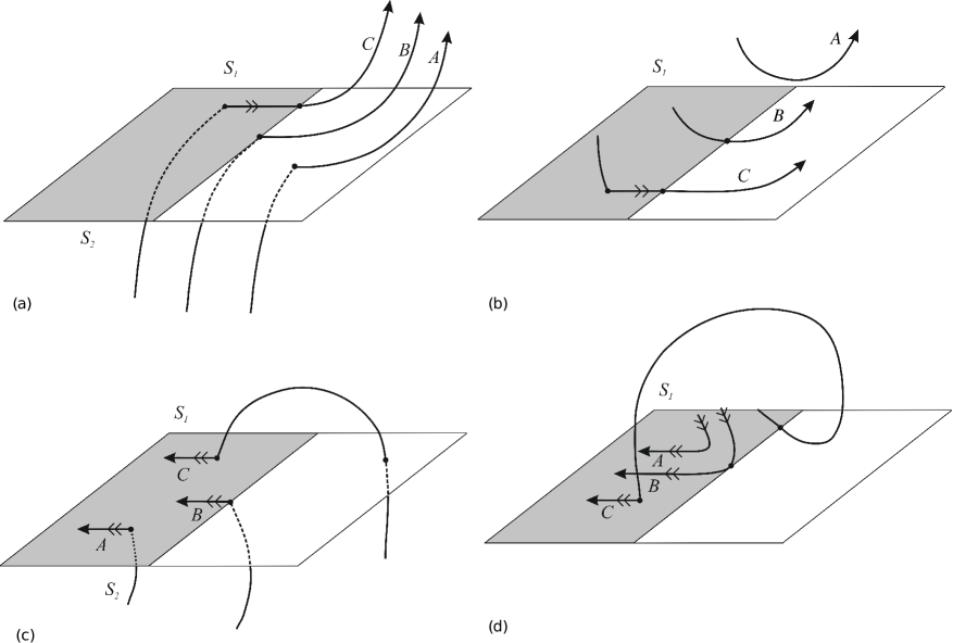
Figure 1: The four types of sliding bifurcations (a) crossing-sliding (b) grazing-sliding bifurcations (c) switching-sliding and (d) adding-sliding bifurcation.

1. Crossing-Sliding Bifurcations:
   The incidence of crossing-sliding bifurcation is shown in Fig. 1(a). Here, while all the trajectories cross the switching manifold transversely, the fiducial trajectory $B$ forms the boundary between two topologically different trajectories, with the trajectory $C$ undergoing a sliding motion in a small segment of the sliding region and trajectory $A$ not exhibiting any sliding motion at all. The trajectory $B$ therefore heralds the onset of sliding motion. This bifurcation is so called because all the trajectories incident on the switching manifold $\widehat{\Sigma}$ with zero speed, but as we move from $A\rightarrow B\rightarrow C$, we cross the sliding boundary $\partial\widehat{\Sigma}$.

2. Grazing-Sliding Bifurcations:
   Here the scenario is similar to the grazing bifurcations encountered in general piecewise-smooth continuous flows having a higher degree of smoothness, hence called as grazing-sliding bifurcations. This is shown in Fig. 1(b). Here a trajectory $A$ lying entirely in region $S_{1}$ when perturbed continuously gets converted into the trajectory $B$ which forms a point of grazing with the switching manifold. Under further perturbation, it gets converted into the trajectory $C$ which slides in a small section of sliding region, crosses the boundary $\partial\widehat{\Sigma}$ and leaves $\Sigma$ transversely.

3. Switching-Sliding Bifurcations:
   Here as we perturb the trajectory in the sequence $A\rightarrow B\rightarrow C$, we have an extra transversal crossing of $\Sigma$ or an extra switching transition. This is shown in Fig. 1(c). This is different from crossing-sliding bifurcation in that the sliding boundary $\partial\widehat{\Sigma}$ is repelling within the sliding region, whereas it is attractive in the crossing-sliding case.

4. Adding-Sliding Bifurcations:
   In this case, for a transition $A\rightarrow B\rightarrow C$, a locally uninterrupted sliding motion is transformed into two separate pieces of sliding, separated by a region of free non-sliding evolution. This causes an addition of one sliding segment to the general motion of the system under perturbation, and hence the name. This type is shown in Fig. 1(d)

2.2 Conditions for the Existence of Sliding Bifurcations

Following di Bernado et al. [2008], the conditions for the onset of various types of sliding bifurcations are given. Firstly the defining condition for all sliding motions is

$$H_{x}F_{1}(x^{*})=0.$$ (6)

This condition is to ensure that all the trajectories impinge on the switching manifold $\hat{\Sigma}$ transversely. In addition to this there is a non-degeneracy assumption valid for all sliding bifurcations

$$H_{x}F_{d}(x^{*})>0,$$ (7)

where $F_{d}=(F_{2}-F_{1})$ is the difference between the two vector fields. For crossing-sliding and grazing-sliding bifurcations we have an extra non-degeneracy condition, namely

$$H_{x}F_{1,x}F_{1}(x^{*})>0.$$ (8)

This extra non-degeneracy condition ascertains whether the boundary $\partial\widehat{\Sigma}$ is attracting or repelling to the sliding flow. For the switching-sliding bifurcation, this condition becomes

$$H_{x}F_{1,x}F_{1}(x^{*})<0,$$ (9)

while for adding-sliding bifurcation it is

$$H_{x}F_{1,x}F_{1}(x^{*})=0.$$ (10)

This condition is a defining condition for the existence of a point of tangency of the adding-sliding flow with $\partial\widehat{\Sigma}^{-}$ at the bifurcation point. Further for the adding-sliding bifurcation an extra inequality condition has to be satisfied, namely

$$H_{x}F_{1,x}^{2}F_{1}(x^{*})+H_{x}F_{1,xx}F_{1}^{2}(x^{*})<0.$$ (11)

2.3 ZDM Corrections for Sliding Bifurcations

The concept of a discontinuity map was introduced by Nordmark [1991]. This is a synthesized Poincaré map that is defined locally near the point at which a trajectory interacts with the discontinuity boundary. When composed with a global Poincaré map, say around a limit cycle, ignoring the presence of the discontinuity boundary, then one can derive a non-smooth map whose orbits describe completely the dynamics of the system. Let $\Sigma_{12}$ be a discontinuity surface that separates the phase space of a dynamical system into two regions $S_{1}$ and $S_{2}$. Let the trajectory in the sub-region $S_{1}$ be described by the flow vector $\Phi_{1}(t)$. When this trajectory intersects the discontinuity boundary $\Sigma_{12}$ and crosses over to the sub-region $S_{2}$ it will be described by the flow vector $\Phi_{2}(t)$. For periodic motions, the system trajectory crosses the discontinuity boundary $\Sigma_{12}$ multiple number of times. If the total time elapsed between successive intersections is assumed to be zero, then the mapping of the periodic orbit local to the intersecting point that translates flow vectors $\Phi_{1}(t)$ to $\Phi_{2}(t)$ is the Zero Time Discontinuity Mapping.

The Zero Time Discontinuity Map (ZDM) corrections for all the four types of sliding bifurcations for a general $n-$dimensional Filippov flow described by Eqs. (1), refer di Bernado et al. [2008], evaluated at the boundary equilibrium point $x=x^{*}$ are listed here.

1. Crossing-sliding:
   For trajectories starting in the region $S_{2}$,$(H(x)<0)$ the ZDM correction for crossing-sliding bifurcation is

   $$x\mapsto\left\{\begin{array}[]{ll}x\qquad\qquad\text{if}\,\,(H_{x}F_{1})_{x}(x-x^{*})\leq 0,\\ x+\delta_{1}\qquad\text{if}\,\,(H_{x}F_{1})_{x}(x-x^{*})>0,\\ \end{array}\right.$$ (12)

   where

   $$\delta_{1}=\dfrac{1}{2}\dfrac{[(H_{x}F_{1})_{x}(x-x^{*})]^{2}}{(H_{x}F_{2})[(H_{x}F_{1})_{x}F_{1}]}F_{d}.$$

2. Grazing-sliding:
   For trajectories starting in the region $S_{1}$,$(H(x)>0)$ the ZDM correction for grazing-sliding bifurcation is

   $$x\mapsto\left\{\begin{array}[]{ll}x\qquad\qquad\text{if}\,\,H_{x}(x-x^{*})\geq 0,\\ x+\delta_{2}\qquad\text{if}\,\,H_{x}(x-x^{*})<0,\\ \end{array}\right.$$ (13)

   where

   $$\delta_{2}=-\dfrac{H_{x}(x-x^{*})}{H_{x}F_{2}}F_{d}.$$

3. Switching-sliding:
   For trajectories starting in the region $S_{2}$,$(H(x)>0)$ the ZDM correction for switching-sliding bifurcation is

   $$x\mapsto\left\{\begin{array}[]{ll}x\qquad\qquad\text{if}\,\,(H_{x}F_{1})_{x}(x-x^{*})\leq 0,\\ x+\delta_{3}\qquad\text{if}\,\,(H_{x}F_{1})_{x}(x-x^{*})>0,\\ \end{array}\right.$$ (14)

   where

   $$\delta_{3}=\dfrac{2}{3}\dfrac{[(H_{x}F_{1})_{x}(x-x^{*})]^{3}}{(H_{x}F_{2})^{2}[(H_{x}F_{1})_{x}F_{1}]^{2}}Q,$$

   and

   $$Q=[(H_{x}F_{2})(F_{1,x}F_{d}-F_{d,x}F_{1})-(H_{x}(F_{1,x}F_{d}-F_{d,x}F_{1}))F_{d}].$$

4. Adding-sliding:
   For trajectories starting in the region $S_{1}$,$(H(x)<0)$ the ZDM correction for adding-sliding bifurcation is

   $$x\mapsto\left\{\begin{array}[]{ll}x\qquad\qquad\text{if}\,\,(H_{x}F_{1})_{x}(x-x^{*})\geq 0,\\ x+\delta_{4}\qquad\text{if}\,\,(H_{x}F_{1})_{x}(x-x^{*})<0,\\ \end{array}\right.$$ (15)

   where

   $$\delta_{4}=-\dfrac{9}{2}\dfrac{[(H_{x}F_{1})_{x}(x-x^{*})]^{2}}{(H_{x}F_{2})^{2}\{[(H_{x}F_{1})_{x}F_{1}]_{x}F_{1}\}}Q,$$

   and $Q$ is as defined earlier.

3 Memristive Murali-Lakshmanan-Chua Circuit

A memristive MLC circuit Ishaq & Lakshmanan [2013] was designed by the authors by removing the Chua’s diode and replacing it with an active flux-controlled memristor in the original Murali-Lakshmanan-Chua circuit. A memristor can be defined as any two-terminal device which exhibits a pinched hysteresis loop in the $(v-i)$ plane when driven by a bipolar periodic voltage or current excitation waveform, for any initial conditions, refer Chapter 2 by Leon O Chua in Ronald [2014]. Following the work on memrestive oscillators by Itoh & Chua [2008], a large number of researchers have proposed different models for the memristor.

3.1 Analog Memristor Model

The memristor model used in this circuit was introduced by the authors in 2011, Ishaq et al. [2011]. It has a three segment piecewise linear characteristic defined in the $(\phi-q)$ plane as shown in Fig. 2(a).

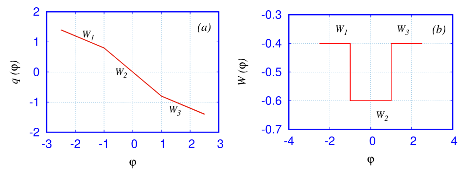
Figure 2: Characteristic of the active flux controlled memristor :(a) in the $(\phi-q(\phi))$ plane and (b) variations of the memductance $W(\phi)$ as a function of the flux $\phi$.

Mathematically the piecewise linear relationship is represented as

$$q(\phi)=W_{2}\,\phi+0.5(W_{1}-W_{2})[|\phi+1|-|\phi-1|],$$ (16)

Here the charge $q(\phi)$ is given as a function of the flux $\phi$ across the memristor. As the charge $q(\phi)$ varies, the memductance $W(\phi)=\dfrac{\partial q(\phi)}{\partial\phi}$ takes on a value $W_{2}$ for $|\phi|\leq 1$ and a value $W_{1}\equiv W_{3}$ for $|\phi|>1$. Hence this is called a flux controlled memristor. The variation in the memductance $W(\phi)$ as function of the variation of the flux $\phi$ across the memristor is shown in Fig. 2(b). Further the variations in the memductance values causes the resultant memductance $W(\phi)$ of the memristor to vary as a function of time $t$, with a low OFF state value of $W_{2}$ and high ON state value of $W_{1,3}$. This causes the current through the memristor to vary as a function of the voltage applied across it as

$$i(t)=W_{i}(\phi)v(t)\qquad\qquad\mathrm{i=1,2,3},$$ (17)

The $(v-i)$ characteristic obtained numerically by plotting the current $i(t)$ as a function of the memristor voltage $v(t)$ and is shown in Fig. 3(a). This characteristic shows a continuous switching between a set of two straight lines with slopes equal to the two memductance values $W_{2}$ and $W_{1,3}$ as the memductance $W(\phi)$ varies from a low OFF state to a high ON state and vice versa as time progresses. The corresponding experimentally observed characteristic in the $(v-i)$ plane is shown in Fig. 3(b). It is to be noted that there is a good agreement between the numerical and experimental $(v-i)$ characteristic.

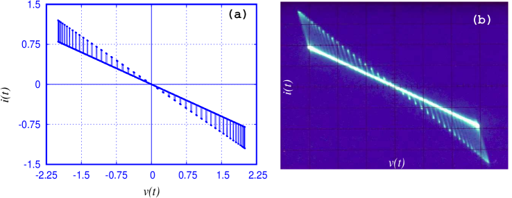
Figure 3: Memristor Characteristic (a) in the $(v(t)-i(t))$ plane obtained using numerical simulation and (b) the corresponding experimentally obtained characteristic.

The circuit realization of this memristor is given in Fig. 4.

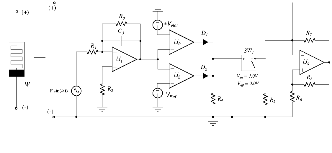
Figure 4: Analog Circuit Model of the Memristor

The analog circuit of the memrsitor shown in Fig. 4 was implemented in the laboratory using off the shelf components. Here the integrator, the window comparator as well as the negative impedance converter were implemented using TL081 operational amplifiers. The electronic switch $AD7510DJ$ was used for realizing the switching action. The reason for using TL081 is that it operates at high frequency ranges, has high slew rate and does not show hysteretic behaviour. For the integrator part of the memristor model shown in Fig. 4, the parameters were chosen as $R_{1}=10K\Omega$, $R_{2}=10K\Omega$, $R_{3}=200K\Omega$ and $C_{3}=2.2nF$. For the window comparator part the output resistance was selected as $R_{4}=10K\Omega$, while the reference voltages were fixed as $\pm 1V$. Further we had selected the linear resistances $R_{5}=3.3K\Omega$ and $R_{6}=1800\Omega$, $R_{7}=2K\Omega$ and $R_{8}=2K\Omega$ for the negative conductance. The experimental observations were made by employing a Hewlett-Packard Arbitrary Function Generator (33120A) of frequency $15$ MHz, an Agilent Mixed Storage Oscilloscope (MSO6014A) of frequency $100$ MHz and sampling rate of $2$ Giga Samples / seconds.

3.2 Experimental Realization of Memristive Murali-Lakshmanan-Chua Circuit

The experimental realization of the memristive MLC circuit is shown in Fig. 5. Using Kirchhoff’s current and voltage laws, the circuit equations can be written as a set of autonomous ordinary differential equations (ODEs), by taking the flux $\phi(t)$, voltage $v(t)$, current $i(t)$ and the time $p$ as variables as

$$\frac{d\phi}{dt} = v,$$

$$C\frac{dv}{dt} = i-W(\phi)v,$$

$$L\frac{di}{dt} = -v-Ri+F\sin(\Omega p),$$

$$\frac{dp}{dt} = 1.$$ (18)

Here $W(\phi)$ is the memductance of the memristor and is as defined in Itoh & Chua [2008],

$$W(\phi)=\frac{dq(\phi)}{d\phi}=\left\{\begin{array}[]{ll}W_{1},~{}~{}~{}\phi<1\\ W_{2},~{}~{}~{}|\phi|\leq 1\\ W_{3},~{}~{}~{}\phi>1,\end{array}\right.$$ (19)

where $W_{1}$ and $W_{3}$ are the slopes of the outer segments, such that $W_{1}=W_{3}$ and $W_{2}$ is the slope of the inner segment of the characteristic curve of the memristor respectively, refer Fig. 2(a).

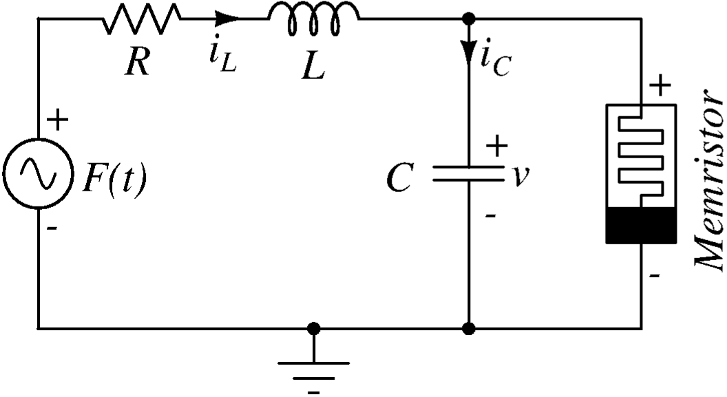
Figure 5: The experimental realization of the memristive MLC circuit, with the active flux-controlled memristor part shown by the dashed outline. The parameter values of the circuit are fixed as $L=21mH$, $R=900\Omega$, $C_{1}=10.5nF$. The frequency of the external sinusoidal forcing is fixed as $\nu_{ext}=8.288kHz$ and the amplitude is fixed as $F=770mV_{pp}$ ( peak-to-peak voltage).

These circuit equations, Eqs. (18), can be normalized as

$$\dot{x}_{1} = x_{2},$$

$$\dot{x}_{2} = x_{3}-W(x_{1})x_{2},$$

$$\dot{x}_{3} = -\beta(x_{2}+x_{3})+f\sin(\omega x_{4}),$$

$$\dot{x}_{4} = 1.$$ (20)

Here dot stands for differentiation with respect to the normalized time $\tau$ (see below) and $W(x_{1})$ is the normalized value of the memductance of the memristor, given as

$$W(x_{1})=\frac{dq(x_{1})}{dx_{1}}=\left\{\begin{array}[]{ll}a_{1},~{}~{}~{}x_{1}<1\\ a_{2},~{}~{}~{}|x_{1}|\leq 1\\ a_{3},~{}~{}~{}x_{1}>1,\end{array}\right.$$ (21)

where $a_{1}=W_{1}/G$ and $a_{3}=W_{3}/G$ are the normalized values of $W_{1}$ and $W_{3}$ with $a_{1}=a_{3}$, while $a_{2}=W_{2}/G$ is the normalized value of $W_{2}$ mentioned earlier and are negative. The rescaling parameters used for the normalization of the circuit equations are

$$x_{1}=\frac{G\phi}{C},x_{2}=v,x_{3}=\frac{i}{G},x_{4}=\frac{Gp}{C},G=\frac{1}{R},\beta=\frac{C}{LG^{2}},$$ (22)

$$\omega=\frac{\Omega C}{G}=\frac{2\pi\nu C}{G},\tau=\frac{Gt}{C},f=F\beta.$$

In our earlier work on this memristive MLC circuit, see Ishaq & Lakshmanan [2013], we reported that the addition of the memristor as the nonlinear element converts the system into a piecewise-smooth continuous flow having two discontinuous boundaries, admitting Grazing bifurcations, a type of discontinuity induced bifurcation (DIB). These grazing bifurcations were identified as the cause for the occurrence of hyperchaos, hyperchaotic beats and transient hyperchaos in this memristive MLC system. Further we reported the occurrence of discontinuity induced Hopf and Neimark-Sacker bifurcations in the same circuit Ishaq & Lakshmanan [2017]. In this paper we report the occurrence of sliding bifurcations in this circuit. These diverse dynamical behaviours prove that this simple low dimensional circuit is a robust and versatile dynamical system.

3.3 Memristive MLC Circuit as a Non-smooth System

The memristive MLC circuit is a piecewise-smooth continuous system by virtue of the discontinuous nature of its nonlinearity, namely the memristor. Referring to the memductance characteristic, we find that the memristor switches states at $x_{1}=+1$ and at $x_{1}=-1$ either from a more conductive ON state to a less conductive OFF state or vice versa. These switching states of the memristor give rise to two discontinuity boundaries or switching manifolds, $\Sigma_{1,2}$ and $\Sigma_{2,3}$ which are symmetric about the origin and are defined by the zero sets of the smooth functions $H_{i}(\mathbf{x},\mu)=C^{T}\mathbf{x}$, where $C^{T}=[1,0,0,0]$ and $\mathbf{x}=[x_{1},x_{2},x_{3},x_{4}]$, for $i=1,2$. Hence $H_{1}(\mathbf{x},\mu)=(x_{1}-x_{1}^{\ast})$, $x_{1}^{\ast}=-1$ and $H_{2}(\mathbf{x},\mu)=(x_{1}-x_{1}^{\ast})$, $x_{1}^{\ast}=+1$, respectively. Consequently the phase space $\mathcal{D}$ can be divided into three subspaces $S_{1}$, $S_{2}$ and $S_{3}$ due to the presence of the two switching manifolds. The memristive MLC circuit can now be rewritten as a set of smooth ODEs

$$\dot{\mathbf{x}}(t)=\left\{\begin{array}[]{lcccl}F_{2}(\mathbf{x},\mu),&H_{1}(\mathbf{x},\mu)\geq 0&\&&H_{2}(\mathbf{x},\mu)\leq 0,&\mathbf{x}\in S_{2},\\ &&&&\\ F_{1,3}(\mathbf{x},\mu),&H_{1}(\mathbf{x},\mu)<0&\&&H_{2}(\mathbf{x},\mu)>0,&\mathbf{x}\in S_{1,3},\end{array}\right.$$ (23)

where $\mu$ denotes the parameter dependence of the vector fields and the scalar functions. The vector fields $F_{i}$’s are

$$F_{i}(x,\mu)=\left(\begin{array}[]{cccc}0&x_{2}&0&0\\ 0&-a_{i}x_{2}&x_{3}&0\\ 0&-\beta x_{2}&-\beta x_{3}&0\\ 0&0&0&1\end{array}\right)\left(\begin{array}[]{c}1\\ 1\\ 1\\ 1\\ \end{array}\right)+\left(\begin{array}[]{c}0\\ 0\\ 1\\ 0\\ \end{array}\right)fsin(\omega x_{4}),\qquad\text{i=1,2,3},$$ (24)

where we assume $a_{1}=a_{3}$.
If the boundary equilibrium points at the two switching manifolds are taken as $X^{\ast}=\{\pm 1,x_{20},x_{30},x_{40}\}$, where $x_{20}\neq 0$, then we find that $F_{2}(x,\mu)\neq F_{1}(x,\mu)$ at $x\in\Sigma_{1,2}$ and $F_{2}(x,\mu)\neq F_{3}(x,\mu)$ at $x\in\Sigma_{2,3}$. Under these conditions the system is said to have degree of smoothness of order one, that is $r=1$, where $r$ is the order of discontinuity. Hence the memristive MLC circuit can be considered to behave as a Filippov system or a Filippov Flow capable of exhibiting sliding bifurcations.

3.4 Conditions for Sliding Bifurcations in Memristive MLC Circuit

In this section the conditions for the occurrence of sliding bifurcations in the memristive MLC circuit are derived from the general conditions for the onset of various types of sliding bifurcations given in Section 2.2. Firstly the defining condition for all sliding motions in the memristive MLC circuit is

$$x_{2}=0\qquad\qquad\textrm{for}\qquad|x_{1}|<1$$ (25)

This condition is to ensure that all the trajectories impinge on the switching manifold $\hat{\Sigma}$ transversely. In addition to this there is a non-degeneracy assumption valid for all sliding bifurcations

$$x_{2}>0\qquad\qquad\textrm{for}\qquad|x_{1}|>1$$ (26)

For crossing-sliding and grazing-sliding bifurcations we have an extra non-degeneracy condition, namely

$$(-a_{1}x_{2}+x_{3})>0\qquad\qquad\textrm{for}\qquad|x_{1}|<1$$ (27)

for the crossing-sliding case while

$$(-a_{2}x_{2}+x_{3})>0\qquad\qquad\textrm{for}\qquad|x_{1}|<1$$ (28)

for the grazing-sliding case. This extra non-degeneracy condition ascertains whether the boundary $\partial\widehat{\Sigma}$ is attracting or repelling to the sliding flow. For the switching-sliding bifurcation, this condition becomes

$$(-a_{1}x_{2}+x_{3})<0\qquad\qquad\textrm{for}\qquad|x_{1}|<1$$ (29)

while for adding-sliding bifurcation it is

$$(-a_{1}x_{2}+x_{3})=0\qquad\qquad\textrm{for}\qquad|x_{1}|<1$$ (30)

This condition is a defining condition for the existence of a point of tangency of the adding-sliding flow with $\partial\widehat{\Sigma}^{-}$ at the bifurcation point. Further for the adding-sliding bifurcation an extra inequality condition has to be satisfied, namely

$$(1-a_{1})<0.$$ (31)

As the parameter $a_{1}$ is chosen to be negative for this system, the condition given by Eq. (31), cannot be satisfied. Consequently the adding-sliding bifurcations cannot be observed in the memristive MLC circuit.

3.5 ZDM Corrections for Sliding Bifurcations in Memristive MLC Circuit

The Zero Time Discontinuity Map (ZDM) corrections for all the four types of sliding bifurcations for the memristive MLC circuit described by Eq. (23) evaluated at the boundary equilibrium points $X^{\ast}=\{\pm 1,x_{20},x_{30},x_{40}\}$, where $x_{20}\neq 0$ are derived. For an elaborate derivation of ZDM corrections for a Filippov system, refer di Bernado et al. [2008].

1. Crossing-sliding:
   For trajectories starting in the region $S_{2}$,$(H(x)<0)$ the ZDM correction for crossing-sliding bifurcation is

   $$x\mapsto\left\{\begin{array}[]{lcl}x&\text{if}&(x_{2}-x_{2}^{*})\leq 0,\\ x+\delta_{CS}&\text{if}&(x_{2}-x_{2}^{*})>0,\\ \end{array}\right.$$ (32)

   where

   $$\delta_{CS}=\left\{\begin{array}[]{llll}0,&\dfrac{1}{2}\dfrac{(a_{1}-a_{2})\epsilon^{2}}{a_{1}x_{2}},&0,&0\end{array}\right\}$$

   and $\epsilon=(x_{2}-x_{2}^{\ast})$.

2. Grazing-sliding:
   For trajectories starting in the region $S_{1}$,$(H(x)>0)$ the ZDM correction for grazing-sliding bifurcation is

   $$x\mapsto\left\{\begin{array}[]{lcl}x&\text{if}&(x_{1}-x_{1}^{*})\geq 0,\\ x-\delta_{GS}&\text{if}&(x_{1}-x_{1}^{*})<0,\\ \end{array}\right.$$ (33)

   where

   $$\delta_{GS}=\left\{\begin{array}[]{llll}0,&(a_{1}-a_{2})\epsilon,&0,&0\end{array}\right\}$$

   and $\epsilon=(x_{1}-x_{1}^{\ast})$.

3. Switching-sliding:
   For trajectories starting in the region $S_{2}$,$(H(x)>0)$ the ZDM correction for switching-sliding bifurcation is

   $$x\mapsto\left\{\begin{array}[]{lcl}x&\text{if}&(x_{2}-x_{2}^{*})\leq 0,\\ x+\delta_{SS}&\text{if}&(x_{2}-x_{2}^{*})>0.\\ \end{array}\right.$$ (34)

   where

   $$\delta_{SS}=\left\{\begin{array}[]{llll}0,&-\dfrac{2(a_{1}-a_{2})^{2}x_{2}\epsilon^{3}}{3a_{1}^{2}},&0,&0\end{array}\right\}$$

   and $\epsilon=(x_{2}-x_{2}^{\ast})$.

4. Adding-sliding:
   For trajectories starting in the region $S_{1}$,$(H(x)<0)$ the ZDM correction for adding-sliding bifurcation is

   $$x\mapsto\left\{\begin{array}[]{lcl}x&\text{if}&(x_{2}-x_{2}^{*})\leq 0,\\ x+\delta_{AS}&\text{if}&(x_{2}-x_{2}^{*})>0,\\ \end{array}\right.$$ (35)

   where

   $$\delta_{AS}=\left\{\begin{array}[]{llll}0,&\dfrac{9}{2}\dfrac{(a_{1}-a_{2})^{2}\epsilon^{2}}{(a_{1}^{2}-\beta)x_{2}},&0,&0\end{array}\right\}$$

   and $\epsilon=(x_{2}-x_{2}^{\ast})$.

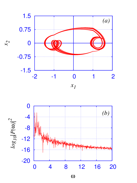
Figure 6: (a) The phase portrait of the memristive MLC circuit obtained numerically for $a_{1,3}=-0.55$, $a_{2}=-1.02$, $\omega=0.75$, $f=0.2$ and $\beta=0.99$ showing three types of sliding bifurcations admitted by the circuit. (b) The power spectrum of the $x_{2}$ variable showing quasi-periodic motion.

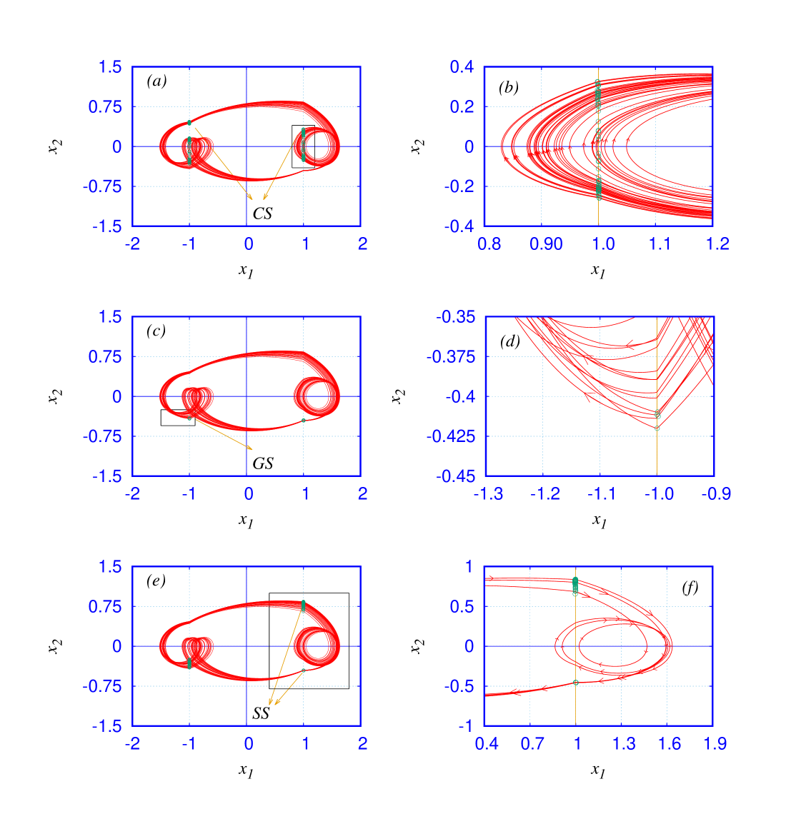
Figure 7: The phase portraits in the $(x_{1}-x_{2})$ plane capturing (a) crossing-sliding $(CS)$ bifurcations (c) grazing-sliding $GS$ bifurcations and (e) switching-sliding $SS$ bifurcations. The figures (b), (d) and (f) are the blown up portions of the same respectively, for greater clarity. The parameters are the same as mentioned in Fig. (6).

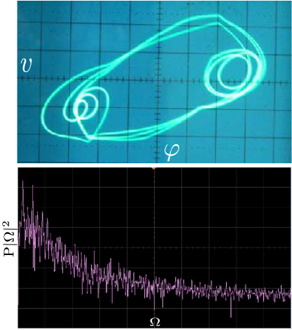
Figure 8: Figure (upper panel) is the experimental phase portrait in the $(\phi-v_{C})$ plane showing three types of sliding bifurcations of the periodic orbits and (lower panel) the power spectrum of the voltage across the capacitor $v_{c}$. The values of the memristive part of the circuit are kept constant as in Fig. 4, while the other parameters are fixed as $L=50mH$, $C=30nF$, $F=1.390VVpp$ and frequency $f=1.0744KHz$. The phase portrait corresponds well to Fig. 6 (a) while the power spectrum is in good agreement with its numerical equivalent shown in Fig. 6 (b).

4 Sliding Bifurcations Induced Dynamics of the Memristive MLC Circuit

The memristive MLC circuit admits three types of sliding bifurcations, namely the crossing-sliding, grazing-sliding and switching sliding bifurcations, for proper choice of circuit parameters. The dynamics has been studied by numerical simulation using RK4 algorithm. The normalized parameters are chosen as $a_{1}=-1.02$, $a_{2}=-0.55$, $\omega=0.75$ and $f=0.2$. Here $\beta$ is taken as the control parameter. As this control parameter is varied in the range $0.7<\beta<1.2$ we find that the circuit exhibits either one or two or all the three types of sliding bifurcations mentioned above. These are observed after the conditions for the occurrence of sliding bifurcations and the necessary Zero Discontinuity Map corrections derived above are applied to the trajectories. The sliding bifurcations so observed for $\beta=0.99$ are shown in Fig. 6(a). The power spectrum of the $x_{2}$ variable pointing to a multiple periodic behaviour is shown in Fig. 6(b).

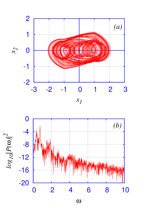
Figure 9: (a) The phase portrait of the chaotic attractor arising due to repeated sliding bifurcations occurring at the switching boundaries $\Sigma_{1,2}$ and $\Sigma_{2,3}$ for the parametric values $a_{1,3}=-0.55$, $a_{2}=-1.02$, $\omega=0.65$, $f=0.2$ and $\beta=0.97$ and (b) the power spectrum corresponding to the attractor in (a).

The figures in the plots 7(a), 7(c) and 7(e) are the phase portraits of the system for the same set of parameters mentioned above, but highlighting the particular type of sliding bifurcations. In Fig. 7(a), we find that the crossing-sliding of periodic orbits is highlighted while in 7(c) and 7(e) the grazing-sliding and switching-sliding bifurcations respectively, are clearly shown. The insets in each of these figures are expanded for greater clarity and are shown in Figs. 7(b), 7(d) and 7(f) respectively.

The experimental observations of the sliding bifurcations induced dynamics in the memristive MLC circuit are also made. For this purpose, the parametric values of the memristive part of the circuit are kept unchanged through out the study, while the other parameters are fixed as $L=50mH$, $C=30nF$, $F=1.390VVpp$ and frequency $f=1.0744KHz$. The experimental phase portrait in the $(\phi-v_{C})$ plane given in Fig. 8(a) depicts the three types of sliding bifurcations of the periodic orbits. This agrees qualitatively well with the sliding bifurcations shown in the numerical phase portrait in the $(x_{1}-x_{2})$ plane given in Fig. 6(a). The power spectrum of the voltage across the capacitor $v_{c}$, shown in Fig. 8(b) is in good agreement with its numerical equivalent shown in Fig. 6(b).

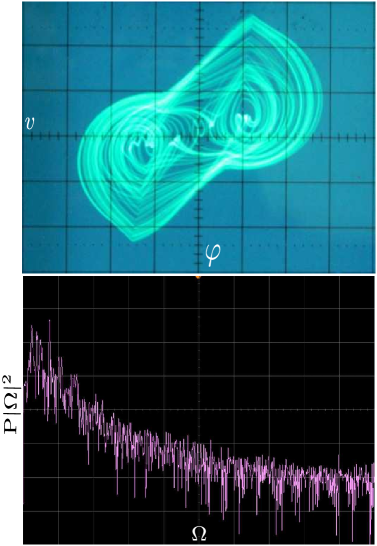
Figure 10: Figure (upper panel) showing the experimental phase portrait in the $(\phi-v_{C})$ plane exhibiting three types of sliding bifurcations of the periodic orbits and (lower panel) the power spectrum of the voltage across the capacitor $v_{c}$. The values of the memristive part of the circuit are kept constant as in Fig. 4, while the other parameters are fixed as $L=50mH$, $C=30nF$, $F=1.390VVpp$ and frequency $f=1.0744KHz$. The phase portrait corresponds well to Fig. 9 (a) while the power spectrum is in good agreement with its numerical equivalent shown in Fig. 9 (b).

4.1 Sliding Bifurcation Induced Chaos

Repeated sliding bifurcations at the discontinuity boundaries $\Sigma_{1,2}$ and $\Sigma_{2,3}$ are found to give rise to chaotic state for the memristive MLC circuit. For example for the particular choice of parameters, $a_{1,3}=-0.55$, $a_{2}=-1.02$, $\omega=0.65$, $f=0.2$ and $\beta=0.97$, the circuit is found to exhibit chaos. The phase portrait in the $(x_{1}-x_{2})$ plane and the power spectrum of the chaotic attractor arising due to sliding bifurcations are shown in Figs. 9(a) and 9(b) respectively.

The experimental phase portrait of sliding bifurcations in the $(\phi-v_{C})$ plane is shown in the upper panel of Fig. 10, while the power spectrum of the voltage across the capacitor $v_{c}$ is shown in the lower panel of Fig. 10. The values of the memristive part of the circuit are kept constant as in Fig. 4, while the other parameters are fixed as $L=50mH$, $C=30nF$, $F=1.390VVpp$ and frequency $f=1.0744KHz$. The phase portrait corresponds well to Fig. 9 (a) while the power spectrum is in good agreement with its numerical equivalent shown in Fig. 9 (b).

5 Memristive Driven Chua Oscillator

In this section, we describe the dynamics of a driven memristive Chua’s circuit. This circuit itself is obtained by modifying the driven Chua’s circuit, a fourth order non-autonomous circuit first introduced by Murali and Lakshmanan in the year 1990 Murali & Lakshmanan [1990]. The reason for selecting this circuit is that it is found to exhibit a large variety of bifurcations such as period adding, quasi-periodicity, intermittency, equal periodic bifurcations, re-emergence of double hook and double scroll attractors, hysteresis and coexistence of multiple attractors, besides the standard bifurcations. Its dynamics in the environment of a sinusoidal excitation has been extensively studied in a series of works by Murali and Lakshmanan [Murali & Lakshmanan, 1990; Lakshmanan & Murali, 1991; Murali & Lakshmanan, 1992a, c, b]. Due to its simplicity and the rich content of its nonlinear dynamical phenomena, the driven Chua’s circuit continues to evoke renewed interest by researchers in the field of non-linear electronics [Anishchenko et al., 1993; Zhu & Liu, 1997; Elwakil, 2002; Srinivasan et al., 2009]

The driven memristive Chua’s circuit is obtained by replacing the Chua’s diode in the original driven Chua’s circuit with the active flux controlled active memristor introduced by the authors in 2011, as its nonlinearity. Further the inductances in parallel in the Driven Chua’s circuit are replaced by a single equivalent inductance. The experimental realization of the driven memristive Chua’s circuit is shown in Fig. 11.

Figure 11: The experimental realization of the driven memristive Chua’s circuit.

The circuit equations, obtained by applying Kirchhoff’s laws are

$$\frac{d\phi}{dt} = v_{1},$$

$$C_{1}\frac{dv_{1}}{dt} = \frac{v_{2}-v_{1}}{R}-W(\phi)v_{1},$$

$$C_{2}\frac{dv_{2}}{dt} = \frac{v_{1}-v_{2}}{R}+i_{L},$$

$$L\frac{di_{L}}{dt} = -v_{2}-ri_{L}+F\sin(\Omega t).$$ (36)

Here $W(\phi)$ is the memductance of the memristor, defined as in Eq. (19)

The circuit equations (36) are normalized using the rescaling parameters

$$x_{1}=\frac{\phi}{RC_{2}},x_{2}=v_{1},x_{3}=v_{2},x_{4}=i_{L}R,$$

$$\alpha=\frac{C_{2}}{C_{1}},\beta=\frac{R^{2}C_{2}}{L},\gamma=\frac{RC_{2}r}{L},f=\beta F\equiv\frac{R^{2}C_{2}F}{L},\omega=\Omega RC_{2}.$$ (37)

The normalized equations so obtained are

$$\dot{x_{1}} = x_{2},$$

$$\dot{x_{2}} = \alpha\left(x_{3}-x_{2}-W(x_{1})x_{2}\right),$$

$$\dot{x_{3}} = x_{2}-x_{3}+x_{4},$$

$$\dot{x_{4}} = -\beta x_{3}-\gamma x_{4}-f\sin(\omega t).$$ (38)

Here dot stands for differentiation with respect to t. The normalized memductance of the memristor $W(x_{1})$ is the same as that defined in Eq. (21).

5.1 Memristive Driven Chua Oscillator as a Non-smooth System

Similar to the memristive MLC circuit, the driven memristive Chua’s oscillator can be considered as a piecewise-smooth system by virtue of the discontinuous nature of its nonlinearity, namely the memristor. The system possesses two discontinuity boundaries $\Sigma_{1,2}$ and $\Sigma_{2,3}$ which are symmetric about the origin, caused by the switching of the memristive states. These boundaries are defined by the zero sets of the smooth function $H_{1}(x,\mu)=(x-x^{\ast})$, $x^{\ast}=+1$ and $H_{2}=(x-x^{\ast})$, $x^{\ast}=-1$, respectively. Consequently the phase space gets divided into three sub-spaces $S_{1}$, $S_{2}$ and $S_{3}$. In the nonsmooth framework outlined earlier, the driven memristive Chua’s oscillator can be recast as a set of smooth ODE’s in each of these sub-spaces as,

$$\dot{\mathbf{x}}(t)=\left\{\begin{array}[]{lcccl}F_{2}(\mathbf{x},\mu),&H_{1}(\mathbf{x},\mu)\geq 0&\&&H_{2}(\mathbf{x},\mu)\leq 0,&\mathbf{x}\in S_{2},\\ &&&&\\ F_{1,3}(\mathbf{x},\mu),&H_{1}(\mathbf{x},\mu)<0&\&&H_{2}(\mathbf{x},\mu)>0,&\mathbf{x}\in S_{1,3},\end{array}\right.$$ (39)

where $\mu$ denotes parameter dependence of the vector fields and the scalar functions. The vector fields $F_{i}$’s are

$$F_{i}(\mathbf{x},\mu)=\left(\begin{array}[]{cccc}0&x_{2}&0&0\\ 0&-\alpha(1+a_{i})x_{2}&\alpha x_{3}&0\\ 0&x_{2}&-x_{3}&x_{4}\\ 0&0&-\beta x_{3}&-\gamma x_{4}\\ \end{array}\right)\left(\begin{array}[]{c}1\\ 1\\ 1\\ 1\\ \end{array}\right)+\left(\begin{array}[]{c}0\\ 0\\ 0\\ 1\\ \end{array}\right)fsin(\omega t),\qquad\text{i=1,2,3}$$ (40)

with the assumption that $a_{1}=a_{3}$.

6 Sliding Bifurcations in Memristive Driven Chua Oscillator

In this section we report the simultaneous occurrence of two types of sliding bifurcations in the driven memristive Chua’s circuit, for the same set of circuit parameters. To analyze these sliding bifurcations, the normalized state equations for the driven memristive Chua’s circuit, Eqs. (39), are reformulated using Utkin’s Equivalent Control Method, refer Utkin [1992], as

$$F_{S}=\dfrac{F_{1}+F_{2}}{2}+\frac{F_{2}-F_{1}}{2}\beta(x).$$ (41)

Here it is assumed that the system flows according to a sliding vector field, $F_{S}$, which is the average of the two vector fields $F_{1}$ in region $S_{1}$ and $F_{2}$ in region $S_{2}$ plus an equivalent control $\beta(x)\in[-1,1]$ specified as

$$\beta(x)=-\dfrac{H_{x}F_{1}+H_{x}F_{2}}{H_{x}F_{2}-H_{x}F_{1}},$$ (42)

in the direction of the difference between the vector fields. The sliding region is given by

$$\widehat{\Sigma}:=\{x\in\Sigma:-1\leq\beta\leq 1\},$$ (43)

and its boundaries are

$$\partial\widehat{\Sigma}^{\pm}:=\{x\in\Sigma:\beta=\pm 1\}.$$ (44)

The vector fields $F_{i}$’s, are the same as defined in Eq. (40)

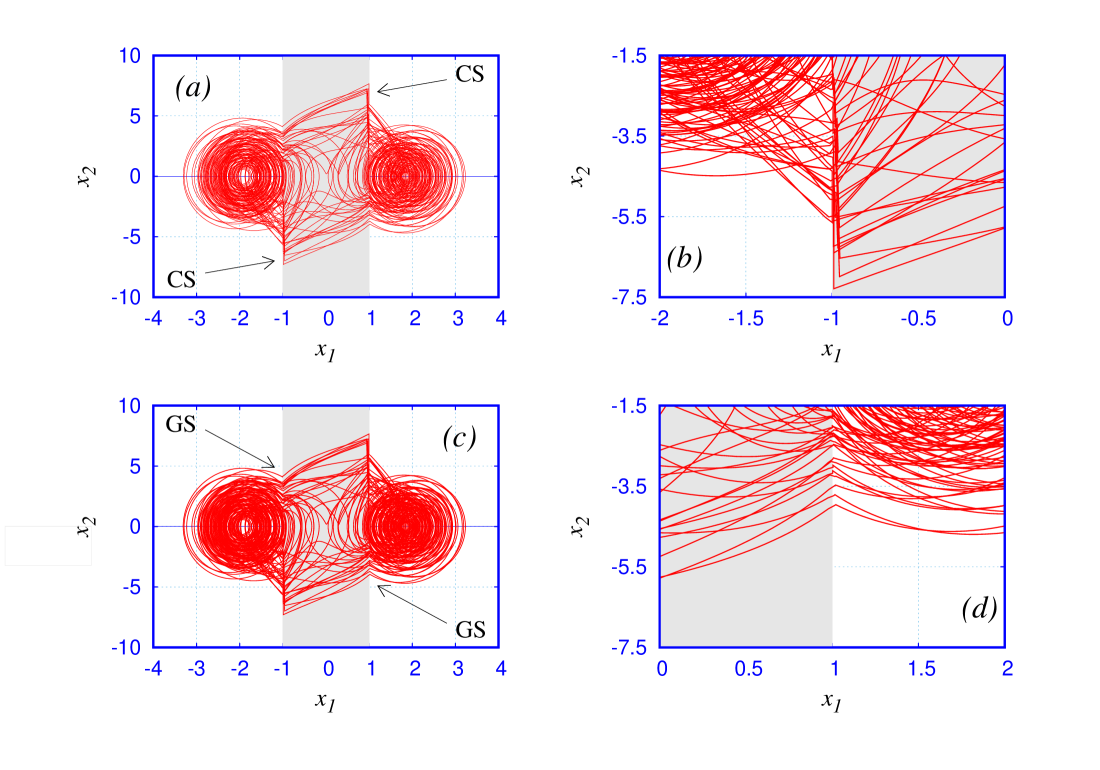
Figure 12: The phase portrait in the $(x_{1}-x_{2})$ plane for $a_{1,3}=-0.68$, $a_{2}=-1.27$, $\beta=16$ and $\gamma=0.035$ ,$\omega=0.35$, $f=0.125$ and $\alpha=9.3$. The arrows show (a) the crossing-sliding $CS$ interactions of the trajectories and (c) the grazing-sliding $GS$ with the switching manifolds $\Sigma_{1,2}$ and $\Sigma_{2,3}$. Figs. (b) and (d) are the enlargements of the corresponding phase portraits included here for greater clarity.

6.1 Crossing-Sliding and Grazing-Sliding Bifurcations

Based on the conditions for the occurrence of various types of sliding bifurcations, refer Eqs. (6)-(11), the conditions for observing the same in the memristive driven Chua oscillator are derived. Using these, we find that the driven memristive Chua’s circuit exhibits crossing-sliding bifurcations and grazing-sliding bifurcations when the trajectories cross the switching manifolds $\Sigma_{i,j}$’s a multiple number of times as the dynamics unfolds. To our knowledge, it is for the first time that both types of sliding bifurcations are undergone by the system for the same set of parameters. These sliding bifurcations lead to chaotic behaviours.
The crossing-sliding bifurcations are found to occur when some of the trajectories that cross the switching manifolds $\Sigma_{i,j}$’s, for $i,j=1,2$ are incident within the sliding regions $\widehat{\Sigma}_{i,j}$. In these sliding regions the trajectories show a sliding motion for a short interval of time and are governed by the sliding vector field $F_{S}$ before they reach the sliding boundaries $\partial\widehat{\Sigma}^{\pm}$ and move over to regions governed by either $F_{2}$ or $F_{1,3}$.

The grazing-sliding bifurcations are similar to the grazing bifurcations encountered in general piecewise-smooth continuous flows having a higher degree of smoothness. However, these bifurcations differ from pure grazing bifurcations in that, some of the trajectories that are incident on the sliding regions $\widehat{\Sigma}_{i,j}$, exhibit sliding motion in small segments of these regions before they cross the sliding boundaries $\partial\widehat{\Sigma}^{\pm}$ and leave the switching manifolds $\Sigma_{i,j}$ transversely.
The conditions for the onset of crossing sliding and grazing sliding bifurcations in the memristive driven Chua oscillator are given below.
The defining condition for all sliding motions in the driven memristive Chua’s circuit is

$$x_{2}^{*}=0,\qquad\qquad\textrm{for}\qquad|x_{1}|<1.$$ (45)

This condition is to ensure that all the trajectories impinge on the switching manifolds $\widehat{\Sigma}_{1,2}$ and $\widehat{\Sigma}_{2,3}$ transversely. The non-degeneracy assumption valid for all sliding bifurcations in this system takes the form,

$$x_{2}^{*}>0,\qquad\qquad\textrm{for}\qquad|x_{1}|>1.$$ (46)

The extra non-degeneracy condition applicable to crossing-sliding bifurcations becomes

$$\alpha[x_{3}-(1+a_{2})x_{2}]>0,\qquad\qquad\textrm{for}\qquad-1<x_{1}<1,$$ (47)

while for grazing-sliding bifurcations, we have

$$\alpha[x_{3}-(1+a_{2})x_{2}]>0,\qquad\qquad\textrm{for}\qquad|x_{1}|>1.$$ (48)

These extra non-degeneracy conditions ascertain whether the sliding boundaries $\partial\widehat{\Sigma}_{\pm}$ are attracting or repelling to the sliding flow.
For crossing-sliding bifurcations, the ZDM corrections are

$$x\mapsto\left\{\begin{array}[]{ll}x\qquad\qquad\text{if}\,\,x_{2}\leq 0,\\ x+\delta_{1}\qquad\text{if}\,\,x_{2}>0,\\ \end{array}\right.$$ (49)

where

$$\delta_{1}=\dfrac{1}{2}\dfrac{(a_{2}-a_{1})\alpha x_{2}}{(1+a_{1})}.$$

Similarly, for grazing-sliding bifurcations, the ZDM corrections obtained are

$$x\mapsto\left\{\begin{array}[]{ll}x\qquad\qquad\text{if}\,\,x_{1d}\geq 0,\\ x+\delta_{2}\qquad\text{if}\,\,x_{1d}<0,\\ \end{array}\right.$$ (50)

where

$$\delta_{2}=(a_{2}-a_{1})\alpha x_{1d},$$

and

$$x_{1d}=x_{1}-x_{1}^{*}.$$ (51)

The circuit parameters are fixed as $a_{1,3}=-0.68$, $a_{2}=-1.27$, $\beta=16$, $\gamma=0.035$, $\omega=0.35$, $f=0.125$ with $\alpha$ as the control parameter. The phase portraits for these sliding bifurcations were obtained by incorporating proper ZDM corrections to the trajectories undergoing sliding bifurcations.
As the control parameter is varied in the range $8.0<\alpha<11.0$ we find crossing-sliding bifurcations and grazing-sliding bifurcations occurring in the system. These are shown in Figs. 12(a) and 12(c) respectively, for the parameter value $\alpha=9.3$.
In Fig. 12(a), we find that the trajectories undergo crossing sliding interactions with the switching manifolds $\Sigma_{1,2}$ and $\Sigma_{2,3}$ at the points of crossings, shown by the arrows. The portrait in Figs. 12(b) are the enlargements of a portion of the phase portrait showing crossing sliding bifurcations with the switching manifold $\Sigma_{1,2}$.

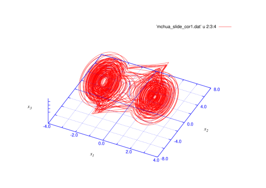
Figure 13: 3D phase portrait of the attractor shown in Figs. 12 for the same set of parameters.

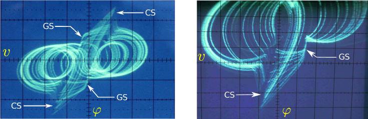
Figure 14: The phase portrait in the $(\phi-v_{1})$ plane for $L=26.76mH$, $C_{1}=40.77pF$, $C_{2}=98.79nF$, $R=740\Omega$, strength of the external forcing as $F_{o}=1.864KHz$ and frequency as $\Omega=1864Hz$. The arrows show clearly the crossing-sliding $CS$ and the grazing-sliding $GS$ interactions of the trajectories with the switching manifolds $\Sigma_{1,2}$ and $\Sigma_{2,3}$.

Similarly in Fig. 12(c), we find that the trajectories undergo grazing sliding interactions with the switching manifolds $\Sigma_{1,2}$ and $\Sigma_{2,3}$ at the points of crossings, shown by the arrows. The portrait in Fig. 12(d) show the enlargements of a portion of the phase portrait showing grazing sliding bifurcations with the switching manifold $\Sigma_{2,3}$. The 3D phase portrait of the attractor shown in Figs. 12 for the same set of parameters is shown in Fig. 13.

6.2 Experimental Verification

The crossing-sliding and grazing-sliding bifurcations are verified experimentally. For this the circuit parameters are chosen as $L=26.76$ mH, $C_{1}=40.77$ pF, $C_{2}=98.79$ nF, $R=740\Omega$, strength of the external forcing as $F_{o}=1.864$ KHz and frequency as $\Omega=1864$ Hz. The phase portrait obtained in the $(\phi-v_{1})$ plane is shown in Fig. 14(a) and a blown up portion of the same is shown in 14(b) for greater clarity.

7 Conclusion

In this paper, we have listed the different types of sliding bifurcations exhibited by a general n-dimensional non-smooth system and the conditions for the occurrence of the same. We have also given the analytic expressions for the zero-time discontinuity mapping corrections for realizing these numerically. Next we have described the piecewise-smooth characteristic of the active flux-controlled memristor in the $(\phi-q(\phi))$ and $(\phi-W(\phi))$ planes. Further we have obtained its $(v-i)$ characteristic using numerical simulations and hardware experiments. Though experimental studies for memristors have been reported previously, these are for memristors having smooth nonlinear characteristic. However we believe that it is for the first time that the experimental results of a memristor having nonlinear characteristic been reported.

We have then described the memristive MLC circuit and the memristive driven Chua oscillator constructed using this memristor, written their circuit equations and their normalized forms using proper rescaling parameters, converted them into Filippov systems by proper choice of parameters, identified the sliding bifurcations exhibited by each one of them, and derived the conditions as well as discontinuity corrections for observing them numerically. Further we have studied the sliding bifurcation induced dynamics and given experimental evidence for them.

Our studies have shown that the three segment piecewise-linear characteristic analog memristor model that we have designed earlier, is a robust one. This model can be used successfully to convert any standard nonlinear circuit into its memristive equivalent and then can be explored for its non-smooth dynamics. This may help in realizing the electric or electronic analogue of many of the mechanical systems whose non-smooth dynamics have been well investigated. Further studies to investigate the other types of discontinuity induced bifurcations such as stick-slip oscillations, impact oscillations, border-collision bifurcations and corner-collision bifurcations etc., in these circuits can be made. We have already initiated work on these lines and will be presenting them in future works.

Acknowledgments This work has been supported by DST-SERB Distinguished Fellowship Program (SB/DF/04/2017) of M.L. M.L acknowledges the financial support by DST-SERB Distinguished Fellowship Program (EMR/2014/001076), Government of India.

References

- Andronov et al. [2000] Andronov, A. A., Khaikin, S. E. & Vitt, A. A. [2000] Theory of Oscillations (Pergamon Press, Oxford).
- Anishchenko et al. [1993] Anishchenko, V. S., Safonova, M. & Chua, L. [1993] “Stochastic resonance in the nonautonomous Chua’s circuit,” J. Cir. Syst. Comput. 3, 553–578.
- Babitskii [1978] Babitskii, V. I. [1978] Theory of Vibroimpact Systems: Approximate Methods (Nauka, Moscow).
- Brogliato [1999] Brogliato, B. [1999] Nonsmooth Mechanics-Models, Dynamics and Control (Springer-Verlag, New York).
- Brogliato [2000] Brogliato, B. [2000] Impacts in Mechanical systems - Analysis and Modelling, in Lecture Notes in Physics, Vol. 551 (Springer-Verlag, New York).
- di Bernado et al. [2008] di Bernado, M., Budd, C., Champneys, A. & Kowalczyk, P. [2008] Piecewise-smooth Dynamical Systems: Theory and Applications (Springer-Verlag, London).
- di Bernado et al. [2001a] di Bernado, M., Budd, C. J. & Champneys, A. R. [2001a] “Normal form maps for grazing bifurcations in n-dimensional piecewise-smooth dynamical systems,” Physica D 160, 222–254.
- di Bernado et al. [1999] di Bernado, M., Feigin, M. I., Hogan, S. J. & Homer, M. E. [1999] “Local analysis of C-bifurcations in n-dimensional piecewise-smooth dynamical systems,” Chaos, Solitons and Fractals 10, 1881–1908.
- di Bernado et al. [2001b] di Bernado, M., Johansson, K. H. & Vasca, F. [2001b] “Self-oscillations and sliding in relay feedback systems: Symmetry and bifurcations,” Int. J. Bifurcation and Chaos. 11, 1121–1140.
- di Bernado et al. [2002] di Bernado, M., Kowalczyk, P. & Nordmark, A. [2002] “Bifurcations of dynamical systems with sliding: Derivation of normal-form mappings,” Physica D 170, 175–205.
- di Bernado et al. [2003] di Bernado, M., Kowalczyk, P. & Nordmark, A. [2003] “Sliding bifurcations: A novel mechanism for sudden onset of chaos in friction oscillators,” Int. J. Bifurcation and Chaos. 13, 2935–2948.
- di Bernardo et al. [2002] di Bernardo, M., Garofalo, F., Ianelli, L. & Vasca, F. [2002] “Bifurcations in piecewise-smooth feedback systems,” International Journal of Control. 75, 1243 –1259.
- Elwakil [2002] Elwakil, A. S. [2002] “Strange nonchaotic attractors of Chua’s circuit with quasiperiodic excitation,” Microelectronics J 33, 479–486.
- Feigin [1970] Feigin, M. [1970] “Doubling of the oscillation period with C-bifurcations in piecewise continuous systems,” Journal of Applied Mathematics and Mechanics 34, 861–869.
- Feigin [1994] Feigin, M. [1994] Forced Oscillations in Systems with Discontinuous Nonlinearities (Nauka, Moscow).
- Filippov [1964] Filippov, A. [1964] “Differential equations with discontinuous righthand-side,” American Mathematical Society Translations, Series 2 42, 199–231.
- Filippov [1988] Filippov, A. [1988] Differential Equations with Discontinuous Righthand Sides, Mathematics and its Applications (Kluwer Academic Publishers, Dortrecht).
- Ishaq & Lakshmanan [2013] Ishaq, A. A. & Lakshmanan, M. [2013] “Nonsmooth bifurcations, transient hyperchaos and hyperchaotic beats in a memristive Murali-Lakshmanan-Chua circuit,” Int. J. Bifurcation and Chaos 23, 1350098 (28 pages).
- Ishaq & Lakshmanan [2017] Ishaq, A. A. & Lakshmanan, M. [2017] “Discontinuity induced hopf and neimark-sacker bifurcations in a memristive Murali-Lakshmanan-Chua circuit,” Int. J. Bifurcation and Chaos 27, 1350098 (28 pages).
- Ishaq et al. [2011] Ishaq, A. A., Srinivasan, K., Murali, K. & Lakshmanan, M. [2011] “Observation of chaotic beats in a driven memristive Chua’s circuit,” Int. J. Bifurcation and Chaos. 21, 737–757.
- Itoh & Chua [2008] Itoh, M. & Chua, L. O. [2008] “Memristor oscillators,” Int. J. Bifurcation and Chaos. 18, 3183–3206.
- Kowalczyk & di Bernado [2001] Kowalczyk, P. & di Bernado, M. [2001] “On a novel class of bifurcations in hybrid dynamical systems - the case of relay feedback systems,” Proc. of Hybrid Systems Computation and Control (Springer-Verlag), pp. 361–374.
- Kunze [2000] Kunze, M. [2000] Non-smooth Dynamical Systems, in Lecture Notes in Mathematics, Vol. 1744 (Springer-Verlag, Berlin).
- Lakshmanan & Murali [1991] Lakshmanan, M. & Murali, K. [1991] “Bifurcation and chaos of the sinusoidally-driven Chua’s circuit,” Int. J. Bifurcation and Chaos. 1, 369–384.
- Leine & Campen [2002] Leine, R. I. & Campen, D. H. [2002] “Discontinuous fold bifurcations in mechanical systems,” Archive of Applied Mechanics 72, 138–146.
- Leine & Nijmeijer [2004] Leine, R. I. & Nijmeijer, H. [2004] Dynamics and Bifurcations in Non-smooth Mechanical Systems (Springer-Verlag, Berlin).
- Mosekilde & Zhusubalyev [2003] Mosekilde, E. & Zhusubalyev, Z. [2003] Bifurcations and Chaos in Piecewise-smooth Dynamical Systems (World Scientific, Singapore).
- Murali & Lakshmanan [1992a] Murali, K. & Lakshmanan [1992a] “Transition from quasiperiodicity to chaos and devil’s staircase structures of the driven Chua’s circuit,” Int. J. Bifurcation and Chaos. 2, 621–632.
- Murali & Lakshmanan [1990] Murali, K. & Lakshmanan, M. [1990] “Observation of many bifurcation sequences in a driven piecewise-linear circuit,” Phys. Lett A. 151, 412–419.
- Murali & Lakshmanan [1992b] Murali, K. & Lakshmanan, M. [1992b] “Chaotic dynamics of the driven Chua’s circuit,” IEEE Trans. Circuits and Syst.-1.: Fundamental Theory and Applications 40, 836–840.
- Murali & Lakshmanan [1992c] Murali, K. & Lakshmanan, M. [1992c] “Effect of sinusoidal excitation on the Chua’s circuit,” IEEE Trans. Circuits and Syst.-1.: Fundamental Theory and Applications 39, 264–270.
- Nordmark [1991] Nordmark, A. B. [1991] “Non-periodic motion caused by grazing incidence in impact oscillators,” Journal of Sound and Vibration 2, 279–297.
- Nusse & Yorke [1992] Nusse, H. E. & Yorke, J. A. [1992] “Border-collision bifurcations including period 2 to period 3 for piecewise smooth systems,” Physica D. 57, 39–57.
- Peterka [1974] Peterka, F. [1974] “Part 1:Theoretical analysis of n-multiple (1/n)-impact solutions,” CSAV Acta Technica 26, 462–473.
- Ronald [2014] Ronald, T. [2014] Memristors and Memristive Systems (Springer, New York).
- Srinivasan et al. [2009] Srinivasan, K., Thamilmaran, K. & Venkatesan, A. [2009] “Classification of bifurcation and chaos in Chua’s circuit with effect of different periodic forces,” Int. J. Bifurcation and Chaos. 19, 1951–1973.
- Utkin [1992] Utkin, V. [1992] Sliding Modes in Control Optimization (Springer-Verlag, Berlin).
- Zhu & Liu [1997] Zhu, Z. & Liu, Z. [1997] “Strange nonchaotic attractors of Chua’s circuit with quasiperiodic excitation,” Int. J. Bifurcation and Chaos. 7, 227–2256.