Equilibrium Propagation with
Continual Weight Updates

Maxence Ernoult1,2, Julie Grollier2, Damien Querlioz1, Yoshua Bengio3,4, Benjamin Scellier3
1
Centre de Nanosciences et de Nanotechnologies, Université Paris-Saclay
2Unité Mixte de Physique, CNRS, Thales, Université Paris-Saclay
3Mila, Université de Montréal
4Canadian Institute for Advanced Research
Abstract

Equilibrium Propagation (EP) is a learning algorithm that bridges Machine Learning and Neuroscience, by computing gradients closely matching those of Backpropagation Through Time (BPTT), but with a learning rule local in space. Given an input x𝑥x and associated target y𝑦y, EP proceeds in two phases: in the first phase neurons evolve freely towards a first steady state; in the second phase output neurons are nudged towards y𝑦y until they reach a second steady state. However, in existing implementations of EP, the learning rule is not local in time: the weight update is performed after the dynamics of the second phase have converged and requires information of the first phase that is no longer available physically. In this work, we propose a version of EP named Continual Equilibrium Propagation (C-EP) where neuron and synapse dynamics occur simultaneously throughout the second phase, so that the weight update becomes local in time. Such a learning rule local both in space and time opens the possibility of an extremely energy efficient hardware implementation of EP. We prove theoretically that, provided the learning rates are sufficiently small, at each time step of the second phase the dynamics of neurons and synapses follow the gradients of the loss given by BPTT (Theorem 1). We demonstrate training with C-EP on MNIST and generalize C-EP to neural networks where neurons are connected by asymmetric connections. We show through experiments that the more the network updates follows the gradients of BPTT, the best it performs in terms of training. These results bring EP a step closer to biology by better complying with hardware constraints while maintaining its intimate link with backpropagation.

1 Introduction

In the deep learning approach to AI (LeCun et al., 2015), backpropagation thrives as the most powerful algorithm for training artificial neural networks. It is interesting to note that its implementation on conventional computers or dedicated hardware consumes more energy than the brain by several orders of magnitude (Strubell et al., 2019). One path towards reducing the gap between brains and machines in terms of power consumption is by investigating alternative learning paradigms relying, as synapses do in the brain, on locally available information. Such local learning rules could be used for the development of extremely energy efficient learning-capable hardware, taking inspiration from information-encoding, dynamics and topology of the brain to achieve fast and energy efficient AI (Ambrogio et al., 2018; Romera et al., 2018).

In these regards, Equilibrium Propagation (EP) is an alternative style of computation for estimating error gradients that presents significant advantages (Scellier and Bengio, 2017). EP belongs to the family of contrastive Hebbian learning (CHL) algorithms (Ackley et al., 1985; Movellan, 1991; Hinton, 2002), in which neural dynamics and synaptic updates depend solely on information that is locally available. As a CHL algorithm, EP applies to convergent RNNs, which by definition are fed by a static input and converge to a steady state. Training such a network consists in adjusting the weights so that the steady state corresponding to an input x𝑥x produces output values close to associated targets y𝑦y. CHL algorithms proceed in two phases: first, conditioned on x𝑥x, neurons evolve freely without external influence and settle to a (first) steady state; second, the values of output neurons are pulled towards the target y𝑦y and the neurons settle to a second steady state. CHL weight updates consist in a Hebbian rule strengthening the connections between co-activated neurons at the first steady state, and an anti-Hebbian rule with opposite effects at the second steady state. A difference between Equilibrium Propagation and standard CHL algorithms is that output neurons are not clamped in the second phase but elastically pulled towards slightly reducing the loss value.

A second key property of EP is that, unlike CHL and related algorithms, it is intimately linked to backpropagation. It has been shown that synaptic updates in EP compute gradients of recurrent backpropagation (RBP) (Scellier and Bengio, 2019) and backpropagation through time (BPTT) (Ernoult et al., 2019). This makes EP especially attractive to bridge the gap between neural networks developed by neuroscientists, neuromorphic researchers and deep learning researchers.

Nevertheless, the bioplausibility of EP still undergoes two major limitations. First, although EP is local in space, it is non-local in time. In all existing implementations of EP the weight update is performed after the dynamics of the second phase have converged, when the first steady state is no longer physically available: the first steady state has to be stored. Second, the network dynamics have to derive from a primitive function which, in the Hopfield model, translates into to the requirement of symmetric weights. These two requirements are biologically unrealistic and also hinder the development of efficient EP computing hardware.

In this work, we propose an alternative implementation of EP, called Continual Equilibrium Propagation (C-EP) which features temporal locality, by enabling synaptic dynamics to occur throughout the second phase, simultaneously with neural dynamics. We then address the second issue by adapting C-EP to systems having asymmetric synaptic connections, taking inspiration from Scellier et al. (2018); we call this modified version the Continual Vector Field approach (or C-VF).

More specifically, the contributions of the current paper are the following:

  • We introduce C-EP (Section 3.1-3.2), a new version of EP with continual weight updates. Like standard EP, the C-EP algorithm applies to networks whose synaptic connections between neurons are assumed to be symmetric and tied.

  • We show mathematically that, provided that the changes in synaptic strengths are sufficiently slow (i.e. the learning rates are sufficiently small), at each time step of the second phase the dynamics of neurons and synapses follow the gradients of the loss obtained with BPTT (Theorem 1 and Fig. 2, Section 3.3). We call this property the Gradient Descending Dynamics (GDD) property, following the terminology used in Ernoult et al. (2019).

  • We demonstrate training with C-EP on MNIST, with accuracy approaching the one obtained with standard EP (Section 4.2).

  • We adapt C-EP to the more bio-realistic situation of a neural network with asymmetric connections between neurons. We call this C-VF as it is inspired by the Vector Field method proposed in Scellier et al. (2018). We demonstrate this approach on MNIST, and show numerically that the training performance is correlated with the satisfaction of the Gradient Descending Dynamics property (Section 4.3).

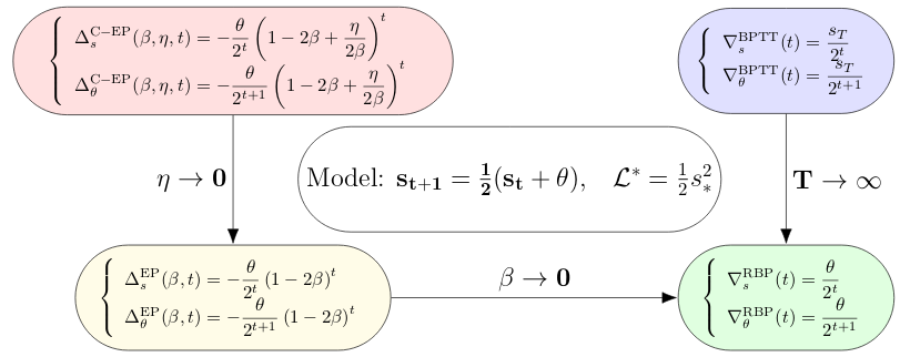
  • We also show how the Recurrent Backpropagation (RBP) algorithm of Almeida (1990); Pineda (1987b) relates to C-EP, EP and BPTT. We illustrate the equivalence of these four algorithms on a simple analytical model (Fig. 3) and we develop their general relationship in Appendix A.

2 Background: Convergent RNNs and Equilibrium Propagation

Convergent RNNs With Static Input.

We consider the supervised setting, where we want to predict a target y𝑦y given an input x𝑥x. The model is a recurrent neural network (RNN) parametrized by θ𝜃\theta and evolving according to the dynamics:

st+1=F(x,st,θ).subscript𝑠𝑡1𝐹𝑥subscript𝑠𝑡𝜃s_{t+1}=F\left(x,s_{t},\theta\right). (1)

F𝐹F is the transition function of the system. Assuming convergence of the dynamics before time step T𝑇T, we have sT=ssubscript𝑠𝑇subscript𝑠s_{T}=s_{*} where ssubscript𝑠s_{*} is the steady state of the network characterized by

s=F(x,s,θ).subscript𝑠𝐹𝑥subscript𝑠𝜃s_{*}=F\left(x,s_{*},\theta\right). (2)

The number of timesteps T𝑇T is a hyperparameter that we choose large enough so that sT=ssubscript𝑠𝑇subscript𝑠s_{T}=s_{*} for the current value of θ𝜃\theta. The goal is to optimize the parameter θ𝜃\theta in order to minimize a loss:

=(s,y).superscriptsubscript𝑠𝑦{\mathcal{L}^{*}}=\ell\left(s_{*},y\right). (3)

Algorithms that optimize the loss superscript{\mathcal{L}^{*}} for RNNs include Backpropagation Through Time (BPTT) and the Recurrent Backpropagation (RBP) algorithm of Almeida (1987); Pineda (1987a), presented in Appendix B.

Equilibrium Propagation (EP).

EP (Scellier and Bengio, 2017) is a learning algorithm that computes the gradient of superscript{\mathcal{L}}^{*} in the particular case where the transition function F derives from a scalar function ΦΦ\Phi, i.e. with F𝐹F of the form F(x,s,θ)=Φs(x,s,θ)𝐹𝑥𝑠𝜃Φ𝑠𝑥𝑠𝜃F(x,s,\theta)=\frac{\partial\Phi}{\partial s}(x,s,\theta). The algorithm consists in two phases (see Alg. 1 of Fig. 1). During the first phase, the network follows a sequence of states s1,s2,s3subscript𝑠1subscript𝑠2subscript𝑠3s_{1},s_{2},s_{3}\ldots and converges to a steady state denoted ssubscript𝑠s_{*}. In the second phase, an extra term βs𝛽𝑠\beta\;\frac{\partial\ell}{\partial s} pertubs the dynamics of the neurons (where β>0𝛽0\beta>0 is a scalar hyperparameter): starting from the steady state s0β=ssuperscriptsubscript𝑠0𝛽subscript𝑠s_{0}^{\beta}=s_{*}, the network follows a second sequence of states s1β,s2β,s3βsuperscriptsubscript𝑠1𝛽superscriptsubscript𝑠2𝛽superscriptsubscript𝑠3𝛽s_{1}^{\beta},s_{2}^{\beta},s_{3}^{\beta}\ldots and converges to a new steady state denoted sβsuperscriptsubscript𝑠𝛽s_{*}^{\beta}. Scellier and Bengio (2017) have shown that the gradient of the loss superscript{\mathcal{L}}^{*} can be estimated based on the two steady states ssubscript𝑠s_{*} and sβsuperscriptsubscript𝑠𝛽s_{*}^{\beta}. Specifically, in the limit β0𝛽0\beta\to 0,

1β(Φθ(x,sβ,θ)Φθ(x,s,θ))θ.1𝛽Φ𝜃𝑥superscriptsubscript𝑠𝛽𝜃Φ𝜃𝑥subscript𝑠𝜃superscript𝜃\frac{1}{\beta}\left(\frac{\partial\Phi}{\partial\theta}\left(x,s_{*}^{\beta},\theta\right)-\frac{\partial\Phi}{\partial\theta}\left(x,s_{*},\theta\right)\right)\to-\frac{\partial{\mathcal{L}}^{*}}{\partial\theta}. (4)

3 Equilibrium Propagation with Continual Weight Updates (C-EP)

This section presents the main theoretical contributions of this paper. We introduce a new algorithm to optimize superscript{\mathcal{L}^{*}} (Eq. 3): a new version of EP with continual parameter updates that we call C-EP. Unlike typical machine learning algorithms (such as BPTT, RBP and EP) in which the weight updates occur after all the other computations in the system are performed, our algorithm offers a mechanism in which the weights are updated continuously as the states of the neurons change.

Input: x𝑥x, y𝑦y, θ𝜃\theta, β𝛽\beta, η𝜂\eta.
Output: θ𝜃\theta.

Algorithm 1 EP
1:s00subscript𝑠00s_{0}\leftarrow 0 \triangleright First Phase
2:repeat
3:     st+1Φs(x,st,θ)subscript𝑠𝑡1Φ𝑠𝑥subscript𝑠𝑡𝜃s_{t+1}\leftarrow\frac{\partial\Phi}{\partial s}\left(x,s_{t},\theta\right)
4:until st=ssubscript𝑠𝑡subscript𝑠s_{t}=s_{*}
5:Store ssubscript𝑠s_{*}
6:s0βssuperscriptsubscript𝑠0𝛽subscript𝑠s_{0}^{\beta}\leftarrow s_{*} \triangleright Second Phase
7:repeat
8:     st+1βΦs(x,stβ,θ)βs(stβ,y)superscriptsubscript𝑠𝑡1𝛽Φ𝑠𝑥superscriptsubscript𝑠𝑡𝛽𝜃𝛽𝑠superscriptsubscript𝑠𝑡𝛽𝑦s_{t+1}^{\beta}\leftarrow\frac{\partial\Phi}{\partial s}\left(x,s_{t}^{\beta},\theta\right)-\beta\frac{\partial\ell}{\partial s}\left(s_{t}^{\beta},y\right)
9:until stβ=sβsuperscriptsubscript𝑠𝑡𝛽superscriptsubscript𝑠𝛽s_{t}^{\beta}=s_{*}^{\beta}
10:\triangleright Global Parameter Update
11:θθ+ηβ(Φθ(sβ,θ)Φθ(s,θ))𝜃𝜃𝜂𝛽Φ𝜃superscriptsubscript𝑠𝛽𝜃Φ𝜃subscript𝑠𝜃\theta\leftarrow\theta+\frac{\eta}{\beta}\left(\frac{\partial\Phi}{\partial\theta}\left(s_{*}^{\beta},\theta\right)-\frac{\partial\Phi}{\partial\theta}\left(s_{*},\theta\right)\right)

Input: x𝑥x, y𝑦y, θ𝜃\theta, β𝛽\beta, η𝜂\eta.
Output: θ𝜃\theta.

Algorithm 2 C-EP (with simplified notations)
1:s00subscript𝑠00s_{0}\leftarrow 0 \triangleright First Phase
2:repeat
3:     st+1Φs(x,st,θ)subscript𝑠𝑡1Φ𝑠𝑥subscript𝑠𝑡𝜃s_{t+1}\leftarrow\frac{\partial\Phi}{\partial s}\left(x,s_{t},\theta\right)
4:until st=ssubscript𝑠𝑡subscript𝑠s_{t}=s_{*}
5:s0βssuperscriptsubscript𝑠0𝛽subscript𝑠s_{0}^{\beta}\leftarrow s_{*} \triangleright Second Phase
6:repeat
7:     st+1βΦs(x,stβ,θ)βs(stβ,y)superscriptsubscript𝑠𝑡1𝛽Φ𝑠𝑥superscriptsubscript𝑠𝑡𝛽𝜃𝛽𝑠superscriptsubscript𝑠𝑡𝛽𝑦s_{t+1}^{\beta}\leftarrow\frac{\partial\Phi}{\partial s}\left(x,s_{t}^{\beta},\theta\right)-\beta\frac{\partial\ell}{\partial s}\left(s_{t}^{\beta},y\right)
8:     \triangleright Parameter Update at Time t𝑡t
9:     θθ+ηβ(Φθ(st+1β)Φθ(stβ))𝜃𝜃𝜂𝛽Φ𝜃superscriptsubscript𝑠𝑡1𝛽Φ𝜃superscriptsubscript𝑠𝑡𝛽\theta\leftarrow\theta+\frac{\eta}{\beta}\left(\frac{\partial\Phi}{\partial\theta}\left(s_{t+1}^{\beta}\right)-\frac{\partial\Phi}{\partial\theta}\left(s_{t}^{\beta}\right)\right)
10:until stβsuperscriptsubscript𝑠𝑡𝛽s_{t}^{\beta} and θ𝜃\theta are converged.
Figure 1: Left. Pseudo-code of EP. This is the version of EP for discrete-time dynamics introduced in Ernoult et al. (2019). Right. Pseudo-code of C-EP with simplified notations (see section 3.2 for a formal definition of C-EP). Difference between EP and C-EP. In EP, one global parameter update is performed at the end of the second phase ; in C-EP, parameter updates are performed throughout the second phase. Eq. 5 shows that the continual updates of C-EP add up to the global update of EP.

3.1 From EP to C-EP: An intuition behind continual weight updates

The key idea to understand how to go from EP to C-EP is that the gradient of EP appearing in Eq. (4) reads as the following telescopic sum:

1β(Φθ(x,sβ,θ)Φθ(x,s,θ))global parameter gradient in EP=t=11β(Φθ(x,stβ,θ)Φθ(x,st1β,θ))parameter gradient at time t in C-EP.subscript1𝛽Φ𝜃𝑥superscriptsubscript𝑠𝛽𝜃Φ𝜃𝑥subscript𝑠𝜃global parameter gradient in EPsuperscriptsubscript𝑡1subscript1𝛽Φ𝜃𝑥superscriptsubscript𝑠𝑡𝛽𝜃Φ𝜃𝑥superscriptsubscript𝑠𝑡1𝛽𝜃parameter gradient at time t in C-EP\underbrace{\frac{1}{\beta}\left(\frac{\partial\Phi}{\partial\theta}\left(x,s_{*}^{\beta},\theta\right)-\frac{\partial\Phi}{\partial\theta}\left(x,s_{*},\theta\right)\right)}_{\text{global parameter gradient in EP}}=\sum_{t=1}^{\infty}\underbrace{\frac{1}{\beta}\left(\frac{\partial\Phi}{\partial\theta}\left(x,s_{t}^{\beta},\theta\right)-\frac{\partial\Phi}{\partial\theta}\left(x,s_{t-1}^{\beta},\theta\right)\right)}_{\text{parameter gradient at time t in C-EP}}. (5)

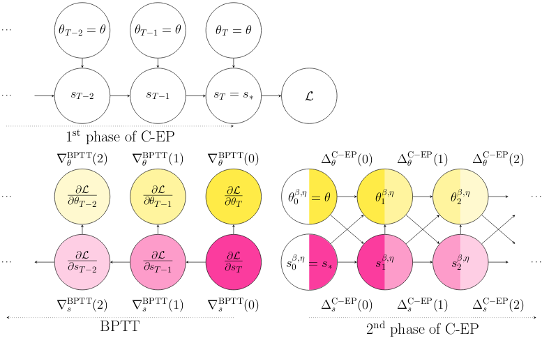
In Eq. (5) we have used that s0β=ssuperscriptsubscript𝑠0𝛽subscript𝑠s_{0}^{\beta}=s_{*} and stβsβsuperscriptsubscript𝑠𝑡𝛽superscriptsubscript𝑠𝛽s_{t}^{\beta}\to s_{*}^{\beta} as t𝑡t\to\infty. Here lies the very intuition of continual updates motivating this work; instead of keeping the weights fixed throughout the second phase and updating them at the end of the second phase based on the steady states ssubscript𝑠s_{*} and sβsuperscriptsubscript𝑠𝛽s_{*}^{\beta}, as in EP (Alg. 1 of Fig. 1), the idea of the C-EP algorithm is to update the weights at each time t𝑡t of the second phase between two consecutive states st1βsuperscriptsubscript𝑠𝑡1𝛽s_{t-1}^{\beta} and stβsuperscriptsubscript𝑠𝑡𝛽s_{t}^{\beta} (Alg. 2 of Fig. 1). One key difference in C-EP compared to EP though, is that, in the second phase, the weight update at time step t𝑡t influences the neural states at time step t+1𝑡1t+1 in a nontrivial way, as illustrated in the computational graph of Fig. 2. In the next subsection we define C-EP using notations that explicitly show this dependency.

3.2 Description of the C-EP algorithm

The first phase of C-EP is the same as that of EP (see Fig. 1). In the second phase of C-EP the parameter variable is regarded as another dynamic variable θtsubscript𝜃𝑡\theta_{t} that evolves with time t𝑡t along with stsubscript𝑠𝑡s_{t}. The dynamics of stsubscript𝑠𝑡s_{t} and θtsubscript𝜃𝑡\theta_{t} in the second phase of C-EP depend on the values of the two hyperparameters β𝛽\beta (the hyperparameter of influence) and η𝜂\eta (the learning rate), therefore we write stβ,ηsuperscriptsubscript𝑠𝑡𝛽𝜂s_{t}^{\beta,\eta} and θtβ,ηsuperscriptsubscript𝜃𝑡𝛽𝜂\theta_{t}^{\beta,\eta} to show explicitly this dependence. With now both the neurons and the synapses evolving in the second phase, the dynamic variables stβ,ηsuperscriptsubscript𝑠𝑡𝛽𝜂s_{t}^{\beta,\eta} and θtβ,ηsuperscriptsubscript𝜃𝑡𝛽𝜂\theta_{t}^{\beta,\eta} start from s0β,η=ssuperscriptsubscript𝑠0𝛽𝜂subscript𝑠s_{0}^{\beta,\eta}=s_{*} and θ0β,η=θsuperscriptsubscript𝜃0𝛽𝜂𝜃\theta_{0}^{\beta,\eta}=\theta and follow:

t0:{st+1β,η=Φs(x,stβ,η,θtβ,η)βs(stβ,η,y),θt+1β,η=θtβ,η+ηβ(Φθ(x,st+1β,η,θtβ,η)Φθ(x,stβ,η,θtβ,η)).\displaystyle\forall t\geq 0:\qquad\left\{\begin{array}[]{l}\displaystyle s_{t+1}^{\beta,\eta}=\frac{\partial\Phi}{\partial s}\left(x,s_{t}^{\beta,\eta},\theta_{t}^{\beta,\eta}\right)-\beta\;\frac{\partial\ell}{\partial s}\left(s_{t}^{\beta,\eta},y\right),\\ \displaystyle\theta_{t+1}^{\beta,\eta}=\theta_{t}^{\beta,\eta}+\frac{\eta}{\beta}\left(\frac{\partial\Phi}{\partial\theta}\left(x,s_{t+1}^{\beta,\eta},\theta_{t}^{\beta,\eta}\right)-\frac{\partial\Phi}{\partial\theta}\left(x,s_{t}^{\beta,\eta},\theta_{t}^{\beta,\eta}\right)\right).\end{array}\right. (8)

The difference in C-EP compared to EP is that the value of the parameter used to update st+1β,ηsuperscriptsubscript𝑠𝑡1𝛽𝜂s_{t+1}^{\beta,\eta} in Eq. (8) is the current θtβ,ηsuperscriptsubscript𝜃𝑡𝛽𝜂\theta_{t}^{\beta,\eta}, not θ𝜃\theta. Provided the learning rate η𝜂\eta is small enough, i.e. the synapses are slow compared to the neurons, this effect is weak. Intuitively, in the limit η0𝜂0\eta\to 0, the parameter changes are negligible so that θtβ,ηsuperscriptsubscript𝜃𝑡𝛽𝜂\theta_{t}^{\beta,\eta} can be approximated by its initial value θ0β,η=θsuperscriptsubscript𝜃0𝛽𝜂𝜃\theta_{0}^{\beta,\eta}=\theta. Under this approximation, the dynamics of stβ,ηsuperscriptsubscript𝑠𝑡𝛽𝜂s_{t}^{\beta,\eta} in C-EP and the dynamics of stβsuperscriptsubscript𝑠𝑡𝛽s_{t}^{\beta} in EP are the same. See Fig. 3 for a simple example, and Appendix A.3 for a proof in the general case.
Refer to caption

Figure 2: Gradient-Descending Dynamics (GDD, Theorem 1). In the second phase of Continual Equilibrium Prop (C-EP), the dynamics of neurons and synapses descend the gradients of BPTT, i.e. ΔCEP(t)=BPTT(t)superscriptΔCEP𝑡superscriptBPTT𝑡\Delta^{\rm C-EP}(t)=-\nabla^{\rm BPTT}(t). The colors illustrate when corresponding computations are realized in C-EP and BPTT. Top left. 1st phase of C-EP with static input x𝑥x and target y𝑦y. The final state sTsubscript𝑠𝑇s_{T} is the steady state ssubscript𝑠s_{*}. Bottom left. Backprop through time (BPTT). Bottom right. 2nd phase of C-EP. The starting state s0β,ηsuperscriptsubscript𝑠0𝛽𝜂s_{0}^{\beta,\eta} is the final state of the forward-time pass, i.e. the steady state ssubscript𝑠s_{*}.

3.3 Gradient-Descending Dynamics (GDD)

Now we prove that, provided the hyperparameter β𝛽\beta and the learning rate η𝜂\eta are small enough, the dynamics of the neurons and the weights given by Eq. (8) follow the gradients of BPTT (Theorem 1 and Fig. 2). For a formal statement of this property, we define the normalized (continual) updates of C-EP, as well as the gradients of the loss =(sT,y)subscript𝑠𝑇𝑦{\mathcal{L}}=\ell\left(s_{T},y\right) after T𝑇T time steps, computed with BPTT:

{ΔsCEP(β,η,t)=1β(st+1β,ηstβ,η),ΔθCEP(β,η,t)=1η(θt+1β,ηθtβ,η),{sBPTT(t)=sTt,θBPTT(t)=θTt.casessuperscriptsubscriptΔ𝑠CEP𝛽𝜂𝑡1𝛽superscriptsubscript𝑠𝑡1𝛽𝜂superscriptsubscript𝑠𝑡𝛽𝜂superscriptsubscriptΔ𝜃CEP𝛽𝜂𝑡1𝜂superscriptsubscript𝜃𝑡1𝛽𝜂superscriptsubscript𝜃𝑡𝛽𝜂casessubscriptsuperscriptBPTT𝑠𝑡subscript𝑠𝑇𝑡subscriptsuperscriptBPTT𝜃𝑡subscript𝜃𝑇𝑡\left\{\begin{array}[]{l}\displaystyle\Delta_{s}^{\rm C-EP}(\beta,\eta,t)=\frac{1}{\beta}\left(s_{t+1}^{\beta,\eta}-s_{t}^{\beta,\eta}\right),\\ \displaystyle\Delta_{\theta}^{\rm C-EP}(\beta,\eta,t)=\frac{1}{\eta}\left(\theta_{t+1}^{\beta,\eta}-\theta_{t}^{\beta,\eta}\right),\end{array}\right.\qquad\left\{\begin{array}[]{l}\displaystyle\nabla^{\rm BPTT}_{s}(t)=\frac{\partial{\mathcal{L}}}{\partial s_{T-t}},\\ \displaystyle\nabla^{\rm BPTT}_{\theta}(t)=\frac{\partial{\mathcal{L}}}{\partial\theta_{T-t}}.\end{array}\right. (9)

More details about {\mathcal{L}} and the gradients sBPTT(t)subscriptsuperscriptBPTT𝑠𝑡\nabla^{\rm BPTT}_{s}(t) and θBPTT(t)subscriptsuperscriptBPTT𝜃𝑡\nabla^{\rm BPTT}_{\theta}(t) are provided in Appendix B. Note that injecting Eq. (8) in Eq. (9), the normalized updates of C-EP consequently read:

ΔθCEP(β,η,t)=1β(Φθ(x,st+1β,η,θtβ,η)Φθ(x,stβ,η,θtβ,η)),superscriptsubscriptΔ𝜃CEP𝛽𝜂𝑡1𝛽Φ𝜃𝑥superscriptsubscript𝑠𝑡1𝛽𝜂superscriptsubscript𝜃𝑡𝛽𝜂Φ𝜃𝑥superscriptsubscript𝑠𝑡𝛽𝜂superscriptsubscript𝜃𝑡𝛽𝜂\Delta_{\theta}^{\rm C-EP}(\beta,\eta,t)=\frac{1}{\beta}\left(\frac{\partial\Phi}{\partial\theta}\left(x,s_{t+1}^{\beta,\eta},\theta_{t}^{\beta,\eta}\right)-\frac{\partial\Phi}{\partial\theta}\left(x,s_{t}^{\beta,\eta},\theta_{t}^{\beta,\eta}\right)\right), (10)

which corresponds to the parameter gradient at time t𝑡t, defined informally in Eq. (5). The following result makes this statement more formal.

Theorem 1 (GDD Property).

Let s0,s1,,sTsubscript𝑠0subscript𝑠1subscript𝑠𝑇s_{0},s_{1},\ldots,s_{T} be the convergent sequence of states and denote s=sTsubscript𝑠subscript𝑠𝑇s_{*}=s_{T} the steady state. Further assume that there exists some step K𝐾K where 0<KT0𝐾𝑇0<K\leq T such that s=sT=sT1=sTKsubscript𝑠subscript𝑠𝑇subscript𝑠𝑇1subscript𝑠𝑇𝐾s_{*}=s_{T}=s_{T-1}=\ldots s_{T-K}. Then, in the limit η0𝜂0\eta\to 0 and β0𝛽0\beta\to 0, the first K𝐾K normalized updates in the second phase of C-EP are equal to the negatives of the first K𝐾K gradients of BPTT, i.e.

t=0,1,,K:{limβ0limη0ΔsCEP(β,η,t)=sBPTT(t),limβ0limη0ΔθCEP(β,η,t)=θBPTT(t).\forall t=0,1,\ldots,K:\quad\left\{\begin{array}[]{ll}\displaystyle\lim_{\beta\to 0}\;\lim_{\eta\to 0}\;\Delta^{\rm C-EP}_{s}(\beta,\eta,t)=-\nabla^{\rm BPTT}_{s}(t),\\ \displaystyle\lim_{\beta\to 0}\;\lim_{\eta\to 0}\;\Delta^{\rm C-EP}_{\theta}(\beta,\eta,t)=-\nabla^{\rm BPTT}_{\theta}(t).\end{array}\right. (11)

Note the following two remarks:

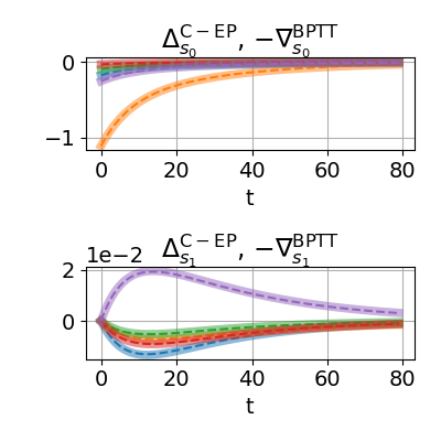
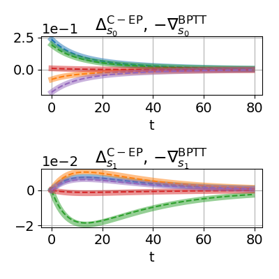
  • Fig. 3 illustrates Theorem 1 with a simple dynamical system for which the normalized updates ΔCEPsuperscriptΔCEP\Delta^{\rm C-EP} and the gradients BPTTsuperscriptBPTT\nabla^{\rm BPTT} are analytically tractable.

  • Theorem 1 rewrites st+1β,ηstβ,ηβsTtsuperscriptsubscript𝑠𝑡1𝛽𝜂superscriptsubscript𝑠𝑡𝛽𝜂𝛽subscript𝑠𝑇𝑡s_{t+1}^{\beta,\eta}\approx s_{t}^{\beta,\eta}-\beta\frac{\partial{\mathcal{L}}}{\partial s_{T-t}} and θt+1β,ηθtβ,ηηθTtsuperscriptsubscript𝜃𝑡1𝛽𝜂superscriptsubscript𝜃𝑡𝛽𝜂𝜂subscript𝜃𝑇𝑡\theta_{t+1}^{\beta,\eta}\approx\theta_{t}^{\beta,\eta}-\eta\frac{\partial{\mathcal{L}}}{\partial\theta_{T-t}}, showing that in the second phase of C-EP, neurons and synapses descend the gradients of the loss {\mathcal{L}} obtained with BPTT, with the hyperparameters β𝛽\beta and η𝜂\eta playing the role of learning rates for stβ,ηsuperscriptsubscript𝑠𝑡𝛽𝜂s_{t}^{\beta,\eta} and θtβ,ηsuperscriptsubscript𝜃𝑡𝛽𝜂\theta_{t}^{\beta,\eta}, respectively. Theorem 1 holds in the limit β0𝛽0\beta\to 0, η0𝜂0\eta\to 0, which means that β𝛽\beta and η𝜂\eta have to be small enough for the neurons and synapses to compute approximately the gradient of superscript{\mathcal{L}}^{*}. On the other hand β𝛽\beta and η𝜂\eta also have to be large enough so that an error signal can be transmitted in the second phase and that optimization of the loss happens within a reasonable number of epochs. This trade-off is well reflected by the table of hyperparameters of Table 2 in Appendix F.1. In particular, the values β=0𝛽0\beta=0 (there is no second phase) and (or) η=0𝜂0\eta=0 (there is no learning) are excluded.

Refer to caption

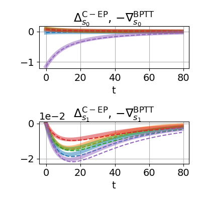
Figure 3: Illustration of Theorem 1 on a simple model. The variables s𝑠s and θ𝜃\theta are scalars, the first phase equation is st+1=12(st+θ)subscript𝑠𝑡112subscript𝑠𝑡𝜃s_{t+1}=\frac{1}{2}(s_{t}+\theta), the steady state is denoted ssubscript𝑠s_{*} and the loss is =12s2superscript12superscriptsubscript𝑠2{\mathcal{L}}^{*}=\frac{1}{2}s_{*}^{2}. For completeness, we also include the corresponding gradients of Recurrent Backpropagation (RBP) and the normalized updates of EP, denoted RBPsuperscriptRBP\nabla^{\rm RBP} and ΔEPsuperscriptΔEP\Delta^{\rm EP} respectively. The equivalence between C-EP, EP, RBP and BPTT holds in the general setting: see Appendix A for a thorough study of their relationship.

4 Numerical Experiments

In this section, we validate our continual version of Equilibrium Propagation against training on the MNIST data set with two models. The first model is a vanilla RNN with tied and symmetric weights: the dynamics of this model approximately derive from a primitive function, which allows training with C-EP. The second model is a Discrete-Time RNN with untied and asymmetric weights, which is therefore closer to biology. We train this second model with a modified version of C-EP which we call C-VF (Continual Vector Field) as it is inspired from the algorithm with Vector-Field dynamics of Scellier et al. (2018). Ernoult et al. (2019) showed with simulations the intuitive result that, if a model is such that the normalized updates of EP ‘match’ the gradients of BPTT (i.e. if they are approximately equal), then the model trained with EP performs as well as the model trained with BPTT. Along the same lines, we show in this work that the more the EP normalized updates follow the gradients of BPTT before training, the best is the resulting training performance. We choose to implement C-EP and C-VF on vanilla RNNs to accelerate simulations (Ernoult et al., 2019).

4.1 Models: Vanilla RNNs with symmetric and asymmetric weights

Vanilla RNN with symmetric weights trained by C-EP.

The first phase dynamics is defined as:

st+1=σ(Wst+Wxx),subscript𝑠𝑡1𝜎𝑊subscript𝑠𝑡subscript𝑊𝑥𝑥s_{t+1}=\sigma\left(W\cdot s_{t}+W_{x}\cdot x\right), (12)

where σ𝜎\sigma is an activation function, W𝑊W is a symmetric weight matrix, and Wxsubscript𝑊𝑥W_{x} is a matrix connecting x𝑥x to s𝑠s. Although the dynamics are not directly defined in terms of a primitive function, note that st+1Φs(st,W)subscript𝑠𝑡1Φ𝑠subscript𝑠𝑡𝑊s_{t+1}\approx\frac{\partial\Phi}{\partial s}\left(s_{t},W\right) with Φ(s,W)=12sWsΦ𝑠𝑊12superscript𝑠top𝑊𝑠\Phi(s,W)=\frac{1}{2}s^{\top}\cdot W\cdot s if we ignore the activation function σ𝜎\sigma. Following Eq. (8) and Eq. (9), we define the normalized updates of this model as:

ΔsCEP(β,η,t)superscriptsubscriptΔ𝑠CEP𝛽𝜂𝑡\displaystyle\Delta_{s}^{\rm C-EP}(\beta,\eta,t) =1β(st+1β,ηstβ,η),ΔWCEP(β,η,t)=1β(st+1β,ηst+1β,ηstβ,ηstβ,η),formulae-sequenceabsent1𝛽superscriptsubscript𝑠𝑡1𝛽𝜂superscriptsubscript𝑠𝑡𝛽𝜂superscriptsubscriptΔ𝑊CEP𝛽𝜂𝑡1𝛽superscriptsubscript𝑠𝑡1𝛽superscript𝜂topsuperscriptsubscript𝑠𝑡1𝛽𝜂superscriptsubscript𝑠𝑡𝛽superscript𝜂topsuperscriptsubscript𝑠𝑡𝛽𝜂\displaystyle=\frac{1}{\beta}\left(s_{t+1}^{\beta,\eta}-s_{t}^{\beta,\eta}\right),\quad\Delta_{W}^{\rm C-EP}(\beta,\eta,t)=\frac{1}{\beta}\left(s_{t+1}^{{\beta,\eta}^{\top}}\cdot s_{t+1}^{\beta,\eta}-s_{t}^{{\beta,\eta}^{\top}}\cdot s_{t}^{\beta,\eta}\right),
ΔWxCEP(β,η,t)superscriptsubscriptΔsubscript𝑊𝑥CEP𝛽𝜂𝑡\displaystyle\Delta_{W_{x}}^{\rm C-EP}(\beta,\eta,t) =1βx(st+1β,ηstβ,η).absent1𝛽superscript𝑥topsuperscriptsubscript𝑠𝑡1𝛽𝜂superscriptsubscript𝑠𝑡𝛽𝜂\displaystyle=\frac{1}{\beta}x^{\top}\cdot\left(s_{t+1}^{\beta,\eta}-s_{t}^{\beta,\eta}\right). (13)

Note that this model applies to any topology as long as existing connections have symmetric values: this includes deep networks with any number of layers – see Appendix E for detailed descriptions of the models used in the experiments. More explicitly, for a network whose layers of neurons are s0superscript𝑠0s^{0}, s1superscript𝑠1s^{1}, …, sNsuperscript𝑠𝑁s^{N}, with Wn,n+1subscript𝑊𝑛𝑛1W_{n,n+1} connecting the layers sn+1superscript𝑠𝑛1s^{n+1} and snsuperscript𝑠𝑛s^{n} in both directions, the corresponding primitive function is Φ=n(sn)Wn,n+1sn+1+sNWxxΦsubscript𝑛superscriptsuperscript𝑠𝑛topsubscript𝑊𝑛𝑛1subscript𝑠𝑛1superscript𝑠superscript𝑁topsubscript𝑊𝑥𝑥\Phi=\sum_{n}(s^{n})^{\top}\cdot W_{n,n+1}\cdot s_{n+1}+s^{N^{\top}}\cdot W_{x}\cdot x - see Appendix E.1 for more details.

Vanilla RNN with asymmetric weights trained by C-VF.

In this model, the dynamics in the first phase is the same as Eq. (12) but now the weight matrix W𝑊W is no longer assumed to be symmetric, i.e. the reciprocal connections between neurons are not constrained. In this setting the weight dynamics in the second phase is replaced by a version for asymmetric weights: Wt+1β,η=Wtβ,η+ηβstβ,η(st+1β,ηstβ,η)subscriptsuperscript𝑊𝛽𝜂𝑡1subscriptsuperscript𝑊𝛽𝜂𝑡𝜂𝛽superscriptsubscript𝑠𝑡𝛽superscript𝜂topsuperscriptsubscript𝑠𝑡1𝛽𝜂superscriptsubscript𝑠𝑡𝛽𝜂W^{\beta,\eta}_{t+1}=W^{\beta,\eta}_{t}+\frac{\eta}{\beta}s_{t}^{{\beta,\eta}^{\top}}\cdot\left(s_{t+1}^{\beta,\eta}-s_{t}^{\beta,\eta}\right), so that the normalized updates are equal to:

ΔsCVF(β,η,t)superscriptsubscriptΔ𝑠CVF𝛽𝜂𝑡\displaystyle\Delta_{s}^{\rm C-VF}(\beta,\eta,t) =1β(st+1β,ηstβ,η),ΔWCVF(β,η,t)=1βstβ,η(st+1β,ηstβ,η),formulae-sequenceabsent1𝛽superscriptsubscript𝑠𝑡1𝛽𝜂superscriptsubscript𝑠𝑡𝛽𝜂superscriptsubscriptΔ𝑊CVF𝛽𝜂𝑡1𝛽superscriptsubscript𝑠𝑡𝛽superscript𝜂topsuperscriptsubscript𝑠𝑡1𝛽𝜂superscriptsubscript𝑠𝑡𝛽𝜂\displaystyle=\frac{1}{\beta}\left(s_{t+1}^{\beta,\eta}-s_{t}^{\beta,\eta}\right),\qquad\Delta_{W}^{\rm C-VF}(\beta,\eta,t)=\frac{1}{\beta}s_{t}^{{\beta,\eta}^{\top}}\cdot\left(s_{t+1}^{\beta,\eta}-s_{t}^{\beta,\eta}\right),
ΔWxCVF(β,η,t)superscriptsubscriptΔsubscript𝑊𝑥CVF𝛽𝜂𝑡\displaystyle\Delta_{W_{x}}^{\rm C-VF}(\beta,\eta,t) =1βx(st+1β,ηstβ,η).absent1𝛽superscript𝑥topsuperscriptsubscript𝑠𝑡1𝛽𝜂superscriptsubscript𝑠𝑡𝛽𝜂\displaystyle=\frac{1}{\beta}x^{\top}\cdot\left(s_{t+1}^{\beta,\eta}-s_{t}^{\beta,\eta}\right). (14)

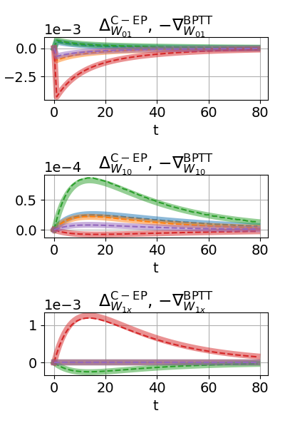
Like the previous model, the vanilla RNN with asymmetric weights also applies to deep networks with any number of layers. Although in C-VF the dynamics of the weights is not one of the form of Eq. (8) that derives from a primitive function, the (bioplausible) normalized weight updates of Eq. (14) can approximately follow the gradients of BPTT, provided that the values of reciprocal connections are not too dissimilar: this is illustrated in Fig. 5 (as well as in Fig. 12 and Fig. 13 of Appendix E.6) and proved in Appendix D.2. This property motivates the following training experiments.

Error (%percent\%) T K Epochs
Test Train
EP-1h 2.00±0.13plus-or-minus2.000.132.00\pm 0.13 (0.20)0.20(0.20) 30 10 30
EP-2h 1.95±0.10plus-or-minus1.950.101.95\pm 0.10 (0.14)0.14(0.14) 100 20 50
C-EP-1h 2.28±0.16plus-or-minus2.280.16\mathbf{2.28\pm 0.16} (0.41)0.41(0.41) 40 15 100
C-EP-2h 2.44±0.14plus-or-minus2.440.14\mathbf{2.44\pm 0.14} (0.31)0.31(0.31) 100 20 150
C-VF-1h 2.43±0.08plus-or-minus2.430.08\mathbf{2.43\pm 0.08} (0.77)0.77(0.77) 40 15 100
C-VF-2h 2.97±0.19plus-or-minus2.970.19\mathbf{2.97\pm 0.19} (1.58)1.58(1.58) 100 20 150
Refer to caption
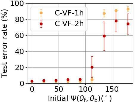
Figure 4: Left: Training results on MNIST with EP, C-EP and C-VF. "##\#h" stands for the number of hidden layers. We indicate over 5 trials the mean and standard deviation for the test error (mean train error in parenthesis). T𝑇T (resp. K𝐾K) is the number of iterations in the 1st (resp. 2nd) phase. For C-VF results, the initial angle between forward (θfsubscript𝜃f\theta_{\rm f}) and backward (θbsubscript𝜃b\theta_{\rm b}) weights is Ψ(θf,θb)=0Ψsubscript𝜃fsubscript𝜃bsuperscript0\Psi(\theta_{\rm f},\theta_{\rm b})=0^{\circ}. Right: Test error rate on MNIST achieved by C-VF as a function of the initial Ψ(θf,θb)Ψsubscript𝜃fsubscript𝜃b\Psi(\theta_{\rm f},\theta_{\rm b}).

4.2 C-EP training experiments

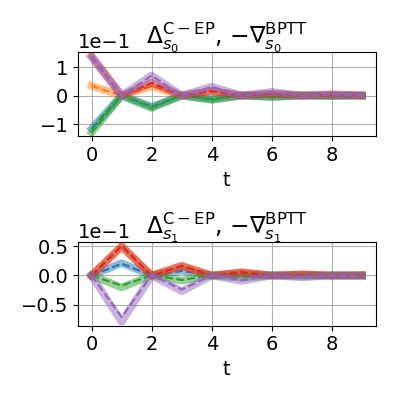
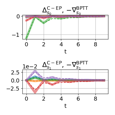
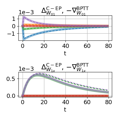
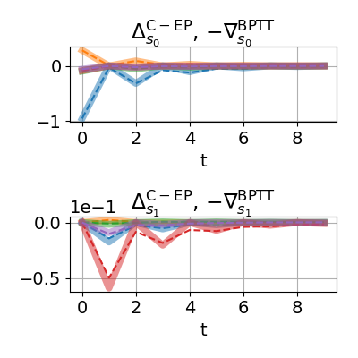
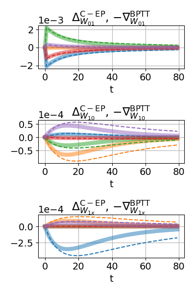
Experiments are performed with multi-layered vanilla RNNs (with symmetric weights) on MNIST. The table of Fig. 4 presents the results obtained with C-EP training benchmarked against standard EP training (Ernoult et al., 2019) - see Appendix E for model details and Appendix F.1 for training conditions. Although the test error of C-EP approaches that of EP, we observe a degradation in accuracy. This is because although Theorem 1 guarantees Gradient Descending Dynamics (GDD) in the limit of infinitely small learning rates, in practice we have to strike a balance between having a learning rate that is small enough to ensure this condition but not too small to observe convergence within a reasonable number of epochs. As seen on Fig. 5 (b), the finite learning rate η𝜂\eta of continual updates leads to ΔCEP(β,η,t)superscriptΔCEP𝛽𝜂𝑡\Delta^{\rm C-EP}(\beta,\eta,t) curves splitting apart from the BPTT(t)superscriptBPTT𝑡-\nabla^{\rm BPTT}(t) curves. As seen per Fig. 5 (a), this effect is emphasized with the depth: before training, angles between the normalized updates of C-EP and the gradients of BPTT reach 50 degrees for two hidden layers. The deeper the network, the more difficult it is for the C-EP dynamics to follow the gradients provided by BPTT. As an evidence, we show in Appendix F.2 that when we use extremely small learning rates throughout the second phase (θθ+ηtinyΔθCEP𝜃𝜃subscript𝜂tinysubscriptsuperscriptΔCEP𝜃\theta\leftarrow\theta+\eta_{\rm tiny}\Delta^{\rm C-EP}_{\theta}) and rescale up the resulting total weight update (θθΔθtot+ηηtinyΔθtot𝜃𝜃Δsubscript𝜃tot𝜂subscript𝜂tinyΔsubscript𝜃tot\theta\leftarrow\theta-\Delta\theta_{\rm tot}+\frac{\eta}{\eta_{\rm tiny}}\Delta\theta_{\rm tot}), we recover standard EP results.

4.3 Continual Vector Field (C-VF) training experiments

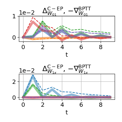
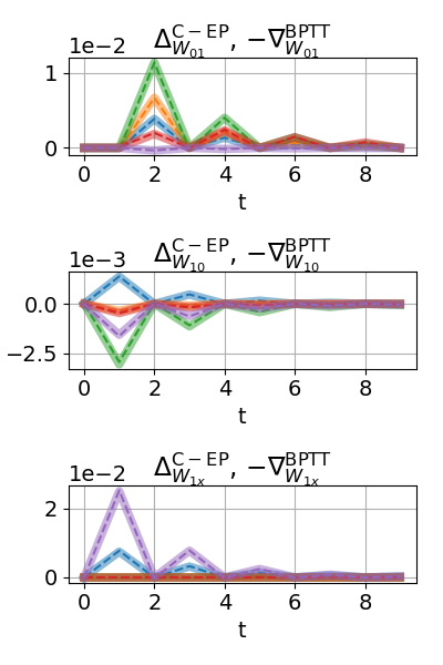
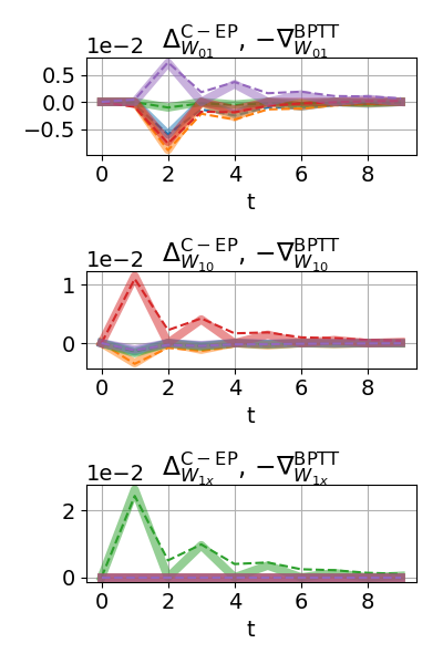
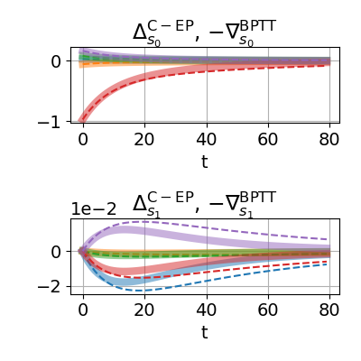
Depending on whether the updates occur continuously during the second phase and the system obey general dynamics with untied forward and backward weights, we can span a large range of deviations from the ideal conditions of Theorem 1. Fig. 5 (b) qualitatively depicts these deviations with a model for which the normalized updates of EP match the gradients of BPTT (EP) ; with continual weight updates, the normalized updates and gradients start splitting apart (C-EP), and even more so if the weights are untied (C-VF).

Protocol.

In order to create these deviations from Theorem 1 and study the consequences in terms of training, we proceed as follows. For each C-VF simulations, we tune the initial angle between forward weights (θfsubscript𝜃f\theta_{\rm f}) and backward weights (θbsubscript𝜃b\theta_{\rm b}) between 0 and 180. We denote this angle Ψ(θf,θb)Ψsubscript𝜃fsubscript𝜃b\Psi(\theta_{\rm f},\theta_{\rm b}) - see Appendix F.1 for the angle definition and the angle tuning technique employed. For each of these weight initialization, we compute the angle between the total normalized update provided by C-VF, i.e. ΔCVF(β,η,tot)=t=0K1ΔCVF(β,η,t)superscriptΔCVF𝛽𝜂totsuperscriptsubscript𝑡0𝐾1superscriptΔCVF𝛽𝜂𝑡\Delta^{\rm C-VF}(\beta,\eta,\textrm{tot})=\sum_{t=0}^{K-1}\Delta^{\rm C-VF}(\beta,\eta,t) and the total gradient provided by BPTT, i.e. BPTT(tot)=t=0K1BPTT(t)superscriptBPTTtotsuperscriptsubscript𝑡0𝐾1superscriptBPTT𝑡\nabla^{\rm BPTT}(\textrm{tot})=\sum_{t=0}^{K-1}\nabla^{\rm BPTT}(t) on random mini-batches before training. We denote this angle Ψ(ΔCVF(tot),BPTT(tot))ΨsuperscriptΔCVFtotsuperscriptBPTTtot\Psi\left(\Delta^{\rm C-VF}(\textrm{tot}),-\nabla^{\rm BPTT}(\textrm{tot})\right). Finally for each weight initialization, we perform training in the discrete-time setting of Ernoult et al. (2019) - see Appendix E.4 for model details. We proceed in the same way for EP and C-EP simulations, computing Ψ(ΔEP(tot),BPTT(tot))ΨsuperscriptΔEPtotsuperscriptBPTTtot\Psi\left(\Delta^{\rm EP}(\textrm{tot}),-\nabla^{\rm BPTT}(\textrm{tot})\right) and Ψ(ΔCEP(tot),BPTT(tot))ΨsuperscriptΔCEPtotsuperscriptBPTTtot\Psi\left(\Delta^{\rm C-EP}(\textrm{tot}),-\nabla^{\rm BPTT}(\textrm{tot})\right) before training. We use the generic notation Δ(tot)Δtot\Delta(\textrm{tot}) to denote the total normalized update. This procedure yields (x,y)𝑥𝑦(x,y) data points with x=Ψ(Δ(tot),BPTT(tot))𝑥ΨΔtotsuperscriptBPTTtotx=\Psi\left(\Delta(\textrm{tot}),-\nabla^{\rm BPTT}(\textrm{tot})\right) and y=test error𝑦test errory=\text{test error}, which are reported on Fig. 5 (a) - see Appendix F.1 for the full table of results.

Results.

Fig. 5 (a) shows the test error achieved on MNIST by EP, C-EP on the vanilla RNN with symmetric weights and C-VF on the vanilla RNN with asymmetric weights for different number of hidden layers as a function of the angle Ψ(Δ(tot),BPTT(tot))ΨΔtotsuperscriptBPTTtot\Psi\left(\Delta(\textrm{tot}),-\nabla^{\rm BPTT}(\textrm{tot})\right) before training. This graphical representation spreads the algorithms between EP which best satisfies the GDD property (leftmost point in green at 20similar-toabsentsuperscript20\sim 20^{\circ}) to C-VF which satisfies the less the GDD property (rightmost points in red and orange at 100similar-toabsentsuperscript100\sim 100^{\circ}). As expected, high angles between gradients of C-VF and BPTT lead to high error rates that can reach 90%percent9090\% for Ψ(ΔCVF(tot),BPTT(tot))ΨsuperscriptΔCVFtotsuperscriptBPTTtot\Psi\left(\Delta^{\rm C-VF}(\textrm{tot}),-\nabla^{\rm BPTT}(\textrm{tot})\right) over 100superscript100100^{\circ}. More precisely, the inset of Fig. 5 shows the same data but focusing only on results generated by initial weight angles lying below 90superscript9090^{\circ}, i.e. Ψ(θf,θb)={0,22.5,45,67.5,90}Ψsubscript𝜃fsubscript𝜃bsuperscript0superscript22.5superscript45superscript67.5superscript90\Psi(\theta_{\rm f},\theta_{\rm b})=\{0^{\circ},22.5^{\circ},45^{\circ},67.5^{\circ},90^{\circ}\}. From standard EP with one hidden layer to C-VF with two hidden layers, the test error increases monotonically with Ψ(Δ(tot),BPTT(tot))ΨΔtotsuperscriptBPTTtot\Psi\left(\Delta(\textrm{tot}),-\nabla^{\rm BPTT}(\textrm{tot})\right) but does not exceed 5.05%percent5.055.05\% on average. This result confirms the importance of proper weight initialization when weights are untied, also discussed in other context (Lillicrap et al., 2016). When the initial weight angle is of 0superscript00^{\circ}, the impact of untying the weights on classification accuracy remains constrained, as shown in table of Fig. 4. Upon untying the forward and backward weights, the test error increases by 0.2%similar-toabsentpercent0.2\sim 0.2\% with one hidden layer and by 0.5%similar-toabsentpercent0.5\sim 0.5\% with two hidden layers compared to standard C-EP.

Refer to caption
Refer to caption
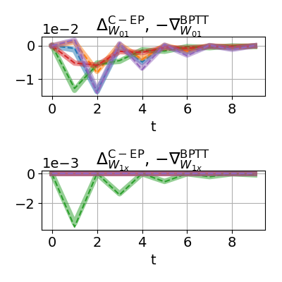
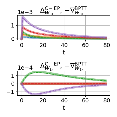
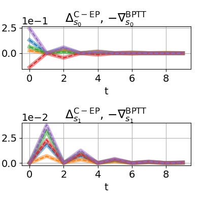
Figure 5: Three versions of EP: standard Equilibrium Propagation (EP), Continual Equilibrium Propagation (C-EP) and Continual Vector Field EP (C-VF). ##\#-h denotes the number of hidden layers. (a): test error rate on MNIST as a function of the initial angle ΨΨ\Psi between the total normalized update of EP and the total gradient of BPTT. (b): Dashed and continuous lines respectively represent the normalized updates Δθ(t)subscriptΔ𝜃𝑡\Delta_{\theta}(t) (i.e. ΔθEP(t)superscriptsubscriptΔ𝜃EP𝑡\Delta_{\theta}^{\rm EP}(t), ΔθCEP(t)superscriptsubscriptΔ𝜃CEP𝑡\Delta_{\theta}^{\rm C-EP}(t), ΔθCVF(t)superscriptsubscriptΔ𝜃CVF𝑡\Delta_{\theta}^{\rm C-VF}(t)) and the gradients θBPTT(t)superscriptsubscript𝜃BPTT𝑡-\nabla_{\theta}^{\rm BPTT}(t). Each randomly selected synapse corresponds to one color. While dashed and continuous lines coincide for standard EP, they split apart upon untying the weights and using continual updates.

5 Discussion

Equilibrium Propagation is an algorithm that leverages the dynamical nature of neurons to compute weight gradients through the physics of the neural network. C-EP embraces simultaneous synapse and neuron dynamics, getting rid of the need for artificial memory units for storing the neuron values between different phases. The C-EP framework preserves the equivalence with Backpropagation Through Time: in the limit of sufficiently slow synaptic dynamics (i.e. small learning rates), the system satisfies Gradient Descending Dynamics (Theorem 1). Our experimental results confirm this theorem. When training our vanilla RNN with symmetric weights with C-EP while ensuring convergence in 100 epochs, a modest reduction in MNIST accuracy is seen with regards to standard EP. This accuracy reduction can be eliminated by using smaller learning rates and rescaling up the total weight update at the end of the second phase (Appendix F.2). On top of extending the theory of Ernoult et al. (2019), Theorem 1 also appears to provide a statistically robust approach for C-EP based learning: our experimental results show as in Ernoult et al. (2019) that, for a given network with specified neuron and synapse dynamics, the more the updates of Equilibrium Propagation follow the gradients provided by Backpropagation Through Time before training (in terms of angle between weight vectors, in this work), the better this network can learn. Specifically, Fig. 5 (a) shows that hyperparameters should be tuned so that before training, C-EP updates stay within 90superscript9090^{\circ} of the gradients provided by BPTT. In practice, it amounts to tune the degree of symmetry of the dynamics, for instance the angle between forward and backward weights - see Fig. 4.

Our C-EP and C-VF algorithms exhibit features reminiscent of biology. C-VF extends C-EP training to RNNs with asymmetric weights between neurons, as is the case in biology. Its learning rule, local in space and time, is furthermore closely acquainted to Spike Timing Dependent Plasticity (STDP), a learning rule widely studied in neuroscience, inferred in vitro and in vivo from neural recordings in the hippocampus (Dan and Poo, 2004). In STDP, the synaptic strength is modulated by the relative timings of pre and post synaptic spikes within a precise time window (Bi and Poo, 1998; 2001). Strikingly, the same rule that we use for C-VF learning can approximate STDP correlations in a rate-based formulation, as shown through numerical experiments by Bengio et al. (2015). From this viewpoint, our work brings EP a step closer to biology. This being said, C-EP and C-VF do not aim at being end-to-end models of biological learning. EP and its variants are meant to optimize any given loss function, and this loss function could be for supervised learning (as in our experiments) or for any differentiable loss function in general. The core motivation of this work is to focus on and propose a fully local implementation of EP, in particular to foster its hardware implementation. When computed on a standard computer, due to the use of small learning rates to mimic analog dynamics within a finite number of epochs, training our models with C-EP and C-VF entail long simulation times. With a Titan RTX GPU, training a fully connected architecture on MNIST takes 2 hours 39 mins with 1 hidden layer and 10 hours 49 mins with 2 hidden layers. On the other hand, C-EP and C-VF might be particularly efficient in terms of speed and energy consumption when operated on neuromorphic hardware that employs analog device physics (Ambrogio et al., 2018; Romera et al., 2018). To this purpose, our work can provide an engineering guidance to map Equilibrium Propagation onto a neuromorphic system. This is one step towards bridging Equilibrium Propagation with neuromorphic computing and thereby energy efficient hardware implementations of gradient-based learning algorithms.

References

  • Ackley et al. [1985] D. H. Ackley, G. E. Hinton, and T. J. Sejnowski. A learning algorithm for boltzmann machines. Cognitive science, 9(1):147–169, 1985.
  • Almeida [1987] L. B. Almeida. A learning rule for asynchronous perceptrons with feedback in a combinatorial environment. volume 2, pages 609–618, San Diego 1987, 1987. IEEE, New York.
  • Almeida [1990] L. B. Almeida. A learning rule for asynchronous perceptrons with feedback in a combinatorial environment. In Artificial neural networks: concept learning, pages 102–111. 1990.
  • Ambrogio et al. [2018] S. Ambrogio, P. Narayanan, H. Tsai, R. M. Shelby, I. Boybat, C. Nolfo, S. Sidler, M. Giordano, M. Bodini, N. C. Farinha, et al. Equivalent-accuracy accelerated neural-network training using analogue memory. Nature, 558(7708):60, 2018.
  • Bengio et al. [2015] Y. Bengio, T. Mesnard, A. Fischer, S. Zhang, and Y. Wu. Stdp as presynaptic activity times rate of change of postsynaptic activity. arXiv preprint arXiv:1509.05936, 2015.
  • Bi and Poo [1998] G.-q. Bi and M.-m. Poo. Synaptic modifications in cultured hippocampal neurons: dependence on spike timing, synaptic strength, and postsynaptic cell type. Journal of neuroscience, 18(24):10464–10472, 1998.
  • Bi and Poo [2001] G.-q. Bi and M.-m. Poo. Synaptic modification by correlated activity: Hebb’s postulate revisited. Annual review of neuroscience, 24(1):139–166, 2001.
  • Dan and Poo [2004] Y. Dan and M.-m. Poo. Spike timing-dependent plasticity of neural circuits. Neuron, 44(1):23–30, 2004.
  • Ernoult et al. [2019] M. Ernoult, J. Grollier, D. Querlioz, Y. Bengio, and B. Scellier. Updates of equilibrium prop match gradients of backprop through time in an rnn with static input. arXiv preprint arXiv:1905.13633, 2019.
  • Hertz [2018] J. A. Hertz. Introduction to the theory of neural computation. CRC Press, 2018.
  • Hinton [2002] G. E. Hinton. Training products of experts by minimizing contrastive divergence. Neural computation, 14(8):1771–1800, 2002.
  • LeCun et al. [2015] Y. LeCun, Y. Bengio, and G. Hinton. Deep learning. Nature, 521(7553):436, 2015.
  • Lillicrap et al. [2016] T. P. Lillicrap, D. Cownden, D. B. Tweed, and C. J. Akerman. Random synaptic feedback weights support error backpropagation for deep learning. Nature communications, 7:13276, 2016.
  • Movellan [1991] J. R. Movellan. Contrastive hebbian learning in the continuous hopfield model. In Connectionist models, pages 10–17. Elsevier, 1991.
  • Pineda [1987a] F. J. Pineda. Generalization of back-propagation to recurrent neural networks. 59:2229–2232, 1987a.
  • Pineda [1987b] F. J. Pineda. Generalization of back-propagation to recurrent neural networks. Physical review letters, 59(19):2229, 1987b.
  • Romera et al. [2018] M. Romera, P. Talatchian, S. Tsunegi, F. A. Araujo, V. Cros, P. Bortolotti, J. Trastoy, K. Yakushiji, A. Fukushima, H. Kubota, et al. Vowel recognition with four coupled spin-torque nano-oscillators. Nature, 563(7730):230, 2018.
  • Scellier and Bengio [2017] B. Scellier and Y. Bengio. Equilibrium propagation: Bridging the gap between energy-based models and backpropagation. Frontiers in computational neuroscience, 11, 2017.
  • Scellier and Bengio [2019] B. Scellier and Y. Bengio. Equivalence of equilibrium propagation and recurrent backpropagation. Neural computation, 31(2):312–329, 2019.
  • Scellier et al. [2018] B. Scellier, A. Goyal, J. Binas, T. Mesnard, and Y. Bengio. Generalization of equilibrium propagation to vector field dynamics. arXiv preprint arXiv:1808.04873, 2018.
  • Strubell et al. [2019] E. Strubell, A. Ganesh, and A. McCallum. Energy and policy considerations for deep learning in nlp. arXiv preprint arXiv:1906.02243, 2019.

Appendix

Appendix A Proof of Theorem 1

In this appendix, we prove Theorem 1, which we recall here.

See 1

A.1 A Spectrum of Four Computationally Equivalent Learning Algorithms

Proving Theorem 1 amounts to prove the equivalence of C-EP and BPTT. In fact we can prove the equivalence of four algorithms, which all compute the gradient of the loss:

  1. 1.

    Backpropagation Through Time (BPTT), presented in Section B.2,

  2. 2.

    Recurrent Backpropagation (RBP), presented in Section B.3,

  3. 3.

    Equilibrium Propagation (EP), presented in Section 2,

  4. 4.

    Equilibrium Propagation with Continual Weight Updates (C-EP), introduced in Section 3.

In this spectrum of algorithms, BPTT is the most practical algorithm to date from the point of view of machine learning, but also the less biologically realistic. In contrast, C-EP is the most realistic in terms of implementation in biological systems, while it is to date the least practical and least efficient for conventional machine learning (computations on standard Von-Neumann hardware are considerably slower due to repeated parameter updates, requiring memory access at each time-step of the second phase).

A.2 Sketch of the Proof

Theorem 1 can be proved in three phases, using the following three lemmas.

Lemma 2 (Equivalence of C-EP and EP).

In the limit of small learning rate, i.e. η0𝜂0\eta\to 0, the (normalized) updates of C-EP are equal to those of EP:

t0:{limη0(η>0)ΔsCEP(β,η,t)=ΔsEP(β,t),limη0(η>0)ΔθCEP(β,η,t)=ΔθEP(β,t).:for-all𝑡0casessubscript𝜂0𝜂0superscriptsubscriptΔ𝑠CEP𝛽𝜂𝑡superscriptsubscriptΔ𝑠EP𝛽𝑡subscript𝜂0𝜂0superscriptsubscriptΔ𝜃CEP𝛽𝜂𝑡superscriptsubscriptΔ𝜃EP𝛽𝑡\forall t\geq 0:\left\{\begin{array}[]{l}\displaystyle\lim_{\eta\to 0\;(\eta>0)}\;\Delta_{s}^{\rm C-EP}(\beta,\eta,t)=\Delta_{s}^{\rm EP}(\beta,t),\\ \displaystyle\lim_{\eta\to 0\;(\eta>0)}\;\Delta_{\theta}^{\rm C-EP}(\beta,\eta,t)=\Delta_{\theta}^{\rm EP}(\beta,t).\end{array}\right. (15)
Lemma 3 (Equivalence of EP and RBP).

Assume that the transition function derives from a primitive function, i.e. that F𝐹F is of the form F(x,s,θ)=Φs(x,s,θ)𝐹𝑥𝑠𝜃Φ𝑠𝑥𝑠𝜃F\left(x,s,\theta\right)=\frac{\partial\Phi}{\partial s}\left(x,s,\theta\right). Then, in the limit of small hyperparameter β𝛽\beta, the normalized updates of EP are equal to the gradients of RBP:

t0:{limβ0(β>0)ΔsEP(β,t)=sRBP(t),limβ0(β>0)ΔθEP(β,t)=θRBP(t).:for-all𝑡0casessubscript𝛽0𝛽0subscriptsuperscriptΔEP𝑠𝛽𝑡superscriptsubscript𝑠RBP𝑡subscript𝛽0𝛽0subscriptsuperscriptΔEP𝜃𝛽𝑡superscriptsubscript𝜃RBP𝑡\forall t\geq 0:\left\{\begin{array}[]{l}\displaystyle\lim_{\beta\to 0\;(\beta>0)}\;\Delta^{\rm EP}_{s}(\beta,t)=-\nabla_{s}^{\rm RBP}(t),\\ \displaystyle\lim_{\beta\to 0\;(\beta>0)}\;\Delta^{\rm EP}_{\theta}(\beta,t)=-\nabla_{\theta}^{\rm RBP}(t).\end{array}\right. (16)
Lemma 4 (Equivalence of BPTT and RBP).

In the setting with static input x𝑥x, suppose that the network has reached the steady state ssubscript𝑠s_{*} after TK𝑇𝐾T-K steps, i.e. sTK=sTK+1==sT1=sT=ssubscript𝑠𝑇𝐾subscript𝑠𝑇𝐾1subscript𝑠𝑇1subscript𝑠𝑇subscript𝑠s_{T-K}=s_{T-K+1}=\cdots=s_{T-1}=s_{T}=s_{*}. Then the first K𝐾K gradients of BPTT are equal to the first K gradient of RBP, i.e.

t=0,1,,K:{sBPTT(t)=sRBP(t),θBPTT(t)=θRBP(t).:for-all𝑡01𝐾casessuperscriptsubscript𝑠BPTT𝑡superscriptsubscript𝑠RBP𝑡superscriptsubscript𝜃BPTT𝑡superscriptsubscript𝜃RBP𝑡\forall t=0,1,\ldots,K:\left\{\begin{array}[]{l}\displaystyle\nabla_{s}^{\rm BPTT}(t)=\nabla_{s}^{\rm RBP}(t),\\ \displaystyle\nabla_{\theta}^{\rm BPTT}(t)=\nabla_{\theta}^{\rm RBP}(t).\end{array}\right. (17)

Proofs of the Lemmas can be found in the following places:

  • The link between BPTT and RBP (Lemma 2) is known since the late 1980s and can be found e.g. in Hertz [2018]. We also prove it here in Appendix B.

  • Lemma 3 was proved in Scellier and Bengio [2019] in the setting of real-time dynamics.

  • Lemma 4 is the new ingredient contributed here, and we prove it in Appendix A.3.

Also a direct proof of the equivalence of EP and BPTT was derived in Ernoult et al. [2019].

A.3 Equivalence of C-EP and EP

First, recall the dynamics of C-EP in the second phase: starting from s0β,η=ssuperscriptsubscript𝑠0𝛽𝜂subscript𝑠s_{0}^{\beta,\eta}=s_{*} and θ0β,η=θsuperscriptsubscript𝜃0𝛽𝜂𝜃\theta_{0}^{\beta,\eta}=\theta we have

t0:{st+1β,η=Φs(x,stβ,η,θtβ,η)βs(stβ,η,y),θt+1β,η=θtβ,η+ηβ(Φθ(x,st+1β,η,θtβ,η)Φθ(x,stβ,η,θtβ,η)).:for-all𝑡0casessuperscriptsubscript𝑠𝑡1𝛽𝜂Φ𝑠𝑥superscriptsubscript𝑠𝑡𝛽𝜂superscriptsubscript𝜃𝑡𝛽𝜂𝛽𝑠superscriptsubscript𝑠𝑡𝛽𝜂𝑦superscriptsubscript𝜃𝑡1𝛽𝜂superscriptsubscript𝜃𝑡𝛽𝜂𝜂𝛽Φ𝜃𝑥superscriptsubscript𝑠𝑡1𝛽𝜂superscriptsubscript𝜃𝑡𝛽𝜂Φ𝜃𝑥superscriptsubscript𝑠𝑡𝛽𝜂superscriptsubscript𝜃𝑡𝛽𝜂\forall t\geq 0:\left\{\begin{array}[]{l}\displaystyle s_{t+1}^{\beta,\eta}=\frac{\partial\Phi}{\partial s}\left(x,s_{t}^{\beta,\eta},\theta_{t}^{\beta,\eta}\right)-\beta\;\frac{\partial\ell}{\partial s}\left(s_{t}^{\beta,\eta},y\right),\\ \displaystyle\theta_{t+1}^{\beta,\eta}=\theta_{t}^{\beta,\eta}+\frac{\eta}{\beta}\left(\frac{\partial\Phi}{\partial\theta}\left(x,s_{t+1}^{\beta,\eta},\theta_{t}^{\beta,\eta}\right)-\frac{\partial\Phi}{\partial\theta}\left(x,s_{t}^{\beta,\eta},\theta_{t}^{\beta,\eta}\right)\right).\end{array}\right. (18)

We have also defined the normalized updates of C-EP:

t0:{ΔsCEP(β,η,t)=1β(st+1β,ηstβ,η),ΔθCEP(β,η,t)=1η(θt+1β,ηθtβ,η).:for-all𝑡0casessuperscriptsubscriptΔ𝑠CEP𝛽𝜂𝑡1𝛽superscriptsubscript𝑠𝑡1𝛽𝜂superscriptsubscript𝑠𝑡𝛽𝜂superscriptsubscriptΔ𝜃CEP𝛽𝜂𝑡1𝜂superscriptsubscript𝜃𝑡1𝛽𝜂superscriptsubscript𝜃𝑡𝛽𝜂\forall t\geq 0:\left\{\begin{array}[]{l}\displaystyle\Delta_{s}^{\rm C-EP}(\beta,\eta,t)=\frac{1}{\beta}\left(s_{t+1}^{\beta,\eta}-s_{t}^{\beta,\eta}\right),\\ \displaystyle\Delta_{\theta}^{\rm C-EP}(\beta,\eta,t)=\frac{1}{\eta}\left(\theta_{t+1}^{\beta,\eta}-\theta_{t}^{\beta,\eta}\right).\end{array}\right. (19)

We also recall the dynamics of EP in the second phase:

s0β=sandst+1β=Φs(x,stβ,θ)βs(stβ,y),formulae-sequencesuperscriptsubscript𝑠0𝛽subscript𝑠andsuperscriptsubscript𝑠𝑡1𝛽Φ𝑠𝑥superscriptsubscript𝑠𝑡𝛽𝜃𝛽𝑠superscriptsubscript𝑠𝑡𝛽𝑦s_{0}^{\beta}=s_{*}\quad\text{and}\quad s_{t+1}^{\beta}=\frac{\partial\Phi}{\partial s}\left(x,s_{t}^{\beta},\theta\right)-\beta\;\frac{\partial\ell}{\partial s}\left(s_{t}^{\beta},y\right), (20)

as well as the normalized updates of EP, as defined in Ernoult et al. [2019]:

t0:{ΔsEP(β,t)=1β(st+1βstβ),ΔθEP(β,t)=1β(Φθ(x,st+1β,θ)Φθ(x,stβ,θ)).:for-all𝑡0casessuperscriptsubscriptΔ𝑠EP𝛽𝑡1𝛽superscriptsubscript𝑠𝑡1𝛽superscriptsubscript𝑠𝑡𝛽superscriptsubscriptΔ𝜃EP𝛽𝑡1𝛽Φ𝜃𝑥superscriptsubscript𝑠𝑡1𝛽𝜃Φ𝜃𝑥superscriptsubscript𝑠𝑡𝛽𝜃\forall t\geq 0:\left\{\begin{array}[]{l}\displaystyle\Delta_{s}^{\rm EP}(\beta,t)=\frac{1}{\beta}\left(s_{t+1}^{\beta}-s_{t}^{\beta}\right),\\ \displaystyle\Delta_{\theta}^{\rm EP}(\beta,t)=\frac{1}{\beta}\left(\frac{\partial\Phi}{\partial\theta}\left(x,s_{t+1}^{\beta},\theta\right)-\frac{\partial\Phi}{\partial\theta}\left(x,s_{t}^{\beta},\theta\right)\right).\end{array}\right. (21)

See 2

Proof of Lemma 2.

We want to compute the limits of ΔsCEP(β,η,t)superscriptsubscriptΔ𝑠CEP𝛽𝜂𝑡\Delta_{s}^{\rm C-EP}(\beta,\eta,t) and ΔθCEP(β,η,t)superscriptsubscriptΔ𝜃CEP𝛽𝜂𝑡\Delta_{\theta}^{\rm C-EP}(\beta,\eta,t) as η0𝜂0\eta\to 0 with η>0𝜂0\eta>0. First of all, note that under mild assumptions – which we made here – of regularity on the functions ΦΦ\Phi and \ell (e.g. continuous differentiability), for fixed t𝑡t and β𝛽\beta, the quantities stβ,ηsuperscriptsubscript𝑠𝑡𝛽𝜂s_{t}^{\beta,\eta} and θtβ,ηsuperscriptsubscript𝜃𝑡𝛽𝜂\theta_{t}^{\beta,\eta} are continuous as functions of η𝜂\eta ; this is straightforward from the form of Eq. (18). As a consequence, ΔsCEP(β,η,t)superscriptsubscriptΔ𝑠CEP𝛽𝜂𝑡\Delta_{s}^{\rm C-EP}(\beta,\eta,t) is a continuous function of η𝜂\eta, which implies in particular that

limη0(η>0)ΔsCEP(β,η,t)=ΔsCEP(β,0,t).subscript𝜂0𝜂0superscriptsubscriptΔ𝑠CEP𝛽𝜂𝑡superscriptsubscriptΔ𝑠CEP𝛽0𝑡\lim_{\eta\to 0\;(\eta>0)}\;\Delta_{s}^{\rm C-EP}(\beta,\eta,t)=\Delta_{s}^{\rm C-EP}(\beta,0,t). (22)

Now, taking η=0𝜂0\eta=0 in the bottom equation of Eq. (18) yields the recurrence relation θt+1β,0=θtβ,0superscriptsubscript𝜃𝑡1𝛽0superscriptsubscript𝜃𝑡𝛽0\theta_{t+1}^{\beta,0}=\theta_{t}^{\beta,0}, so that θtβ,0=θ0β,0=θsuperscriptsubscript𝜃𝑡𝛽0superscriptsubscript𝜃0𝛽0𝜃\theta_{t}^{\beta,0}=\theta_{0}^{\beta,0}=\theta for every t𝑡t. Injecting θtβ,0=θsuperscriptsubscript𝜃𝑡𝛽0𝜃\theta_{t}^{\beta,0}=\theta in the top equation of Eq. (18) yields for stβ,0superscriptsubscript𝑠𝑡𝛽0s_{t}^{\beta,0} the same recurrence relation as that of stβsuperscriptsubscript𝑠𝑡𝛽s_{t}^{\beta} (Eq. 20), so that stβ,0=stβsuperscriptsubscript𝑠𝑡𝛽0superscriptsubscript𝑠𝑡𝛽s_{t}^{\beta,0}=s_{t}^{\beta} for every t𝑡t. Therefore, for η=0𝜂0\eta=0, we have

ΔsCEP(β,0,t)=1β(st+1β,0stβ,0)=1β(st+1βstβ)=ΔsEP(β,t).superscriptsubscriptΔ𝑠CEP𝛽0𝑡1𝛽superscriptsubscript𝑠𝑡1𝛽0superscriptsubscript𝑠𝑡𝛽01𝛽superscriptsubscript𝑠𝑡1𝛽superscriptsubscript𝑠𝑡𝛽superscriptsubscriptΔ𝑠EP𝛽𝑡\Delta_{s}^{\rm C-EP}(\beta,0,t)=\frac{1}{\beta}\left(s_{t+1}^{\beta,0}-s_{t}^{\beta,0}\right)=\frac{1}{\beta}\left(s_{t+1}^{\beta}-s_{t}^{\beta}\right)=\Delta_{s}^{\rm EP}(\beta,t). (23)

It follows from Eq. (22) and Eq. (23) that

limη0(η>0)ΔsCEP(β,η,t)=ΔsEP(β,t).subscript𝜂0𝜂0superscriptsubscriptΔ𝑠CEP𝛽𝜂𝑡superscriptsubscriptΔ𝑠EP𝛽𝑡\lim_{\eta\to 0\;(\eta>0)}\;\Delta_{s}^{\rm C-EP}(\beta,\eta,t)=\Delta_{s}^{\rm EP}(\beta,t). (24)

Now let us compute limη0(η>0)ΔsCEP(β,η,t)subscript𝜂0𝜂0superscriptsubscriptΔ𝑠CEP𝛽𝜂𝑡\lim_{\eta\to 0\;(\eta>0)}\;\Delta_{s}^{\rm C-EP}(\beta,\eta,t). Using Eq. (18), we have

ΔθCEP(β,η,t)superscriptsubscriptΔ𝜃CEP𝛽𝜂𝑡\displaystyle\Delta_{\theta}^{\rm C-EP}(\beta,\eta,t) =1η(θt+1β,ηθtβ,η)absent1𝜂superscriptsubscript𝜃𝑡1𝛽𝜂superscriptsubscript𝜃𝑡𝛽𝜂\displaystyle=\frac{1}{\eta}\left(\theta_{t+1}^{\beta,\eta}-\theta_{t}^{\beta,\eta}\right) (25)
=1β(Φθ(x,st+1β,η,θtβ,η)Φθ(x,stβ,η,θtβ,η)).absent1𝛽Φ𝜃𝑥superscriptsubscript𝑠𝑡1𝛽𝜂superscriptsubscript𝜃𝑡𝛽𝜂Φ𝜃𝑥superscriptsubscript𝑠𝑡𝛽𝜂superscriptsubscript𝜃𝑡𝛽𝜂\displaystyle=\frac{1}{\beta}\left(\frac{\partial\Phi}{\partial\theta}\left(x,s_{t+1}^{\beta,\eta},\theta_{t}^{\beta,\eta}\right)-\frac{\partial\Phi}{\partial\theta}\left(x,s_{t}^{\beta,\eta},\theta_{t}^{\beta,\eta}\right)\right). (26)

Similarly as before, for fixed t𝑡t, Φθ(x,stβ,η,θtβ,η)Φ𝜃𝑥superscriptsubscript𝑠𝑡𝛽𝜂superscriptsubscript𝜃𝑡𝛽𝜂\frac{\partial\Phi}{\partial\theta}\left(x,s_{t}^{\beta,\eta},\theta_{t}^{\beta,\eta}\right) is a continuous function of η𝜂\eta. Therefore

limη0(η>0)ΔθCEP(β,η,t)subscript𝜂0𝜂0superscriptsubscriptΔ𝜃CEP𝛽𝜂𝑡\displaystyle\lim_{\eta\to 0\;(\eta>0)}\;\Delta_{\theta}^{\rm C-EP}(\beta,\eta,t) =1β(Φθ(x,st+1β,0,θtβ,0)Φθ(x,stβ,0,θtβ,0))absent1𝛽Φ𝜃𝑥superscriptsubscript𝑠𝑡1𝛽0superscriptsubscript𝜃𝑡𝛽0Φ𝜃𝑥superscriptsubscript𝑠𝑡𝛽0superscriptsubscript𝜃𝑡𝛽0\displaystyle=\frac{1}{\beta}\left(\frac{\partial\Phi}{\partial\theta}\left(x,s_{t+1}^{\beta,0},\theta_{t}^{\beta,0}\right)-\frac{\partial\Phi}{\partial\theta}\left(x,s_{t}^{\beta,0},\theta_{t}^{\beta,0}\right)\right) (27)
=1β(Φθ(x,st+1β,θ)Φθ(x,stβ,θ))=ΔθEP(β,t).absent1𝛽Φ𝜃𝑥superscriptsubscript𝑠𝑡1𝛽𝜃Φ𝜃𝑥superscriptsubscript𝑠𝑡𝛽𝜃superscriptsubscriptΔ𝜃EP𝛽𝑡\displaystyle=\frac{1}{\beta}\left(\frac{\partial\Phi}{\partial\theta}\left(x,s_{t+1}^{\beta},\theta\right)-\frac{\partial\Phi}{\partial\theta}\left(x,s_{t}^{\beta},\theta\right)\right)=\Delta_{\theta}^{\rm EP}(\beta,t). (28)

A consequence of Lemma 2 is that the total update of C-EP matches the total update of EP in the limit of small η𝜂\eta, so that we retrieve the standard EP learning rule of Eq. (4). More explicitly, after K steps in the second phase and starting from θ0β,η=θ0superscriptsubscript𝜃0𝛽𝜂subscript𝜃0\theta_{0}^{\beta,\eta}=\theta_{0}:

θKβ,ηθ0superscriptsubscript𝜃𝐾𝛽𝜂subscript𝜃0\displaystyle\theta_{K}^{\beta,\eta}-\theta_{0} =t=0K1θt+1β,ηθtβ,ηabsentsuperscriptsubscript𝑡0𝐾1superscriptsubscript𝜃𝑡1𝛽𝜂superscriptsubscript𝜃𝑡𝛽𝜂\displaystyle=\sum_{t=0}^{K-1}\theta_{t+1}^{\beta,\eta}-\theta_{t}^{\beta,\eta}
=t=0K1ηΔθCEP(β,η,t)(definition of ΔθCEP, Eq. (9))absentsuperscriptsubscript𝑡0𝐾1𝜂superscriptsubscriptΔ𝜃CEP𝛽𝜂𝑡(definition of ΔθCEP, Eq. (9))\displaystyle=\sum_{t=0}^{K-1}\eta\Delta_{\theta}^{\rm C-EP}(\beta,\eta,t)\qquad\mbox{(definition of $\Delta_{\theta}^{\rm C-EP}$, Eq.~{}(\ref{eq:updates-cep}))}
η0t=0K1ηΔθEP(β,t)(Lemma 2)greater-than-or-equivalent-to𝜂0superscriptsubscript𝑡0𝐾1𝜂superscriptsubscriptΔ𝜃EP𝛽𝑡(Lemma 2)\displaystyle\underset{\eta\gtrsim 0}{\approx}\sum_{t=0}^{K-1}\eta\Delta_{\theta}^{\rm EP}(\beta,t)\qquad\mbox{(Lemma~{}\ref{lma:ep-cep})}
=t=0K1η1β(Φθ(x,st+1,θ0)Φθ(x,st+1,θ0))(definition of ΔθEP, Eq. (21))absentsuperscriptsubscript𝑡0𝐾1𝜂1𝛽Φ𝜃𝑥subscript𝑠𝑡1subscript𝜃0Φ𝜃𝑥subscript𝑠𝑡1subscript𝜃0(definition of ΔθEP, Eq. (21))\displaystyle=\sum_{t=0}^{K-1}\eta\frac{1}{\beta}\left(\frac{\partial\Phi}{\partial\theta}(x,s_{t+1},\theta_{0})-\frac{\partial\Phi}{\partial\theta}(x,s_{t+1},\theta_{0})\right)\qquad\mbox{(definition of $\Delta_{\theta}^{\rm EP}$, Eq.~{}(\ref{eq:ep-updates}))}
=ηβ(Φθ(x,sKβ,θ0)Φθ(x,s,θ0))absent𝜂𝛽Φ𝜃𝑥superscriptsubscript𝑠𝐾𝛽subscript𝜃0Φ𝜃𝑥subscript𝑠subscript𝜃0\displaystyle=\frac{\eta}{\beta}\left(\frac{\partial\Phi}{\partial\theta}(x,s_{K}^{\beta},\theta_{0})-\frac{\partial\Phi}{\partial\theta}(x,s_{*},\theta_{0})\right)

Appendix B Equivalence of BPTT and RBP

In this section, we recall Backprop Through Time (BPTT) and the Almeida-Pineda Recurrent Backprop (RBP) algorithm, which can both be used to optimize the loss superscript{\mathcal{L}}^{*} of Eq. 3. Historically, BPTT and RBP were invented separately around the same time. RBP was introduced at a time when convergent RNNs (such as the one studied in this paper) were popular. Nowadays, convergent RNNs are less popular ; in the field of deep learning, RNNs are almost exclusively used for tasks that deal with sequential data and BPTT is the algorithm of choice to train such RNNs. Here, we present RBP in a way that it can be seen as a particular case of BPTT.

B.1 Sketch of the Proof of Lemma 4

Lemma 4, which we recall here, is a consequence of Proposition 5 and Definition 6 below.

See 4

However, in general, the gradients BPTT(t)superscriptBPTT𝑡\nabla^{\rm BPTT}(t) of BPTT and the gradients RBP(t)superscriptRBP𝑡\nabla^{\rm RBP}(t) of RBP are not equal for t>K𝑡𝐾t>K. This is because BPTT and RBP compute the gradients of different loss functions:

  • BPTT computes the gradient of the loss after T𝑇T time steps, i.e. =(sT,y)subscript𝑠𝑇𝑦{\mathcal{L}}=\ell\left(s_{T},y\right),

  • RBP computes the gradients of the loss at the steady state, i.e. =(s,y)superscriptsubscript𝑠𝑦{\mathcal{L}^{*}}=\ell\left(s_{*},y\right).

B.2 Backpropagation Through Time (BPTT)

Backpropagation Through Time (BPTT) is the standard method to train RNNs and can also be used to train the kind of convergent RNNs that we study in this paper. To this end, we consider the cost of the state sTsubscript𝑠𝑇s_{T} after T𝑇T time steps, denoted =(sT,y)subscript𝑠𝑇𝑦{\mathcal{L}}=\ell\left(s_{T},y\right), and we substitute the loss after T𝑇T time steps {\mathcal{L}} as a proxy for the loss at the steady state =(s,y)superscriptsubscript𝑠𝑦{\mathcal{L}^{*}}=\ell\left(s_{*},y\right). The gradients of {\mathcal{L}} can then be computed with BPTT.

To do this, we recall some of the inner working mechanisms of BPTT. Eq. (1) rewrites in the form st+1=F(x,st,θt+1=θ)subscript𝑠𝑡1𝐹𝑥subscript𝑠𝑡subscript𝜃𝑡1𝜃s_{t+1}=F\left(x,s_{t},\theta_{t+1}=\theta\right), where θtsubscript𝜃𝑡\theta_{t} denotes the parameter of the model at time step t𝑡t, the value θ𝜃\theta being shared across all time steps. This way of rewriting Eq. (1) enables us to define the partial derivative θtsubscript𝜃𝑡\frac{\partial\mathcal{L}}{\partial\theta_{t}} as the sensitivity of the loss \mathcal{L} with respect to θtsubscript𝜃𝑡\theta_{t} when θ1,θt1,θt+1,θTsubscript𝜃1subscript𝜃𝑡1subscript𝜃𝑡1subscript𝜃𝑇\theta_{1},\ldots\theta_{t-1},\theta_{t+1},\ldots\theta_{T} remain fixed (set to the value θ𝜃\theta). With these notations, the gradient θ𝜃\frac{\partial\mathcal{L}}{\partial\theta} reads as the sum:

θ=θ1+θ2++θT.𝜃subscript𝜃1subscript𝜃2subscript𝜃𝑇\frac{\partial{\mathcal{L}}}{\partial\theta}=\frac{\partial{\mathcal{L}}}{\partial\theta_{1}}+\frac{\partial{\mathcal{L}}}{\partial\theta_{2}}+\cdots+\frac{\partial{\mathcal{L}}}{\partial\theta_{T}}. (29)

BPTT computes the ’full’ gradient θ𝜃\frac{\partial{\mathcal{L}}}{\partial\theta} by first computing the partial derivatives stsubscript𝑠𝑡\frac{\partial{\mathcal{L}}}{\partial s_{t}} and θtsubscript𝜃𝑡\frac{\partial{\mathcal{L}}}{\partial\theta_{t}} iteratively, backward in time, using the chain rule of differentiation. In this work, we denote the gradients that BPTT computes:

t[0,T1]:{sBPTT(t)=sTt,θBPTT(t)=θTt.:for-all𝑡0𝑇1casessubscriptsuperscriptBPTT𝑠𝑡subscript𝑠𝑇𝑡missing-subexpressionsubscriptsuperscriptBPTT𝜃𝑡subscript𝜃𝑇𝑡missing-subexpression\displaystyle\forall t\in[0,T-1]:\left\{\begin{array}[]{ll}\displaystyle\nabla^{\rm BPTT}_{s}(t)=\frac{\partial{\mathcal{L}}}{\partial s_{T-t}},\\ \displaystyle\nabla^{\rm BPTT}_{\theta}(t)=\frac{\partial{\mathcal{L}}}{\partial\theta_{T-t}}.\end{array}\right. (32)
Proposition 5 (Gradients of BPTT).

The gradients sBPTT(t)subscriptsuperscriptBPTT𝑠𝑡\nabla^{\rm BPTT}_{s}(t) and θBPTT(t)subscriptsuperscriptBPTT𝜃𝑡\nabla^{\rm BPTT}_{\theta}(t) satisfy the recurrence relationship

sBPTT(0)subscriptsuperscriptBPTT𝑠0\displaystyle\nabla^{\rm BPTT}_{s}(0) =s(sT,y),absent𝑠subscript𝑠𝑇𝑦\displaystyle=\frac{\partial\ell}{\partial s}\left(s_{T},y\right), (33)
t=1,2,,T,sBPTT(t)for-all𝑡12𝑇subscriptsuperscriptBPTT𝑠𝑡\displaystyle\forall t=1,2,\ldots,T,\qquad\nabla^{\rm BPTT}_{s}(t) =Fs(x,sTt,θ)sBPTT(t1),absent𝐹𝑠superscript𝑥subscript𝑠𝑇𝑡𝜃topsubscriptsuperscriptBPTT𝑠𝑡1\displaystyle=\frac{\partial F}{\partial s}\left(x,s_{T-t},\theta\right)^{\top}\cdot\nabla^{\rm BPTT}_{s}(t-1), (34)
t=1,2,,T,θBPTT(t)for-all𝑡12𝑇subscriptsuperscriptBPTT𝜃𝑡\displaystyle\forall t=1,2,\ldots,T,\qquad\nabla^{\rm BPTT}_{\theta}(t) =Fθ(x,sTt,θ)sBPTT(t1).absent𝐹𝜃superscript𝑥subscript𝑠𝑇𝑡𝜃topsubscriptsuperscriptBPTT𝑠𝑡1\displaystyle=\frac{\partial F}{\partial\theta}\left(x,s_{T-t},\theta\right)^{\top}\cdot\nabla^{\rm BPTT}_{s}(t-1). (35)

B.3 From Backprop Through Time (BPTT) to Recurrent Backprop (RBP)

In general, to apply BPTT, it is necessary to store in memory the history of past hidden states s1,s2,,sTsubscript𝑠1subscript𝑠2subscript𝑠𝑇s_{1},s_{2},\ldots,s_{T} in order to compute the gradients sBPTT(t)subscriptsuperscriptBPTT𝑠𝑡\nabla^{\rm BPTT}_{s}(t) and θBPTT(t)subscriptsuperscriptBPTT𝜃𝑡\nabla^{\rm BPTT}_{\theta}(t) as in Eq. 34-35. However, in our specific setting with static input x𝑥x, if the network has reached the steady state ssubscript𝑠s_{*} after TK𝑇𝐾T-K steps, i.e. if sTK=sTK+1==sT1=sT=ssubscript𝑠𝑇𝐾subscript𝑠𝑇𝐾1subscript𝑠𝑇1subscript𝑠𝑇subscript𝑠s_{T-K}=s_{T-K+1}=\cdots=s_{T-1}=s_{T}=s_{*}, then we see that, in order to compute the first K𝐾K gradients of BPTT, all one needs to know is Fs(x,s,θ)𝐹𝑠𝑥subscript𝑠𝜃\frac{\partial F}{\partial s}\left(x,s_{*},\theta\right) and Fθ(x,s,θ)𝐹𝜃𝑥subscript𝑠𝜃\frac{\partial F}{\partial\theta}\left(x,s_{*},\theta\right). To this end, all one needs to keep in memory is the steady state ssubscript𝑠s_{*}. In this particular setting, it is not necessary to store the past hidden states sT,sT1,,sTKsubscript𝑠𝑇subscript𝑠𝑇1subscript𝑠𝑇𝐾s_{T},s_{T-1},\ldots,s_{T-K} since they are all equal to ssubscript𝑠s_{*}.

The Almeida-Pineda algorithm (a.k.a. Recurrent Backpropagation, or RBP for short), which was invented independently by Almeida [1987] and Pineda [1987a], relies on this property to compute the gradients of the loss superscript{\mathcal{L}}^{*} using only the steady state ssubscript𝑠s_{*}. Similarly to BPTT, it computes quantities sRBP(t)superscriptsubscript𝑠RBP𝑡\nabla_{s}^{\rm RBP}(t) and θRBP(t)superscriptsubscript𝜃RBP𝑡\nabla_{\theta}^{\rm RBP}(t), which we call ‘gradients of RBP’, iteratively for t=0,1,2,𝑡012t=0,1,2,\ldots

Definition 6 (Gradients of RBP).

The gradients sRBP(t)subscriptsuperscriptRBP𝑠𝑡\nabla^{\rm RBP}_{s}(t) and θRBP(t)subscriptsuperscriptRBP𝜃𝑡\nabla^{\rm RBP}_{\theta}(t) are defined and computed iteratively as follows:

sRBP(0)superscriptsubscript𝑠RBP0\displaystyle\nabla_{s}^{\rm RBP}(0) =s(s,y),absent𝑠subscript𝑠𝑦\displaystyle=\frac{\partial\ell}{\partial s}\left(s_{*},y\right), (36)
t0,sRBP(t+1)for-all𝑡0superscriptsubscript𝑠RBP𝑡1\displaystyle\forall t\geq 0,\qquad\nabla_{s}^{\rm RBP}(t+1) =Fs(x,s,θ)sRBP(t),absent𝐹𝑠superscript𝑥subscript𝑠𝜃topsuperscriptsubscript𝑠RBP𝑡\displaystyle=\frac{\partial F}{\partial s}\left(x,s_{*},\theta\right)^{\top}\cdot\nabla_{s}^{\rm RBP}(t), (37)
t0,θRBP(t+1)for-all𝑡0superscriptsubscript𝜃RBP𝑡1\displaystyle\forall t\geq 0,\qquad\nabla_{\theta}^{\rm RBP}(t+1) =Fθ(x,s,θ)sRBP(t).absent𝐹𝜃superscript𝑥subscript𝑠𝜃topsuperscriptsubscript𝑠RBP𝑡\displaystyle=\frac{\partial F}{\partial\theta}\left(x,s_{*},\theta\right)^{\top}\cdot\nabla_{s}^{\rm RBP}(t). (38)

Unlike in BPTT where keeping the history of past hidden states is necessary to compute (or ‘backpropagate’) the gradients, in RBP Eq. 37-38 show that it is sufficient to keep in memory the steady state ssubscript𝑠s_{*} only in order to iterate the computation of the gradients. RBP is more memory efficient than BPTT.

Input: x𝑥x, y𝑦y, θ𝜃\theta.
Output: θ𝜃\theta.

Algorithm 3 BPTT
1:s00subscript𝑠00s_{0}\leftarrow 0
2:for t=0𝑡0t=0 to T1𝑇1T-1 do
3:     st+1F(x,st,θ)subscript𝑠𝑡1𝐹𝑥subscript𝑠𝑡𝜃s_{t+1}\leftarrow F\left(x,s_{t},\theta\right)
4:end for
5:sBPTT(0)s(sT,y)subscriptsuperscriptBPTT𝑠0𝑠subscript𝑠𝑇𝑦\nabla^{\rm BPTT}_{s}(0)\leftarrow\frac{\partial\ell}{\partial s}\left(s_{T},y\right)
6:for t=1𝑡1t=1 to T𝑇T do
7:     s(t)Fs(x,sTt,θ)s(t1)subscript𝑠𝑡𝐹𝑠superscript𝑥subscript𝑠𝑇𝑡𝜃topsubscript𝑠𝑡1\nabla_{s}(t)\leftarrow\frac{\partial F}{\partial s}\left(x,s_{T-t},\theta\right)^{\top}\cdot\nabla_{s}(t-1)
8:     θ(t)Fθ(x,sTt,θ)s(t1)subscript𝜃𝑡𝐹𝜃superscript𝑥subscript𝑠𝑇𝑡𝜃topsubscript𝑠𝑡1\nabla_{\theta}(t)\leftarrow\frac{\partial F}{\partial\theta}\left(x,s_{T-t},\theta\right)^{\top}\cdot\nabla_{s}(t-1)
9:end for
10:θBPTT(tot)t=0T1θBPTT(t)subscriptsuperscriptBPTT𝜃totsuperscriptsubscript𝑡0𝑇1subscriptsuperscriptBPTT𝜃𝑡\nabla^{\rm BPTT}_{\theta}(\textrm{tot})\leftarrow\sum_{t=0}^{T-1}\nabla^{\rm BPTT}_{\theta}(t)

Input: x𝑥x, y𝑦y, θ𝜃\theta.
Output: θ𝜃\theta.

Algorithm 4 RBP
1:s00subscript𝑠00s_{0}\leftarrow 0
2:repeat
3:     st+1F(x,st,θ)subscript𝑠𝑡1𝐹𝑥subscript𝑠𝑡𝜃s_{t+1}\leftarrow F\left(x,s_{t},\theta\right)
4:until st=ssubscript𝑠𝑡subscript𝑠s_{t}=s_{*}
5:sRBP(0)s(s,y)subscriptsuperscriptRBP𝑠0𝑠subscript𝑠𝑦\nabla^{\rm RBP}_{s}(0)\leftarrow\frac{\partial\ell}{\partial s}\left(s_{*},y\right)
6:repeat
7:     sRBP(t)Fs(x,s,θ)sRBP(t1)subscriptsuperscriptRBP𝑠𝑡𝐹𝑠superscript𝑥subscript𝑠𝜃topsubscriptsuperscriptRBP𝑠𝑡1\nabla^{\rm RBP}_{s}(t)\leftarrow\frac{\partial F}{\partial s}\left(x,s_{*},\theta\right)^{\top}\cdot\nabla^{\rm RBP}_{s}(t-1)
8:     θRBP(t)Fθ(x,s,θ)sRBP(t1)subscriptsuperscriptRBP𝜃𝑡𝐹𝜃superscript𝑥subscript𝑠𝜃topsubscriptsuperscriptRBP𝑠𝑡1\nabla^{\rm RBP}_{\theta}(t)\leftarrow\frac{\partial F}{\partial\theta}\left(x,s_{*},\theta\right)^{\top}\cdot\nabla^{\rm RBP}_{s}(t-1)
9:until θRBP(t)=0subscriptsuperscriptRBP𝜃𝑡0\nabla^{\rm RBP}_{\theta}(t)=0.
10:θRBP(tot)t=0θRBP(t)subscriptsuperscriptRBP𝜃totsuperscriptsubscript𝑡0subscriptsuperscriptRBP𝜃𝑡\nabla^{\rm RBP}_{\theta}(\textrm{tot})\leftarrow\sum_{t=0}^{\infty}\nabla^{\rm RBP}_{\theta}(t)
Figure 6: Left. Pseudo-code of BPTT. The gradients (t)𝑡\nabla(t) denote the gradients BPTT(t)superscriptBPTT𝑡\nabla^{\rm BPTT}(t) of BPTT. Right. Pseudo-code of RBP. Difference between BPTT and RBP. In BPTT, the state sTtsubscript𝑠𝑇𝑡s_{T-t} is required to compute Fs(x,sTt,θ)𝐹𝑠𝑥subscript𝑠𝑇𝑡𝜃\frac{\partial F}{\partial s}\left(x,s_{T-t},\theta\right) and Fθ(x,sTt,θ)𝐹𝜃𝑥subscript𝑠𝑇𝑡𝜃\frac{\partial F}{\partial\theta}\left(x,s_{T-t},\theta\right) ; thus it is necessary to store in memory the sequence of states s1,s2,,sTsubscript𝑠1subscript𝑠2subscript𝑠𝑇s_{1},s_{2},\ldots,s_{T}. In contrast, in RBP, only the steady state ssubscript𝑠s_{*} is required to compute Fs(x,s,θ)𝐹𝑠𝑥subscript𝑠𝜃\frac{\partial F}{\partial s}\left(x,s_{*},\theta\right) and Fθ(x,s,θ)𝐹𝜃𝑥subscript𝑠𝜃\frac{\partial F}{\partial\theta}\left(x,s_{*},\theta\right) ; it is not necessary to store the past states of the network.

B.4 What ‘Gradients’ are the Gradients of RBP?

In this subsection we motivate the name of ‘gradients’ for the quantities sRBP(t)superscriptsubscript𝑠RBP𝑡\nabla_{s}^{\rm RBP}(t) and θRBP(t)superscriptsubscript𝜃RBP𝑡\nabla_{\theta}^{\rm RBP}(t) by proving that they are the gradients of superscript{\mathcal{L}}^{*} in the sense of Proposition 7 below. They are also the gradients of what we call the ‘projected cost function’ (Proposition 8), using the terminology of Scellier and Bengio [2019].

Proposition 7 (RBP Optimizes superscript{\mathcal{L}^{*}}).

The total gradient computed by the RBP algorithm is the gradient of the loss =(s,y)superscriptsubscript𝑠𝑦{\mathcal{L}^{*}}=\ell\left(s_{*},y\right), i.e.

t=1θRBP(t)=θ.superscriptsubscript𝑡1superscriptsubscript𝜃RBP𝑡superscript𝜃\sum_{t=1}^{\infty}\nabla_{\theta}^{\rm RBP}(t)=\frac{\partial{\mathcal{L}^{*}}}{\partial\theta}. (39)

sRBP(t)superscriptsubscript𝑠RBP𝑡\nabla_{s}^{\rm RBP}(t) and θRBP(t)superscriptsubscript𝜃RBP𝑡\nabla_{\theta}^{\rm RBP}(t) can also be expressed as gradients of t=(st,y)subscript𝑡subscript𝑠𝑡𝑦{\mathcal{L}}_{t}=\ell\left(s_{t},y\right), the cost after t𝑡t time steps. In the terminology of Scellier and Bengio [2019], tsubscript𝑡{\mathcal{L}}_{t} was named the projected cost. For t=0𝑡0t=0, 0subscript0{\mathcal{L}}_{0} is simply the cost of the initial state s0subscript𝑠0s_{0}. For t>0𝑡0t>0, tsubscript𝑡{\mathcal{L}}_{t} is the cost of the state projected a duration t𝑡t in the future.

Proposition 8 (Gradients of RBP are Gradients of the Projected Cost).

The ‘RBP gradients’ sRBP(t)superscriptsubscript𝑠RBP𝑡\nabla_{s}^{\rm RBP}(t) and θRBP(t)superscriptsubscript𝜃RBP𝑡\nabla_{\theta}^{\rm RBP}(t) can be expressed as gradients of the projected cost:

t0,sRBP(t)=ts0|s0=s,θRBP(t)=tθ0|s0=sformulae-sequencefor-all𝑡0formulae-sequencesuperscriptsubscript𝑠RBP𝑡evaluated-atsubscript𝑡subscript𝑠0subscript𝑠0subscript𝑠superscriptsubscript𝜃RBP𝑡evaluated-atsubscript𝑡subscript𝜃0subscript𝑠0subscript𝑠\forall t\geq 0,\qquad\nabla_{s}^{\rm RBP}(t)=\left.\frac{\partial{\mathcal{L}}_{t}}{\partial s_{0}}\right|_{s_{0}=s_{*}},\qquad\nabla_{\theta}^{\rm RBP}(t)=\left.\frac{\partial{\mathcal{L}}_{t}}{\partial\theta_{0}}\right|_{s_{0}=s_{*}} (40)

where the initial state s0subscript𝑠0s_{0} is the steady state ssubscript𝑠s_{*}.

Proof of Proposition 7.

First of all, by Definition 6 (Eq. 36-38) it is straightforward to see that

t0,sRBP(t)for-all𝑡0superscriptsubscript𝑠RBP𝑡\displaystyle\forall t\geq 0,\qquad\nabla_{s}^{\rm RBP}(t) =(Fs(x,s,θ))ts(s,y),absentsuperscript𝐹𝑠superscript𝑥subscript𝑠𝜃top𝑡𝑠subscript𝑠𝑦\displaystyle=\left(\frac{\partial F}{\partial s}\left(x,s_{*},\theta\right)^{\top}\right)^{t}\cdot\frac{\partial\ell}{\partial s}\left(s_{*},y\right), (41)
t1,θRBP(t)for-all𝑡1superscriptsubscript𝜃RBP𝑡\displaystyle\forall t\geq 1,\qquad\nabla_{\theta}^{\rm RBP}(t) =Fθ(x,s,θ)(Fs(x,s,θ))t1s(s,y).absent𝐹𝜃superscript𝑥subscript𝑠𝜃topsuperscript𝐹𝑠superscript𝑥subscript𝑠𝜃top𝑡1𝑠subscript𝑠𝑦\displaystyle=\frac{\partial F}{\partial\theta}\left(x,s_{*},\theta\right)^{\top}\cdot\left(\frac{\partial F}{\partial s}\left(x,s_{*},\theta\right)^{\top}\right)^{t-1}\cdot\frac{\partial\ell}{\partial s}\left(s_{*},y\right). (42)

Second, recall that the loss superscript{\mathcal{L}}^{*} is

=(s,y),superscriptsubscript𝑠𝑦{\mathcal{L}^{*}}=\ell\left(s_{*},y\right), (43)

where

s=F(x,s,θ).subscript𝑠𝐹𝑥subscript𝑠𝜃s_{*}=F\left(x,s_{*},\theta\right). (44)

By the chain rule of differentiation, the gradient of superscript{\mathcal{L}^{*}} (Eq. 43) is

θ=s(s,y)sθ.superscript𝜃𝑠subscript𝑠𝑦subscript𝑠𝜃\frac{\partial{\mathcal{L}^{*}}}{\partial\theta}=\frac{\partial\ell}{\partial s}\left(s_{*},y\right)\cdot\frac{\partial s_{*}}{\partial\theta}. (45)

In order to compute sθsubscript𝑠𝜃\frac{\partial s_{*}}{\partial\theta}, we differentiate the steady state condition (Eq. 44) with respect to θ𝜃\theta, which yields

sθ=Fs(x,s,θ)sθ+Fθ(x,s,θ).subscript𝑠𝜃𝐹𝑠𝑥subscript𝑠𝜃subscript𝑠𝜃𝐹𝜃𝑥subscript𝑠𝜃\frac{\partial s_{*}}{\partial\theta}=\frac{\partial F}{\partial s}\left(x,s_{*},\theta\right)\cdot\frac{\partial s_{*}}{\partial\theta}+\frac{\partial F}{\partial\theta}\left(x,s_{*},\theta\right). (46)

Rearranging the terms, and using the Taylor expansion (IdA)1=t=0AtsuperscriptId𝐴1superscriptsubscript𝑡0superscript𝐴𝑡\left({\rm Id}-A\right)^{-1}=\sum_{t=0}^{\infty}A^{t} with A=Fs(x,s,θ)𝐴𝐹𝑠𝑥subscript𝑠𝜃A=\frac{\partial F}{\partial s}\left(x,s_{*},\theta\right), we get

sθsubscript𝑠𝜃\displaystyle\frac{\partial s_{*}}{\partial\theta} =(IdFs(x,s,θ))1Fθ(x,s,θ)absentsuperscriptId𝐹𝑠𝑥subscript𝑠𝜃1𝐹𝜃𝑥subscript𝑠𝜃\displaystyle=\left({\rm Id}-\frac{\partial F}{\partial s}\left(x,s_{*},\theta\right)\right)^{-1}\cdot\frac{\partial F}{\partial\theta}\left(x,s_{*},\theta\right) (47)
=t=0(Fs(x,s,θ))tFθ(x,s,θ).absentsuperscriptsubscript𝑡0superscript𝐹𝑠𝑥subscript𝑠𝜃𝑡𝐹𝜃𝑥subscript𝑠𝜃\displaystyle=\sum_{t=0}^{\infty}\left(\frac{\partial F}{\partial s}\left(x,s_{*},\theta\right)\right)^{t}\cdot\frac{\partial F}{\partial\theta}\left(x,s_{*},\theta\right). (48)

Therefore

θsuperscript𝜃\displaystyle\frac{\partial{\mathcal{L}^{*}}}{\partial\theta} =s(s,y)sθabsent𝑠subscript𝑠𝑦subscript𝑠𝜃\displaystyle=\frac{\partial\ell}{\partial s}\left(s_{*},y\right)\cdot\frac{\partial s_{*}}{\partial\theta} (49)
=t=0s(s,y)(Fs(x,s,θ))tFθ(x,s,θ)absentsuperscriptsubscript𝑡0𝑠subscript𝑠𝑦superscript𝐹𝑠𝑥subscript𝑠𝜃𝑡𝐹𝜃𝑥subscript𝑠𝜃\displaystyle=\sum_{t=0}^{\infty}\frac{\partial\ell}{\partial s}\left(s_{*},y\right)\cdot\left(\frac{\partial F}{\partial s}\left(x,s_{*},\theta\right)\right)^{t}\cdot\frac{\partial F}{\partial\theta}\left(x,s_{*},\theta\right) (50)
=t=0θRBP(t).absentsuperscriptsubscript𝑡0superscriptsubscript𝜃RBP𝑡\displaystyle=\sum_{t=0}^{\infty}\nabla_{\theta}^{\rm RBP}(t). (51)

Proof of Proposition 8.

By the chain rule of differentiation we have

t+1s0=Fs(x,s0,θ)t+1s1.subscript𝑡1subscript𝑠0𝐹𝑠superscript𝑥subscript𝑠0𝜃topsubscript𝑡1subscript𝑠1\frac{\partial{\mathcal{L}}_{t+1}}{\partial s_{0}}=\frac{\partial F}{\partial s}\left(x,s_{0},\theta\right)^{\top}\cdot\frac{\partial{\mathcal{L}}_{t+1}}{\partial s_{1}}. (52)

Evaluation this expression for s0=ssubscript𝑠0subscript𝑠s_{0}=s_{*} we get

t+1s0|s0=s=Fs(x,s,θ)t+1s1|s0=s.evaluated-atsubscript𝑡1subscript𝑠0subscript𝑠0subscript𝑠evaluated-at𝐹𝑠superscript𝑥subscript𝑠𝜃topsubscript𝑡1subscript𝑠1subscript𝑠0subscript𝑠\left.\frac{\partial{\mathcal{L}}_{t+1}}{\partial s_{0}}\right|_{s_{0}=s_{*}}=\frac{\partial F}{\partial s}\left(x,s_{*},\theta\right)^{\top}\cdot\left.\frac{\partial{\mathcal{L}}_{t+1}}{\partial s_{1}}\right|_{s_{0}=s_{*}}. (53)

Finally note that

t+1s1|s0=s=t+1s1|s1=s=ts0|s0=sevaluated-atsubscript𝑡1subscript𝑠1subscript𝑠0subscript𝑠evaluated-atsubscript𝑡1subscript𝑠1subscript𝑠1subscript𝑠evaluated-atsubscript𝑡subscript𝑠0subscript𝑠0subscript𝑠\left.\frac{\partial{\mathcal{L}}_{t+1}}{\partial s_{1}}\right|_{s_{0}=s_{*}}=\left.\frac{\partial{\mathcal{L}}_{t+1}}{\partial s_{1}}\right|_{s_{1}=s_{*}}=\left.\frac{\partial{\mathcal{L}}_{t}}{\partial s_{0}}\right|_{s_{0}=s_{*}} (54)

Therefore ts0|s0=sevaluated-atsubscript𝑡subscript𝑠0subscript𝑠0subscript𝑠\left.\frac{\partial{\mathcal{L}}_{t}}{\partial s_{0}}\right|_{s_{0}=s_{*}} and sRBP(t)superscriptsubscript𝑠RBP𝑡\nabla_{s}^{\rm RBP}(t) satisfy the same recurrence relation, thus they are equal. Proving the equality of tθ0|s0=sevaluated-atsubscript𝑡subscript𝜃0subscript𝑠0subscript𝑠\left.\frac{\partial{\mathcal{L}}_{t}}{\partial\theta_{0}}\right|_{s_{0}=s_{*}} and θRBP(t)superscriptsubscript𝜃RBP𝑡\nabla_{\theta}^{\rm RBP}(t) is analogous. ∎

Appendix C Illustrating the equivalence of the four algorithms on an analytically tractable model

Model.

To illustrate the equivalence of the four algorithms (BPTT, RBP, EP and CEP), we study a simple model with scalar variable s𝑠s and scalar parameter θ𝜃\theta:

s0=0,st+1=12(st+θ),=12s2,formulae-sequencesubscript𝑠00formulae-sequencesubscript𝑠𝑡112subscript𝑠𝑡𝜃superscript12superscriptsubscript𝑠2s_{0}=0,\qquad s_{t+1}=\frac{1}{2}\left(s_{t}+\theta\right),\qquad{\mathcal{L}}^{*}=\frac{1}{2}s_{*}^{2}, (55)

where ssubscript𝑠s_{*} is the steady state of the dynamics (it is easy to see that the solution is s=θsubscript𝑠𝜃s_{*}=\theta). The dynamics rewrites st+1=F(st,θ)subscript𝑠𝑡1𝐹subscript𝑠𝑡𝜃s_{t+1}=F\left(s_{t},\theta\right) with the transition function F(s,θ)=12(s+θ)𝐹𝑠𝜃12𝑠𝜃F\left(s,\theta\right)=\frac{1}{2}\left(s+\theta\right), and the loss rewrites =(s)superscriptsubscript𝑠{\mathcal{L}}^{*}=\ell\left(s_{*}\right) with the cost function (s)=12s2𝑠12superscript𝑠2\ell(s)=\frac{1}{2}s^{2}. Furthermore, a primitive function of the system 111The primitive function ΦΦ\Phi is determined up to a constant. is Φ(s,θ)=14(s+θ)2Φ𝑠𝜃14superscript𝑠𝜃2\Phi(s,\theta)=\frac{1}{4}(s+\theta)^{2}. This model has no practical application ; it is only meant for pedagogical purpose.

Backpropagation Through Time (BPTT).

With BPTT, an important point is that we approximate the steady state ssubscript𝑠s_{*} by the state after T𝑇T time steps sTsubscript𝑠𝑇s_{T}, and we approximate superscript{\mathcal{L}}^{*} (the loss at the steady state) by the loss after T𝑇T time steps =(sT)subscript𝑠𝑇{\mathcal{L}}=\ell\left(s_{T}\right).

In order to compute (i.e. ‘backpropagate’) the gradients of BPTT, Proposition 5 tells us that we need to compute s(sT)=sT𝑠subscript𝑠𝑇subscript𝑠𝑇\frac{\partial\ell}{\partial s}\left(s_{T}\right)=s_{T}, Fs(st,θ)=12𝐹𝑠subscript𝑠𝑡𝜃12\frac{\partial F}{\partial s}\left(s_{t},\theta\right)=\frac{1}{2} and Fθ(st,θ)=12𝐹𝜃subscript𝑠𝑡𝜃12\frac{\partial F}{\partial\theta}\left(s_{t},\theta\right)=\frac{1}{2}. We get

t=0,1,,T1,sBPTT(t)=sT2t,θBPTT(t)=sT2t+1.formulae-sequencefor-all𝑡01𝑇1formulae-sequencesuperscriptsubscript𝑠BPTT𝑡subscript𝑠𝑇superscript2𝑡superscriptsubscript𝜃BPTT𝑡subscript𝑠𝑇superscript2𝑡1\forall t=0,1,\ldots,T-1,\qquad\nabla_{s}^{\rm BPTT}(t)=\frac{s_{T}}{2^{t}},\qquad\nabla_{\theta}^{\rm BPTT}(t)=\frac{s_{T}}{2^{t+1}}. (56)
Recurrent Backpropagation (RBP).

Similarly, to compute the gradients of RBP, Definition 6 tells us that we need to compute s(s)=s𝑠subscript𝑠subscript𝑠\frac{\partial\ell}{\partial s}\left(s_{*}\right)=s_{*}, Fs(s,θ)=12𝐹𝑠subscript𝑠𝜃12\frac{\partial F}{\partial s}\left(s_{*},\theta\right)=\frac{1}{2} and Fθ(s,θ)=12𝐹𝜃subscript𝑠𝜃12\frac{\partial F}{\partial\theta}\left(s_{*},\theta\right)=\frac{1}{2}. We have

t0,sRBP(t)=s2t,θRBP(t)=s2t+1.formulae-sequencefor-all𝑡0formulae-sequencesuperscriptsubscript𝑠RBP𝑡subscript𝑠superscript2𝑡superscriptsubscript𝜃RBP𝑡subscript𝑠superscript2𝑡1\forall t\geq 0,\qquad\nabla_{s}^{\rm RBP}(t)=\frac{s_{*}}{2^{t}},\qquad\nabla_{\theta}^{\rm RBP}(t)=\frac{s_{*}}{2^{t+1}}. (57)

The state after T𝑇T time steps in BPTT converges to the steady state ssubscript𝑠s_{*} as T𝑇T\to\infty, therefore the gradients of BPTT converge to the gradients of RBP. Also notice that the steady state of the dynamics is s=θsubscript𝑠𝜃s_{*}=\theta.

Equilibrium Propagation (EP).

Following the equations governing the second phase of EP (Fig. 1), we have:

s0β=θ,st+1β=(12β)stβ+12θ.formulae-sequencesuperscriptsubscript𝑠0𝛽𝜃superscriptsubscript𝑠𝑡1𝛽12𝛽superscriptsubscript𝑠𝑡𝛽12𝜃s_{0}^{\beta}=\theta,\qquad s_{t+1}^{\beta}=\left(\frac{1}{2}-\beta\right)s_{t}^{\beta}+\frac{1}{2}\theta. (58)

This linear dynamical system can be solved analytically:

t0,stβ=θ1+2β(1+2β(12β)t).formulae-sequencefor-all𝑡0superscriptsubscript𝑠𝑡𝛽𝜃12𝛽12𝛽superscript12𝛽𝑡\forall t\geq 0,\qquad s_{t}^{\beta}=\frac{\theta}{1+2\beta}\left(1+2\beta\left(\frac{1}{2}-\beta\right)^{t}\right). (59)

Notice that stβθsuperscriptsubscript𝑠𝑡𝛽𝜃s_{t}^{\beta}\to\theta as β0𝛽0\beta\to 0 ; for small values of the hyperparameter β𝛽\beta, the trajectory in the second phase is close to the steady state s=θsubscript𝑠𝜃s_{*}=\theta.

Using Eq. 21, it follows that the normalized updates of EP are

t0,ΔsEP(β,t)=θ2t(12β)t,ΔθEP(β,t)=θ2t+1(12β)t.formulae-sequencefor-all𝑡0formulae-sequencesuperscriptsubscriptΔ𝑠EP𝛽𝑡𝜃superscript2𝑡superscript12𝛽𝑡superscriptsubscriptΔ𝜃EP𝛽𝑡𝜃superscript2𝑡1superscript12𝛽𝑡\forall t\geq 0,\qquad\Delta_{s}^{\rm EP}(\beta,t)=-\frac{\theta}{2^{t}}\left(1-2\beta\right)^{t},\qquad\Delta_{\theta}^{\rm EP}(\beta,t)=-\frac{\theta}{2^{t+1}}\left(1-2\beta\right)^{t}. (60)

Notice again that the normalized updates of EP converge to the gradients of RBP as β0𝛽0\beta\to 0.

Continual Equilibrium Propagation (C-EP).

The system of equations governing the system is:

{s0β,η=s,θ0β,η=θ,t0:{st+1β,η=(12β)stβ,η+12θtβ,η,θt+1β,η=θtβ,η+η2β(st+1β,ηstβ,η).:casessuperscriptsubscript𝑠0𝛽𝜂subscript𝑠superscriptsubscript𝜃0𝛽𝜂𝜃for-all𝑡0casessuperscriptsubscript𝑠𝑡1𝛽𝜂12𝛽superscriptsubscript𝑠𝑡𝛽𝜂12superscriptsubscript𝜃𝑡𝛽𝜂superscriptsubscript𝜃𝑡1𝛽𝜂superscriptsubscript𝜃𝑡𝛽𝜂𝜂2𝛽superscriptsubscript𝑠𝑡1𝛽𝜂superscriptsubscript𝑠𝑡𝛽𝜂\left\{\begin{array}[]{l}\displaystyle s_{0}^{\beta,\eta}=s_{*},\\ \displaystyle\theta_{0}^{\beta,\eta}=\theta,\end{array}\right.\qquad\forall t\geq 0:\left\{\begin{array}[]{l}\displaystyle s_{t+1}^{\beta,\eta}=\left(\frac{1}{2}-\beta\right)s_{t}^{\beta,\eta}+\frac{1}{2}\theta_{t}^{\beta,\eta},\\ \displaystyle\theta_{t+1}^{\beta,\eta}=\theta_{t}^{\beta,\eta}+\frac{\eta}{2\beta}\left(s_{t+1}^{\beta,\eta}-s_{t}^{\beta,\eta}\right).\end{array}\right. (61)

First, rearranging the terms in the second equation, we get

1η(θt+1β,ηθtβ,η)=12β(st+1β,ηstβ,η).1𝜂superscriptsubscript𝜃𝑡1𝛽𝜂superscriptsubscript𝜃𝑡𝛽𝜂12𝛽superscriptsubscript𝑠𝑡1𝛽𝜂superscriptsubscript𝑠𝑡𝛽𝜂\frac{1}{\eta}\left(\theta_{t+1}^{\beta,\eta}-\theta_{t}^{\beta,\eta}\right)=\frac{1}{2\beta}\left(s_{t+1}^{\beta,\eta}-s_{t}^{\beta,\eta}\right). (62)

It follows that

ΔθCEP(β,η,t)=12ΔsCEP(β,η,t).superscriptsubscriptΔ𝜃CEP𝛽𝜂𝑡12superscriptsubscriptΔ𝑠CEP𝛽𝜂𝑡\Delta_{\theta}^{\rm C-EP}(\beta,\eta,t)=\frac{1}{2}\Delta_{s}^{\rm C-EP}(\beta,\eta,t). (63)

Therefore, all we need to do is to compute ΔsCEP(β,η,t)superscriptsubscriptΔ𝑠CEP𝛽𝜂𝑡\Delta_{s}^{\rm C-EP}(\beta,\eta,t). Second, by iterating the second equation over all indices from t=0𝑡0t=0 to t1𝑡1t-1 we get

θtβ,η=θ+η2β(stβ,ηs).superscriptsubscript𝜃𝑡𝛽𝜂𝜃𝜂2𝛽superscriptsubscript𝑠𝑡𝛽𝜂subscript𝑠\theta_{t}^{\beta,\eta}=\theta+\frac{\eta}{2\beta}\left(s_{t}^{\beta,\eta}-s_{*}\right). (64)

Using s=θsubscript𝑠𝜃s_{*}=\theta and plugging this into the first equation we get

st+1β,η=(12β+η4β)stβ,η+(12η4β)θ.superscriptsubscript𝑠𝑡1𝛽𝜂12𝛽𝜂4𝛽superscriptsubscript𝑠𝑡𝛽𝜂12𝜂4𝛽𝜃s_{t+1}^{\beta,\eta}=\left(\frac{1}{2}-\beta+\frac{\eta}{4\beta}\right)s_{t}^{\beta,\eta}+\left(\frac{1}{2}-\frac{\eta}{4\beta}\right)\theta. (65)

Solving this linear dynamical system, and using the initial condition s0β,η=θsuperscriptsubscript𝑠0𝛽𝜂𝜃s_{0}^{\beta,\eta}=\theta we get

stβ,η=θ1η2β+2β[1η2β+2β(12)t(12β+η2β)t]superscriptsubscript𝑠𝑡𝛽𝜂𝜃1𝜂2𝛽2𝛽delimited-[]1𝜂2𝛽2𝛽superscript12𝑡superscript12𝛽𝜂2𝛽𝑡s_{t}^{\beta,\eta}=\frac{\theta}{1-\frac{\eta}{2\beta}+2\beta}\left[1-\frac{\eta}{2\beta}+2\beta\left(\frac{1}{2}\right)^{t}\left(1-2\beta+\frac{\eta}{2\beta}\right)^{t}\right] (66)

Finally:

ΔsCEP(β,η,t)=θ2t(12β+η2β)tsuperscriptsubscriptΔ𝑠CEP𝛽𝜂𝑡𝜃superscript2𝑡superscript12𝛽𝜂2𝛽𝑡\Delta_{s}^{\rm C-EP}(\beta,\eta,t)=-\frac{\theta}{2^{t}}\left(1-2\beta+\frac{\eta}{2\beta}\right)^{t} (67)

Appendix D Complement on Gradient-Descending Dynamics (GDD)

Step-by-step equivalence of the dynamics of EP and gradient computation in BPTT was shown in Ernoult et al. [2019] and was refered to as the Gradient-Descending Updates (GDU) property. In this appendix, we first explain the connection between the GDD property of this work and the GDU property of Ernoult et al. [2019]. Then we prove another version of the GDD property (Theorem 9 below), more general than Theorem 1.

D.1 Gradient-Descending Updates (GDU) of Ernoult et al. [2019]

The GDU property of Ernoult et al. [2019] states that the (normalized) updates of EP are equal to the gradients of BPTT. Similarly, the Gradient-Descending Dynamics (GDD) property of this work states that the normalized updates of C-EP are equal to the gradients of BPTT. The difference between the GDU property and the GDD property is that the term ‘update’ has slightly different meanings in the contexts of EP and C-EP. In C-EP, the ‘updates’ are the effective updates by which the neuron and synapses are being dynamically updated throughout the second phase. In contrast in EP, the ‘updates’ are effectively performed at the end of the second phase.

D.2 A generalisation of the GDD property

The Gradient Descending Dynamics property (GDD, Theorem 1) states that, when the system dynamics derive from a primitive function, i.e. when the transition function F𝐹F is of the form F=Φs𝐹Φ𝑠F=\frac{\partial\Phi}{\partial s}, then the normalized updates of C-EP match the gradients provided by BPTT. Remarkably, even in the case of the C-VF dynamics that do not derive from a primitive function ΦΦ\Phi, Fig. 5 shows that the biologically realistic update rule of C-VF follows well the gradients of BPTT. More illustrations of this property are shown on Fig. 12 and Fig. 13. In this section we give a theoretical justification for this fact by proving a more general result than Theorem 1.

First, recall the dynamics of the C-VF model. In the first phase:

st+1=σ(Wst),subscript𝑠𝑡1𝜎𝑊subscript𝑠𝑡s_{t+1}=\sigma\left(W\cdot s_{t}\right), (68)

where σ𝜎\sigma is an activation function and W𝑊W is a square weight matrix. In the second phase, starting from s0β,η=ssuperscriptsubscript𝑠0𝛽𝜂subscript𝑠s_{0}^{\beta,\eta}=s_{*} and W0β,η=Wsuperscriptsubscript𝑊0𝛽𝜂𝑊W_{0}^{\beta,\eta}=W, the dynamics read:

t0:{st+1β,η=σ(Wtβ,ηstβ,η)βs(stβ,η),Wt+1β,η=Wtβ,η+ηβstβ,η(st+1β,ηstβ,η).\forall t\geq 0:\qquad\left\{\begin{array}[]{l}\displaystyle s_{t+1}^{\beta,\eta}=\sigma\left(W_{t}^{\beta,\eta}\cdot s_{t}^{\beta,\eta}\right)-\beta\;\frac{\partial\ell}{\partial s}\left(s_{t}^{\beta,\eta}\right),\\ \displaystyle W_{t+1}^{\beta,\eta}=W_{t}^{\beta,\eta}+\frac{\eta}{\beta}s_{t}^{{\beta,\eta}^{\top}}\cdot\left(s_{t+1}^{\beta,\eta}-s_{t}^{\beta,\eta}\right).\end{array}\right. (69)

Now let us define the transition function F(s,W)=σ(Ws)𝐹𝑠𝑊𝜎𝑊𝑠F(s,W)=\sigma(W\cdot s), so that the dynamics of the first phase rewrites

st+1=F(st,W).subscript𝑠𝑡1𝐹subscript𝑠𝑡𝑊s_{t+1}=F\left(s_{t},W\right). (70)

As for the second phase, notice that FW(s,W)=σ(Ws)s𝐹𝑊𝑠𝑊superscript𝜎𝑊𝑠𝑠\frac{\partial F}{\partial W}(s,W)=\sigma^{\prime}(W\cdot s)\cdot s, so that if we ignore the factor σ(Ws)superscript𝜎𝑊𝑠\sigma^{\prime}(W\cdot s), Eq. (69) rewrites

t0:{st+1β,η=F(stβ,η,Wtβ,η)βs(stβ,η),Wt+1β,η=Wtβ,η+ηβFW(stβ,η,Wtβ,η)(st+1β,ηstβ,η).\forall t\geq 0:\qquad\left\{\begin{array}[]{l}\displaystyle s_{t+1}^{\beta,\eta}=F\left(s_{t}^{\beta,\eta},W_{t}^{\beta,\eta}\right)-\beta\;\frac{\partial\ell}{\partial s}\left(s_{t}^{\beta,\eta}\right),\\ \displaystyle W_{t+1}^{\beta,\eta}=W_{t}^{\beta,\eta}+\frac{\eta}{\beta}\frac{\partial F}{\partial W}\left(s_{t}^{\beta,\eta},W_{t}^{\beta,\eta}\right)^{\top}\cdot\left(s_{t+1}^{\beta,\eta}-s_{t}^{\beta,\eta}\right).\end{array}\right. (71)

Now, recall the definition of the normalized updates of C-VF, as well as the gradients of the loss =(sT,y)subscript𝑠𝑇𝑦{\mathcal{L}}=\ell\left(s_{T},y\right) after T𝑇T time steps, computed with BPTT:

{ΔsCVF(β,η,t)=1β(st+1β,ηstβ,η),ΔWCVF(β,η,t)=1η(Wt+1β,ηWtβ,η),{sBPTT(t)=sTt,WBPTT(t)=WTt.casessuperscriptsubscriptΔ𝑠CVF𝛽𝜂𝑡1𝛽superscriptsubscript𝑠𝑡1𝛽𝜂superscriptsubscript𝑠𝑡𝛽𝜂superscriptsubscriptΔ𝑊CVF𝛽𝜂𝑡1𝜂superscriptsubscript𝑊𝑡1𝛽𝜂superscriptsubscript𝑊𝑡𝛽𝜂casessubscriptsuperscriptBPTT𝑠𝑡subscript𝑠𝑇𝑡subscriptsuperscriptBPTT𝑊𝑡subscript𝑊𝑇𝑡\left\{\begin{array}[]{l}\displaystyle\Delta_{s}^{\rm C-VF}(\beta,\eta,t)=\frac{1}{\beta}\left(s_{t+1}^{\beta,\eta}-s_{t}^{\beta,\eta}\right),\\ \displaystyle\Delta_{W}^{\rm C-VF}(\beta,\eta,t)=\frac{1}{\eta}\left(W_{t+1}^{\beta,\eta}-W_{t}^{\beta,\eta}\right),\end{array}\right.\qquad\left\{\begin{array}[]{l}\displaystyle\nabla^{\rm BPTT}_{s}(t)=\frac{\partial{\mathcal{L}}}{\partial s_{T-t}},\\ \displaystyle\nabla^{\rm BPTT}_{W}(t)=\frac{\partial{\mathcal{L}}}{\partial W_{T-t}}.\end{array}\right. (72)

The loss {\mathcal{L}} and the gradients sBPTT(t)subscriptsuperscriptBPTT𝑠𝑡\nabla^{\rm BPTT}_{s}(t) and θBPTT(t)subscriptsuperscriptBPTT𝜃𝑡\nabla^{\rm BPTT}_{\theta}(t) are defined formally in Appendix B.2.

Theorem 9 (Generalisation of the GDD Property).

Let s0,s1,,sTsubscript𝑠0subscript𝑠1subscript𝑠𝑇s_{0},s_{1},\ldots,s_{T} be the convergent sequence of states and denote s=sTsubscript𝑠subscript𝑠𝑇s_{*}=s_{T} the steady state. Further assume that there exists some step K𝐾K where 0<KT0𝐾𝑇0<K\leq T such that s=sT=sT1=sTKsubscript𝑠subscript𝑠𝑇subscript𝑠𝑇1subscript𝑠𝑇𝐾s_{*}=s_{T}=s_{T-1}=\ldots s_{T-K}. Finally, assume that the Jacobian of the transition function at the steady state is symmetric, i.e. Fs(s,W)=Fs(s,W)𝐹𝑠subscript𝑠𝑊𝐹𝑠superscriptsubscript𝑠𝑊top\frac{\partial F}{\partial s}\left(s_{*},W\right)=\frac{\partial F}{\partial s}\left(s_{*},W\right)^{\top}. Then, in the limit η0𝜂0\eta\to 0 and β0𝛽0\beta\to 0, the first K𝐾K normalized updates of C-VF follow the the first K𝐾K gradients of BPTT, i.e.

t=0,1,,K:{limβ0limη0ΔsCVF(β,η,t)=sBPTT(t),limβ0limη0ΔWCVF(β,η,t)=WBPTT(t).\forall t=0,1,\ldots,K:\quad\left\{\begin{array}[]{l}\displaystyle\lim_{\beta\to 0}\lim_{\eta\to 0}\Delta^{\rm C-VF}_{s}(\beta,\eta,t)=-\nabla^{\rm BPTT}_{s}(t),\\ \displaystyle\lim_{\beta\to 0}\lim_{\eta\to 0}\Delta^{\rm C-VF}_{W}(\beta,\eta,t)=-\nabla^{\rm BPTT}_{W}(t).\end{array}\right. (73)

A few remarks need to be made:

  1. 1.

    Observe that

    Fs(s,W)=σ(Ws)W.𝐹𝑠𝑠𝑊superscript𝜎𝑊𝑠superscript𝑊top\frac{\partial F}{\partial s}(s,W)=\sigma^{\prime}(W\cdot s)\cdot W^{\top}. (74)

    Ignoring the factor σ(Ws)superscript𝜎𝑊𝑠\sigma^{\prime}(W\cdot s), we see that if W𝑊W is symmetric then the Jacobian of F𝐹F is also symmetric, in which case the conditions of Theorem 9 are met.

  2. 2.

    Theorem 1 is a special case of Theorem 9. To see why, notice that if the transition function F𝐹F is of the form F(s,W)=Φs(s,W)𝐹𝑠𝑊Φ𝑠𝑠𝑊F(s,W)=\frac{\partial\Phi}{\partial s}(s,W), then

    Fs(s,W)=2Φs2(s,W)=Fs(s,W)𝐹𝑠𝑠𝑊superscript2Φsuperscript𝑠2𝑠𝑊𝐹𝑠superscript𝑠𝑊top\frac{\partial F}{\partial s}(s,W)=\frac{\partial^{2}\Phi}{\partial s^{2}}(s,W)=\frac{\partial F}{\partial s}(s,W)^{\top} (75)

    In this case the extra assumption in Theorem 9 is automatically satisfied.

D.3 Proof of Theorem 9

Theorem 9 is a consequence of Proposition 5 (Appendix B.2), which we recall here, and Lemma 10 below.

See 5

Lemma 10 (Updates of C-VF).

Define the (normalized) neural and weight updates of C-VF in the limit η0𝜂0\eta\to 0 and β0𝛽0\beta\to 0:

t=0,1,,K:{ΔsCVF(t)=limβ0limη0ΔsCVF(β,η,t),ΔθCVF(t)=limβ0limη0ΔθCVF(β,η,t).\forall t=0,1,\ldots,K:\quad\left\{\begin{array}[]{l}\displaystyle\Delta^{\rm C-VF}_{s}(t)=\lim_{\beta\to 0}\lim_{\eta\to 0}\Delta^{\rm C-VF}_{s}(\beta,\eta,t),\\ \displaystyle\Delta^{\rm C-VF}_{\theta}(t)=\lim_{\beta\to 0}\lim_{\eta\to 0}\Delta^{\rm C-VF}_{\theta}(\beta,\eta,t).\end{array}\right. (76)

They satisfy the recurrence relationship

ΔsCVF(0)subscriptsuperscriptΔCVF𝑠0\displaystyle\Delta^{\rm C-VF}_{s}(0) =s(s,y),absent𝑠subscript𝑠𝑦\displaystyle=-\frac{\partial\ell}{\partial s}\left(s_{*},y\right), (77)
t0,ΔsCVF(t+1)for-all𝑡0subscriptsuperscriptΔCVF𝑠𝑡1\displaystyle\forall t\geq 0,\qquad\Delta^{\rm C-VF}_{s}(t+1) =Fs(x,s,θ)ΔsCVF(t),absent𝐹𝑠𝑥subscript𝑠𝜃subscriptsuperscriptΔCVF𝑠𝑡\displaystyle=\frac{\partial F}{\partial s}\left(x,s_{*},\theta\right)\cdot\Delta^{\rm C-VF}_{s}(t), (78)
t0,ΔθCVF(t+1)for-all𝑡0subscriptsuperscriptΔCVF𝜃𝑡1\displaystyle\forall t\geq 0,\qquad\Delta^{\rm C-VF}_{\theta}(t+1) =Fθ(x,s,θ)ΔsCVF(t).absent𝐹𝜃superscript𝑥subscript𝑠𝜃topsubscriptsuperscriptΔCVF𝑠𝑡\displaystyle=\frac{\partial F}{\partial\theta}\left(x,s_{*},\theta\right)^{\top}\cdot\Delta^{\rm C-VF}_{s}(t). (79)

The proof of Lemma 10 is similar to the one provided in Ernoult et al. [2019].

Appendix E Models

In this section, we describe the C-EP and C-VF algorithms when implemented on multi-layered models, with tied weights and untied weights respectively. In the fully connected layered architecture model, the neurons are only connected between two consecutive layers (no skip-layer connections and no lateral connections within a layer). We denote neurons of the n-th layer as snsuperscript𝑠𝑛s^{n} with n[0,N1]𝑛0𝑁1n\in[0,N-1], where N𝑁N is the number of hidden layers. Layers are labelled in a backward fashion: n=0𝑛0n=0 labels the output layer, n=1𝑛1n=1 the first hidden layer starting from the output layer, and n=N1𝑛𝑁1n=N-1 the last hidden layer (before the input layer). Thus, there are N𝑁N hidden layers in total. Fig. 7 shows this architecture with N=2𝑁2N=2. Each model are presented here in a "real-time" and "discrete-time" settings. For each model we lay out the equations of the neuron and synapse dynamics, we demonstrate the GDD property and we specify in which part of the main text they are used.

We present in this order:

  1. 1.

    Discrete-Time RNN with symmetric weights trained with EP,

  2. 2.

    Discrete-Time RNN with symmetric weights trained with C-EP,

  3. 3.

    Real-Time RNN with symmetric weights trained with C-EP,

  4. 4.

    Discrete-Time RNN with asymmetric weights trained with C-VF,

  5. 5.

    Real-Time RNN with asymmetric weights trained with C-VF.

Our ‘Discrete-Time RNN model’ is also commonly called ‘vanilla RNN’, and it is refered to as the ‘prototypical model’ in Ernoult et al. [2019]. Our ‘Real-Time RNN model with symmetric weights’ is also commonly called ‘continuous Hopfield model’ and is refered to as the ‘energy-based model’ in Ernoult et al. [2019].

Demonstrating the Gradient Descending Dynamics (GDD) property (Theorem 1) on MNIST.

For this experiment, we consider the 784-512-…-512-10 network architecture, with 784 input neurons, 10 ouput neurons, and 512 neurons per hidden layer. The activation function used is σ(x)=tanh(x)𝜎𝑥𝑥\sigma(x)=\tanh(x). The experiment consists of the following: we take a random MNIST sample (of size 1×78417841\times 784) and its associated target (of size 1×101101\times 10). For a given value of the time-discretization parameter ϵitalic-ϵ\epsilon, we perform the first phase for T𝑇T steps. Then, we perform on the one hand BPTT over K𝐾K steps (to compute the gradients BPTTsuperscriptBPTT\nabla^{\rm BPTT}), on the other hand C-EP (or C-VF) over K𝐾K steps for given values of β𝛽\beta and η𝜂\eta (to compute the normalized updates ΔCEPsuperscriptΔCEP\Delta^{\rm C-EP} or ΔCVFsuperscriptΔCVF\Delta^{\rm C-VF}) and compare the gradients and normalized updates provided by the two algorithms. Precise values of the hyperparameters ϵitalic-ϵ\epsilon, T𝑇T, K𝐾K, β𝛽\beta and η𝜂\eta are given in Tab. 1.

Refer to caption

Figure 7: Fully connected layered architecture with N=2𝑁2N=2 hidden layers.

E.1 Discrete-Time RNN with symmetric weights trained with EP

Context of use.

This model is used for training experiments in Section 4.2 and Table 4.

Equations with N=2𝑁2N=2.

We consider the layered architecture of Fig. 7, where s0superscript𝑠0s^{0} denotes the output layer, and the feedback connections are constrained to be the transpose of the feedforward connections, i.e. Wnn1=Wn1nsubscript𝑊𝑛𝑛1superscriptsubscript𝑊𝑛1𝑛topW_{nn-1}=W_{n-1n}^{\top}. In the discrete-time setting of EP, the dynamics of the first phase are defined as:

t[0,T]:{st+10=σ(W01st1),st+11=σ(W12st2+W01st0),st+12=σ(W2xx+W12st1).:for-all𝑡0𝑇casessubscriptsuperscript𝑠0𝑡1𝜎subscript𝑊01subscriptsuperscript𝑠1𝑡subscriptsuperscript𝑠1𝑡1𝜎subscript𝑊12subscriptsuperscript𝑠2𝑡superscriptsubscript𝑊01topsubscriptsuperscript𝑠0𝑡subscriptsuperscript𝑠2𝑡1𝜎subscript𝑊2𝑥𝑥superscriptsubscript𝑊12topsubscriptsuperscript𝑠1𝑡\forall t\in[0,T]:\left\{\begin{array}[]{l}s^{0}_{t+1}=\sigma\left(W_{01}\cdot s^{1}_{t}\right),\\ s^{1}_{t+1}=\sigma\left(W_{12}\cdot s^{2}_{t}+W_{01}^{\top}\cdot s^{0}_{t}\right),\\ s^{2}_{t+1}=\sigma\left(W_{2x}\cdot x+W_{12}^{\top}\cdot s^{1}_{t}\right).\end{array}\right. (80)

In the second phase the dynamics reads:

t[0,K]:{st+10,β=σ(W01st1,β)+βϵ(yst0,β),st+11,β=σ(W12st2,β+W01st0,β),st+12,β=σ(W2xx+W12st1,β).:for-all𝑡0𝐾casessubscriptsuperscript𝑠0𝛽𝑡1𝜎subscript𝑊01subscriptsuperscript𝑠1𝛽𝑡𝛽italic-ϵ𝑦subscriptsuperscript𝑠0𝛽𝑡subscriptsuperscript𝑠1𝛽𝑡1𝜎subscript𝑊12subscriptsuperscript𝑠2𝛽𝑡superscriptsubscript𝑊01topsubscriptsuperscript𝑠0𝛽𝑡subscriptsuperscript𝑠2𝛽𝑡1𝜎subscript𝑊2𝑥𝑥superscriptsubscript𝑊12topsubscriptsuperscript𝑠1𝛽𝑡\forall t\in[0,K]:\left\{\begin{array}[]{l}\displaystyle s^{0,\beta}_{t+1}=\sigma\left(W_{01}\cdot s^{1,\beta}_{t}\right)+\beta\;\epsilon\;\left(y-s^{0,\beta}_{t}\right),\\ \displaystyle s^{1,\beta}_{t+1}=\sigma\left(W_{12}\cdot s^{2,\beta}_{t}+W_{01}^{\top}\cdot s^{0,\beta}_{t}\right),\\ \displaystyle s^{2,\beta}_{t+1}=\sigma\left(W_{2x}\cdot x+W_{12}^{\top}\cdot s^{1,\beta}_{t}\right).\end{array}\right. (81)

As usual, y𝑦y denotes the target. Consider the function:

Φ(x,s2,s1,s0)=(s0)W01s1+(s1)W12s2+(s2)W2xx.Φ𝑥superscript𝑠2superscript𝑠1superscript𝑠0superscriptsuperscript𝑠0topsubscript𝑊01superscript𝑠1superscriptsuperscript𝑠1topsubscript𝑊12superscript𝑠2superscriptsuperscript𝑠2topsubscript𝑊2𝑥𝑥\Phi\left(x,s^{2},s^{1},s^{0}\right)=(s^{0})^{\top}\cdot W_{01}\cdot s^{1}+(s^{1})^{\top}\cdot W_{12}\cdot s^{2}+(s^{2})^{\top}\cdot W_{2x}\cdot x. (82)

We can compute, for example:

Φs1=W12s2+W01s0.Φsuperscript𝑠1subscript𝑊12superscript𝑠2superscriptsubscript𝑊01topsuperscript𝑠0\frac{\partial\Phi}{\partial s^{1}}=W_{12}\cdot s^{2}+W_{01}^{\top}\cdot s^{0}. (83)

Comparing Eq. (80) and Eq. (83), and ignoring the activation function σ𝜎\sigma, we can see that

st1Φs1(x,st12,st11,st10).superscriptsubscript𝑠𝑡1Φsuperscript𝑠1𝑥superscriptsubscript𝑠𝑡12superscriptsubscript𝑠𝑡11superscriptsubscript𝑠𝑡10s_{t}^{1}\approx\frac{\partial\Phi}{\partial s^{1}}\left(x,s_{t-1}^{2},s_{t-1}^{1},s_{t-1}^{0}\right). (84)

And similarly for the layers s0superscript𝑠0s^{0} and s2superscript𝑠2s^{2}.

According to the definition of ΔθCEPsuperscriptsubscriptΔ𝜃CEP\Delta_{\theta}^{\rm C-EP} in Eq. (21), for every layer and every t[0,K]𝑡0𝐾t\in[0,K]:

{ΔW2xEP(β,t)=1β(st+12,βxst2,βx),ΔW12EP(β,t)=1β(st+11,βst+12,βst1,βst2,β),ΔW01EP(β,t)=1β(st+10,βst+11,βst0,βst1,β).casessuperscriptsubscriptΔsubscript𝑊2𝑥EP𝛽𝑡1𝛽superscriptsubscript𝑠𝑡12𝛽superscript𝑥topsuperscriptsubscript𝑠𝑡2𝛽superscript𝑥topsuperscriptsubscriptΔsubscript𝑊12EP𝛽𝑡1𝛽superscriptsubscript𝑠𝑡11𝛽superscriptsubscript𝑠𝑡12superscript𝛽topsuperscriptsubscript𝑠𝑡1𝛽superscriptsubscript𝑠𝑡2superscript𝛽topsuperscriptsubscriptΔsubscript𝑊01EP𝛽𝑡1𝛽superscriptsubscript𝑠𝑡10𝛽superscriptsubscript𝑠𝑡11superscript𝛽topsuperscriptsubscript𝑠𝑡0𝛽superscriptsubscript𝑠𝑡1superscript𝛽top\displaystyle\left\{\begin{array}[]{l}\Delta_{W_{2x}}^{\rm EP}(\beta,t)=\frac{1}{\beta}\left(s_{t+1}^{2,\beta}\cdot x^{\top}-s_{t}^{2,\beta}\cdot x^{\top}\right),\\ \Delta_{W_{12}}^{\rm EP}(\beta,t)=\frac{1}{\beta}\left(s_{t+1}^{1,\beta}\cdot s_{t+1}^{{2,\beta}^{\top}}-s_{t}^{1,\beta}\cdot s_{t}^{{2,\beta}^{\top}}\right),\\ \Delta_{W_{01}}^{\rm EP}(\beta,t)=\frac{1}{\beta}\left(s_{t+1}^{0,\beta}\cdot s_{t+1}^{{1,\beta}^{\top}}-s_{t}^{0,\beta}\cdot s_{t}^{{1,\beta}^{\top}}\right).\\ \end{array}\right. (88)
Simplifying the equations with N=2𝑁2N=2.

To go from our multi-layered architecture to the more general model presented in section 4.1. we define the state s𝑠s of the network as the concatenation of all the layers’ states, i.e. s=(s2,s1,s0)𝑠superscriptsuperscript𝑠2superscript𝑠1superscript𝑠0tops=(s^{2},s^{1},s^{0})^{\top} and we define the weight matrices W𝑊W and Wxsubscript𝑊𝑥W_{x} as:

W=(0W120W120W010W010),Wx=(W2x00).formulae-sequence𝑊matrix0superscriptsubscript𝑊12top0subscript𝑊120superscriptsubscript𝑊01top0subscript𝑊010subscript𝑊𝑥matrixsubscript𝑊2𝑥00W=\begin{pmatrix}0&W_{12}^{\top}&0\\ W_{12}&0&W_{01}^{\top}\\ 0&W_{01}&0\end{pmatrix},\qquad W_{x}=\begin{pmatrix}W_{2x}\\ 0\\ 0\end{pmatrix}. (89)

Note that Eq. (80) and Eq. (82) can be vectorized into:

st+1subscript𝑠𝑡1\displaystyle s_{t+1} =σ(Wst+Wxx),absent𝜎𝑊subscript𝑠𝑡subscript𝑊𝑥𝑥\displaystyle=\sigma(W\cdot s_{t}+W_{x}\cdot x), (90)
ΦΦ\displaystyle\Phi =12sTWs+12sTWxx.absent12superscript𝑠𝑇𝑊𝑠12superscript𝑠𝑇subscript𝑊𝑥𝑥\displaystyle=\frac{1}{2}s^{T}\cdot W\cdot s+\frac{1}{2}s^{T}\cdot W_{x}\cdot x. (91)
Generalizing the equations for any N𝑁N.

For a general architecture with a given N𝑁N, the dynamics of the first phase are defined as:

t[0,T]:{st+10=σ(W01st1)st+1n=σ(Wnn+1stn+1+Wn1nstn1)n[1,N1]st+1N=σ(WN,xx+WN1NstN1),:for-all𝑡0𝑇casessubscriptsuperscript𝑠0𝑡1𝜎subscript𝑊01subscriptsuperscript𝑠1𝑡formulae-sequencesubscriptsuperscript𝑠𝑛𝑡1𝜎subscript𝑊𝑛𝑛1subscriptsuperscript𝑠𝑛1𝑡superscriptsubscript𝑊𝑛1𝑛topsubscriptsuperscript𝑠𝑛1𝑡for-all𝑛1𝑁1subscriptsuperscript𝑠𝑁𝑡1𝜎subscript𝑊𝑁𝑥𝑥superscriptsubscript𝑊𝑁1𝑁topsubscriptsuperscript𝑠𝑁1𝑡\forall t\in[0,T]:\left\{\begin{array}[]{l}s^{0}_{t+1}=\sigma\left(W_{01}\cdot s^{1}_{t}\right)\\ s^{n}_{t+1}=\sigma\left(W_{nn+1}\cdot s^{n+1}_{t}+W_{n-1n}^{\top}\cdot s^{n-1}_{t}\right)\qquad\forall n\in[1,N-1]\\ s^{N}_{t+1}=\sigma\left(W_{N,x}\cdot x+W_{N-1N}^{\top}\cdot s^{N-1}_{t}\right),\end{array}\right. (92)

and those of the second phase as:

t[0,K]:{st+10,β=σ(W01st1,β)+β(ys0,β)st+1n,β=σ(Wnn+1stn+1,β+Wn1nstn1,β)n[1,N1]st+1N,β=σ(WN,xx+WN1NstN1,β),:for-all𝑡0𝐾casessubscriptsuperscript𝑠0𝛽𝑡1𝜎subscript𝑊01subscriptsuperscript𝑠1𝛽𝑡𝛽𝑦superscript𝑠0𝛽formulae-sequencesubscriptsuperscript𝑠𝑛𝛽𝑡1𝜎subscript𝑊𝑛𝑛1subscriptsuperscript𝑠𝑛1𝛽𝑡superscriptsubscript𝑊𝑛1𝑛topsubscriptsuperscript𝑠𝑛1𝛽𝑡for-all𝑛1𝑁1subscriptsuperscript𝑠𝑁𝛽𝑡1𝜎subscript𝑊𝑁𝑥𝑥superscriptsubscript𝑊𝑁1𝑁topsubscriptsuperscript𝑠𝑁1𝛽𝑡\forall t\in[0,K]:\left\{\begin{array}[]{l}s^{0,\beta}_{t+1}=\sigma\left(W_{01}\cdot s^{1,\beta}_{t}\right)+\beta(y-s^{0,\beta})\\ s^{n,\beta}_{t+1}=\sigma\left(W_{nn+1}\cdot s^{n+1,\beta}_{t}+W_{n-1n}^{\top}\cdot s^{n-1,\beta}_{t}\right)\qquad\forall n\in[1,N-1]\\ s^{N,\beta}_{t+1}=\sigma\left(W_{N,x}\cdot x+W_{N-1N}^{\top}\cdot s^{N-1,\beta}_{t}\right),\end{array}\right. (93)

where y𝑦y denotes the target. Defining:

Φ(x,sN,,s0)=n=0N1snWnn+1sn+1+sNWN,xx,Φ𝑥superscript𝑠𝑁superscript𝑠0superscriptsubscript𝑛0𝑁1superscript𝑠superscript𝑛topsubscript𝑊𝑛𝑛1superscript𝑠𝑛1superscript𝑠𝑁subscript𝑊𝑁𝑥𝑥\Phi(x,s^{N},\dots,s^{0})=\sum_{n=0}^{N-1}s^{{n}^{\top}}\cdot W_{nn+1}\cdot s^{n+1}+s^{N}\cdot W_{N,x}\cdot x, (94)

ignoring the activation function σ𝜎\sigma, Eq. (92) rewrites:

st+1nΦsn(x,sN,,s0)n[1,N1]formulae-sequencesubscriptsuperscript𝑠𝑛𝑡1Φsuperscript𝑠𝑛𝑥superscript𝑠𝑁superscript𝑠0for-all𝑛1𝑁1s^{n}_{t+1}\approx\frac{\partial\Phi}{\partial s^{n}}(x,s^{N},\dots,s^{0})\qquad\forall n\in[1,N-1] (95)

According to the definition of ΔθCEPsuperscriptsubscriptΔ𝜃CEP\Delta_{\theta}^{\rm C-EP} in Eq. (21), for every layer Wnn+1subscript𝑊𝑛𝑛1W_{nn+1} and every t[0,K]𝑡0𝐾t\in[0,K]:

{ΔWN,xEP(β,t)=1β(st+1N,βxstN,βx),ΔWnn+1EP(β,t)=1β(st+1n,βst+1n+1,βstn,βstn+1,β)n[0,N1]casessuperscriptsubscriptΔsubscript𝑊𝑁𝑥EP𝛽𝑡1𝛽superscriptsubscript𝑠𝑡1𝑁𝛽superscript𝑥topsuperscriptsubscript𝑠𝑡𝑁𝛽superscript𝑥topformulae-sequencesuperscriptsubscriptΔsubscript𝑊𝑛𝑛1EP𝛽𝑡1𝛽superscriptsubscript𝑠𝑡1𝑛𝛽superscriptsubscript𝑠𝑡1𝑛1superscript𝛽topsuperscriptsubscript𝑠𝑡𝑛𝛽superscriptsubscript𝑠𝑡𝑛1superscript𝛽topfor-all𝑛0𝑁1\displaystyle\left\{\begin{array}[]{l}\Delta_{W_{N,x}}^{\rm EP}(\beta,t)=\frac{1}{\beta}\left(s_{t+1}^{N,\beta}\cdot x^{\top}-s_{t}^{N,\beta}\cdot x^{\top}\right),\\ \Delta_{W_{nn+1}}^{\rm EP}(\beta,t)=\frac{1}{\beta}\left(s_{t+1}^{n,\beta}\cdot s_{t+1}^{{n+1,\beta}^{\top}}-s_{t}^{n,\beta}\cdot s_{t}^{{n+1,\beta}^{\top}}\right)\qquad\forall n\in[0,N-1]\\ \end{array}\right. (98)

Defining s=(sN,sN1,,s0)𝑠superscriptsuperscript𝑠𝑁superscript𝑠𝑁1superscript𝑠0tops=(s^{N},s^{N-1},\dots,s^{0})^{\top} and:

W=(0WN1N000WN1N0WN2N1000WN2N100000W01000W010),Wx=(WN,x00),formulae-sequence𝑊matrix0superscriptsubscript𝑊𝑁1𝑁top000subscript𝑊𝑁1𝑁0superscriptsubscript𝑊𝑁2𝑁1top000subscript𝑊𝑁2𝑁100000superscriptsubscript𝑊01top000subscript𝑊010subscript𝑊𝑥matrixsubscript𝑊𝑁𝑥00W=\begin{pmatrix}0&W_{N-1N}^{\top}&0&0&0\\ W_{N-1N}&0&W_{N-2N-1}^{\top}&0&0\\ 0&W_{N-2N-1}&0&\ddots&0\\ 0&0&\ddots&0&W_{01}^{\top}\\ 0&0&0&W_{01}&0\end{pmatrix},\qquad W_{x}=\begin{pmatrix}W_{N,x}\\ 0\\ \vdots\\ 0\end{pmatrix}, (99)

Eq. (92) and Eq. (94) can also be vectorized into:

st+1subscript𝑠𝑡1\displaystyle s_{t+1} =σ(Wst+Wxx)absent𝜎𝑊subscript𝑠𝑡subscript𝑊𝑥𝑥\displaystyle=\sigma(W\cdot s_{t}+W_{x}\cdot x) (100)
Φ(x,s,W,Wx)Φ𝑥𝑠𝑊subscript𝑊𝑥\displaystyle\Phi(x,s,W,W_{x}) =12sTWs+12sTWxx.absent12superscript𝑠𝑇𝑊𝑠12superscript𝑠𝑇subscript𝑊𝑥𝑥\displaystyle=\frac{1}{2}s^{T}\cdot W\cdot s+\frac{1}{2}s^{T}\cdot W_{x}\cdot x. (101)

Thereafter we introduce the other models in this general case.

E.2 Discrete-Time RNN with symmetric weights trained with C-EP

Context of use.

This model is used for training experiments in Section 4.2 and Table 4.

Equations.

Recall that we consider the layered architecture of Fig. 7, where s0superscript𝑠0s^{0} denotes the output layer. Just like in the discrete-time setting of EP, the dynamics of the first phase are defined as:

t[0,T]:{st+10=σ(W01st1)st+1n=σ(Wnn+1stn+1+Wn1nstn1)n[1,N1]st+1N=σ(WN,xx+WN1NstN1):for-all𝑡0𝑇casessubscriptsuperscript𝑠0𝑡1𝜎subscript𝑊01subscriptsuperscript𝑠1𝑡formulae-sequencesubscriptsuperscript𝑠𝑛𝑡1𝜎subscript𝑊𝑛𝑛1subscriptsuperscript𝑠𝑛1𝑡superscriptsubscript𝑊𝑛1𝑛topsubscriptsuperscript𝑠𝑛1𝑡for-all𝑛1𝑁1subscriptsuperscript𝑠𝑁𝑡1𝜎subscript𝑊𝑁𝑥𝑥superscriptsubscript𝑊𝑁1𝑁topsubscriptsuperscript𝑠𝑁1𝑡\forall t\in[0,T]:\left\{\begin{array}[]{l}s^{0}_{t+1}=\sigma\left(W_{01}\cdot s^{1}_{t}\right)\\ s^{n}_{t+1}=\sigma\left(W_{nn+1}\cdot s^{n+1}_{t}+W_{n-1n}^{\top}\cdot s^{n-1}_{t}\right)\qquad\forall n\in[1,N-1]\\ s^{N}_{t+1}=\sigma\left(W_{N,x}\cdot x+W_{N-1N}^{\top}\cdot s^{N-1}_{t}\right)\end{array}\right. (102)

Again, as in EP, the feedback connections are constrained to be the transpose of the feedforward connections, i.e. Wnn1=Wn1nsubscript𝑊𝑛𝑛1superscriptsubscript𝑊𝑛1𝑛topW_{nn-1}=W_{n-1n}^{\top}. In the second phase the dynamics reads:

t[0,K]:{st+10,β,η=σ(W01st1,β,η)+β(yst0,β,η)st+1n,β,η=σ(Wnn+1stn+1,β,η+Wn1nstn1,β,η)n[1,N1],st+1N,β,η=σ(WN,xx+WN1NstN1,β,η)θt+1β,η=θtβ,η+ηΔθCEP(β,η,t)θ{Wnn+1}:for-all𝑡0𝐾casessubscriptsuperscript𝑠0𝛽𝜂𝑡1absent𝜎subscript𝑊01subscriptsuperscript𝑠1𝛽𝜂𝑡𝛽𝑦subscriptsuperscript𝑠0𝛽𝜂𝑡subscriptsuperscript𝑠𝑛𝛽𝜂𝑡1formulae-sequenceabsent𝜎subscript𝑊𝑛𝑛1subscriptsuperscript𝑠𝑛1𝛽𝜂𝑡superscriptsubscript𝑊𝑛1𝑛topsubscriptsuperscript𝑠𝑛1𝛽𝜂𝑡for-all𝑛1𝑁1subscriptsuperscript𝑠𝑁𝛽𝜂𝑡1absent𝜎subscript𝑊𝑁𝑥𝑥superscriptsubscript𝑊𝑁1𝑁topsubscriptsuperscript𝑠𝑁1𝛽𝜂𝑡subscriptsuperscript𝜃𝛽𝜂𝑡1formulae-sequenceabsentsubscriptsuperscript𝜃𝛽𝜂𝑡𝜂subscriptsuperscriptΔCEP𝜃𝛽𝜂𝑡for-all𝜃subscript𝑊𝑛𝑛1\forall t\in[0,K]:\left\{\begin{array}[]{ll}s^{0,\beta,\eta}_{t+1}&=\sigma(W_{01}\cdot s^{1,\beta,\eta}_{t})+\beta\;\left(y-s^{0,\beta,\eta}_{t}\right)\\ s^{n,\beta,\eta}_{t+1}&=\sigma(W_{nn+1}\cdot s^{n+1,\beta,\eta}_{t}+W_{n-1n}^{\top}\cdot s^{n-1,\beta,\eta}_{t})\qquad\forall n\in[1,N-1],\\ s^{N,\beta,\eta}_{t+1}&=\sigma\left(W_{N,x}\cdot x+W_{N-1N}^{\top}\cdot s^{N-1,\beta,\eta}_{t}\right)\\ \theta^{\beta,\eta}_{t+1}&=\theta^{\beta,\eta}_{t}+\eta\Delta^{\rm C-EP}_{\theta}(\beta,\eta,t)\qquad\forall\theta\in\{W_{nn+1}\}\end{array}\right. (103)

As usual, y𝑦y denotes the target. Since Eq. (102) and Eq. (92) are the same, the equations describing the C-EP model can also be written in a vectorized block-wise fashion, as in Eq. (100) and Eq. (101). We can consequently define the C-EP model in Section 4.1 per Eq. (12).

According to the definitions of Eq. (8) and Eq. (9), for every layer Wnn+1subscript𝑊𝑛𝑛1W_{nn+1} and every t[0,K]𝑡0𝐾t\in[0,K]:

{ΔWN,xCEP(β,t)=1β(st+1N,β,ηxstN,β,ηx),ΔWnn+1CEP(β,t)=1β(st+1n,β,ηst+1n+1,β,ηstn,β,ηstn+1,β,η)n[0,N1]casessuperscriptsubscriptΔsubscript𝑊𝑁𝑥CEP𝛽𝑡1𝛽superscriptsubscript𝑠𝑡1𝑁𝛽𝜂superscript𝑥topsuperscriptsubscript𝑠𝑡𝑁𝛽𝜂superscript𝑥topformulae-sequencesuperscriptsubscriptΔsubscript𝑊𝑛𝑛1CEP𝛽𝑡1𝛽superscriptsubscript𝑠𝑡1𝑛𝛽𝜂superscriptsubscript𝑠𝑡1𝑛1𝛽superscript𝜂topsuperscriptsubscript𝑠𝑡𝑛𝛽𝜂superscriptsubscript𝑠𝑡𝑛1𝛽superscript𝜂topfor-all𝑛0𝑁1\displaystyle\left\{\begin{array}[]{l}\Delta_{W_{N,x}}^{\rm C-EP}(\beta,t)=\frac{1}{\beta}\left(s_{t+1}^{N,\beta,\eta}\cdot x^{\top}-s_{t}^{N,\beta,\eta}\cdot x^{\top}\right),\\ \Delta_{W_{nn+1}}^{\rm C-EP}(\beta,t)=\frac{1}{\beta}\left(s_{t+1}^{n,\beta,\eta}\cdot s_{t+1}^{{n+1,\beta,\eta}^{\top}}-s_{t}^{n,\beta,\eta}\cdot s_{t}^{{n+1,\beta,\eta}^{\top}}\right)\qquad\forall n\in[0,N-1]\\ \end{array}\right. (106)

E.3 Real-Time RNN with symmetric weights trained with C-EP

Context of use.

This model has not been used in this work. We only introduce it for completeness with respect to Ernoult et al. [2019].

Equations.

For this model, the primitive function is defined as:

Φ(s0,s1,,sN1)=12(1ϵ)(n=0Nsn2)+ϵn=0N1σ(sn)Wnn+1σ(sn+1)+σ(sN)WN,xσ(x)Φsuperscript𝑠0superscript𝑠1superscript𝑠𝑁1121italic-ϵsuperscriptsubscript𝑛0𝑁superscriptnormsuperscript𝑠𝑛2italic-ϵsuperscriptsubscript𝑛0𝑁1𝜎superscript𝑠𝑛subscript𝑊𝑛𝑛1𝜎superscript𝑠𝑛1𝜎superscript𝑠𝑁subscript𝑊𝑁𝑥𝜎𝑥\Phi\left(s^{0},s^{1},\ldots,s^{N-1}\right)=\frac{1}{2}(1-\epsilon)\left(\sum_{n=0}^{N}||s^{n}||^{2}\right)+\epsilon\sum_{n=0}^{N-1}\sigma(s^{n})\cdot W_{nn+1}\cdot\sigma(s^{n+1})+\sigma(s^{N})\cdot W_{N,x}\cdot\sigma(x) (107)

so that the equations of motion read:

t[0,T]:{st+10=(1ϵ)st0+ϵW01σ(st1)st+1n=(1ϵ)stn+ϵ(Wnn+1σ(stn+1)+Wn1nσ(stn1))n[1,N1]st+1N=(1ϵ)stN+ϵ(WN,xσ(x)+WN1Nσ(stN1)):for-all𝑡0𝑇casessubscriptsuperscript𝑠0𝑡1absent1italic-ϵsubscriptsuperscript𝑠0𝑡italic-ϵsubscript𝑊01𝜎subscriptsuperscript𝑠1𝑡subscriptsuperscript𝑠𝑛𝑡1formulae-sequenceabsent1italic-ϵsubscriptsuperscript𝑠𝑛𝑡italic-ϵsubscript𝑊𝑛𝑛1𝜎subscriptsuperscript𝑠𝑛1𝑡superscriptsubscript𝑊𝑛1𝑛top𝜎subscriptsuperscript𝑠𝑛1𝑡for-all𝑛1𝑁1subscriptsuperscript𝑠𝑁𝑡1absent1italic-ϵsubscriptsuperscript𝑠𝑁𝑡italic-ϵsubscript𝑊𝑁𝑥𝜎𝑥superscriptsubscript𝑊𝑁1𝑁top𝜎subscriptsuperscript𝑠𝑁1𝑡\forall t\in[0,T]:\left\{\begin{array}[]{ll}s^{0}_{t+1}&=(1-\epsilon)s^{0}_{t}+\epsilon W_{01}\cdot\sigma(s^{1}_{t})\\ s^{n}_{t+1}&=(1-\epsilon)s^{n}_{t}+\epsilon(W_{nn+1}\cdot\sigma\left(s^{n+1}_{t}\right)+W_{n-1n}^{\top}\cdot\sigma(s^{n-1}_{t}))\qquad\forall n\in[1,N-1]\\ s^{N}_{t+1}&=(1-\epsilon)s^{N}_{t}+\epsilon(W_{N,x}\cdot\sigma\left(x\right)+W_{N-1N}^{\top}\cdot\sigma(s^{N-1}_{t}))\end{array}\right.

In the second phase:

t[0,K]:{st+10,β,η=(1ϵ)st0,β,η+ϵW01σ(st1,β,η)+βϵ(ys0,β,η(t))st+1n,β,η=(1ϵ)stn,β,η+ϵ(Wnn+1σ(stn+1,β,η)+Wn1nσ(stn1,β,η))n[1,N1],st+1N,β,η=(1ϵ)stN,β,η+ϵ(WN,xσ(x)+WN1Nσ(stN1,β,η))θt+1β,η=θtβ,η+ηΔθCEP(β,η,t)θ{Wnn+1}:for-all𝑡0𝐾casessubscriptsuperscript𝑠0𝛽𝜂𝑡1absent1italic-ϵsubscriptsuperscript𝑠0𝛽𝜂𝑡italic-ϵsubscript𝑊01𝜎subscriptsuperscript𝑠1𝛽𝜂𝑡𝛽italic-ϵ𝑦superscript𝑠0𝛽𝜂𝑡subscriptsuperscript𝑠𝑛𝛽𝜂𝑡1formulae-sequenceabsent1italic-ϵsubscriptsuperscript𝑠𝑛𝛽𝜂𝑡italic-ϵsubscript𝑊𝑛𝑛1𝜎subscriptsuperscript𝑠𝑛1𝛽𝜂𝑡superscriptsubscript𝑊𝑛1𝑛top𝜎subscriptsuperscript𝑠𝑛1𝛽𝜂𝑡for-all𝑛1𝑁1subscriptsuperscript𝑠𝑁𝛽𝜂𝑡1absent1italic-ϵsubscriptsuperscript𝑠𝑁𝛽𝜂𝑡italic-ϵsubscript𝑊𝑁𝑥𝜎𝑥superscriptsubscript𝑊𝑁1𝑁top𝜎subscriptsuperscript𝑠𝑁1𝛽𝜂𝑡subscriptsuperscript𝜃𝛽𝜂𝑡1formulae-sequenceabsentsubscriptsuperscript𝜃𝛽𝜂𝑡𝜂subscriptsuperscriptΔCEP𝜃𝛽𝜂𝑡for-all𝜃subscript𝑊𝑛𝑛1\forall t\in[0,K]:\left\{\begin{array}[]{ll}s^{0,\beta,\eta}_{t+1}&=(1-\epsilon)s^{0,\beta,\eta}_{t}+\epsilon W_{01}\cdot\sigma(s^{1,\beta,\eta}_{t})+\beta\epsilon(y-s^{0,\beta,\eta}(t))\\ s^{n,\beta,\eta}_{t+1}&=(1-\epsilon)s^{n,\beta,\eta}_{t}+\epsilon(W_{nn+1}\cdot\sigma(s^{n+1,\beta,\eta}_{t})+W_{n-1n}^{\top}\cdot\sigma(s^{n-1,\beta,\eta}_{t}))\qquad\forall n\in[1,N-1],\\ s^{N,\beta,\eta}_{t+1}&=(1-\epsilon)s^{N,\beta,\eta}_{t}+\epsilon(W_{N,x}\cdot\sigma\left(x\right)+W_{N-1N}^{\top}\cdot\sigma(s^{N-1,\beta,\eta}_{t}))\\ \theta^{\beta,\eta}_{t+1}&=\theta^{\beta,\eta}_{t}+\eta\Delta^{\rm C-EP}_{\theta}(\beta,\eta,t)\qquad\forall\theta\in\{W_{nn+1}\}\end{array}\right. (108)

where ϵitalic-ϵ\epsilon is a time-discretization parameter and y𝑦y denotes the target.

According the definition of the C-EP dynamics (Eq. (8)), the definition of ΔθCEPsuperscriptsubscriptΔ𝜃CEP\Delta_{\theta}^{\rm C-EP} (Eq. (9)) and the explicit form of ΦΦ\Phi (Eq. 107), for all time step t[0,K]𝑡0𝐾t\in[0,K], we have:

{ΔWN,xCEP(β,η,t)=1β(σ(st+1N,β,η)σ(x)σ(stN,β,η)σ(x))ΔWnn+1CEP(β,η,t)=1β(σ(st+1n,β,η)σ(st+1n+1,β,η)σ(stn,β,η)σ(stn+1,β,η))n[0,N1]casessuperscriptsubscriptΔsubscript𝑊𝑁𝑥CEP𝛽𝜂𝑡absent1𝛽𝜎superscriptsubscript𝑠𝑡1𝑁𝛽𝜂𝜎superscript𝑥top𝜎superscriptsubscript𝑠𝑡𝑁𝛽𝜂𝜎superscript𝑥topsuperscriptsubscriptΔsubscript𝑊𝑛𝑛1CEP𝛽𝜂𝑡formulae-sequenceabsent1𝛽𝜎superscriptsubscript𝑠𝑡1𝑛𝛽𝜂𝜎superscriptsuperscriptsubscript𝑠𝑡1𝑛1𝛽𝜂top𝜎superscriptsubscript𝑠𝑡𝑛𝛽𝜂𝜎superscriptsuperscriptsubscript𝑠𝑡𝑛1𝛽𝜂topfor-all𝑛0𝑁1\displaystyle\left\{\begin{array}[]{ll}\Delta_{W_{N,x}}^{\rm C-EP}(\beta,\eta,t)&=\frac{1}{\beta}\left(\sigma\left(s_{t+1}^{N,\beta,\eta}\right)\cdot\sigma\left(x\right)^{\top}-\sigma\left(s_{t}^{N,\beta,\eta}\right)\cdot\sigma\left(x\right)^{\top}\right)\\ \Delta_{W_{nn+1}}^{\rm C-EP}(\beta,\eta,t)&=\frac{1}{\beta}\left(\sigma\left(s_{t+1}^{n,\beta,\eta}\right)\cdot\sigma\left(s_{t+1}^{n+1,\beta,\eta}\right)^{\top}-\sigma\left(s_{t}^{n,\beta,\eta}\right)\cdot\sigma\left(s_{t}^{n+1,\beta,\eta}\right)^{\top}\right)\qquad\forall n\in[0,N-1]\end{array}\right.

E.4 Discrete-Time RNN with asymmetric weights trained with C-VF

Context of use.

This model is used for training experiments in Section 4.3 and Table 4.

Equations.

Recall that we consider the layered architecture of Fig. 7, where s0superscript𝑠0s^{0} denotes the output layer. The dynamics of the first phase in C-VF are defined as:

t[0,T]:{st+10=σ(W01st1)st+1n=σ(Wnn+1stn+1+Wnn1stn1)n[1,N1]st+1N=σ(WN,xx+WNN1stN1):for-all𝑡0𝑇casessubscriptsuperscript𝑠0𝑡1absent𝜎subscript𝑊01subscriptsuperscript𝑠1𝑡subscriptsuperscript𝑠𝑛𝑡1formulae-sequenceabsent𝜎subscript𝑊𝑛𝑛1subscriptsuperscript𝑠𝑛1𝑡subscript𝑊𝑛𝑛1subscriptsuperscript𝑠𝑛1𝑡for-all𝑛1𝑁1subscriptsuperscript𝑠𝑁𝑡1absent𝜎subscript𝑊𝑁𝑥𝑥subscript𝑊𝑁𝑁1subscriptsuperscript𝑠𝑁1𝑡\forall t\in[0,T]:\left\{\begin{array}[]{ll}s^{0}_{t+1}&=\sigma(W_{01}\cdot s^{1}_{t})\\ s^{n}_{t+1}&=\sigma(W_{nn+1}\cdot s^{n+1}_{t}+W_{nn-1}\cdot s^{n-1}_{t})\qquad\forall n\in[1,N-1]\\ s^{N}_{t+1}&=\sigma\left(W_{N,x}\cdot x+W_{NN-1}\cdot s^{N-1}_{t}\right)\end{array}\right. (109)

Here, note the difference with EP and C-EP: the feedforward and feedback connections are unconstrained. In the second phase of C-VF:

t[0,K]:{st+10,β,η=σ(W01st1,β,η)+βϵ(yst0,β,η)st+1n,β,η=σ(Wnn+1stn+1,β,η+Wnn1stn1,β,η)n[1,N1],st+1N,β,η=σ(WN,xx+WNN1stN1,β,η)θt+1β,η=θtβ,η+ηΔθCEP(β,η,t)θ{Wnn+1,Wn+1n}:for-all𝑡0𝐾casessubscriptsuperscript𝑠0𝛽𝜂𝑡1absent𝜎subscript𝑊01subscriptsuperscript𝑠1𝛽𝜂𝑡𝛽italic-ϵ𝑦subscriptsuperscript𝑠0𝛽𝜂𝑡subscriptsuperscript𝑠𝑛𝛽𝜂𝑡1formulae-sequenceabsent𝜎subscript𝑊𝑛𝑛1subscriptsuperscript𝑠𝑛1𝛽𝜂𝑡subscript𝑊𝑛𝑛1subscriptsuperscript𝑠𝑛1𝛽𝜂𝑡for-all𝑛1𝑁1subscriptsuperscript𝑠𝑁𝛽𝜂𝑡1absent𝜎subscript𝑊𝑁𝑥𝑥subscript𝑊𝑁𝑁1subscriptsuperscript𝑠𝑁1𝛽𝜂𝑡subscriptsuperscript𝜃𝛽𝜂𝑡1formulae-sequenceabsentsubscriptsuperscript𝜃𝛽𝜂𝑡𝜂subscriptsuperscriptΔCEP𝜃𝛽𝜂𝑡for-all𝜃subscript𝑊𝑛𝑛1subscript𝑊𝑛1𝑛\forall t\in[0,K]:\left\{\begin{array}[]{ll}s^{0,\beta,\eta}_{t+1}&=\sigma(W_{01}\cdot s^{1,\beta,\eta}_{t})+\beta\epsilon(y-s^{0,\beta,\eta}_{t})\\ s^{n,\beta,\eta}_{t+1}&=\sigma(W_{nn+1}\cdot s^{n+1,\beta,\eta}_{t}+W_{nn-1}\cdot s^{n-1,\beta,\eta}_{t})\qquad\forall n\in[1,N-1],\\ s^{N,\beta,\eta}_{t+1}&=\sigma\left(W_{N,x}\cdot x+W_{NN-1}\cdot s^{N-1,\beta,\eta}_{t}\right)\\ \theta^{\beta,\eta}_{t+1}&=\theta^{\beta,\eta}_{t}+\eta\Delta^{\rm C-EP}_{\theta}(\beta,\eta,t)\qquad\forall\theta\in\{W_{nn+1},W_{n+1n}\}\end{array}\right. (110)

As usual y𝑦y denotes the target. Note that Eq. (109) can also be in a vectorized block-wise fashion as Eq. (100) with s=(s0,s1,,sN1)𝑠superscriptsuperscript𝑠0superscript𝑠1superscript𝑠𝑁1tops=(s^{0},s^{1},\dots,s^{N-1})^{\top} and provided that we define W𝑊W and Wxsubscript𝑊𝑥W_{x} as:

W=(0WNN1000WN1N0WN1N2000WN2N100000W10000W010),Wx=(WN,x00),formulae-sequence𝑊matrix0subscript𝑊𝑁𝑁1000subscript𝑊𝑁1𝑁0subscript𝑊𝑁1𝑁2000subscript𝑊𝑁2𝑁100000subscript𝑊10000subscript𝑊010subscript𝑊𝑥matrixsubscript𝑊𝑁𝑥00W=\begin{pmatrix}0&W_{NN-1}&0&0&0\\ W_{N-1N}&0&W_{N-1N-2}&0&0\\ 0&W_{N-2N-1}&0&\ddots&0\\ 0&0&\ddots&0&W_{10}\\ 0&0&0&W_{01}&0\end{pmatrix},\qquad W_{x}=\begin{pmatrix}W_{N,x}\\ 0\\ \vdots\\ 0\end{pmatrix}, (111)

For all layers Wnn+1subscript𝑊𝑛𝑛1W_{nn+1} and Wn+1nsubscript𝑊𝑛1𝑛W_{n+1n}, and every t[0,K]𝑡0𝐾t\in[0,K], we define:

{ΔWN,xCVF(β,η,t)=1β(st+1N,β,ηstN,β,η)xΔWnn+1CVF(β,η,t)=1β(st+1n,β,ηstn,β,η)stn+1,β,ηΔWn+1nCVF(β,η,t)=1β(st+1n+1,β,ηstn+1,β,η)stn,β,ηcasessuperscriptsubscriptΔsubscript𝑊𝑁𝑥CVF𝛽𝜂𝑡absent1𝛽superscriptsubscript𝑠𝑡1𝑁𝛽𝜂superscriptsubscript𝑠𝑡𝑁𝛽𝜂𝑥superscriptsubscriptΔsubscript𝑊𝑛𝑛1CVF𝛽𝜂𝑡absent1𝛽superscriptsubscript𝑠𝑡1𝑛𝛽𝜂superscriptsubscript𝑠𝑡𝑛𝛽𝜂superscriptsubscript𝑠𝑡𝑛1𝛽superscript𝜂topsuperscriptsubscriptΔsubscript𝑊𝑛1𝑛CVF𝛽𝜂𝑡absent1𝛽superscriptsubscript𝑠𝑡1𝑛1𝛽𝜂superscriptsubscript𝑠𝑡𝑛1𝛽𝜂superscriptsubscript𝑠𝑡𝑛𝛽superscript𝜂top\displaystyle\left\{\begin{array}[]{ll}\Delta_{W_{N,x}}^{\rm C-VF}(\beta,\eta,t)&=\frac{1}{\beta}(s_{t+1}^{N,\beta,\eta}-s_{t}^{N,\beta,\eta})\cdot x\\ \Delta_{W_{nn+1}}^{\rm C-VF}(\beta,\eta,t)&=\frac{1}{\beta}(s_{t+1}^{n,\beta,\eta}-s_{t}^{n,\beta,\eta})\cdot s_{t}^{{n+1,\beta,\eta}^{\top}}\\ \Delta_{W_{n+1n}}^{\rm C-VF}(\beta,\eta,t)&=\frac{1}{\beta}(s_{t+1}^{n+1,\beta,\eta}-s_{t}^{n+1,\beta,\eta})\cdot s_{t}^{{n,\beta,\eta}^{\top}}\\ \end{array}\right.

E.5 Real-Time RNN with asymmetric weights trained with C-VF

Context of use.

This model is used to generate Fig. 5 - see Table 1 for precise hyperparameters.

Equations.

For this model, the dynamics of the first phase are defined as:

t[0,T]:{st+10=(1ϵ)st0+ϵW01σ(st1)st+1n=(1ϵ)stn+ϵ(Wnn+1σ(stn+1)+Wnn1σ(stn1))n[1,N1]st+1N=(1ϵ)stN+ϵ(WN,xσ(x)+WNN1σ(stN1)):for-all𝑡0𝑇casessubscriptsuperscript𝑠0𝑡11italic-ϵsubscriptsuperscript𝑠0𝑡italic-ϵsubscript𝑊01𝜎subscriptsuperscript𝑠1𝑡formulae-sequencesubscriptsuperscript𝑠𝑛𝑡11italic-ϵsubscriptsuperscript𝑠𝑛𝑡italic-ϵsubscript𝑊𝑛𝑛1𝜎subscriptsuperscript𝑠𝑛1𝑡subscript𝑊𝑛𝑛1𝜎subscriptsuperscript𝑠𝑛1𝑡for-all𝑛1𝑁1subscriptsuperscript𝑠𝑁𝑡11italic-ϵsubscriptsuperscript𝑠𝑁𝑡italic-ϵsubscript𝑊𝑁𝑥𝜎𝑥subscript𝑊𝑁𝑁1𝜎subscriptsuperscript𝑠𝑁1𝑡\forall t\in[0,T]:\left\{\begin{array}[]{l}\displaystyle s^{0}_{t+1}=(1-\epsilon)s^{0}_{t}+\epsilon W_{01}\cdot\sigma\left(s^{1}_{t}\right)\\ \displaystyle s^{n}_{t+1}=(1-\epsilon)s^{n}_{t}+\epsilon\left(W_{nn+1}\cdot\sigma\left(s^{n+1}_{t}\right)+W_{nn-1}\cdot\sigma\left(s^{n-1}_{t}\right)\right)\qquad\forall n\in[1,N-1]\\ \displaystyle s^{N}_{t+1}=(1-\epsilon)s^{N}_{t}+\epsilon\left(W_{N,x}\cdot\sigma\left(x\right)+W_{NN-1}\cdot\sigma\left(s^{N-1}_{t}\right)\right)\end{array}\right.

where ϵitalic-ϵ\epsilon is the time-discretization parameter. Again, as in the discre-time version of C-VF, the feedforward and feedback connections Wnn1subscript𝑊𝑛𝑛1W_{nn-1} and Wn1nsubscript𝑊𝑛1𝑛W_{n-1n} are unconstrained. In the second phase, the dynamics reads:

t[0,K]:{st+10,β,η=(1ϵ)st0,β,η+ϵW01σ(st1,β,η)+βϵ(yst0,β,η)st+1n,β,η=(1ϵ)stn,β,η+ϵ(Wnn+1σ(stn+1,β,η)+Wnn1σ(stn1,β,η))n[1,N1]st+1N,β,η=(1ϵ)stN,β,η+ϵ(WN,xσ(x)+WNN1σ(stN1,β,η))θt+1β,η=θtβ,η+ηΔθCVF(β,η,t)θ{Wnn+1,Wn+1n}:for-all𝑡0𝐾casessubscriptsuperscript𝑠0𝛽𝜂𝑡11italic-ϵsubscriptsuperscript𝑠0𝛽𝜂𝑡italic-ϵsubscript𝑊01𝜎subscriptsuperscript𝑠1𝛽𝜂𝑡𝛽italic-ϵ𝑦subscriptsuperscript𝑠0𝛽𝜂𝑡formulae-sequencesubscriptsuperscript𝑠𝑛𝛽𝜂𝑡11italic-ϵsubscriptsuperscript𝑠𝑛𝛽𝜂𝑡italic-ϵsubscript𝑊𝑛𝑛1𝜎subscriptsuperscript𝑠𝑛1𝛽𝜂𝑡subscript𝑊𝑛𝑛1𝜎subscriptsuperscript𝑠𝑛1𝛽𝜂𝑡for-all𝑛1𝑁1subscriptsuperscript𝑠𝑁𝛽𝜂𝑡11italic-ϵsubscriptsuperscript𝑠𝑁𝛽𝜂𝑡italic-ϵsubscript𝑊𝑁𝑥𝜎𝑥subscript𝑊𝑁𝑁1𝜎subscriptsuperscript𝑠𝑁1𝛽𝜂𝑡formulae-sequencesubscriptsuperscript𝜃𝛽𝜂𝑡1subscriptsuperscript𝜃𝛽𝜂𝑡𝜂superscriptsubscriptΔ𝜃CVF𝛽𝜂𝑡for-all𝜃subscript𝑊𝑛𝑛1subscript𝑊𝑛1𝑛\forall t\in[0,K]:\left\{\begin{array}[]{l}\displaystyle s^{0,\beta,\eta}_{t+1}=(1-\epsilon)s^{0,\beta,\eta}_{t}+\epsilon W_{01}\cdot\sigma\left(s^{1,\beta,\eta}_{t}\right)+\beta\epsilon\;\left(y-s^{0,\beta,\eta}_{t}\right)\\ \displaystyle s^{n,\beta,\eta}_{t+1}=(1-\epsilon)s^{n,\beta,\eta}_{t}+\epsilon\left(W_{nn+1}\cdot\sigma\left(s^{n+1,\beta,\eta}_{t}\right)+W_{nn-1}\cdot\sigma\left(s^{n-1,\beta,\eta}_{t}\right)\right)\qquad\forall n\in[1,N-1]\\ \displaystyle s^{N,\beta,\eta}_{t+1}=(1-\epsilon)s^{N,\beta,\eta}_{t}+\epsilon\left(W_{N,x}\cdot\sigma\left(x\right)+W_{NN-1}\cdot\sigma\left(s^{N-1,\beta,\eta}_{t}\right)\right)\\ \displaystyle\theta^{\beta,\eta}_{t+1}=\theta^{\beta,\eta}_{t}+\eta\;\Delta_{\theta}^{\rm C-VF}(\beta,\eta,t)\qquad\forall\theta\in\{W_{nn+1},W_{n+1n}\}\end{array}\right. (112)

where y𝑦y denotes the target, as usual. For every feedforward connection matrix Wnn+1subscript𝑊𝑛𝑛1W_{nn+1} and every feedback connection matrix Wn+1nsubscript𝑊𝑛1𝑛W_{n+1n}, and for every time step t[0,K]𝑡0𝐾t\in[0,K] in the second phase, we define

{ΔWN,xCVF(β,η,t)=1β(st+1N,β,ηstN,β,η)σ(x)ΔWnn+1CVF(β,η,t)=1β(st+1n,β,ηstn,β,η)σ(stn+1,β,η)ΔWn+1nCVF(β,η,t)=1β(st+1n+1,β,ηstn+1,β,η)σ(stn,β,η)casessuperscriptsubscriptΔsubscript𝑊𝑁𝑥CVF𝛽𝜂𝑡1𝛽superscriptsubscript𝑠𝑡1𝑁𝛽𝜂superscriptsubscript𝑠𝑡𝑁𝛽𝜂𝜎𝑥superscriptsubscriptΔsubscript𝑊𝑛𝑛1CVF𝛽𝜂𝑡1𝛽superscriptsubscript𝑠𝑡1𝑛𝛽𝜂superscriptsubscript𝑠𝑡𝑛𝛽𝜂𝜎superscriptsuperscriptsubscript𝑠𝑡𝑛1𝛽𝜂topsuperscriptsubscriptΔsubscript𝑊𝑛1𝑛CVF𝛽𝜂𝑡1𝛽superscriptsubscript𝑠𝑡1𝑛1𝛽𝜂superscriptsubscript𝑠𝑡𝑛1𝛽𝜂𝜎superscriptsuperscriptsubscript𝑠𝑡𝑛𝛽𝜂top\displaystyle\left\{\begin{array}[]{l}\Delta_{W_{N,x}}^{\rm C-VF}(\beta,\eta,t)=\frac{1}{\beta}(s_{t+1}^{N,\beta,\eta}-s_{t}^{N,\beta,\eta})\cdot\sigma(x)\\ \displaystyle\Delta_{W_{nn+1}}^{\rm C-VF}(\beta,\eta,t)=\frac{1}{\beta}\left(s_{t+1}^{n,\beta,\eta}-s_{t}^{n,\beta,\eta}\right)\cdot\sigma\left(s_{t}^{n+1,\beta,\eta}\right)^{\top}\\ \displaystyle\Delta_{W_{n+1n}}^{\rm C-VF}(\beta,\eta,t)=\frac{1}{\beta}\left(s_{t+1}^{n+1,\beta,\eta}-s_{t}^{n+1,\beta,\eta}\right)\cdot\sigma\left(s_{t}^{n,\beta,\eta}\right)^{\top}\end{array}\right.

E.6 Figures for the GDD experiments

In the following figures, we show the effect of using continual updates with a finite learning rate in terms of the ΔCEPsuperscriptΔCEP\Delta^{\rm C-EP} and BPTTsuperscriptBPTT-\nabla^{\rm BPTT} processes on different models introduced above. These figures have been realized either in the discrete-time or continuous-time setting with the fully connected layered architecture with one hidden layer on MNIST. Dashed an continuous lines respectively represent the normalized updates ΔΔ\Delta and the gradients BPTTsuperscriptBPTT\nabla^{\rm BPTT}. Each randomly selected synapse or neuron correspond to one color. We add an s or θ𝜃\theta index to specify whether we analyse neuron or synapse updates and gradients. Each C-VF simulation has been realized with an angle between forward and backward weights of 0 degrees (i.e. Ψ(θf,θb)=0Ψsubscript𝜃fsubscript𝜃bsuperscript0\Psi(\theta_{\rm f},\theta_{\rm b})=0^{\circ}). For each figure, left panels demonstrate the GDD property with C-EP with η=0𝜂0\eta=0 and the right panels show that, upon using η>0𝜂0\eta>0, dashed and continuous lines start to split appart.

Table 1: Table of hyperparameters used to demonstrate Theorem 1.
Figure Angle ΨΨ\Psi () Activation T K β𝛽\beta ϵitalic-ϵ\epsilon Learning rates
C-EP 5 0 tanh 800 80 0.01 0.08 00000-0
C-VF 5 45 tanh 800 80 0.01 0.08 00000-0
C-EP 5 0 tanh 800 80 0.01 0.08 1.51051.5105superscript1.5105superscript1.51051.510^{-5}-1.510^{-5}
C-VF 5 45 tanh 800 80 0.01 0.08 1.51051.5105superscript1.5105superscript1.51051.510^{-5}-1.510^{-5}
C-VF 14-15 0 tanh 800800800 808080 0.0050.0050.005 0.08 00000-0
C-VF 14-15 0 tanh 800800800 808080 0.0050.0050.005 0.08 2.1052.105superscript2.105superscript2.1052.10^{-5}-2.10^{-5}
C-VF 12-13 0 tanh 150150150 101010 0.010.010.01 - 00000-0
C-VF 12-13 0 tanh 150150150 101010 0.010.010.01 - 2.1052.105superscript2.105superscript2.1052.10^{-5}-2.10^{-5}
C-EP 10-11 0 tanh 800800800 808080 0.050.050.05 0.08 00000-0
C-EP 10-11 0 tanh 800800800 808080 0.050.050.05 0.08 2.1052.105superscript2.105superscript2.1052.10^{-5}-2.10^{-5}
C-EP 8-9 0 tanh 150150150 101010 0.010.010.01 - 00000-0
C-EP 8-9 0 tanh 150150150 101010 0.010.010.01 - 2.1052.105superscript2.105superscript2.1052.10^{-5}-2.10^{-5}

Refer to caption Refer to caption

Figure 8: Discrete-Time RNN with symmetric weights. Left: ΔsCEP(t)superscriptsubscriptΔ𝑠CEP𝑡\Delta_{s}^{\rm C-EP}(t) normalized updates (η=0𝜂0\eta=0) and sBPTT(t)superscriptsubscript𝑠BPTT𝑡-\nabla_{s}^{\rm BPTT}(t) gradients. Right: ΔsCEP(t)superscriptsubscriptΔ𝑠CEP𝑡\Delta_{s}^{\rm C-EP}(t) normalized updates (η>0𝜂0\eta>0) and sBPTT(t)superscriptsubscript𝑠BPTT𝑡-\nabla_{s}^{\rm BPTT}(t) gradients.

Refer to caption Refer to caption

Figure 9: Discrete-Time RNN with symmetric weights. Left: ΔθCEP(t)superscriptsubscriptΔ𝜃CEP𝑡\Delta_{\theta}^{\rm C-EP}(t) normalized updates (η=0𝜂0\eta=0) and θBPTT(t)superscriptsubscript𝜃BPTT𝑡-\nabla_{\theta}^{\rm BPTT}(t) gradients. Right: ΔθCEP(t)superscriptsubscriptΔ𝜃CEP𝑡\Delta_{\theta}^{\rm C-EP}(t) normalized updates (η>0𝜂0\eta>0) and θBPTT(t)superscriptsubscript𝜃BPTT𝑡-\nabla_{\theta}^{\rm BPTT}(t) gradients.

Refer to caption Refer to caption

Figure 10: Real-Time RNN with symmetric weights. Left: ΔsCEP(t)superscriptsubscriptΔ𝑠CEP𝑡\Delta_{s}^{\rm C-EP}(t) normalized updates (η=0𝜂0\eta=0) and sBPTT(t)superscriptsubscript𝑠BPTT𝑡-\nabla_{s}^{\rm BPTT}(t) gradients. Right: ΔsCEP(t)superscriptsubscriptΔ𝑠CEP𝑡\Delta_{s}^{\rm C-EP}(t) normalized updates (η>0𝜂0\eta>0) and sBPTT(t)superscriptsubscript𝑠BPTT𝑡-\nabla_{s}^{\rm BPTT}(t) gradients.

Refer to caption Refer to caption

Figure 11: Real-Time RNN with symmetric weights. LeftΔθCEP(t)superscriptsubscriptΔ𝜃CEP𝑡\Delta_{\theta}^{\rm C-EP}(t) normalized updates (η=0𝜂0\eta=0) and θBPTT(t)superscriptsubscript𝜃BPTT𝑡-\nabla_{\theta}^{\rm BPTT}(t) gradients. Right: ΔθCEP(t)superscriptsubscriptΔ𝜃CEP𝑡\Delta_{\theta}^{\rm C-EP}(t) normalized updates (η>0𝜂0\eta>0) and θBPTT(t)superscriptsubscript𝜃BPTT𝑡-\nabla_{\theta}^{\rm BPTT}(t) gradients.

Refer to caption Refer to caption

Figure 12: Discrete-Time RNN with asymmetric weights. Left: ΔsCVF(t)superscriptsubscriptΔ𝑠CVF𝑡\Delta_{s}^{\rm C-VF}(t) normalized updates (η=0𝜂0\eta=0) and sBPTT(t)superscriptsubscript𝑠BPTT𝑡-\nabla_{s}^{\rm BPTT}(t) gradients. Right: ΔsCVF(t)superscriptsubscriptΔ𝑠CVF𝑡\Delta_{s}^{\rm C-VF}(t) normalized updates (η>0𝜂0\eta>0) and sBPTT(t)superscriptsubscript𝑠BPTT𝑡-\nabla_{s}^{\rm BPTT}(t) gradients.

Refer to caption Refer to caption

Figure 13: Discrete-Time RNN with asymmetric weights. Left: ΔθCVF(t)superscriptsubscriptΔ𝜃CVF𝑡\Delta_{\theta}^{\rm C-VF}(t) normalized updates (η=0𝜂0\eta=0) and θBPTT(t)superscriptsubscript𝜃BPTT𝑡-\nabla_{\theta}^{\rm BPTT}(t) gradients. Right: ΔθCVF(t)superscriptsubscriptΔ𝜃CVF𝑡\Delta_{\theta}^{\rm C-VF}(t) normalized updates (η>0𝜂0\eta>0) and θBPTT(t)superscriptsubscript𝜃BPTT𝑡-\nabla_{\theta}^{\rm BPTT}(t) gradients.

Refer to caption Refer to caption

Figure 14: Real-Time RNN with asymmetric weights. Left: ΔsCVF(t)superscriptsubscriptΔ𝑠CVF𝑡\Delta_{s}^{\rm C-VF}(t) normalized updates (η=0𝜂0\eta=0) and sBPTT(t)superscriptsubscript𝑠BPTT𝑡-\nabla_{s}^{\rm BPTT}(t) gradients. Right: ΔsCVF(t)superscriptsubscriptΔ𝑠CVF𝑡\Delta_{s}^{\rm C-VF}(t) normalized updates (η>0𝜂0\eta>0) and sBPTT(t)superscriptsubscript𝑠BPTT𝑡-\nabla_{s}^{\rm BPTT}(t) gradients.

Refer to caption Refer to caption

Figure 15: Real-Time RNN with asymmetric weights. Left: ΔθCVF(t)superscriptsubscriptΔ𝜃CVF𝑡\Delta_{\theta}^{\rm C-VF}(t) normalized updates (η=0𝜂0\eta=0) and θBPTT(t)superscriptsubscript𝜃BPTT𝑡-\nabla_{\theta}^{\rm BPTT}(t) gradients. Right: ΔθCVF(t)superscriptsubscriptΔ𝜃CVF𝑡\Delta_{\theta}^{\rm C-VF}(t) normalized updates (η>0𝜂0\eta>0) and θBPTT(t)superscriptsubscript𝜃BPTT𝑡-\nabla_{\theta}^{\rm BPTT}(t) gradients.

Appendix F Experimental Details

F.1 Training experiments (Table 4)

Simulation framework.

Simulations have been carried out in Pytorch. The code has been attached to the supplementary materials upon submitting this work on OpenReview. We have also attached a readme.txt with a specification of all dependencies, packages, descriptions of the python files as well as the commands to reproduce all the results presented in this paper.

Data set.

Training experiments were carried out on the MNIST data set. Training set and test set include 60000 and 10000 samples respectively.

Optimization.

Optimization was performed using stochastic gradient descent with mini-batches of size 20. For each simulation, weights were Glorot-initialized. No regularization technique was used and we did not use the persistent trick of caching and reusing converged states for each data sample between epochs as in Scellier and Bengio [2017].

Activation function.

For training, we used the activation function

σ(x)=11+exp(4(x1/2)).𝜎𝑥114𝑥12\sigma(x)=\frac{1}{1+\exp(-4(x-1/2))}. (113)

Although it is a shifted and rescaled sigmoid function, we shall refer to this activation function as ‘sigmoid’.

Use of a randomized β𝛽\beta.

The option ’Random β𝛽\beta’ appearing in the detailed table of results (Table 3) refers to the following procedure. During training, instead of using the same β𝛽\beta accross mini-batches, we only keep the same absolute value of β𝛽\beta and sample its sign from a Bernoulli distribution of probability 1212\frac{1}{2} at each mini-batch iteration. This procedure was hinted at by Scellier and Bengio [2017] to improve test error, and is used in our context to improve the model convergence for Continual Equilibrium Propagation - appearing as C-EP and C-VF in Table 4 - training simulations.

Tuning the angle between forward and backward weights.

In Table 4, we investigate C-VF initialized with different angles between the forward and backward weights - denoted as ΨΨ\Psi in Table 4. Denoting them respectively θfsubscript𝜃f\theta_{\rm f} and θbsubscript𝜃b\theta_{\rm b}, the angle κ𝜅\kappa between them is defined here as:

κ(θf,θb)=cos1(Tr(θfθb)Tr(θfθf)Tr(θbθb)),𝜅subscript𝜃fsubscript𝜃bsuperscript1Trsubscript𝜃fsuperscriptsubscript𝜃btopTrsubscript𝜃fsuperscriptsubscript𝜃ftopTrsubscript𝜃bsuperscriptsubscript𝜃btop\kappa(\theta_{\rm f},\theta_{\rm b})=\cos^{-1}\left(\frac{{\rm Tr}(\theta_{\rm f}\cdot\theta_{\rm b}^{\top})}{\sqrt{{\rm Tr}(\theta_{\rm f}\cdot\theta_{\rm f}^{\top})}\sqrt{{\rm Tr}(\theta_{\rm b}\cdot\theta_{\rm b}^{\top})}}\right),

where TrTr{\rm Tr} denotes the trace, i.e. Tr(A)=iAiiTr𝐴subscript𝑖subscript𝐴𝑖𝑖{\rm Tr}(A)=\sum_{i}A_{ii} for any squared matrix A𝐴A. To tune arbitrarily well enough κ(θf,θb)𝜅subscript𝜃fsubscript𝜃b\kappa(\theta_{\rm f},\theta_{\rm b}), the procedure is the following: starting from θb=θfsubscript𝜃𝑏subscript𝜃𝑓\theta_{b}=\theta_{f}, i.e. κ(θf,θb)=0𝜅subscript𝜃fsubscript𝜃b0\kappa(\theta_{\rm f},\theta_{\rm b})=0, we can gradually increase the angle between θfsubscript𝜃f\theta_{\rm f} and θbsubscript𝜃b\theta_{\rm b} by flipping the sign of an arbitrary proportion of components of θbsubscript𝜃b\theta_{\rm b}. The more components have their sign flipped, the larger is the angle. More formally, we write θbsubscript𝜃𝑏\theta_{b} in the form θb=M(p)θfsubscript𝜃𝑏direct-product𝑀𝑝subscript𝜃f\theta_{b}=M(p)\odot\theta_{\rm f} and we define:

Ψ(p)=κ(θf,M(p)θf),Ψ𝑝𝜅subscript𝜃fdirect-product𝑀𝑝subscript𝜃f\Psi(p)=\kappa(\theta_{\rm f},M(p)\odot\theta_{\rm f}), (114)

where M(p)𝑀𝑝M(p) is a mask of binary random values {+1, -1} of the same dimension of θfsubscript𝜃f\theta_{\rm f}: M(p)=1𝑀𝑝1M(p)=-1 with probability p and M(p)=+1𝑀𝑝1M(p)=+1 with probability 1p1𝑝1-p. Taking the cosine and the expectation of Eq. (114), we obtain:

cos(Ψ(p))delimited-⟨⟩Ψ𝑝\displaystyle\langle\cos(\Psi(p))\rangle =p×Tr(θfθf)Tr(θfθf)+(1p)×Tr(θfθf)Tr(θfθf)\displaystyle=p\times-\frac{{\rm Tr}(\theta_{\rm f}\cdot\theta_{\rm f}^{\top})}{{\rm Tr}(\theta_{\rm f}\cdot\theta_{\rm f}^{\top})}+(1-p)\times\frac{{\rm Tr}(\theta_{\rm f}\cdot\theta_{\rm f}^{\top})}{{\rm Tr}(\theta_{\rm f}\cdot\theta_{\rm f}^{\top})}
=12pabsent12𝑝\displaystyle=1-2p

Thus, the angle ΨΨ\Psi between θfsubscript𝜃𝑓\theta_{f} and θfM(p)direct-productsubscript𝜃𝑓𝑀𝑝\theta_{f}\odot M(p) can be tuned by the choice of p through:

p(Ψ)=12(1cos(Ψ))𝑝Ψ121delimited-⟨⟩Ψp(\Psi)=\frac{1}{2}(1-\langle\cos(\Psi)\rangle) (115)
Hyperparameter search for EP.

We distinguish between two kinds of hyperparameters: the recurrent hyperparameters - i.e. T𝑇T, K𝐾K and β𝛽\beta - and the learning rates. A first guess of the recurrent hyperparameters T𝑇T and β𝛽\beta is found by plotting the ΔCEPsuperscriptΔCEP\Delta^{\rm C-EP} and BPTTsuperscriptBPTT\nabla^{\rm BPTT} processes associated to synapses and neurons to see qualitatively whether the theorem is approximately satisfied, and by conjointly computing the proportions of synapses whose ΔWCEPsubscriptsuperscriptΔCEP𝑊\Delta^{\rm C-EP}_{W} processes have the same sign as its WBPTTsubscriptsuperscriptBPTT𝑊\nabla^{\rm BPTT}_{W} processes. K𝐾K can also be found out of the plots as the number of steps which are required for the gradients to converge. Morever, plotting these processes reveal that gradients are vanishing when going away from the output layer, i.e. they lose up to 101superscript101~{}10^{-1} in magnitude when going from a layer to the previous (i.e. upstream) layer. We subsequently initialized the learning rates with increasing values going from the output layer to upstreams layers. The typical range of learning rates is [103,101]superscript103superscript101[10^{-3},10^{-1}], [10,1000]101000[10,1000] for T𝑇T, [2,100]2100[2,100] for K𝐾K and [0.01,1]0.011[0.01,1] for β𝛽\beta. Hyperparameters where adjusted until having a train error the closest to zero. Finally, in order to obtain minimal recurrent hyperparameters - i.e. smallest T𝑇T and K𝐾K possible - we progressively decreased T𝑇T and K𝐾K until the train error increases again.

Table 2: Table of hyperparameters used for training. "C" and "VF" respectively denote "continual" and "vector-field", "-##\#h" stands for the number of hidden layers. The sigmoid activation is defined by Eq. (113).
Activation T K β𝛽\beta Random β𝛽\beta Epochs Learning rates
EP-1h sigmoid 30 10 0.1 False 30 0.080.040.080.040.08-0.04
EP-2h sigmoid 100 20 0.5 False 50 0.20.050.0050.20.050.0050.2-0.05-0.005
C-EP-1h sigmoid 40 15 0.2 False 100 0.00560.00280.00560.00280.0056-0.0028
C-EP-1h sigmoid 40 15 0.2 True 100 0.00560.00280.00560.00280.0056-0.0028
C-EP-2h sigmoid 100 20 0.5 False 150 0.010.00180.000180.010.00180.000180.01-0.0018-0.00018
C-VF-1h sigmoid 404040 151515 0.20.20.2 True 100100100 0.00760.00380.00760.00380.0076-0.0038
C-VF-2h sigmoid 100100100 202020 0.350.350.35 True 150150150 0.0090.00160.000160.0090.00160.000160.009-0.0016-0.00016
Table 3: Training results on MNIST with EP, C-EP and C-VF. "##\#h" stands for the number of hidden layers. We indicate over five trials the mean and standard deviation for the test error, the mean error in parenthesis for the train error. T𝑇T (resp. K𝐾K) is the number of iterations in the first (resp. second) phase.
Full table of results.

Since Table 4 does not show C-VF simulation results for all initial weight angles, we provide below the full table of results, including those which were used to plot Fig. 5.

Initial Ψ(θf,θb)Ψsubscript𝜃fsubscript𝜃b\Psi(\theta_{\rm f},\theta_{\rm b}) () Error (%percent\%) T K Random β𝛽\beta Epochs
Test Train
EP-1h - 2.00±0.13plus-or-minus2.000.132.00\pm 0.13 (0.20)0.20(0.20) 30 10 No 30
EP-2h - 1.95±0.10plus-or-minus1.950.101.95\pm 0.10 (0.14)0.14(0.14) 100 20 No 50
C-EP-1h - 2.85±0.18plus-or-minus2.850.182.85\pm 0.18 (0.83)0.83(0.83) 40 15 No 100
C-EP-1h - 2.28±0.16plus-or-minus2.280.162.28\pm 0.16 (0.41)0.41(0.41) 40 15 Yes 100
C-EP-2h - 2.44±0.14plus-or-minus2.440.142.44\pm 0.14 (0.31)0.31(0.31) 100 20 No 150
C-VF-1h 0 2.43±0.08plus-or-minus2.430.082.43\pm 0.08 (0.770.770.77) 40 15 Yes 100
22.5 2.38±0.15plus-or-minus2.380.152.38\pm 0.15 (0.740.740.74) 40 15 Yes 100
45 2.37±0.06plus-or-minus2.370.062.37\pm 0.06 (0.780.780.78) 40 15 Yes 100
67.5 2.48±0.15plus-or-minus2.480.152.48\pm 0.15 (0.810.810.81) 40 15 Yes 100
90 2.46±0.18plus-or-minus2.460.182.46\pm 0.18 (0.780.780.78) 40 15 Yes 100
112.5 4.51±3.96plus-or-minus4.513.964.51\pm 3.96 (2.922.922.92) 40 15 Yes 100
135 86.61±4.27plus-or-minus86.614.2786.61\pm 4.27 (88.5188.5188.51) 40 15 Yes 100
157.5 91.08±0.01plus-or-minus91.080.0191.08\pm 0.01 (90.9890.9890.98) 40 15 Yes 100
180 92.82±3.47plus-or-minus92.823.4792.82\pm 3.47 (92.7192.7192.71) 40 15 Yes 100
C-VF-2h 0 2.97±0.19plus-or-minus2.970.192.97\pm 0.19 (1.581.581.58) 100 20 Yes 150
22.5 3.54±0.75plus-or-minus3.540.753.54\pm 0.75 (2.702.702.70) 100 20 Yes 150
45 3.78±0.78plus-or-minus3.780.783.78\pm 0.78 (2.86)2.86(2.86) 100 20 Yes 150
67.5 4.59±0.92plus-or-minus4.590.924.59\pm 0.92 (4.68)4.68(4.68) 100 20 Yes 150
90 5.05±1.17plus-or-minus5.051.175.05\pm 1.17 (4.81)4.81(4.81) 100 20 Yes 150
112.5 20.33±13.03plus-or-minus20.3313.0320.33\pm 13.03 (20.30)20.30(20.30) 100 20 Yes 150
135 59.04±17.97plus-or-minus59.0417.9759.04\pm 17.97 (60.53)60.53(60.53) 100 20 Yes 150
157.5 77.90±13.49plus-or-minus77.9013.4977.90\pm 13.49 (78.04)78.04(78.04) 100 20 Yes 150
180 74.17±12.76plus-or-minus74.1712.7674.17\pm 12.76 (74.05)74.05(74.05) 100 20 Yes 150

F.2 Why C-EP does not perform as well as standard EP?

We provide here further ground for the training performance degradation observed on the MNIST task when implementing C-EP compared to standard EP. In practice, when training with C-EP, we have to make a trade-off between:

  1. 1.

    having a learning rate that is small enough so that C-EP normalized updates are subsequently close enough to the gradients of BPTT (Theorem 1),

  2. 2.

    having a learning rate that is large enough to ensure convergence within a reasonable number of epochs.

In other words, the degradation of accuracy observed in the table of Fig. 4 is due to using a learning rate that is too large to observe convergence within 100 epochs. To demonstrate this, we implement Alg. 5 which simply consists in using a very small learning rate throughout the second phase (denoted as ηtinysubscript𝜂tiny\eta_{\rm tiny}), and artificially rescaling the resulting weight update by a bigger learning rate (denoted as η𝜂\eta). Applying Alg. 5 to a fully connected layered architecture with one hidden layer, T=30𝑇30T=30, K=10𝐾10K=10, β=0.1𝛽0.1\beta=0.1, yields 2.06±0.13%plus-or-minus2.06percent0.132.06\pm 0.13\% test error and 0.18±0.01%plus-or-minus0.18percent0.010.18\pm 0.01\% train error over 5 trials, where we indicate mean and standard deviation. Similarly, applying Alg. 5 to a fully connected layered architecture with two hidden layers, T=100𝑇100T=100, K=20𝐾20K=20, β=0.5𝛽0.5\beta=0.5, yields 1.89±0.22%plus-or-minus1.89percent0.221.89\pm 0.22\% test error and 0.02±0.02%plus-or-minus0.02percent0.020.02\pm 0.02\% train error. These results are exactly the same as the one provided by standard EP - see Table 3.

Input: x𝑥x, y𝑦y, θ𝜃\theta, β𝛽\beta, η𝜂\eta, ηtiny=105ηsubscript𝜂tinysuperscript105𝜂\eta_{\rm tiny}=10^{-5}\eta.
Output: θ𝜃\theta.

Algorithm 5 Debugging procedure of C-EP
1:s00subscript𝑠00s_{0}\leftarrow 0 \triangleright First Phase
2:Δθ0Δ𝜃0\Delta\theta\leftarrow 0 \triangleright Temporary variable accumulating parameter updates
3:repeat
4:     st+1Φs(x,st,θ)subscript𝑠𝑡1Φ𝑠𝑥subscript𝑠𝑡𝜃s_{t+1}\leftarrow\frac{\partial\Phi}{\partial s}\left(x,s_{t},\theta\right)
5:until st=ssubscript𝑠𝑡subscript𝑠s_{t}=s_{*}
6:s0βssuperscriptsubscript𝑠0𝛽subscript𝑠s_{0}^{\beta}\leftarrow s_{*} \triangleright Second Phase
7:repeat
8:     st+1βΦs(x,stβ,θ)βs(stβ,y)superscriptsubscript𝑠𝑡1𝛽Φ𝑠𝑥superscriptsubscript𝑠𝑡𝛽𝜃𝛽𝑠superscriptsubscript𝑠𝑡𝛽𝑦s_{t+1}^{\beta}\leftarrow\frac{\partial\Phi}{\partial s}\left(x,s_{t}^{\beta},\theta\right)-\beta\frac{\partial\ell}{\partial s}\left(s_{t}^{\beta},y\right)
9:     
10:     θθ+ηtinyβ(Φθ(st+1β)Φθ(stβ))𝜃𝜃subscript𝜂tiny𝛽Φ𝜃superscriptsubscript𝑠𝑡1𝛽Φ𝜃superscriptsubscript𝑠𝑡𝛽\theta\leftarrow\theta+\frac{\eta_{\rm tiny}}{\beta}\left(\frac{\partial\Phi}{\partial\theta}\left(s_{t+1}^{\beta}\right)-\frac{\partial\Phi}{\partial\theta}\left(s_{t}^{\beta}\right)\right)
11:     ΔθΔθ+ηtinyβ(Φθ(st+1β)Φθ(stβ))Δ𝜃Δ𝜃subscript𝜂tiny𝛽Φ𝜃superscriptsubscript𝑠𝑡1𝛽Φ𝜃superscriptsubscript𝑠𝑡𝛽\Delta\theta\leftarrow\Delta\theta+\frac{\eta_{\rm tiny}}{\beta}\left(\frac{\partial\Phi}{\partial\theta}\left(s_{t+1}^{\beta}\right)-\frac{\partial\Phi}{\partial\theta}\left(s_{t}^{\beta}\right)\right)
12:until stβsuperscriptsubscript𝑠𝑡𝛽s_{t}^{\beta} and θ𝜃\theta are converged.
13:θθΔθ+ηηtinyΔθ𝜃𝜃Δ𝜃𝜂subscript𝜂tinyΔ𝜃\theta\leftarrow\theta-\Delta\theta+\frac{\eta}{\eta_{\rm tiny}}\Delta\theta \triangleright Rescale the total parameter update by ηηtiny𝜂subscript𝜂tiny\frac{\eta}{\eta_{\rm tiny}}

F.3 Training curves

Refer to caption Refer to caption Refer to caption

Figure 16: Train and test error achieved on MNIST with Continual Equilibrium Propagation (C-EP) on the Discrete-Time RNN model with symmetric weights. Plain lines indicate mean, shaded zones delimiting mean plus/minus standard deviation over 5 trials. Left: C-EP on the fully connected layered architecture with one hidden layer (784-512-10) without beta randomization. Middle: C-EP on the fully connected layered architecture with one hidden layer (784-512-10) with beta randomization. Right: C-EP on the fully connected layered architecture with two hidden layers (784-512-512-10) without beta randomization.

Refer to caption

Figure 17: Train and test error achieved on MNIST by Continual Vector Field Equilibrium Propagation (C-VF) on the Discrete-Time RNN model with asymmetric weights with one hidden layer (784-512-10) for different initialization for the angle between forward and backward weights (ΨΨ\Psi). Plain lines indicate mean, shaded zones delimiting mean plus/minus standard deviation over 5 trials.

Refer to caption


Figure 18: Train and test error achieved on MNIST by Continual Vector Field Equilibrium Propagation (C-VF) on the vanilla RNN model with asymmetric weights with two hidden layers (784-512-512-10) for different initialization for the angle between forward and backward weights (ΨΨ\Psi). Plain lines indicate mean, shaded zones delimiting mean plus/minus standard deviation over 5 trials.