Lossy Compression with Distortion Constrained Optimization

Abstract

When training end-to-end learned models for lossy compression, one has to balance the rate and distortion losses. This is typically done by manually setting a tradeoff parameter $\beta$, an approach called $\beta$-VAE. Using this approach it is difficult to target a specific rate or distortion value, because the result can be very sensitive to $\beta$, and the appropriate value for $\beta$ depends on the model and problem setup. As a result, model comparison requires extensive per-model $\beta$-tuning, and producing a whole rate-distortion curve (by varying $\beta$) for each model to be compared.

We argue that the constrained optimization method of Rezende and Viola, 2018 [29] is a lot more appropriate for training lossy compression models because it allows us to obtain the best possible rate subject to a distortion constraint. This enables pointwise model comparisons, by training two models with the same distortion target and comparing their rate. We show that the method does manage to satisfy the constraint on a realistic image compression task, outperforms a constrained optimization method based on a hinge-loss, and is more practical to use for model selection than a $\beta$-VAE.

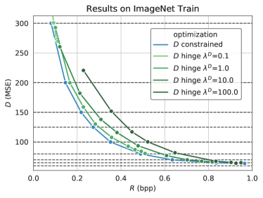
(a) $R$/$D$ performance for constrained optimization and hinge loss baselines. Dashed lines indicate the distortion target value $c_{D}$.

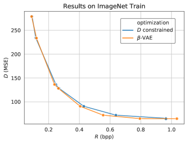
(b) $R$/$D$ performance for constrained optimization and $\beta$-VAE.

Figure 1: Training rate / distortion performance for the same model trained using different optimization methods.

1 Introduction

Deep latent variable models have started to outperform conventional baselines on lossy compression of images [4, 7, 25, 14, 15, 24, 23, 33, 36], video [19, 8, 21, 31, 37, 20, 27, 6, 12], and audio [39, 36]. Nearly all of these methods use a loss function of the form $D+\beta R$, where $D$ measures distortion, $R$ measures bitrate, and $\beta$ is a fixed tradeoff parameter. We refer to this approach as $\beta$-VAE [13], because this loss can be motivated from a variational perspective [12].

Despite its popularity, $\beta$-VAE has several drawbacks. Firstly, setting $\beta$ to target a specific point in the $R$/$D$ plane can be tricky. One can show that a model trained with a given $\beta$ should end up at that point on the $R$/$D$ curve where the slope $\frac{\partial R}{\partial D}$ equals $\beta$ [1]. However, because the shape of the $R$/$D$ curve depends on the model and hyperparameters, and because the $R$/$D$ curve can be very steep or flat in the low or high bitrate regime, choosing $\beta$ can be difficult.

Secondly, in order to compare models it is not sufficient to train one instance of each model because the converged models would likely differ in both rate and distortion, which yields inconclusive results unless one model dominates the other on both metrics. Instead, to compare models we need to train both at several $\beta$ values to generate $R$/$D$ curves that can be compared, which is computationally costly and slows down the research iteration cycle.

A more natural way to target different regions of the $R$/$D$ plane is to set a distortion constraint and find our model parameters through constrained optimization:

$$\min_{\boldsymbol{\theta}}R(\boldsymbol{\theta})\text{ s.t. }D(\boldsymbol{\theta})\leq c_{D},$$ (1)

where $\boldsymbol{\theta}$ refers to the joint parameters of the encoder, decoder and prior, and $c_{D}$ is a distortion target.

We can control the rate-distortion tradeoff by setting the distortion target value $c_{D}$. Setting this value is more intuitive than setting $\beta$, as it is independent of the slope of the $R$/$D$ curve, and hence independent of model and hyperparameters.

As a result, we can easily compare two different models trained with the same distortion constraint; as we have fixed the $D$ axis we only have to look at the $R$ performance for each model.

Note that one could also minimize the distortion subject to a rate constraint. This is less straightforward as putting too much emphasis on the rate loss at the beginning of training can lead to posterior collapse [3, 11, 40, 28, 32].

There is a large literature on constrained optimization, but most of it does not consider stochastic optimization and is limited to convex loss functions. In this paper we evaluate, in addition to $\beta$-VAE, two constrained optimization methods that are compatible with stochastic gradient descent training of deep networks: A simple method based on the hinge loss (free bits [17, 5, 1] but applied to distortion rather than rate), and the Lagrangian distortion-constrained optimization method of [29] ($D$-CO).

We evaluate these methods on a modern image compression system applied to a realistic compression benchmark. We report on suitable hyperparameters and practical considerations that are relevant in this domain. We show that $D$-CO outperforms the hinge method, and reaches a similar performance to $\beta$-VAE. At the same time, $D$-CO is easier to work with and allows for pointwise model selection.

2 Related Work

2.1 Constrained Optimization

Several works have proposed algorithms to train deep networks under equality or inequality constraints [22, 10, 9, 29]. We deploy the algorithm of [29] as the VAE context is most similar to our setup.

The focus of [29] is on generative modelling rather than data compression, and there are a number of reasons why the models trained in [29] are not directly applicable to data compression. Firstly, their models contain a stochastic encoder which is not suitable for lossy compression, where bits-back coding is inapplicable. Secondly, [29] do not report $R$/$D$ performance but instead report log-likelihood. Furthermore, their latent space is continuous while most compression papers use a discrete latent space that allows for entropy coding of the latents under the prior. Lastly, they use a fixed Guassian prior whereas in lossy compression powerful learnable priors are used to decrease the bitrate as much as possible. In this paper we focus on the implementation and evaluation of constrained optimization for practical lossy image compression.

2.2 Hinge Loss

Another approach that was proposed for constrained optimization (in the context of avoiding posterior collapse) is free-bits, where the rate loss is hinged $D+\beta\max(R-c_{R},0)$ [17, 5, 1]. Like constrained optimization, this loss allows us to set a target value, and as such has been used in lossy compression [23]. However, we find that this method is inferior to constrained optimization in terms of $R$/$D$ performance and has difficulty converging to the target value.

2.3 Variable Bitrate Models

A different approach of dealing with the rate-distortion tradeoff is to train a single model that can compress at different bitrates [34, 30, 7, 38]. However, some of these works do not meet the performance achieved with specialized models [38] or require disjoint training of autoencoder and prior [34]. Other methods could benefit from constrained optimization (e.g. [38] still uses $\beta$ multipliers that could be replaced by a distortion target), an exercise that is left for future research.

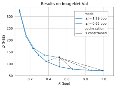
(a) $D$-CO: $\min_{\boldsymbol{\theta}}R(\boldsymbol{\theta})$ s.t. $D(\boldsymbol{\theta})\leq c_{d}$

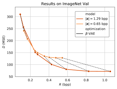
(b) $\beta$-VAE: $\min_{\boldsymbol{\theta}}D(\boldsymbol{\theta})+\beta R(\boldsymbol{\theta})$

Figure 2: Model selection using (a) distortion constrained optimization and (b) $\beta$-VAE. The baseline model (dark line) is altered by halving the number of latent channels (light line). Models that are trained using the same distortion target (a) or the same value of $\beta$ (b) are connected using a dotted line.

3 Method

3.1 Constrained Optimization

The Lagrangian of the primal problem in equation 1 is:

$$\mathcal{L}_{\text{Lagrangian}}(\boldsymbol{\theta},\lambda^{D})=R(\boldsymbol{\theta})+\lambda^{D}\left(D(\boldsymbol{\theta})-c_{D}\right)$$ (2)

For a convex problem, we would find the minimum of the dual at $\max_{\lambda^{D}}\min_{\boldsymbol{\theta}}\mathcal{L}_{\text{Lagrangian}}(\boldsymbol{\theta},\lambda^{D})$.

For non-convex deep learning models, we deploy the algorithm proposed by [29] and iteratively update $\boldsymbol{\theta}$ and $\lambda^{D}$ using stochastic gradient descent and ascent respectively.

Note that the $\beta$-VAE loss is the Lagrangian of a rate-constrained optimization. However, the multiplier $\lambda^{R}=\beta$ is either fixed or updated according to a heuristic schedule [3, 11, 40, 28, 32], and thus no constrained optimization is performed.

Because we found that the optimal $D$-CO hyperparameters were different depending on the target value, we normalize our constraint function by the target value. Our loss function thus becomes:

$$\mathcal{L}_{D-\text{CO}}(\boldsymbol{\theta},\lambda^{D})=R(\boldsymbol{\theta})+\lambda^{D}\left(\dfrac{D(\boldsymbol{\theta})}{c_{D}}-1\right)$$ (3)

3.1.1 Weight and Multiplier Updates

For each minibatch, we update $\boldsymbol{\theta}$ using the Adam optimizer, and $\lambda^{D}$ using SGD with momentum, to respectively minimize and maximize the batchwise Lagrangian (Eq. 3).

Like [29], we reparametrize $\mu^{D}=\log\lambda^{D}$ in order to enforce the positivity of $\lambda^{D}$ (to satisfy the K.K.T. [18, 16] conditions for inequality constraints). We also follow them in updating $\Delta\mu^{D}_{t+1}\propto\frac{\partial\mathcal{L}}{\partial\lambda^{D}_{t}}=\frac{D_{t}}{c_{D}}-1$ as this resulted in smoother updates of our multipliers than using the actual gradient $(\frac{D_{t}}{c_{D}}-1)\exp{(\mu^{D}_{t})}$.

We use a high momentum ($\alpha=0.99$) for our multiplier updates, to ensure a smooth multiplier trajectory despite the high variance of the MSE loss. As we use the PyTorch [26] SGD implementation, we make sure to set dampening to be equal to momentum. We clip our log-multiplier s.t. $\lambda^{D}\leq 10^{3}$ for stability.

Unlike [29] we choose to set our initial value of $\lambda^{D}$ to the clip value $\lambda^{D}_{0}=10^{3}$. This way, we focus on training the autoencoder for distortion at the beginning of training, which we found to be essential for high performance. The final multiplier trajectories are shown in Figure 3.

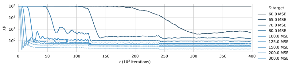
Figure 3: Trajectory of Lagrangian multipliers during training. Each curve represents a model with a different constraint.

4 Experiments

We conduct a series of experiments to show how constrained optimization is more suitable for training lossy compression models than $\beta$-VAE or distortion hinge baselines.

4.1 General Setup

We use the autoencoder architecture of [23] but without the mask. Our prior is the gated pixelCNN [35] as used in [12]. Like [12] we jointly train our code-model and autoencoder, without any detaching of the gradients. We use scalar quantization with a learned codebook and a straight-trough estimator (hardmax during forward pass and softmax gradient during backward) [2, 23, 12].

We train our model on random 160x160 crops of ImageNet Train, and evaluate on 160x160 center crops of ImageNet Validation. Like [23] we resize the smallest side of all images to 256 to reduce compression artifacts.

We train using the rate loss expressed in bits per pixel (bpp) and using the distortion loss expressed in average MSE computed on unnormalized images on a 0-255 scale.

We update our parameters using Adam with a learning rate of $2\cdot 10^{-3}$ for the autoencoder and $1\cdot 10^{-4}$ for the prior. We decay both learning rates every 3 epochs (120087 iterations) by a factor of $0.1$. For the multiplier updates, we use SGD with a learning rate of $5\cdot 10^{-3}$. We use a batch size of 32.

4.2 $D$-CO vs. $D$-hinge

For this experiment we choose exponentially spaced $D$-constraint values (60, 65, 70, 80, 100, 125, 150, 200, 300 MSE) and look at how well the methods converge to the set target. We compare our $D$-CO training with the simpler $D$-hinge baselines of the form:

$$\mathcal{L}_{D\text{-hinge}}(\boldsymbol{\theta})=R(\boldsymbol{\theta})+\lambda^{D}\max\left(\dfrac{D(\boldsymbol{\theta})}{c_{D}}-1,0\right)$$ (4)

Unlike $D$-CO, $\lambda^{D}$ is fixed during training, but we train models with different values (0.01, 0.1, 1, 10, 100). In line with $D$-CO, we use the normalized constraint function as we verified that it worked better than the unnormalized one.

Results are shown in Figure 1a. Observe that the $D$-CO models converge very closely to the set target (within 1 MSE point for achievable constraints). For the hinge models, the constraint is not satisfied reliably and overall $R$/$D$ performance is worse (some models converged to $R$/$D$ values outside of the chosen display range). Furthermore, the hinge models are sensitive to the value of $\lambda_{D}$, and the optimal value differs per target.

Figure 3 shows the trajectories of the $D$-CO multipliers. For stricter constraints, it takes longer before the multiplier starts to drop, changing emphasis from $D$ to $R$. In the limit of an unachievable constraint (MSE $<62$), the multiplier remains constant at the clip value. All multipliers converge to a relatively stable final value, which is dependent on the target (as expected since the $\frac{\partial R}{\partial D}$ slope is different).

4.3 $D$-CO vs. $\beta$-VAE

In the next experiment, we compare the $R$/$D$ performance of $D$-CO to the $\beta$-VAE baseline. We first train $\beta$-VAE models for exponentially spaced $\beta$ values (0.1, 10, 50, 100, 200, 250, 500, 750). For each $\beta$-VAE, we use the distortion loss over the last training epoch as the target for training a $D$-CO model.

Results are shown in Figure 1b (PSNR results in Figure A.1). The $R$/$D$ performance of the $D$-CO models is similar to that of the $\beta$-VAEs. For bitrates higher than 0.4 bpp, we see a slight advantage for the $\beta$-VAE. For these target values, the $D$-CO multipliers are almost constant (see the strict constraints in Figure 3) and we thus attribute this difference to the optimization hyperparameters being fine-tuned for the scale of the $\beta$-VAE loss.

4.4 Model Selection

In the final experiment we highlight how constrained optimization can simplify the model selection process. We adapt our architecture by changing the number of latent channels from $32$ to $16$, effectively halving the maximum channel capacity from 1.29 bpp to 0.64 bpp. We train $\beta$-VAE models for the $\beta$s from Section 4.3 and $D$-CO models using the targets from Section 4.2.

Results are shown in Figure 2. For both optimization methods, the lowest achievable distortion has increased from $\sim 70$ MSE to $\sim 130$ MSE for the model with decreased channel capacity.

For the $\beta$-VAE optimization, points with the same $\beta$ now end up at very different points on the $R$/$D$ plane. For the half-capacity model, we cover a narrow range of 240-128 MSE.

In contrast, $D$-CO produces two comparable $R$/$D$ curves. Distortion targets below 130 MSE are unachievable for the half-capacity model and are all collapsed into a single point. However, for any achievable distortion target, both models end up with a similar distortion which allows us to do a pointwise comparison.

5 Conclusion

We present distortion constrained optimization ($D$-CO) as an alternative to $\beta$-VAE training for lossy compression. We report suitable hyperparameters and propose to normalize the constraint function for better performance. We demonstrate that $D$-CO gives similar performance to $\beta$-VAE on a realistic image compression task, while at the same time providing a more intuitive way to balance the rate and distortion losses. Finally, we show how $D$-CO can facilitate the model selection process by allowing pointwise model comparisons.

Appendix A Supplementary Material

A.1 PSNR Results

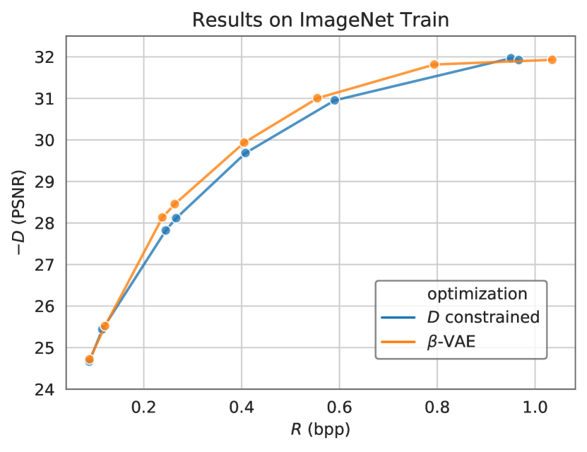
Figure A.1: Rate / PSNR performance for $D$ constrained optimization and $\beta$-VAE.

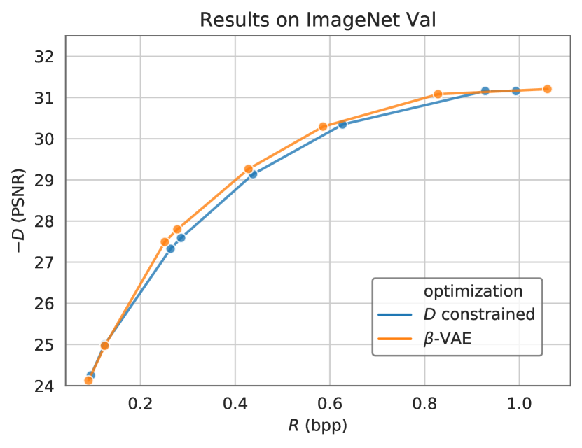
Figure A.2: Validation Rate / PSNR performance for $D$ constrained optimization and $\beta$-VAE.

References

- [1] Alexander A Alemi, Ben Poole, Ian Fischer, Joshua V Dillon, Rif A Saurous, and Kevin Murphy. Fixing a broken ELBO, 2018. In International Conference on Machine Learning, 2018.
- [2] Yoshua Bengio, Nicholas Léonard, and Aaron C. Courville. Estimating or propagating gradients through stochastic neurons for conditional computation. CoRR, abs/1308.3432, 2013.
- [3] Samuel R. Bowman, Luke Vilnis, Oriol Vinyals, Andrew Dai, Rafal Jozefowicz, and Samy Bengio. Generating sentences from a continuous space. In Proceedings of The 20th SIGNLL Conference on Computational Natural Language Learning, pages 10–21, Berlin, Germany, Aug. 2016. Association for Computational Linguistics.
- [4] C Cai, L Chen, X Zhang, G Lu, and Z Gao. A novel deep progressive image compression framework. In 2019 Picture Coding Symposium (PCS), pages 1–5, Nov. 2019.
- [5] Xi Chen, Diederik P. Kingma, Tim Salimans, Yan Duan, Prafulla Dhariwal, John Schulman, Ilya Sutskever, and Pieter Abbeel. Variational lossy autoencoder. In 5th International Conference on Learning Representations, ICLR 2017, Toulon, France, April 24-26, 2017, Conference Track Proceedings. OpenReview.net, 2017.
- [6] Z. Chen, T. He, X. Jin, and F. Wu. Learning for video compression. IEEE Transactions on Circuits and Systems for Video Technology, 30(2):566–576, 2020.
- [7] Yoojin Choi, Mostafa El-Khamy, and Jungwon Lee. Variable rate deep image compression with a conditional autoencoder. In Proceedings of the IEEE International Conference on Computer Vision, pages 3146–3154, 2019.
- [8] Abdelaziz Djelouah, Joaquim Campos, Simone Schaub-Meyer, and Christopher Schroers. Neural Inter-Frame compression for video coding. In Proceedings of the IEEE International Conference on Computer Vision, pages 6421–6429, 2019.
- [9] R Fletcher. Practical Methods of Optimization. John Wiley & Sons, June 2013.
- [10] Pascal Fua, Aydin Varol, Raquel Urtasun, and Mathieu Salzmann. Least-squares minimization under constraints. Technical report, EPFL, 2010.
- [11] Ishaan Gulrajani, Kundan Kumar, Faruk Ahmed, Adrien Ali Taiga, Francesco Visin, David Vazquez, and Aaron Courville. Pixelvae: A latent variable model for natural images. In 5th International Conference on Learning Representations, 2017.
- [12] Amirhossein Habibian, Ties van Rozendaal, Jakub M Tomczak, and Taco S Cohen. Video compression with rate-distortion autoencoders. In Proceedings of the IEEE International Conference on Computer Vision, pages 7033–7042. openaccess.thecvf.com, 2019.
- [13] Irina Higgins, Loic Matthey, Arka Pal, P. Christopher Burgess, Xavier Glorot, Matthew Botvinick, Shakir Mohamed, and Alexander Lerchner. beta-vae: Learning basic visual concepts with a constrained variational framework. International Conference on Learning Representations, 2017.
- [14] Nick Johnston, Elad Eban, Ariel Gordon, and Johannes Ballé. Computationally efficient neural image compression. CoRR, abs/1912.08771, 2019.
- [15] Nick Johnston, Damien Vincent, David Minnen, Michele Covell, Saurabh Singh, Troy Chinen, Sung Jin Hwang, Joel Shor, and George Toderici. Improved lossy image compression with priming and spatially adaptive bit rates for recurrent networks. In Proceedings of the IEEE Conference on Computer Vision and Pattern Recognition, pages 4385–4393, 2018.
- [16] William Karush. Minima of functions of several variables with inequalities as side constraints. M. Sc. Dissertation. Dept. of Mathematics, Univ. of Chicago, 1939.
- [17] Durk P Kingma, Tim Salimans, Rafal Jozefowicz, Xi Chen, Ilya Sutskever, and Max Welling. Improved variational inference with inverse autoregressive flow. In D D Lee, M Sugiyama, U V Luxburg, I Guyon, and R Garnett, editors, Advances in Neural Information Processing Systems 29, pages 4743–4751. Curran Associates, Inc., 2016.
- [18] Harold W Kuhn and Albert W Tucker. Nonlinear programming. In Traces and emergence of nonlinear programming, pages 247–258. Springer, 2014.
- [19] Haojie Liu, Han Shen, Lichao Huang, Ming Lu, Tong Chen, and Zhan Ma. Learned video compression via joint Spatial-Temporal correlation exploration. CoRR, abs/1912.06348, Dec. 2019.
- [20] Salvator Lombardo, Jun Han, Christopher Schroers, and Stephan Mandt. Deep generative video compression. In Advances in Neural Information Processing Systems 32, pages 9287–9298. Curran Associates, Inc., 2019.
- [21] Guo Lu, Wanli Ouyang, Dong Xu, Xiaoyun Zhang, Chunlei Cai, and Zhiyong Gao. Dvc: An end-to-end deep video compression framework. In The IEEE Conference on Computer Vision and Pattern Recognition (CVPR), June 2019.
- [22] Pablo Márquez-Neila, Mathieu Salzmann, and Pascal Fua. Imposing hard constraints on deep networks: Promises and limitations. CoRR, abs/1706.02025, June 2017.
- [23] Fabian Mentzer, Eirikur Agustsson, Michael Tschannen, Radu Timofte, and Luc Van Gool. Conditional Probability Models for Deep Image Compression. In Proceedings of the IEEE Conference on Computer Vision and Pattern Recognition, pages 4394–4402, Jan. 2018.
- [24] David Minnen, Johannes Ballé, and George D Toderici. Joint autoregressive and hierarchical priors for learned image compression. In S. Bengio, H. Wallach, H. Larochelle, K. Grauman, N. Cesa-Bianchi, and R. Garnett, editors, Advances in Neural Information Processing Systems 31, pages 10771–10780. Curran Associates, Inc., 2018.
- [25] David Minnen and Saurabh Singh. Channel-wise autoregressive entropy models for learned image compression, 2020.
- [26] Adam Paszke, Sam Gross, Francisco Massa, Adam Lerer, James Bradbury, Gregory Chanan, Trevor Killeen, Zeming Lin, Natalia Gimelshein, Luca Antiga, Alban Desmaison, Andreas Kopf, Edward Yang, Zachary DeVito, Martin Raison, Alykhan Tejani, Sasank Chilamkurthy, Benoit Steiner, Lu Fang, Junjie Bai, and Soumith Chintala. Pytorch: An imperative style, high-performance deep learning library. In Advances in Neural Information Processing Systems 32, pages 8024–8035. Curran Associates, Inc., 2019.
- [27] Jorge Pessoa, Helena Aidos, Pedro Tomás, and Mário AT Figueiredo. End-to-end learning of video compression using spatio-temporal autoencoders, 2018.
- [28] Tapani Raiko, Harri Valpola, Markus Harva, and Juha Karhunen. Building blocks for variational bayesian learning of latent variable models. J. Mach. Learn. Res., 8(Jan):155–201, 2007.
- [29] Danilo J Rezende and Fabio Viola. Generalized ELBO with constrained optimization, GECO. In Workshop on Bayesian Deep Learning, NeurIPS. pdfs.semanticscholar.org, 2018.
- [30] Oren Rippel and Lubomir Bourdev. Real-time adaptive image compression. In Proceedings of the 34th International Conference on Machine Learning-Volume 70, pages 2922–2930. JMLR. org, 2017.
- [31] Oren Rippel, Sanjay Nair, Carissa Lew, Steve Branson, Alexander G Anderson, and Lubomir Bourdev. Learned video compression. In Proceedings of the IEEE International Conference on Computer Vision, pages 3454–3463, 2019.
- [32] Casper Kaae Sønderby, Tapani Raiko, Lars Maaløe, SøRen Kaae Sønderby, and Ole Winther. Ladder variational autoencoders. In D D Lee, M Sugiyama, U V Luxburg, I Guyon, and R Garnett, editors, Advances in Neural Information Processing Systems 29, pages 3738–3746. Curran Associates, Inc., 2016.
- [33] L. Theis, W. Shi, A. Cunningham, and F. Huszár. Lossy image compression with compressive autoencoders. In International Conference on Learning Representations, 2017.
- [34] George Toderici, Sean M O’Malley, Sung Jin Hwang, Damien Vincent, David Minnen, Shumeet Baluja, Michele Covell, and Rahul Sukthankar. Variable Rate Image Compression with Recurrent Neural Networks. CoRR, abs/1511.06085, Nov. 2015.
- [35] Aaron van den Oord, Nal Kalchbrenner, Lasse Espeholt, Koray Kavukcuoglu, Oriol Vinyals, and Alex Graves. Conditional Image Generation with PixelCNN Decoders. In D D Lee, M Sugiyama, U V Luxburg, I Guyon, and R Garnett, editors, Advances in Neural Information Processing Systems 29, pages 4790–4798. Curran Associates, Inc., 2016.
- [36] Aaron van den Oord, Oriol Vinyals, et al. Neural discrete representation learning. In Advances in Neural Information Processing Systems, pages 6306–6315, 2017.
- [37] Chao-Yuan Wu, Nayan Singhal, and Philipp Krahenbuhl. Video compression through image interpolation. In Proceedings of the European Conference on Computer Vision (ECCV), pages 416–431, 2018.
- [38] Yibo Yang, Robert Bamler, and Stephan Mandt. Variable-bitrate neural compression via bayesian arithmetic coding. CoRR, abs/2002.08158, 2020.
- [39] Yang Yang, Guillaume Sautière, J Jon Ryu, and Taco S Cohen. Feedback Recurrent AutoEncoder. 2020 IEEE International Conference on Acoustics, Speech and Signal Processing (ICASSP), Nov. 2019.
- [40] Zichao Yang, Zhiting Hu, Ruslan Salakhutdinov, and Taylor Berg-Kirkpatrick. Improved variational autoencoders for text modeling using dilated convolutions. In Proceedings of the 34th International Conference on Machine Learning-Volume 70, pages 3881–3890. JMLR. org, 2017.