[Preprint]
An Extensive Study on Cross-Dataset Bias and Evaluation Metrics Interpretation for Machine Learning applied to Gastrointestinal Tract Abnormality Classification

Abstract.

Precise and efficient automated identification of Gastrointestinal (GI) tract diseases can help doctors treat more patients and improve the rate of disease detection and identification. Currently, automatic analysis of diseases in the GI tract is a hot topic in both computer science and medical-related journals. Nevertheless, the evaluation of such an automatic analysis is often incomplete or simply wrong. Algorithms are often only tested on small and biased datasets, and cross-dataset evaluations are rarely performed. A clear understanding of evaluation metrics and machine learning models with cross datasets is crucial to bring research in the field to a new quality level. Towards this goal, we present comprehensive evaluations of five distinct machine learning models using Global Features and Deep Neural Networks that can classify 16 different key types of GI tract conditions, including pathological findings, anatomical landmarks, polyp removal conditions, and normal findings from images captured by common GI tract examination instruments. In our evaluation, we introduce performance hexagons using six performance metrics such as recall, precision, specificity, accuracy, F1-score, and Matthews Correlation Coefficient to demonstrate how to determine the real capabilities of models rather than evaluating them shallowly. Furthermore, we perform cross-dataset evaluations using different datasets for training and testing. With these cross-dataset evaluations, we demonstrate the challenge of actually building a generalizable model that could be used across different hospitals. Our experiments clearly show that more sophisticated performance metrics and evaluation methods need to be applied to get reliable models rather than depending on evaluations of the splits of the same dataset, i.e., the performance metrics should always be interpreted together rather than relying on a single metric.

1. Introduction

Cancer is one of the leading causes of death worldwide and a significant barrier to life expectancy (Bray et al., 2018). In particular, the Gastrointestinal (GI) tract can be affected by a variety of diseases and abnormalities (Pogorelov et al., 2017d). Using data from the Global Cancer Observatory, Bray et al. (2018) estimated that, for 2018, there would be around 5 million new luminal GI cancer incidences and about 3.6 million deaths due to GI cancer. The most frequently diagnosed GI cancers in 2018 for new cases are Colorectal Cancer (CRC) (6.1%), stomach cancer (5.7%), liver cancer (4.7%), rectum cancer (3.9%), and esophageal cancer (3.2%) out of 36 types of cancers (Bray et al., 2018).

Gastroscopy and colonoscopy are the most successful medical procedures for GI endoscopy examinations. Among both, colonoscopy has been proven to be an effective preventative method by improving declination in the occurrence of CRC by 30% (Lieberman, 2005). During a colonoscopic procedure, endoscopists insert a colonoscope carefully through the anus to examine the rectum and colon. A tiny wide-angle video camera mounted at the end of the colonoscope captures a live video signal of the internal mucosa of the patient’s colon. The endoscopist uses the video signal for real-time diagnosis of the patient, where one of the primary goals is to identify and remove abnormalities such as polyps (Wang et al., 2015).

The current EU guidelines (Von Karsa et al., 2012) recommend GI tract screening for all people above 50 years. Such regular screenings can be of great significance for early detection and prevention of cancer inside the GI tract, but they are challenging due to many factors. Moreover, a colonoscopy examination is entirely an operator-dependent screening procedure (Shin and Balasingham, 2017). The detection rate of GI tract lesions mostly relies on the clinical experience of the gastroenterologist. The shortage of experienced gastroenterologists, and the clinicians’ tiredness and lack of concentration during the colonoscopic examination, can lead to missing polyps that otherwise would be detected (Tajbakhsh et al., 2016a). The estimated miss rate for the subject undergoing a colonoscopy examination is 25% (Leufkens et al., 2012).

Although considerable work has been done to develop and improve systems for automatic polyp detection, the performance of existing solutions are still behind that of an expert endoscopist (de Lange et al., 2018; Mori and Kudo, 2018; Wang et al., 2018; Wang et al., 2014; Bernal et al., 2012). Most of the published papers in the field use non-public datasets or develop models from too small training, validation, and test sets (Wang et al., 2014; Bernal et al., 2012; Wang et al., 2018). The performance metrics used to measure the performance of methods are also not sufficient (for example, see the first part of Table 1). Thus, it is difficult for researchers to compare and reproduce some of the present related works. Moreover, the state of the art research in this field does not present the generalizability of their solutions using cross-dataset evaluations. As a result, it makes a distrust for applying these machine learning (ML) solutions in practice.

An automatic and efficient Computer-Aided Diagnosis (CAD) system in a clinic could assist medical experts during the endoscopic and colonoscopy procedure to improve the detection rate by finding unrecognized lesions and act as a second observer by providing better insights to the gastroenterologist concerning the presence and types of lesions. With this inspiration, we conducted five experiments to classify $16$ classes of GI tract conditions for the Medico Multimedia Task at MediaEval 2018 (Pogorelov et al., 2018b). One example for each of the 16 classes is depicted in Figure 1.

In this work, we focus on identifying the limitations of generalizing ML models across different datasets and how to interpret the evaluation metrics in that context. For this, we are using Global Feature (GF)-based and deep learning (DL)-based methods that performed well at the 2018 Medico Task (Pogorelov et al., 2018b) where one specific dataset was used. In addition, we here explore the different performance metrics of both methods (GF and DL) to identifying the limitations of each. We show that combined complex Deep Neural Network (DNN) models outperform other methods. Finally, we explore how multiclass models perform on polyp and non-polyps detection with and without retraining the model for the two specific classes. The effects of retraining for classifying the sub-categories of the same dataset and using them in other datasets are analyzed in detail to identify the cross-dataset generalization capabilities of our models. We emphasize that a large number of performance measures do not show the real performance of ML models. We also highlight the necessity of having cross-dataset evaluations to determine the real capabilities of ML models before using them in clinical settings.

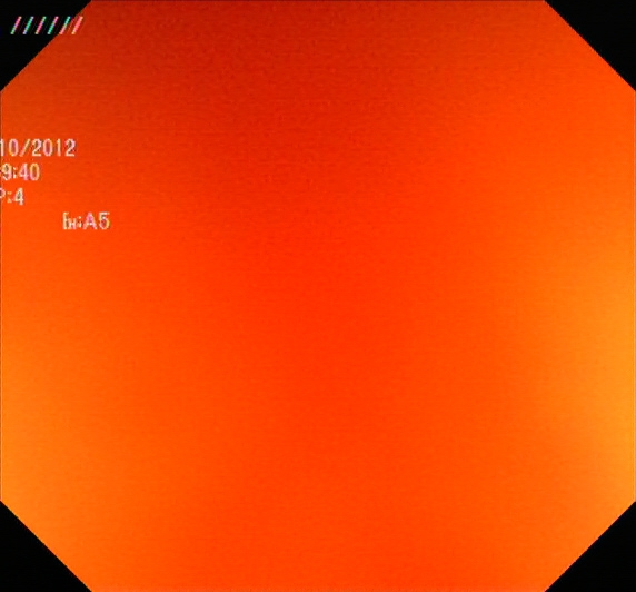
(a)

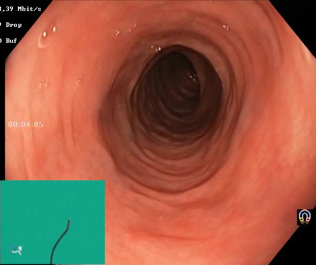
(b)

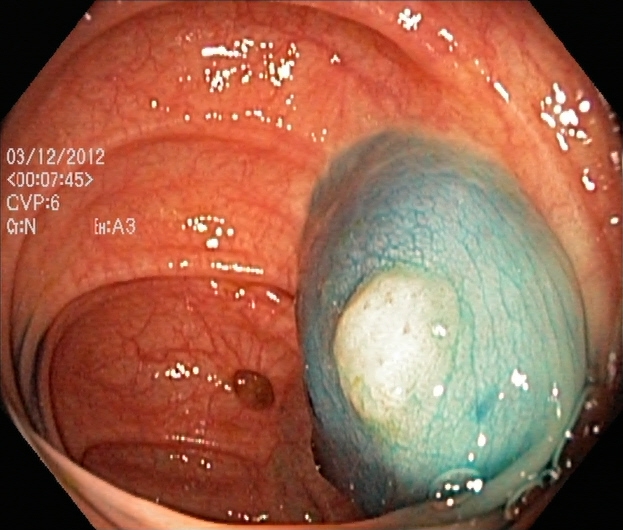
(c)

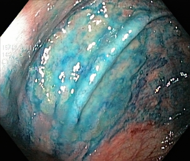
(d)

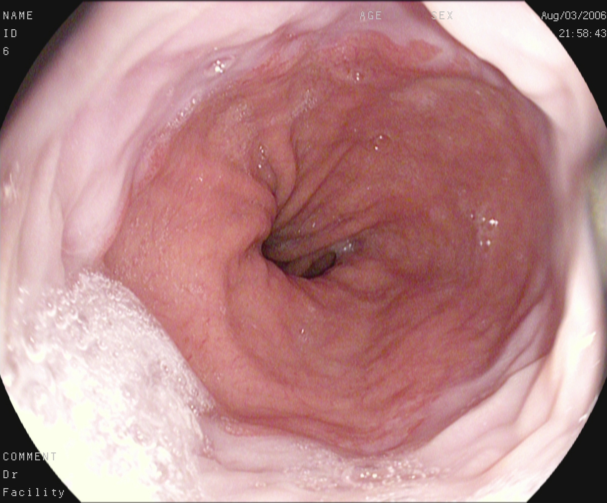
(e)

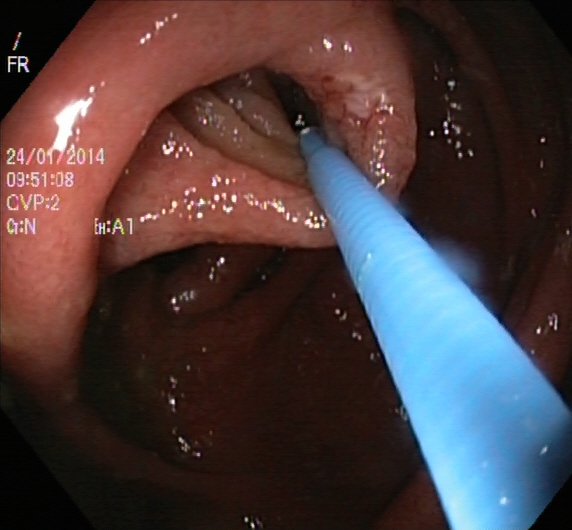
(f)

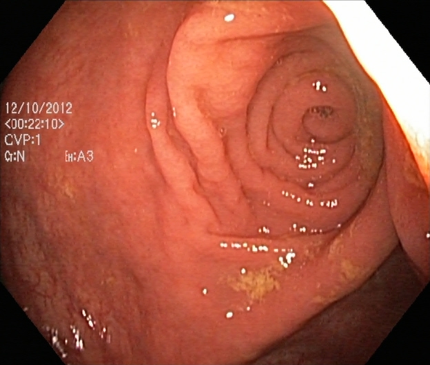
(g)

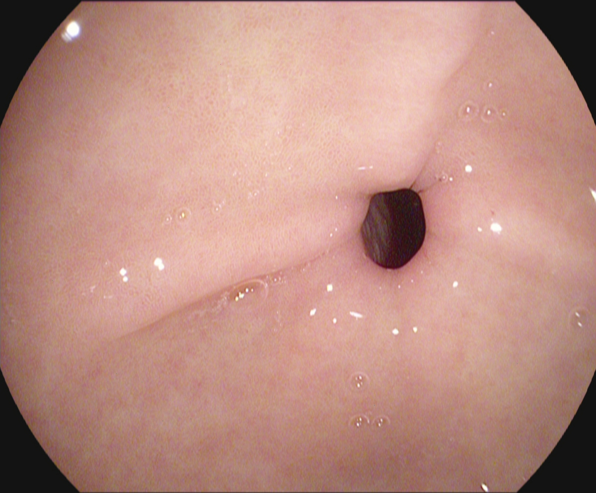
(h)

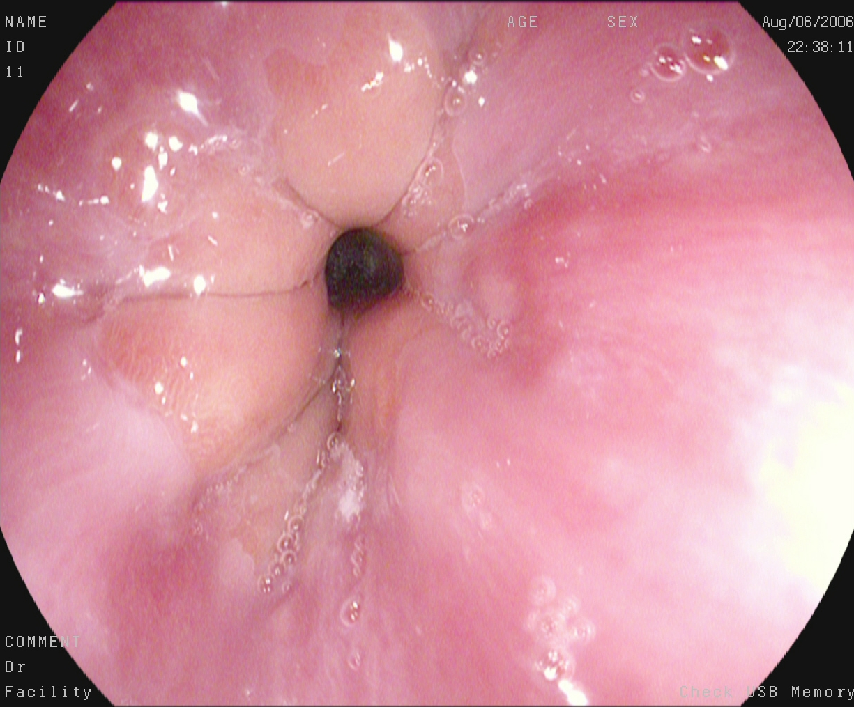
(i)

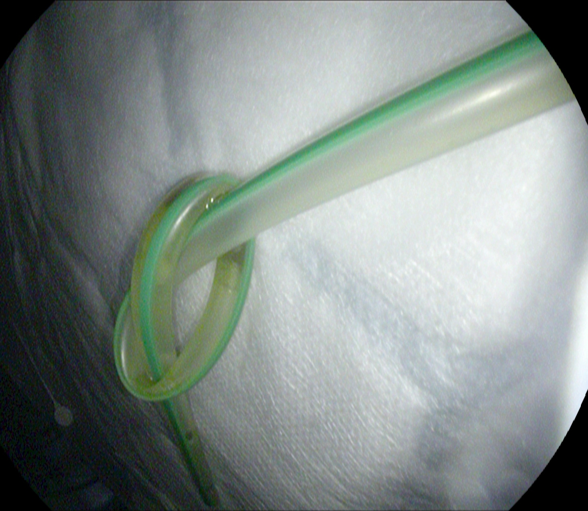
(j)

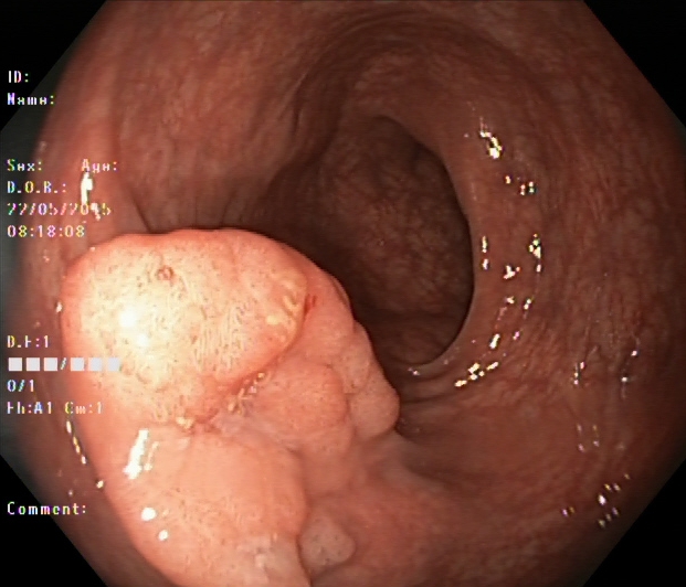
(k)

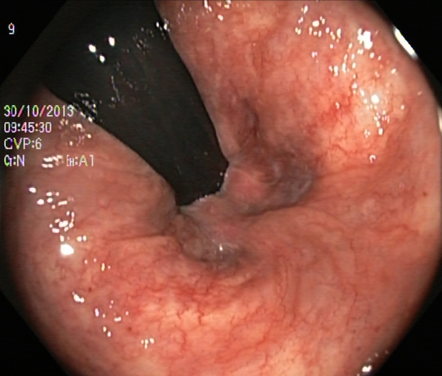
(l)

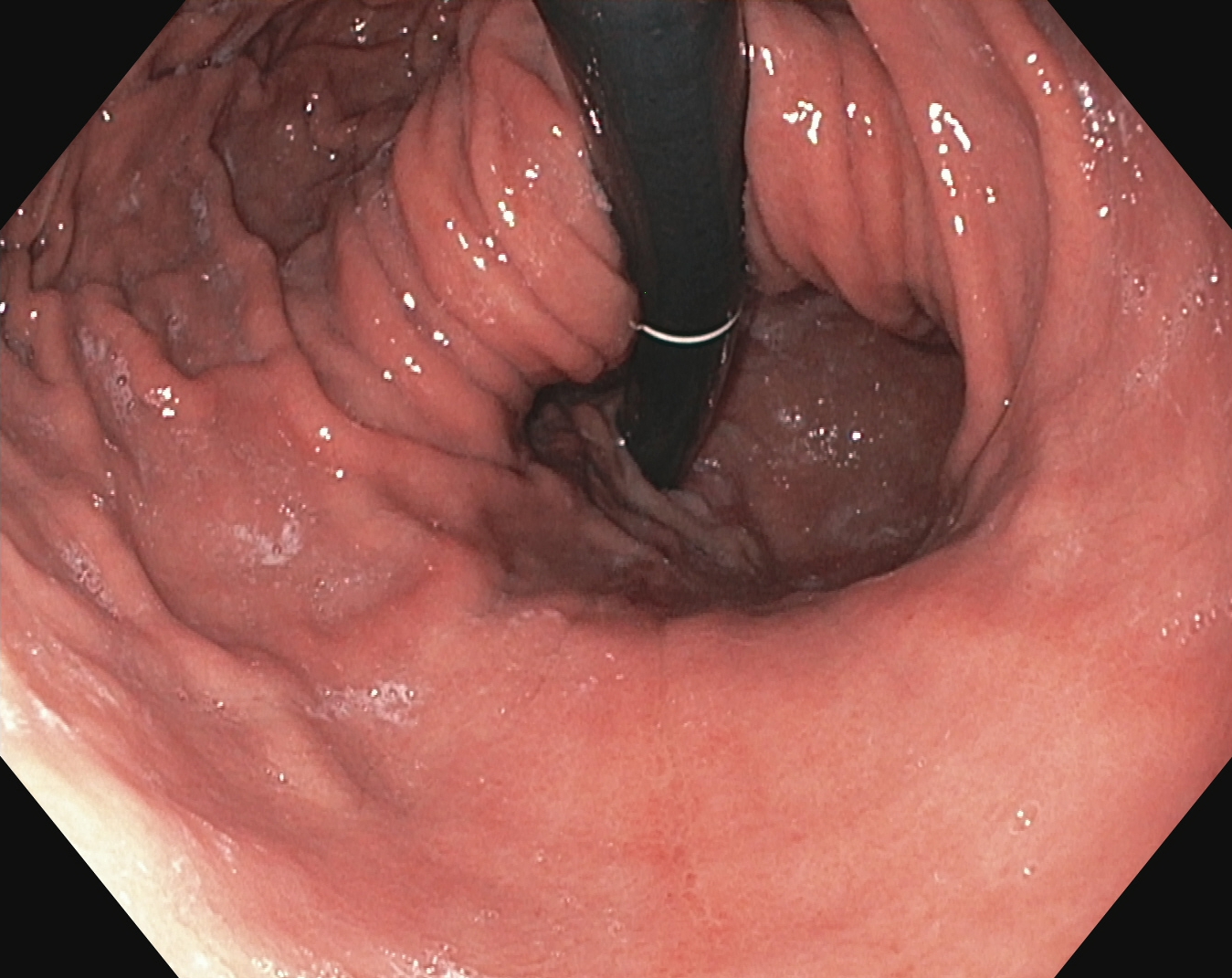
(m)

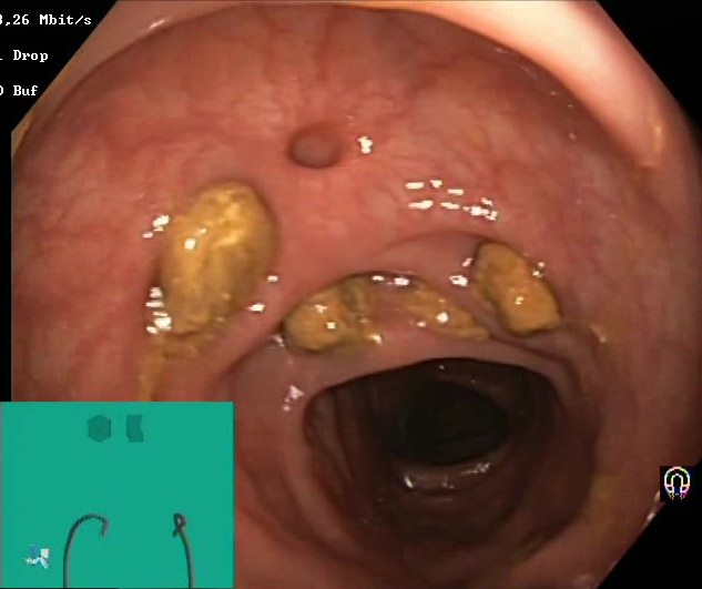
(n)

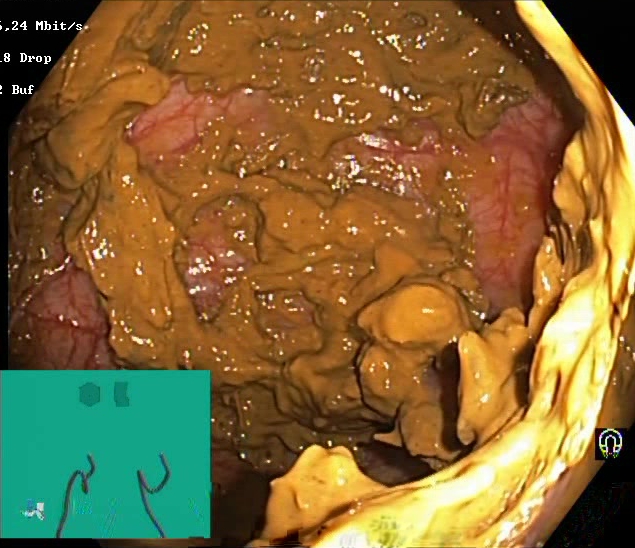
(o)

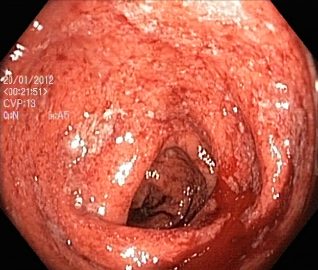
(p)

Figure 1. Sample images of GI findings. Each image represents one of the 16 classes from the dataset used for the Medico 2018 challenge (Pogorelov et al., 2017c, a).

In order to study cross-dataset bias and metrics interpretation, our contributions are as follows:

1. We present five ML classification models to classify multi-class findings (anatomical landmark, pathological findings, polyp removal conditions, and normal findings) of the GI tract. Using a limited imbalanced dataset, we experiment with approaches ranging from GF approaches to simple DNN and complex DNN approaches with transfer learning. Moreover, we present a detailed evaluation using six performance metrics to show the real classification performance of ML models. In addition, we analyze and present detailed evaluation results of using multi-class classification ML models for classifying binary classes (subclasses of the multi-class categories) with and without retraining to evaluate the generalizability of our models. We emphasize the difficulties of using well-performing ML methods in cross-datasets as a result of the reluctance of ML models to cross-dataset generalization. We present this negative impact with the aid of another evaluation using Receiver Operating Characteristic (ROC) and Precision-Recall Curve (PRC) curves of the best model. We also demonstrate when a ROC curve is good to use and when it is better to use a PRC curve.

2. With the above point, we emphasis the requirement of detailed cross-dataset evaluations to identify generalizability of ML models before using them as universal models in live applications. Because good performance measures with a single dataset do not necessarily imply good real-world performance, we argue that researchers should present cross-dataset evaluations for building generalizable model rather than presenting performance values for the test datasets, which is separated from the same training data source.

Moreover, with respect to the 2018 Medico Task (Pogorelov et al., 2018b), our best DNN method achieved the highest recall, specificity and accuracy for multi-class classification of the GI tract findings. We achieved an Matthews Correlation Coefficient (MCC) (0.0029 less) and an Rk correlation coefficient (0.0001 less) nearly equal to the winning team. With this achievement, we demonstrate all the steps from designing to training and testing for reaching such performance using this model and its expandability using different pre-trained networks.

In the next section, we present related work and the performance of relevant existing solutions. Section 3 discusses the methodology used for our GF-based approaches and the theoretical foundation for our work. The DNN-based approaches are similarly described in Section 4. Our experimental results are presented and analyzed in Section 5, followed by a discussion in Section 6 on how our results can be helpful for other researchers. Finally, in Section 7, we conclude our findings.

2. Related Work

Table 1. Overview of the related work. REC = Recall (Sensitivity), SPEC = Specificity, ACC = Accuracy, MCC = Matthews Correlation Coefficient, F1 = F1 Score, Rk = Rk correlation coefficient, FPS = Frame Per Second. The results of the Medico Task may slightly vary compared to the proceeding note papers because of different ways of calculating the multi-class performance metrics by the organizers.

Reference	Year	REC	PREC	SPEC	ACC	MCC	F1	Rk	FPS
Hwang et al. (Hwang et al., 2007)	2007	0.9600	0.8300	-	-	-	-	-	15
Li et al. (Li and Meng, 2012)	2012	0.8860	-	0.9620	0.9240	-	-	-	-
Zhou et al. (Zhou et al., 2014)	2014	0.7500	-	0.9592	0.9077	-	-	-	-
Wang et al.(Wang et al., 2014)	2014	0.8140	-	-	-	-	-	-	0.14
Mamonov et al. (Mamonov et al., 2014)	2014	0.4700	-	0.9000	-	-	-	-	-
Wang et al. (Wang et al., 2015)	2015	0.9770	-	-	0.9570	-	-	-	10
Riegler et al.(Riegler et al., 2016)	2016	0.9850	0.9388	0.7250	0.8770	-	-	-	$\sim$ 300
Shin et al. (Shin and Balasingham, 2017)	2017	0.9082	0.9271	0.9176	0.9126	-	-	-	-
Riegler et al. (Riegler et al., 2017a)	2017	0.9850	0.9390	0.7250	0.8770	-	-	-	$\sim$ 75
Yu et al. (Yu et al., 2017)	2017	0.5005	0.4917	-	0.9471	-	0.4830	0.5357	-
Pogorelov et al. (Pogorelov et al., 2017e)	2017	0.8260	0.8290	0.9750	0.9570	-	0.8260	0.8020	46
Agrawal et al. (Agrawal et al., 2017)	2017	-	-	-	0.9610	0.8260	0.8470	-	-
Naqvi et al. (Naqvi et al., 2017)	2017	-	0.7665	0.9660	0.9420	0.7360	0.7670	-	-
Petscharnig et al. (Petscharnig et al., 2017)	2017	0.7550	0.7550	0.9650	0.9390	0.7200	0.7550	0.7240	-
Pogorelov et al. (Pogorelov et al., 2017d)	2017	0.9060	0.9060	0.9810	0.9690	-	-	-	30
Yuan et al. (Yuan et al., 2018)	2018	0.8180	0.7232	-	-	-	0.7431	-	-
Wang et al. (Wang et al., 2018)	2018	0.9438	-	0.9592		-	-	-	-
Mori et al. (Mori and Kudo, 2018)	2018	¿0.9000	-	¿0.9000	-	-	-	-	-
MediaEval 2018 Medico Task (Pogorelov et al., 2018b)    [ All the experiments below are done using 2018 Medico dataset]
Hoang et al. (Hoang et al., 2018)	2018	0.9281	0.9426	0.9963	0.9932	0.9312	0.9342	0.9398	23
Hicks et al. (Hicks et al., 2018)	2018	0.9218	0.9378	0.9959	0.9924	0.9228	0.9236	0.9325	624
Borgli et al. (Borgli et al., 2018)	2018	0.8572	0.8708	0.9956	0.9918	0.8555	0.8555	0.9280	-
Kirkerød et al. (Kirkerød et al., 2018)	2018	0.8433	0.8514	0.9944	0.9896	0.8366	0.8367	0.9082	-
Dias et al. (Dias and Dias, 2018)	2018	0.8205	0.8414	0.9938	0.9885	0.8146	0.8114	0.8983	8.61
Taschwer et al. (Taschwer et al., 2018)	2018	0.8673	0.8826	0.9933	0.9876	0.8641	0.8662	0.8897	-
Ostroukhova et al. (Ostroukhova et al., 2018)	2018	0.8236	0.8281	0.9911	0.9835	0.8115	0.8145	0.8539	1E-100
Khan et al. (Khan and Tahir, 2018)	2018	0.6203	0.7173	0.9767	0.957	0.6025	0.5868	0.6302	43329
Steiner et al. (Steiner et al., 2018)	2018	0.4219	0.5146	0.9717	0.9469	0.3901	0.3913	0.5368	-
Ko et al. (Ko and Tahir, 2018)	2018	0.5005	0.4916	0.9715	0.9471	0.4608	0.4829	0.5357	0.5357
Thambawita et al. (Ours) (Thambawita et al., 2018)	2018	0.9361	0.9319	0.9963	0.9932	0.9283	0.9297	0.9397	-

Many methods and algorithms have been proposed for GI tract disease detection/classification using videos and images from colonoscopy and gastroscopy as input. The problem of polyp detection has by far received the most attention by researchers. Images and videos of polyps and other abnormalities inside the GI tract are usually collected using a specific purpose camera and imaging system, like ScopeGuide from Olympus. The information gathered from these types of devices may be of great significance for later examination and must be handled with great care. Polyps generally have different characteristics to the normal surrounding healthy tissue and are often easy for clinicians to detect. There are several good datasets available for training and testing on polyps (the details about the available polyp dataset can be found in (Jha et al., 2020; de Lange et al., 2018)), and binary classification methods are relatively straight forward to implement.

The other active research efforts include developing an automatic and real-time detection system for GI bleeding, ulcerative lesion, blood-based abnormality, tumor, angiectasia, and for multi-class data of GI tract that comprise of anatomical landmarks (e.g., z-line, pylorus, and cecum), pathological findings (e.g., esophagitis and ulcerative colitis), and normality and regular findings (e.g., normal colon mucosa and stool). Suitable datasets for research in these areas are less developed and lack adequate content. Similarly, presented performance measures in these areas are not adequate because of not presenting enough performance metrics or not presenting cross-dataset evaluations.

Table 1 gives an overview of important works related to GI disease detection/classification and the 2018 Medico Task (Pogorelov et al., 2018b) using CAD, from automatic polyp detection to multi-class disease detection and classification system. The dataset used for the experiments in the first half part of the Table 1 is different. Therefore, the results can not be directly compared; however, the results on the lower half part can be compared as the algorithms are tested on the same dataset.

Most of the research in the medical field only focuses on designing an automated disease detection system for detecting or classifying specific disease or abnormality, like polyp detection or ulcer detection. Because patients may suffer from more than one type of disease at the time, a working multi-class disease detection system will help treatment. The performance of existing multi-abnormality detection systems is, however, not satisfactory and cannot assist doctors in CAD in real-time while undergoing colonoscopies. Furthermore, these research works have not evaluated all performance metrics at once to analyze the real behavior of their classification models. On the other hand, none of the above methods have performed cross-dataset evaluations to prove the capabilities to use the ML models in real CAD systems.

For handcrafted (HC) feature based methods, image descriptors like global or local image features (e.g., color, texture, and edges) are extracted, and later on, various ML classifiers (for example logistic model tree  (Thambawita et al., 2018), random forest classifier (Mamonov et al., 2014), or Support Vector Machine (SVM) (Wang et al., 2014)) are employed to perform analysis using these features. HC descriptors (manually designed features) are useful for the gastroenterologist while identifying specific abnormality regions inside the GI tract. For instance, as blood has a particular range of chromaticity, we can specify a specific chromaticity range where features of bleeding abnormality seem to be concentrated (Jia and Meng, 2017). Riegler et al. (2017a) achieved an F1 score of 0.909 with a GF-based approach and an F1 score of 0.875 with a DL based approach with a multi-class GI tract dataset. With ASU-Mayo polyp dataset, the GF-based approach achieves an F1 score of 0.961 while the DL based approach could make 0.936. They further suggested that the combination of both approaches may lead to improved performance. Also, the previous work by Riegler et al. (2014), reveals that, while only detecting whether a frame contains an irregularity or not, GFs can beat local features, i.e., at least reach as same results while concerning detection/classification and performs better than local features with regard to processing speed. In all of these works, researchers presented performance metrics using a test dataset selected from the same dataset used for the training data. Therefore, these results do not reflect the actual practical performance of the proposed methods.

A few past studies used the information such as color and texture of polyp to sketch HC descriptors (Karkanis et al., 2003; Iakovidis et al., 2005; Alexandre et al., 2008; Ameling et al., 2009; Cheng et al., 2011; Tajbakhsh et al., 2016a; Iwahori et al., 2013). The other category of methods for automated polyp detection used shape, intensity, edge, and spatio-temporal information. For instance, Hwang et al. (2007) appropriated elliptical shape features to detect the occurrence of polyps in the colonoscopy videos. Bernal et al. (Bernal et al., 2012) proposed a polyp detection technique by utilizing polyp region descriptor, which is dependent on the depth of the valley image and introduced a region growing method to detect polyps in colonoscopy images. Bernal et al. (2013) additionally used valley information and enhanced their approach by improving the polyp localization results to almost 30%. Bernal et al. (2015) also performed additional evaluations using valley information and demonstrated better performance, especially for smaller polyps and decreased polyp miss-rate. Park et al. (2012) utilized the spatio-temporal features for automatic polyp detection. The recently completed related work that uses the cross-sectional profile to detect protruding polyps automatically is the polyp-detection system Polyp Alert (Wang et al., 2015), which can provide near real-time feedback during colonoscopies. However, the system is limited to polyp detection and is slow for live examinations. Tajbakhsh et al. (2016a) proposed a method for automatic polyp detection from colonoscopy videos, which uses context information to remove non-polyp and shape information to localize polyp reliably. Riegler et al. (2017a) utilized various global features and have achieved high precision and recall above 90%. Yuan et al. (2018) have employed a bottom-up and top-down saliency approach for automated polyp detection. While these research works discuss improving the performance of ML models, they have not evaluated the performance of the ML models with cross-datasets. Then, the presented results might be influenced by data bias problems, which make restrictions to use the models in practice.

As Convolutional Neural Network (CNN) architectures have achieved exceptional gains in medical image and video analysis tasks, more recent work on polyp detection is mainly based on CNNs. Tajbakhsh et al. (2015) proposed a 2D-CNN method for polyp detection by learning discriminative spatial and temporal features. Yu et al. (2017) have used 3D-CNN to volumetric medical data for automated polyp detection in colonoscopy videos. Zhang et al. (2019) suggest an enhanced  Single Shot MultiBox Detector (SSD) called SSD-GPNet for detecting gastric polyps, which have the potential of achieving real-time detection up to 50  FPS using Nvidia Titan V. Furthermore, they use GPDNet (Zhang et al., 2017) to classify three classes of the precancerous gastric disease.

Researchers are also comparing HC and DL methods. For instance, Pogorelov et al. (2017d) and Riegler et al. (2017a) compared several (HC and DL-based) localization methods. Pogorelov et al. (2018a) evaluated their approach utilizing HC and DL methods on different available datasets for real-time polyp detection. Their best model with a Generative Adversarial Network (GAN) obtained detection specificity of 94% and an accuracy of 90.9%. The above research works present good performance for predicting polyps while Pogorelov et al. (2018a) present evaluated results of the models with cross-datasets. However, having overlapped data sources in the cross-datasets, the shown results do not reveal the real performance in cross dataset evaluations.

The pre-trained models, along with transfer learning mechanisms, are also becoming popular because of their capability to outperform state-of-the-art algorithms even with less amount of the training data, where the limited size of the medical dataset for experiments has always been a problem to yield better results. For the detection and localization of the polyps (Bernal et al., 2017; Tajbakhsh et al., 2016b), the pre-trained models with CNN mechanism also achieve promising results. A comparison of DL with global features for GI tract disease detection has also been presented. Pogorelov et al. (2017e) presented 17 different methods for multi-class classification of GI tract data with the limited number of the training dataset. They have used both GFs and DL approaches into their work. They achieved the best result with modified ResNet50 features approaching with Logistic Model Tree (LMT) classifier. They reached an R_k value of 80.2% and an F1-score of 82.6% with 2000 training and 2000 test dataset.

Comparing with the polyp detection approaches, the research on multi-class disease detection/classification on a complete GI tract system is minimal. However, for multi-class disease detection/classification (including polyp detection) inside the GI tract, we have listed out few contributions made in this area. For example, the authors of numerous papers (Petscharnig et al., 2017; Agrawal et al., 2017; Hoang et al., 2018; Hicks et al., 2018; Borgli et al., 2018; Kirkerød et al., 2018; Dias and Dias, 2018; Taschwer et al., 2018; Ostroukhova et al., 2018; Khan and Tahir, 2018; Steiner et al., 2018; Ko and Tahir, 2018) have presented their approach in classifying disease inside the GI tract utilizing the Kvasir dataset and MediaEval Medico 2018 dataset. The latter is a combination of the Nerthus (Pogorelov et al., 2017b) and Kvasir (Pogorelov et al., 2017c) datasets.

Hicks et al. (2018) show how fine-tuning a CNN model using transfer-learning with data from different source domains affects classification performance. In their case, extending the generic ImageNet dataset with medical images from the LapGyn4 and Cataract-101 dataset, they obtained a high MCC score of 0.9228. For the 2018 Medico Task, we proposed solutions based on GFs and DL based methods for multi-class classification of GI tract findings (Thambawita et al., 2018). Our best model was a combination of two pre-trained networks: ResNet-152 and Densenet-161, along with a Multi-Layer Perceptron (MLP). Here, we obtained an MCC of 94.21%, a F1 score of 94.58%, and an accuracy of 99.32%. This was one of the best results in the MediEval 2018 Medico Task Challenge. We discuss the model introduced by Thambawita et al. (2018) in detail in this paper and reproduce similar results. Based on those models, we provide and discuss the requirement of detailed evaluations using multiple performance metrics and cross-dataset evaluations.

Recent related works show promising results in terms of evaluation metrics, i.e., both sensitivity and specificity despite various challenges (for example, difficulties arise due to a dataset obtained from different modalities). The limitation with most of the recent approaches is that they target only specific problems, like bleeding detection or polyp detection. Current systems are either (i) too narrow for a flexible, multi-disease detection/classification system; (ii) tested only on a limited datasets, too small to show whether the systems would work well in hospitals, (iii) providing low processing performance for a real-time system or ignore the system performance entirely; (iv) overfitting of the specific dataset can also be a problem and lead to unreliable results; or (v) tested using datasets that are not publicly available, making it difficult to compare the approaches with others.

In some cases, GFs-based approaches produce better results. For some methods, deep-learning performs better. The CNN approaches and pre-trained network with transfer-learning mechanism approaches have the best results in most of the cases. Reusing already existing DL architectures and pre-trained models leads to excellent results in, for example, the ImageNet classification tasks. For example, the HC feature based approach works well for True Negative (TN) detection/classification tasks.

To reduce the damage of dataset bias problem, Khosla et al. (2012) directed their experiments for classification tasks as well as detection problems. They used different datasets from different domains in the training stage to generalize the features extracted from their ML model. However, SVM was used as the main algorithm, and the DNN dataset bias problem was not addressed.

With the goal of making researchers aware of the dataset bias problems, Torralba and Efros (2011) did informative research using basic datasets and basic ML models with classification and detection task of computer vision. Initially, Torralba and Efros trained a simple linear SVM to make a simple classifier to name a given dataset from 12 different datasets, which are having closely the same categories. They have been inspired by the research done by Dollár et al. (2009) to detect pedestrians. The result of the experiment for dataset classification shows a clear diagonal in the confusion matrix. This implies that there are clear dataset bias features, while these datasets have the same categories. Therefore, researchers want to apply cross-dataset generalization for avoiding dataset bias behavior of ML models. Moreover, they have discussed selection bias, capture bias, category or label bias, and negative bias as the main factors for the dataset bias. This directs our research to do additional experiments to identify the significant factors of the cross-domain data generalization in the medical domain, which is more critical than the general image classification.

The classification of GI diseases is more complicated than a simple real-world object classification task where one detects faces or recognize characters. Typical GI tract datasets are heavily imbalanced, e.g., the dataset of the 2018 Medico Task consists of 16 classes of anatomical landmarks, pathological findings, polyp removal cases, and normal and regular findings where the polyp class has a maximum of 613 images, and the instrument class has a minimum of only 4 images. Additionally, medical datasets are captured using different endoscopic instruments, and some of the images can be noisy, be blurry, be over-or under-exposed, be interleaved, have superfluous information within the image, contain borders, and be affected by specular reflections caused by instrument light source. Some of the images may have bleeding, while other images can be partially covered by stool or mucus. Moreover, the organs from mouth to anus can have multiple lesions showing different diseases, abnormalities, and internal injuries. Thus, the above situation leads to the necessity of distinguishing between various classes of GI tract findings. In this scenario, not only high precision, and recall, but also high accuracy and MCC becomes essential for developing an automated generalizable multi-class classification system. This implies the real requirement of measuring and analyzing all performance metrics at once. Furthermore, to prove the generalizability of models, cross-dataset evaluations are required.

3. Global Feature based Approaches

Global Features (GFs) or descriptors are features computed over the whole image or covering a regular sub-section of an image. GFs represents the overall properties of an image and are often used in image retrieval, image compression, image classification, object detection, and image collection search and distance computing (Pogorelov et al., 2017e). Examples of GFs are shape matrix, Histogram Oriented Gradients (HOGs), Co-HOG and invariant moments (Hu, Zernike). The LIRE (Lux et al., 2016) framework can be used to extract HC GFs like texture, color distribution, and the histogram of brightness. The most commonly used GFs include Joint Composite Descriptor (JCD), Tamura, Color Layout (CL), Edge Histogram (EH), Auto Color Correlogram (ACC), Pyramid Histogram of Oriented Gradients (PHOG), Color and Edge Directivity Descriptor (CEDD), CL, Local Binary Patterns, and Scalable Color (SC). Figure 2 shows the architecture of the proposed GF-based methods (1 and 2). These methods use six selected GFs and the best ML classifiers for the provided dataset.

Feature engineering is among the most crucial and challenging part for approaching any ML and computer vision problem. Based on the findings of Pogorelov et al. (2017e) and Riegler et al. (2017b), we choose to used JCD, Tamura, CL, EH, ACC, and PHOG. The combinations of these features represent the overall properties of the images. We can even add more GFs, but it may increase the noise to the image features, which again would hurt the classification performance. Moreover, we have formulated the problem of GI tract anomaly classification as a multi-class (sixteen-class) classification of different findings including anomalies, landmarks and clinical markings. With the provided dataset, we have computed the GFs of each image. A multi-class classification problem is a general and well-studied ML problem, and there are a variety of methods available to solve this issue with higher performance. Therefore, we have sent the extracted GFs to many available ML classifiers. The whole experiment was completed with the development dataset. The 2018 Medico Task (Pogorelov et al., 2018b) shows best classification rates with Simple Logistic (SL) (Landwehr et al., 2005) and Logistic Model Tree (LMT) (Landwehr et al., 2005) classifiers.

Figure 2. Block diagram of the proposed method 1 and method 2. The pipeline start with the input of images. Global features are extracted using the LIRE framework. These features are then used for two different classification algorithms (simple logistic model for method 1 and logistic model tree for method 2).

3.1. Method 1: The SimpleLogistic classifier

In method 1, we combine the SimpleLogistic (SL) classifier from the Weka software (Hall et al., 2009) to build a linear logistic regression model with the LogitBoost (Friedman et al., 2000) utility for determining attributes. The SL classifier can deal with both binary class classification, multi-class classification, missing class, and nominal class. It can handle different types of attributes such as binary attributes, nominal attributes, date attributes, missing values, unary attributes, and empty nominal attributes (Landwehr et al., 2005). In a linear logistic regression classifier, a simple (linear) model fits the data, and the method of model fitting is pretty stable, leading to low variances.

LogitBoost is utilized for determination of the most appropriate attributes in the data at the time of executing logistic regression, which is done by performing a simple regression in every iteration before it converges to a solution of maximum likelihood. Therefore, LogitBoost, with a simple regression function that acts as a base learner, is utilized for fitting the logistic models. The optimum number of iterations associated with the LogistBoost algorithm to function is cross-validated, which leads to the automatic selection of the attribute (Sumner et al., 2005). The SL classifier has a built-in attribute selection (if the default parameter is not changed): it stops computing Simple Linear Regression models (i.e., performing LogitBoost iterations) when the cross-validated classification error no longer decreases. With the extracted features using LIRE, the SL classifier has not only the highest classification accuracy, but also it takes lowest classification time (i.e., lowest computational complexity) when compared with other ML classification algorithms.

3.2. Method 2: The Logistic model tree

In method 2, we use the LMT classifier from the Weka software. The LMT is a classification model related to a supervised training algorithm, which is a combination of Logistic Regression (LR) and decision tree learning techniques (Landwehr et al., 2005; Salzberg, 1994). Thus, the LMT is considered an analogue model for solving classification problems. In the logistic variant, information gain is utilized for splitting, the LogitBoost algorithm generates an LR model at each node in the tree, and the CART algorithm (Salzberg, 1994) is utilized for pruning the tree.

The LMT uses a cross-validation (CV) technique to find several LogitBoost iterations to prevent overfitting of the training data. The LogistBoost algorithm accomplishes additive logistic regression which is achieved by least-squares fits for every class M, (Doetsch et al., 2009) which is shown in Equation 1:

(1) $$L_{M}(x)=\sum_{i=1}^{n}{\beta_{i}}+{\beta}_{0}$$

Here, $\beta_{i}$ denotes the coefficient of the ith component of the vector x, and n denotes number of features. The LMT model uses the Linear logistic regression method to calculate the posterior probabilities of the leaf nodes (Landwehr et al., 2005) which is shown in Equation 2:

(2) $$P\left({M}\mid X\right)=-\frac{\exp\left(L_{M}(X)\right)}{\sum_{M=1}^{D}\exp\left(L_{M}(X)\right)}$$

Here, D denotes the number of classes, and L _M(X) stands for the least-square fits. The least-square fits L _M(X) are transformed in such a way that ${\sum_{M=1}^{D}\exp(L_{M}(X)}\big{)}$ is equal to zero.

4. Deep Learning Approaches

For our transfer-learning approaches, we selected two DNNs: ResNet-152 (He et al., 2016) and Densenet-161 (Huang et al., 2017) based on the top-1-error rate and top-5-error rate for the ImageNet (Russakovsky et al., 2015; Deng et al., 2009) classification as given in the Pytorch documentation (Contributors, 2018). Then, we chose ResNet-152 as the base model of the first DL approach and this base model experiment has been done under the method 3 (the model is illustrated in Figure 3). This selection has been made based on preliminary experiments. In the preliminary experiments, the ResNet-152 showed better performance than Densenet-161. This Densenet-161 was in the second place in the performance ranking when we compared stand-alone pre-trained DL models.

In DL methods 4 and 5 (as illustrated in figures 4 and 5), we have used both pre-trained ResNet-152 and Densenet-161 using the ImageNet dataset. In the following sections, we discuss data pre-processing mechanisms and training mechanisms used for all three DL methods. In the later sections, we discuss these methods one by one with its fine-tuning mechanisms with more comprehensive explanations.

For the transfer learning methods, we use the data preprocessing tool of Pytorch library to 1) resize input images, 2) crop marginal annotations of the medical images, 3) normalize the pixel values of input images, and 4) apply random image transformations. Regarding image resizing, all images of the dataset were resized into $224\times 224$ because ResNet-152 and Densenet-161 accept images with these dimensions. By applying the central-cropping transformation of Pytorch, we minimized unnecessary effects for the final predictions of DNNs affected from annotated marks (green boxes) of the medical images as shown in Figures 1b, 1n, and 1o. Center cropping did not remove important information from the images because we cropped down to $224\times 224$ from $256\times 256$. Our experiments show that removing the whole green box, such as ones in Figures 1b, 1n, and 1o, from the images by applying a larger crop size is not advisable because, for some images, too much content of the finding is lost with a large crop size. When applying the normalization function to the input images, a standard deviation ($\sigma$) of $0.5$ and a mean ($\mu$) of $0.5$ were used with the normalization function in the Pytorch. The mathematical equation used in this function is given in Equation 3 and $c$ represents the three channels R, G, and B of input images. The $input$ represents a tensor of pixel values of each layer. We have used random transformations, random horizontal flips, random vertical flips, and random rotations from Pytorch as data augmentation techniques.

(3) $$input_{c}=\frac{input_{c}-\mu_{c}}{\sigma_{c}};\quad where\quad c=[0,1,2]$$

For training all DNNs, the transfer-learning mechanism was used. Then, we used the cross-entropy loss (de Boer et al., 2005) with weighted classes as given in Equation 4 to calculate the loss values of the DNNs:

(4) $$loss(x,class)=weight[class]\times\left(-x[class]+\ln\left(\sum_{j}\exp(x[j])\right)\right)$$

In this equation, the weight parameter value is calculated inversely proportional to the image count in the corresponding class. In other words, class weight values are high when the classes have less number of images. However, the inbuilt cross-entropy function given in the Pytorch is used instead of implementing it from scratch. While doing preliminary experiments, we observed that there was not any effect from weighted cross-entropy loss. Then, we used the normal cross-entropy loss (Equation 5) function for calculating the loss of the DNNs:

(5) $$loss(x,class)=-\ln\left(\frac{\exp(x[class])}{\sum_{j}\exp(x[j])}\right)=-x[class]+\ln\left(\sum_{j}\exp{(x[j])}\right)$$

As the optimizer of all the DNNs, the stochastic gradient descent (Bottou, 2010) method with a momentum (Sutskever et al., 2013) was applied. We selected this optimizer because of its stable learning mechanism in contrast with the highly unstable learning pattern of other methods (Zeiler, 2012; Kingma and Ba, 2014; Ruder, 2016) while they show fast convergence.

During the training procedure, we changed the learning rate manually based on the progress of learning curves rather than using the inbuilt learning rate schedulers of Pytorch. Initially, we began with a high learning rate. Then, the learning rate is reduced by the factor of 10 if the training process did not show good progress in the learning curves. Finally, model weights of the best epoch based on the best validation accuracy were saved to use in the inference stage.

4.1. Method 3: DNN approach based on ResNet-152

Method 3 is the base method that uses only ResNet-152. A block diagram of this is illustrated in Figure 3. In this method, the last layer of ResNet-152 has been modified to output 16 classes of the 2018 Medico Task from 1000 classes of the ImageNet. Usually, we freeze first layers (there is not a logical way to select the number of layers to freeze) of pre-trained networks when we do transfer learning. Then, we train the last and the new layers using the new domain data. Finally, the entire network is trained after unfreezing all parameters of the network (a method known as fine-tuning).

We performed preliminary experiments to identify the influence of the above described freezing-unfreezing technique compared to using simple fine-tuning. Both techniques showed the same performance at the end of the training process, and we could not gain any performance benefit from the freezing-unfreezing method while using the simple fine-tuning method was faster. Therefore, we decided to use the simple fine-tuning method for all experiments.

In this method 3, we started the training process with a learning rate of 0.001. Then, the learning rate was decreased by a factor of 10 if we could not see any performance improvement for the validation dataset. We repeated this change of learning rate until the model came to a good stable position. In this experiment, the stochastic gradient descent method was used as the optimization method with a momentum of 0.9.

Figure 3. Block diagram of method 3. The input is an image which is passed to a ResNet-152 neural network. A final softmax layer outputs the scores for the $16$ classes.

4.2. Method 4: DNN approach based on ResNet-152 and Densenet-161

In method 4, as illustrated in Figure 4, we used two pre-trained networks on ImageNet: ResNet-152 and Densenet-161. These networks were retrained separately into the Medico dataset using the same procedure used in method 3. Before this retraining, the networks were modified to classify the 16 classes. Then, we calculated an average probability of the two probability vectors ($V_{Resnet\_152}$ and $V_{Densenet\_161}$) output by the two separate networks: ResNet-152 and Densenet-161. By calculating the average of these two probability vectors $(V_{answer}={}^{1}{\mskip-5.0mu/\mskip-3.0mu}_{2}\left(V_{Resnet\_152}+V_{Densenet\_161}\right)$, we accepted cumulative probability decision rather than the individual decision. Using the average from these two networks, we expected to have a good decision with high confidence. For example, if the two networks return high probability values for the same class, the class probability value (confidence of classifying to that class) is high. On the other hand, when one network has a high probability, and the other network has a low probability for a specific class, then the final probability value is around $0.5$. This value infers that confidence about the particular class is not good enough for the final decision.

In this model, the probability of the final answer depends on the average values rather than the highest probability value returned from one of the two models. Here, the problem is that the prediction suggested from the highest probability value of one model may be the correct class compared to the selected category from the average. Finally, we trained the model using a learning rate of 0.001. Also, we decreased the learning rate by factor 10, when the model did not show convergence. A momentum of 0.9 with Stochastic Gradient Descent (SGD) was used as same as method 3.

Figure 4. Block diagram of method 4. The input image is in parallel passed to a ResNet-152 and a Densenet-161 neural network. Two separate softmax layers calculate separate $16$-class scores, which are finally combined.

4.3. Method 5: DNN approach based on ResNet-152, Densenet-161 and MLP

Method 5 was designed to overcome the problem of method 4. The block diagram of this method is illustrated in Figure 5. The simple averaging method was not enough to make a final decision when the two networks provide two different answers. As a solution, a MLP was introduced instead of the simple averaging method. Then, we trained only this MLP with the pre-trained ResNet-152, and Densenet-161 for the Medico dataset to decide the final prediction based on the probabilities that come from two networks. More details about designing this complex model are discussed under Sections  4.3.1 and 4.3.2.

Figure 5. Block diagram of method 5. It is similar to method 4, but instead of a single step to combine the output scores of the two neural networks, two fully connected layers are utilized.

4.3.1. Extendable method 5

In this section, we show how we can improve accuracy using multiple cumulative probabilistic decisions by extending method 5 into $N\geq 2$ DNNs. In this general model, as illustrated in Figure  6, we divide the whole training process into the following four steps: 1) pre-training of individual models, 2) model selection for merging, 3) merging models with a MLP and 4) post-training and fine-tuning. Let $NETS=\{net_{1},net_{2},\ldots,net_{N}\}$ be the set of pre-trainer networks using the ImageNet dataset, and $P_{O_{i}}$ be the returned probability vector for model $net_{i}$.

In the pre-training step (1), we train each DNN $net_{i}\in NETS$ as much as possible using the transfer learning mechanism until it gives the best predictions as described in method 3 (using different loss functions; $loss_{1}$ to $loss_{N}$). The DNNs have their unique prediction capabilities within the given classification problem. Then, we analyze the Confusion Matrix (CM) of the best outcome of each DNN.

At the selection step (2), we select networks that give different diagonals of Confusion Matrices (CMs) (diagonal of a CM represents correct classifications) compared to other CMs of selected DNNs. If the diagonal of CM of network $net_{i}=CM_{i}$, then we select networks which are having $CM_{i}\neq CM_{j};j=[1,2,...,i-1,i+1,...,N]$. The goal of this comparison is to identify DNN models which have different classification performances compared to each other. Equal diagonals of CMs do not imply that the networks are identical for their classifications, because there might be models that give the same diagonal numbers but lead to different classifications for a given image. If the case of equal diagonals occurs, we have to compare correctly classified images to identify the differences. The number of DNNs selected for the final training may or may not be equal to the initial number of pre-trained DNNs depending on similarities in some the CMs.

In the merging step (3), we use an MLP to merge all the outputs of the selected DNNs. The MLP consists of $M$ layers which take $\sum_{i=1}^{N}length\_of(P_{O_{i}})$ number of inputs and output $P_{out}$ probability vector according to the given classification problem. Then, step (4) can be started by freezing all the pre-trained DNNs and training only the new MLP until it shows a good validation performance. Optionally, we can re-train the whole model without freezing any layer if we cannot achieve a performance improvement by training only the new MLP.

Figure 6. Block diagram of the proposed parallel DNN merging. The training process is split into a pre-training (pre-training of individual models) and post-training step (training the whole network architecture).

4.3.2. Method 5 used by this research work

According to the procedure discussed in Section 4.3.1, our implementations of method 5 was designed using two parallel networks ($N=2$): ResNet-152 and Densenet-161. Then, we analyzed two CM, which came from ResNet-152 and Densenet-161. These two networks were pre-trained according to the given classification problem. Because the $CM_{Resnet\_152}\neq CM_{Densenet\_161}$, then we combined the two networks with a MLP. This comparison of CMs has been done visually using colormaps. However, if the visual inspection of CMs is hard, mathematical operations can be used. Moreover, if the CMs are equal completely, a manual inspection of the classified images is required to identify the differences of model classifications. After combining, we freeze two DNNs to proceed for the post-training step. In our experiments, the input layer of the MLP consists of 32 input nodes. The output of the MLP is a probability vector with 16 values, which is equal to the number of classes of the Medico dataset. We used two fully connected layers, with 32 neurons and 16 neurons. In the post-training step, we started training only the MLP with a learning rate of 0.01. To do the post-training, the multiclass cross-entropy loss, and SGD were used.

5. Results

In this section, we discuss the experimental setup, datasets, and results obtained from our experiments. Using these presented results, we emphasize that high scores for performance metrics do not always show the actual performance of ML methods. To show this, we present well-performing ML models, which achieved good results for their performance values. Using cross-dataset testing, we present a detailed analysis of evaluation metrics to emphasize that they are not always representative to identify the real performance of models.

For all experiments, we used the same hardware platform with an Intel Core i7 $8^{th}$ generation processor with 16 GB DDR4 RAM, and 8 GB NVIDIA Geforce 1080 GPU. On the other hand, we practiced two different software frameworks for implementing our methods. To implement the GF-based methods 1 and 2, we have used the WEKA framework (Hall et al., 2009). We have used the Pytorch framework for the DNN-based methods 3, 4, and 5.

5.1. Datasets

For the work performed in this paper, we used the following four datasets: 1) the 2018 Medico dataset (Pogorelov et al., 2018c), 2) CVC-356-plus (modified version of CVC-356 (Vázquez et al., 2017; Bernal et al., 2012; Bernal et al., 2015)), 3) CVC-612-plus (modified version of CVC-612 (Vázquez et al., 2017; Bernal et al., 2015; Bernal et al., 2012)), and 4) CVC-12k (Angermann et al., 2017; Bernal et al., 2018). The training and testing datasets of the 2018 Medico Task have been derived from the Kvasir Dataset (Pogorelov et al., 2017c) and Nerthus Dataset (Pogorelov et al., 2017b). It consists of 16 classes as shown in Table 2. These images consist of different anatomical landmarks (z-line, pylorus, cecum), pathological findings (esophagitis, polyps, ulcerative colitis), endoscopic polyp removal cases (dyed and lifted polyp, dyed resection margin) and normal findings (normal colon mucosa, stool) in the GI tract. The dataset also contains images with a different degree of Boston Bowel Preparation Scale (BBPS) ranging from 0 to 3. Some of the original images contain the endoscope position marking probe. These are seen as a small green box located in the bottom corners, showing its configuration and location of the image frame. The images used in the study are captured using an electromagnetic imaging system (Scopeguide, Olympus, Europe) (Pogorelov et al., 2017c). On the other hand, in Table 3, we present a summary of the uses of the 2018 Medico dataset and other datasets for polyps and non-polyps classifications.

The Medico development dataset was used to train our ML models in the first stage. However, this dataset consists of a highly imbalanced number of images, as summarized in Table 2. Within this, the out-of-patient class had only 4 images to train our models. Therefore, only in the first stage, we used an additional 30 images that were selected randomly from the Internet to fill this class in the training dataset. These were images of flowers, vehicles, and other general stuff in our everyday life and did not have any relationship with this class. The advantage of this technique is discussed in the discussion of Section 6.

Table 2. Summary of the 2018 Medico dataset. Column one shows the names of the different findings. Column two and three list the number of images in the development and test set.

Type	# of images in Development Set	# of images in Test Set
Blurry-nothing	176	39
Colon-clear	267	1070
Dyed-lifted-polyps	457	590
Dyed-resection-margins	416	583
Esophagitis	444	483
Instruments	36	165
Normal-cecum	416	604
Normal-pylorus	439	569
Normal-z-line	437	636
Out-of-patient	4	6
Polyps	613	423
Retroflex-rectum	237	194
Retroflex-stomach	398	399
Stool-inclusions	130	508
Stool-plenty	366	1920
Ulcerative-colitis	457	551

Table 3. Overview of the datasets used for our experiments. In total, we have five different datasets, but the Medico dataset is split into a development part and a test part for the challenge. The training and testing column indicates how the dataset was used in the experiments. Polyps and non-polyps indicate the number of findings. Medico and CVC-356-plus represent a bias towards non-findings. CVC-612-plus is a quite balanced dataset and CVC-12k presents a bias towards findings. Dataset were chosen based on these distributions to represent common cases in medical imaging dataset.

* - We have replaced this image set with a new image set (with 1,171 images) extracted from a clear colon video collected from the Bærum Hospital, Norway in the second stage of this research to avoid the overlap between the training data and the testing data.

Dataset	Training	Testing	# images	# polyps	# non-polyps
2018 Medico - Development	X	-	5906	613	5293
2018 Medico - Testing	-	X	8740	423	8317
CVC-356-plus	X	X	2285	356	1929∗
CVC-612-plus	X	X	1316	612	704
CVC-12k	-	X	11954	10025	1929

When we discuss the ML models’ generalizability in the second part of the paper, we used the CVC datasets to retrain and test our models. The CVC-356-plus dataset is the modified version of the CVC-356 (Vázquez et al., 2017; Bernal et al., 2012; Bernal et al., 2015) dataset which has only polyp images. In that modification, we added 1929 non-polyp images from the CVC-12k (Angermann et al., 2017; Bernal et al., 2018) dataset to the CVC-356 dataset and created a new dataset called CVC-356-plus. Similarly, CVC-612-plus dataset was created by extending the CVC-612 dataset (Vázquez et al., 2017; Bernal et al., 2015; Bernal et al., 2012). For this CVC-612-plus dataset, we added 704 non-polyp images extracted from new GI tract videos collected by the Bærum Hospital which is part of the Vestre Viken Hospital Trust in Norway. The content of the CVC-12k dataset underwent a minor reorganization by filtering and grouping polyps and non-polyps images into two separate folders. However, the content and number of images in CVC-12k were not otherwise changed. Therefore, we refer to it by its common name.

In the second part of our research, we have used the CVC-356-plus and CVC-612-plus datasets for retraining our models to classify polyps and non-polyps. Only in this part of the research, we replaced 1,929 non-polyp images of the CVC-356-plus dataset with newly extracted 1,171 images from a clean and healthy colon video collected from the same hospital. We have done this modification to avoid the overlap between the non-polyp images of the CVC-356-plus training dataset and CVC-12k testing dataset.

For the dataset preparation stage, we focused on the number of polyps and non-polyps images in each dataset to analyze the correlation between the data distribution and the model performance. A bar graph of this data distribution is illustrated in Figure 7. We chose to include different proportions for the number of polyps and non-polyps to keep a diversity of data percentages in each test case. In the CVC-356-plus dataset, the polyps percentage is low compared to the non-polyp percentage. In the CVC-612-plus dataset, percentages of polyps and non-polyps are around 50%. In contrast to this, the CVC-12k dataset has a higher polyps percentage than the non-polyps percentage. Due to this, we can study the effects of data imbalance in the training and testing datasets on the performance and interpretability of the metrics.

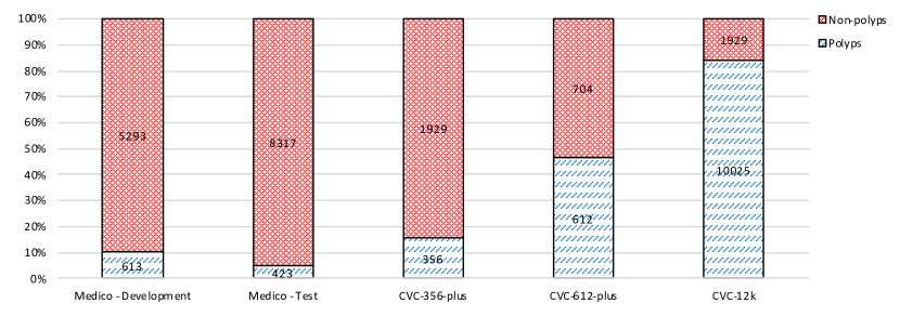
Figure 7. Ratios of findings to non-findings in the datasets (polyp/non-polyp). The X-axis represents the different datasets used for the binary classification. The Y-axis represents the percentage of polyps and non-polyps. The numbers inside the bars show the actual number of polyps and non-polyps images.

5.2. Analyzing results

We discuss our results in two main sections: 1) the 16 class classification task based on the 2018 Medico Task and 2) the polyps and non-polyps classification task to analyze generalizability of ML models.

5.2.1. 16-class classification

In this 16-class classification task, the training dataset of the 2018 Medico Task was split into a $70\%$ training dataset and a $30\%$ validation dataset. Then, the test data given by the organizers was used to test the performance of five methods for classifying 16 classes of the GI tract findings.

Table 4. Evaluation results of the 2018 Medico Task (as provided by the organizers of the 2018 Medico Task) (Thambawita et al., 2018) for the five methods used in this article. Based on the official results, method 5 was the best one based on the MCC score.

Method	REC	PREC	SPEC	ACC	MCC	F1
1	0.8457	0.8457	0.9897	0.9807	0.8353	0.8456
2	0.8457	0.8457	0.9897	0.9807	0.8350	0.8457
3	0.9376	0.9376	0.9958	0.9922	0.9335	0.9376
4	0.9400	0.9400	0.9960	0.9925	0.9360	0.9400
5	0.9458	0.9458	0.9964	0.9932	0.9421	0.9458

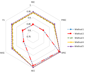
Figure 8. Performance comparison of all five classification models for the 16 classes of the 2018 Medico test dataset. Method 1 and 2 are similar in results but different from the other three methods (note that measurements start from $0.75$).

Table 5. Confusion matrix of method 5 (our best model) based on the Medico test dataset. The diagonal value represents true predictions (number of images) of the model. A to P are the classes corresponding to the class names in the first column. Most confusion can be observed between class B and C, and class D and E. Looking at the images shows that they are quite similar in their visual features (colors, texture, etc.)

		Actual class
		A	B	C	D	E	F	G	H	I	J	K	L	M	N	O	P
Predicted class	Ulcerative-colitis (A)	500	-	-	-	-	-	-	-	39	-	3	-	1	1	-	7
	Esophagitis (B)	3	432	48	-	-	-	-	-	-	-	-	-	-	-	-	-
	Normal-z-line (C)	1	121	513	-	-	-	-	-	-	-	-	-	1	-	-	-
	Dyed-lifted-polyps (D)	1	-	-	522	31	-	-	-	-	-	2	-	-	-	-	34
	Dyed-resection-margins (E)	-	-	-	33	532	-	-	-	-	-	1	-	-	-	-	17
	Out-of-patient (F)	-	-	-	-	1	5	-	-	-	-	-	-	-	-	-	-
	Normal-pylorus (G)	3	3	2	-	-	-	559	-	-	-	2	-	-	-	-	-
	Stool-inclusions (H)	-	-	-	-	-	-	-	501	7	-	-	-	-	-	-	-
	Stool-plenty (I)	1	-	-	-	-	-	-	-	1918	-	-	-	-	-	-	1
	Blurry-nothing (J)	1	-	-	-	-	-	-	-	1	37	-	-	-	-	-	-
	Polyps (K)	10	-	-	1	-	-	1	-	-	-	358	6	-	1	-	46
	Normal-cecum (L)	18	-	-	-	-	-	-	-	-	-	6	578	-	-	-	2
	Colon-clear (M)	1	-	-	-	-	-	-	5	-	-	-	-	1063	-	1	-
	Retroflex-rectum (N)	3	-	-	-	-	-	-	-	-	-	2	-	-	188	1	-
	Retroflex-stomach (O)	-	-	-	-	-	-	1	-	-	-	-	-	-	2	395	1
	Instruments (P)	-	-	-	-	-	-	-	-	-	-	-	-	-	-	-	165

We evaluated our five models based on the results collected by the organizers. This evaluated results of the main five models are tabulated in Table  4. With an MCC score of 0.9421, method 5 showed the best performance for classifying the 16 classes of GI tract findings. However, our GF-based approaches did not show results competitive with the DNN methods. The GF model introduced in method 1 could reach an MCC score of 0.8353. This result showed the best performance record for a GF-based method. A clear performance difference between GF-based methods and the DNN-based methods can be seen as depicted in Figure 8. In this plot, we compared this performance difference using six performance measures: Recall (REC), Precision (PREC), Specificity (SPEC), Accuracy (ACC), MCC and F-score (F1). According to this plot, it is clear that the areas of the hexagons covered by the GF methods are smaller than the areas covered by DNN methods. With these results, it implies that three DL methods outperform two GF methods.

The CM of method 5 collected from the organizers of the 2018 Medico Task is tabulated in Table 5 for the in-depth investigation. According to the CM, we can identify two main bottlenecks to improve the performance of method 5. The first one is misclassification between esophagitis and normal-z-line, and the second one is misclassification between dyed-lifted-polyps and dyed-resection-margins. Therefore, images from these classes were manually examined to identify the reasons for these misclassifications. For the conflict between esophagitis and normal-z-line, the reason is very close locations of these two landmarks in the GI tract. On the other hand, the confusion between dyed-lifted-polyps vs. dyed-restrictions caused because of the same color patterns and the same texture structures of both types of images. With these limitations, method 5 showed the best performance with an MCC of $0.9421$, which was the important measurement to win the 2018 Medico Task. Based on the MCC value, we won second place in the 2018 Medico Task. The winning team (Hoang et al., 2018) relabeled the development dataset and also generated more images out of the provided instruments class by placing the instrument as a foreground over the images of dyed-lifted-polyps, dyed-resection-margins, and ulcerative colitis to balance the instrument class for improving the performance. However, we developed the model by only using the images provided by the task organizers for a fair comparison of the approaches with the limited dataset. Then, our next experiments were conducted to find the re-usability of these well-performed models in different datasets with polyps and non-polyps categories (subcategories of the 16 classes of primary tasks).

5.2.2. Polyp and non-polyp classification using the pre-trained models

The following analysis was performed to identify the polyp classification ability of our five models on the same test dataset and different CVC datasets. The 16-class classification results collected from the Medico Task organizers were analyzed to calculate polyp detection performance in the Medico test data. Moreover, our models were tested with CVC-356-plus, CVC-612-plus, and CVC-12k datasets without any modifications to the five models to compare the performance of polyp detection.

According to the correct and incorrect classifications of polyps and non-polyps in the test datasets, the first large column of Table 6 was calculated to measure the polyps detection performance of five models. In this evaluation process, all the 15 classes except the polyp class were considered as the non-polyp classification because the number of outputs is 16 in the first models. For comparison, the MCC values of these tests are plotted in Figure 9. This graph shows that the polyp detection performance of the same dataset (the testing dataset of Medico Task) is higher than on the completely new datasets (CVC-356-plus, CVC-612-plus, and CVC-12k) for both the GF-based approaches and the DNN approaches. This is the first analysis, and we emphasize that it shows that researchers need to do cross-dataset evaluations to prove the real capabilities of ML models.

Table 6. Polyp classification results with and without retraining for all datasets and methods (column two M=Method). For training, 2018 Medico - development data was used. We can observe that for some datasets, retraining seems to improve the performance.

		Without retraining						With retraining to 2 class classification
	M	REC	PREC	SPEC	ACC	MCC	F1	REC	PREC	SPEC	ACC	MCC	F1
Test Dataset	1	0.7834	0.4899	0.9635	0.9558	0.5987	0.6028	0.9550	0.9630	0.6740	0.9553	0.5430	0.9590
	2	0.7834	0.4899	0.9635	0.9558	0.5987	0.6028	0.9540	0.9630	0.6840	0.9537	0.5400	0.9580
	3	0.9733	0.8088	0.9897	0.9890	0.8819	0.8835	0.9813	0.6577	0.9772	0.9773	0.7934	0.7876
	4	0.9599	0.8467	0.9922	0.9908	0.8969	0.8997	0.9813	0.7384	0.9845	0.9843	0.8440	0.8427
	5	0.9572	0.8463	0.9922	0.9907	0.8954	0.8984	0.9706	0.7516	0.9857	0.9850	0.8470	0.8471
CVC-356-plus	1	0.3089	0.1053	0.5158	0.4835	$-$0.127	0.1571	0.8450	0.7990	0.1700	0.8446	0.0750	0.7780
	2	0.3089	0.1053	0.5158	0.4835	$-0.127$	0.1571	0.8510	0.8420	0.2070	0.8512	0.1930	0.7930
	3	0.7865	0.3738	0.7569	0.7615	0.4198	0.5068	0.8118	0.5547	0.8797	0.8691	0.5978	0.6591
	4	0.6713	0.4003	0.8144	0.7921	0.4010	0.5016	0.6517	0.4150	0.8305	0.8026	0.4068	0.5071
	5	0.6685	0.4837	0.8683	0.8372	0.4737	0.5613	0.6713	0.6408	0.9305	0.8902	0.5906	0.6557
CVC-612-plus	1	0.7696	0.7969	0.8295	0.8016	0.6008	0.7830	0.6980	0.8070	0.6530	0.6983	0.4740	0.6590
	2	0.7696	0.7969	0.8295	0.8016	0.6008	0.7830	0.7220	0.8170	0.6800	0.7218	0.5140	0.6910
	3	0.8415	0.6242	0.5597	0.6907	0.4137	0.7168	0.8382	0.6136	0.5412	0.6793	0.3932	0.7086
	4	0.8627	0.6559	0.6065	0.7257	0.4803	0.7452	0.8578	0.6890	0.6634	0.7538	0.5265	0.7642
	5	0.8137	0.6501	0.6193	0.7097	0.4379	0.7228	0.8007	0.7061	0.7102	0.7523	0.5104	0.7504
CVC-12k	1	0.4858	0.8391	0.5158	0.4907	0.0012	0.6154	0.1650	0.7880	0.8370	0.1651	0.0130	0.0530
	2	0.4858	0.8391	0.5158	0.4907	0.0012	0.6154	0.1650	0.8210	0.8380	0.1699	0.0290	0.0630
	3	0.6112	0.9289	0.7569	0.6347	0.2722	0.7373	0.6033	0.9631	0.8797	0.6479	0.3558	0.7419
	4	0.6236	0.9458	0.8144	0.6544	0.3241	0.7517	0.6459	0.9519	0.8305	0.6757	0.3539	0.7696
	5	0.5936	0.9591	0.8683	0.6379	0.3401	0.7333	0.5576	0.9766	0.9305	0.6178	0.3595	0.7099

From the first column of Table 6 and Figure 9, it is clear that the performance of the GF methods for different datasets (CVC-356plus, CVC-612-plus, and CVC-$(356$+$612$) dataset) is unpredictable because it presents huge value fluctuations in the graph with negative MCC value. This shows the incapability of GF methods to make predictions on different datasets. The negative values of MCC in this experiment like $-0.127$ for the CVC-356-plus dataset indicate that there is no agreement or only a not relevant relationship between target and prediction. An MCC around 0 would mean that the classifier is deciding random and MCCs above 0 would indicate correct classification. The closer to -1 or 1 the stronger is the indication for begin wrong or correct, respectively. However, the polyp detection performance of the GF-based methods in the CVC-612-plus dataset outperforms the DNN methods with the MCC value of 0.6008 while the best DNN method shows the MCC value of 0.4803. This prediction accuracy of the GF methods can be identified as an erroneous prediction because the performance of this method for the other two CVC datasets shows poor MCC scores than the DNN based approaches. Moreover, the DNN based approaches show considerable steady MCC values for all new datasets, and it implies that DNN methods are more generalizable than the GF methods.

Because the performance gap between the 16-class classification and polyps classification showed differences, we retrained our models to classify only the polyps and non-polyps classes. Therefore, our next experiments were performed to test how retraining our five ML models to classify polyps and non-polyps will influence the performance.

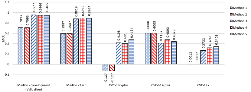
Figure 9. Polyps and non-polyps classification capabilities (based on MCC) of all five methods which were trained using 2018 Medico - development data to classify 16 classed. For most cases method 3 to 5 performs best. For CVC-612-plus test data, methods 1 and 2 are best performing.

For the retraining experiments, we first retrained the two GF methods with new ARFF files generated for polyps and non-polyps categories. Second, in the retraining stage of the three DNN methods, we changed only the last layer into two outputs. However, we did not change the loss function from categorical cross-entropy into binary cross-entropy because two-class categorical cross-entropy is equal to binary cross-entropy. Moreover, we retained the original optimization functions as it is. Then, we retrained all five models using the same Medico dataset, which has only polyps and non-polyps classes. At the end, the results of these experiments are tabulated in the right columns of Table 6.

The results in Table 6 show that it can be difficult to evaluate the models and interpret the results after retraining for two class classification. All MCC values of the five methods tested on the CVC-356-plus data show improvements. Similarly, for the CVC-612-plus test data, method 4 and 5 show performance improvements from MCC values of $0.4803$ and $0.4379$ to $0.5265$ and $0.5104$, respectively. In contrast, methods 1, 2 and 3 show a performance drop which is indicated by MCC values 0.6008, 0.6008 and 0.4137 reduced to 0.4740, 0.5140 and, 0.3932, respectively. Therefore, we extended our experiment by introducing additional retraining options with the CVC-356-plus and CVC-612-plus datasets. After that, the retraining process can be categorized as retraining the models to classify polyps and non-polyps using 1) only the same Medico training dataset (as tabulated in Table 6), 2) the Medico dataset with the CVC-356-plus dataset, 3) the Medico dataset with the CVC-612-plus dataset, and 4) the Medico dataset with the CVC-356-plus and CVC-612-plus datasets. Then, our testing datasets are limited to two datasets: the Medico test dataset and the CVC-12k dataset. Results related to these new retraining processes can be seen in Table 7. When the models are trained using the balanced CVC-612-plus dataset in combination with the 2018 Medico development data, the DNN models show better MCC values ($0.8189$, $0.8555$, and $0.8606$) for methods 3, 4, and 5, respectively. This is true for the Medico test data and the two smaller CVC datasets. Moreover, the MCC values for the CVC-12k test data also achieves the best MCC values of $0.1421$, $0.1418$, and $0.1802$ for method 3, 4, and 5. An important observation from the CVC-12k dataset is also that looking at all other metrics but MCC and specificity could mislead to the assumption that the results are good. For example, scores above $0.8$ for accuracy which is often used as the only indicator for performance in similar studies.

Table 7. Evaluation results on using CVC-356-plus and CVC-612-plus combined as training data with retraining to classify polyps and non-polyps. The 2018 Medico test dataset and the CVC-12k dataset are the test datasets. Using the balanced CVC-612-plus as training data, we achieve the best results. Combining the CVC-356-plus and the CVC-612-plus does not improve the performance. Overall the performance is better on the Medico test dataset.

			Medico test data						CVC-12k
		M	REC	PREC	SPEC	ACC	MCC	F1	REC	PREC	SPEC	ACC	MCC	F1
Retraining datasets with Medico data	CVC-356-plus	1	0.9550	0.9610	0.6230	0.9549	0.5160	0.9570	0.5840	0.7040	0.3090	0.5836	$-0.084$	0.6320
		2	0.9520	0.9620	0.6710	0.9521	0.5260	0.9560	0.5810	0.7100	0.3360	0.5807	$-0.065$	0.6310
		3	0.9626	0.6630	0.9781	0.9775	0.7887	0.7852	0.8423	0.8565	0.2665	0.7494	0.1052	0.8493
		4	0.9599	0.7526	0.9859	0.9848	0.8427	0.8437	0.9192	0.8481	0.1441	0.7941	0.0810	0.8822
		5	0.9706	0.7773	0.9876	0.9868	0.8623	0.8633	0.8694	0.8507	0.2068	0.7625	0.0802	0.8599
	CVC-612-plus	1	0.9510	0.9590	0.6270	0.9508	0.4970	0.9540	0.5840	0.7030	0.3040	0.5842	$-0.087$	0.6320
		2	0.9530	0.9610	0.6430	0.9530	0.5160	0.9560	0.6400	0.6970	0.2240	0.6395	$-0.117$	0.6660
		3	0.9652	0.7092	0.9823	0.9816	0.8189	0.8177	0.9325	0.8546	0.1752	0.8103	0.1421	0.8918
		4	0.9572	0.7766	0.9877	0.9864	0.8555	0.8575	0.9336	0.8544	0.1731	0.8109	0.1418	0.8922
		5	0.9626	0.7809	0.9879	0.9868	0.8606	0.8623	0.9486	0.8571	0.1778	0.8242	0.1802	0.9005
	CVC-{356+612}	1	0.9500	0.9600	0.6480	0.9503	0.5050	0.9540	0.6180	0.6930	0.2280	0.6179	$-0.129$	0.6520
		2	0.9500	0.9610	0.6710	0.9503	0.5170	0.9550	0.7200	0.7010	0.1820	0.7199	$-0.105$	0.7100
		3	0.9733	0.5909	0.9699	0.9700	0.7458	0.7354	0.9537	0.8479	0.1109	0.8177	0.1028	0.8977
		4	0.9545	0.7596	0.9865	0.9851	0.8443	0.8460	0.9543	0.8463	0.0995	0.8164	0.0874	0.8971
		5	0.9599	0.7771	0.9877	0.9865	0.8571	0.8589	0.9278	0.8462	0.1239	0.7981	0.0699	0.8851

(a)

(a)

(b)

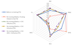
(b)

(c)

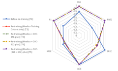
(c)

(d)

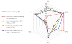
(d)

(e)

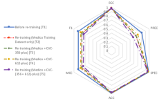
(e)

(f)

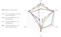
(f)

(g)

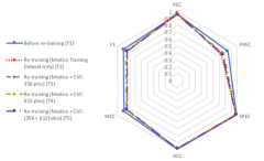
(g)

(h)

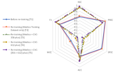
(h)

(i)

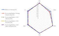
(i)

(j)

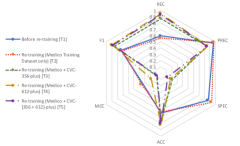
(j)

Figure 10. Polyps and non-polyps classification using the proposed ML methods: 1, 2, 3, 4 and 5. The first column (subfigures (a, c, e, g, i)) shows the results of the Medico test dataset and the second column(subfigures (b, d, f, h, j)) shows the results of the CVC-12k dataset. The methods are represented as following: a-b is for method 1, c-d is for method 2, e-f is for method 3, g-h is for method 4 and i-j is for method 5, respectively.

In the first comparison, we plotted performance changes for the retraining with the different training datasets and tested them on the Medico test dataset. The changes in the REC, PREC, SPEC, ACC, MCC and F1 values can be seen as hexagon plots in Figures 10a, 10c, 10e, 10g, and 10i which are corresponding to methods 1, 2 ,3, 4 and 5, respectively. In these plots, T1 is used to present performance values before retraining the ML models into two-class classification (binary classification). In this case, 15 classes except for the polyp class of the 16 classes were considered as the non-polyp class, and the polyp class is counted as the same polyp class. Furthermore, from T2 to T5 lines are used to present models with only two outputs. The T2 plot represents models’ performance for the retraining using the Medico training dataset. Similarly, T3, T4, and T5 represent the retraining process using the Medico dataset and the CVC-356-plus dataset, the Medico dataset and the CVC-612-plus dataset, and the Medico dataset, the CVC-356-plus dataset, and the CVC-612 dataset respectively.

In the second series of experiments in this session, the same experiments were performed and tested on the CVC-12k dataset. The results obtained from these experiments are tabulated in Tables 6 and 7. Then, relevant results from these tables are plotted in Figures 10b, 10d, 10f, 10h, and 10j. These plots use same line notations similar to the above experiments.

Using the plot series in Figure 10, we can examine the re-usability of ML models to classify polyps and non-polyps, which are sub-classes of the primary classes on the task. For example, if we compare plots in Figures 10a and 10b, then we can know that how method 1 performs to classify polyps and non-polyps within the test dataset same as the training dataset and within an entirely new dataset. While investigating these plots, the proportion of the number of polyps and non-polyps is an important factor in explaining the shape of these hexagon plots.

If we compare the GF methods (Figures 10a $-$ 10d ) and the DL methods (Figures 10e $-$ 10j), it is clear that DL methods outperforms the GF methods in both Medico Task and polyps classification task introduced in this paper. This implies that the DL methods are capable of extracting deep features that cannot be extracted by manual feature extraction methods used by the GF methods. With the retraining process in the GF methods, we can see performance differences between the Medico dataset and the CVC-12k dataset. The main conclusion that we make is that GF-based methods are not able to capture the underlying patterns that would allow for efficient classification; thus their performance is low.

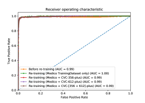
(a)

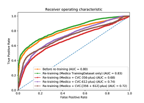
(b)

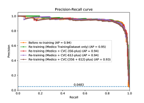
(c)

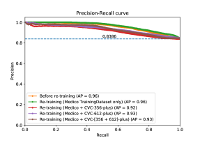
(d)

Figure 11. ROC and PRC curves for method 5 trained on the CVC-356-plus and CVC-612-plus dataset as mentioned in legends. Testing datasets are CVC-12k and the Medico test dataset. Overall good performance can be observed in both ROC and PRC. For CVC-12k the PRC curve shows the interesting case of a high random baseline for a biased dataset.

Plots in the first column and the second column in Figure 10 show completely different behaviors for the same retraining process when we use different test datasets. The test dataset for the first column comes from the same domain as the training data, and the test dataset for the second column comes from the completely new domain like CVC-12k dataset. To investigate these unusual performance changes, we generated and examined ROC curves and PRC curves for the best DNN model (method 5). The ROC and PRC curves for method 5 with the Medico test data (for the plot in Figure 10) are depicted in Figures 11a and 11c. Similarly, the ROC curve and the PRC curve for the method 5 with CVC-12k data (for the plot in Figure 10) are plotted in the Figures 11b and 11d.

Analysis of ROC curves is more robust for ML models that are used with balanced datasets, whereas PRC curves are more valuable for ML methods when the methods engage with imbalanced datasets. However, we have used both curves in this paper to investigate the behavior of these curves while we are using highly imbalanced datasets. Consequently, the PRC curves show completely different baseline values of $0.0483$ for the Medico test dataset and $0.8386$ for the CVC-12k dataset. The small baseline value arises in the plot in Figure 11c as a result of small polyps to the non-polyp proportion in the Medico test dataset. Conversely, the high baseline value in Figure 11d appears there as an effect on a high ratio of polyps to non-polyps.

To get a better understanding of the above plots, we selected the plots in Figures 10i and 10j, and ROC and PRC curves in Figure 11. With this selection, first, we analyze T1 and T2 from the hexagon plots and the corresponding ROC and PRC curves. While T2 shows a performance loss compared to T1 in Figure 10i, Figure 10j shows that T2 achieves a performance improvement over T1. Next, we look for the reasons for these performance changes.

In method 5, the model with the 16 outputs corresponding to T1 has 15 choices to classify non-polyp images. Similarly, the Medico test dataset has more non-polyp images compared to polyp images. On the other hand, the model corresponding to T2 has a $50\%$ chance to classify polyps as well as non-polyps. As a result, the model of T1 shows better performance than the model of T2 in Figure 10i. Because this shows a slight performance change, we cannot see the same difference in ROC and PRC curves in Figures 11a and 11c. In contrast, T2 in the plot in Figure 10j shows performance improvement when the model has a 50:50 chance for classifying polyps and non-polyps. This improvement occurred as a result of a large number of polyps in the CVC-12k dataset. The ROC and PRC curves in plots in Figures 11b and 11d shows this performance difference precisely. In other words, the model of T2 has a better chance of classifying polyps compared to the $1/16$ chance in the model of T1.

The retrained models corresponding to T3, T4 and T5 do not show considerable performance changes for the Medico test dataset as we can see from plots in Figures 10i, 11a, and 11c. Conversely, the retraining method used in T3, T4 and T5 for the CVC-12k dataset shows large performance changes in the plots in Figures 10j, 11b, and 11d. However, these methods show an overall performance loss. More comparisons about these plots are discussed in Section 6.

For the following experiments, we analyzed method 5 even further. The main focus of this analysis is to understand the behavior of the best model for training only the MLP versus training the whole DNN. In this experiment, we collected results for two main test datasets: the Medico test dataset and CVC-12k dataset. Then, we collected performance measures from the two training mechanisms:training only the MLP and training the whole DNN. Furthermore, results were tabulated in Table 8 and corresponding graphs were depicted in Figure 12 to analyze them.

Table 8. Method 5 - training only the MLP vs. complete-DNN. T - Additional training dataset which was added to the Medico dataset; T1 - Medico Dataset + CVC-356-plus, T2 - Medico Dataset + CVC-612-plus, T3 - Medico Dataset + CVC-356-plus + CVC-612-plus.

Test		Training only the MLP						Training the whole DNN
Data	T	REC	PREC	SPEC	ACC	MCC	F1	REC	PREC	SPEC	ACC	MCC	F1
Medico Test Data	T1	0.9572	0.5859	0.9698	0.9692	0.7357	0.7269	0.9706	0.7773	0.9876	0.9868	0.8623	0.8633
	T2	0.9599	0.7804	0.9879	0.9867	0.8591	0.8609	0.9626	0.7809	0.9879	0.9868	0.8606	0.8623
	T3	0.9626	0.6316	0.9749	0.9744	0.7684	0.7627	0.9599	0.7771	0.9877	0.9865	0.8571	0.8589
CVC-12k	T1	0.6984	0.8972	0.5842	0.6799	0.2184	0.7854	0.8694	0.8507	0.2068	0.7625	0.0802	0.8599
	T2	0.7588	0.8993	0.5583	0.7265	0.2565	0.8231	0.9486	0.8571	0.1778	0.8242	0.1802	0.9005
	T3	0.7614	0.8933	0.5272	0.7236	0.2352	0.8221	0.9278	0.8462	0.1239	0.7981	0.0699	0.8851

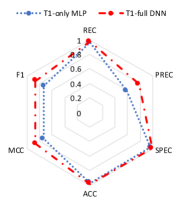
(a)

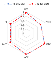
(b)

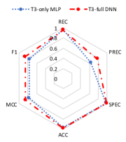
(c)

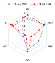
(d)

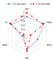
(e)

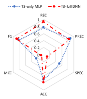
(f)

Figure 12. Behavior of the complex DNN method (method 5) while training only MLP compared to training the whole DNN. The first row shows the effects for these both cases when the test dataset is the Medico test data, and the second row shows the result when the test dataset is CVC-12k dataset. T1, T2, and T3 represent the training dataset used for the model. T1 - Medico training dataset + CVC356, T2 - Medico training dataset + CVC612, T3 - Medico training dataset + CVC356 + CVC612.

The first row of Figure 12 shows the differences in the performance of testing with the Medico test data. In the second row, it presents the performance changes for the CVC-12k dataset. The dotted lines in plots in Figure 12 represent the training only MLP. Similarly, the dash lines represent the training of the whole DNN. The three plots of each row represent results of retraining the model with the Medico training data and CVC-356-plus dataset, CVC-612-plus dataset and both CVC-356-plus, and CVC-612-plus datasets, respectively.

According to the plots in Figures 12a, 12b, and 12c, it is clear that retraining the whole DNN can be used to improve the overall performance of the DNN model because we can see performance improvement in these plots except in Figure 12b, which shows closely equal performance metrics. However, in test cases with the CVC-12k dataset, it shows a completely new behavior for retraining the whole DNN as depicted in Figures 12d, 12e, and 12f. These plots show large changes in the performance hexagons with considerable positive improvements for the recall and considerable performance loss for the specificity values. This experiment also shows that researchers could be misled by the performance monitoring process of DNN methods using a single dataset. In other words, according to the first row of the figure, researchers may conclude that retraining the whole DNN is a positive factor. However, the results of the second row prove that it is not always true by showing performance losses for the same technique.

The results presented in plots in Figures 12 show difficulties in adapting ML models for cross-dataset generalization with a different perspective. In that experiment, the performance loss in specificity, which is a parameter of reflecting TN detection, shows that method 5 is affected by imbalanced data in the CVC-12k dataset. The main reason for the effect is that the CVC-12k dataset contains a lower percentage of negative images compared to positive ones. This reflects an important factor to take into account when developing generalizable ML models which is that the ratio of negative and positive findings needs to be taken into account when looking at metrics. Metrics such as MCC are better suited to interpret results. In terms of ROC compared to PRC, the results show that PRC reflects the performance of the model more realistically than ROC.

6. Discussion

In this section, we discuss our findings and point out several important considerations for future research. Our discussion follows the same sequence as our contributions in this paper.

In our experiments, combinations of ResNet-152, Densenet-161, and an additional MLP produced the best result for the Medico 2018 dataset. The reported results from this model for Medico Task led us to hold second place based on the MCC values calculated by organizers, and there was only a tiny gap of around 0.0029. Furthermore, the winning team of this competition has used additional data items that were made by photo editing tools for the imbalanced classes such as the out-of-patients class. In contrast to this, our method 5 works well without using manually annotated data items because of the procedure we followed to implement and train that model. The procedure of implementing such a complex model is described step by step in Section 4.3 and anyone can follow these steps to get a well-performing DL model in a classification task.

In addition to the implementation and the procedure used in method 5, the data filling mechanism used to fill the out-of-patient imbalance class shows impressive performance gain. This method is preferred when one class has a small number of data items in a multi-class classification task. In our work, without annotating more data ourself which also requires the help of medical experts, we prefer to use random images from the Internet, as described in Section 5.1. This is an efficient way to add more data items without spending more time on manual annotation or creating synthetic data items. The above method works because the random images influence the ML models to make a wider range of possibilities to classify images into a particular class.

Dyed-lifted-polyps, dyed-resection-margins, esophagitis, and normal-z-line arose classification conflicts in our best method (method 5). If we could overcome these conflicts, then the model would perform better than the current recorded performance in the 2018 Medico Task. To identify the reasons for this classification conflicts, we manually investigated the images of these classes. If we compare sample images of dyed-lifted-polyps (Figure 1c), dyed-resection-margins (Figure 1d), esophagitis (Figure 1e), and normal-z-line (Figure 1i), then we can identify that this conflict caused as a result of similar texture and shapes of these images. To overcome this problem, researchers can select only the images that made conflict and train a new DL model to classify them into the correct classes. Then, this model can be added to the model introduced in method 5 using the property of its expandability.

Can we use our best DL model for real systems in hospitals to classify GI findings? Or can we use the state of the art ML classification models introduced by researchers in real applications? Towards answering this question, this paper focuses on deep evaluations of the proposed methods as one of the main contributions. Regularly, researchers present the performance of their classification models using only a test dataset, which was reserved from the dataset used to produce the training data. Also, they measure the performance selecting only a few measurements out of the REC, PREC, SPEC, ACC, MCC, and F1. However, we emphasize the requirements of an in-depth analysis of all of these six parameters at once to identify the real performance of ML models. Several of the works listed in Table 1 do not use this methodology as part of their evaluations. This makes it difficult to reason about the real-world performance of the proposed methods and how they compare with other methods. In this paper we also consider the importance of evaluating ML models with cross datasets.

Why do we need cross-dataset evaluations? To explain this requirement, we consider the research work done by Wang et al. (Wang et al., 2018). They presented an area under the receiver operating characteristic curve of 0.984 and a per-image sensitivity of $94.38$ for polyp detection. In our first look, these results show a good DL model. Similarly, our results in Figures 10i, 11a and 11c reflect the same impression in the first look because it shows excellent performance as a DL model. However, after analyzing cross-dataset performance for polyp detection with a completely new dataset like CVC-12k, we recognized that performance gain is not enough for applying it in real applications. Therefore, from this paper, we emphasize that researchers want to consider cross-dataset evaluations very thoroughly before applying their solutions in real-world applications. Otherwise, the selection bias, the capture bias, and the category bias (label bias) problems may appear in the results. Then, we may end up with the wrong conclusion about research works. All of these facts imply that more research works must be performed to improve the generalizability along with the performance improvement on a single dataset or single data source.

7. Conclusions

We have studied cross-dataset bias and evaluation metrics interpretation in machine learning (ML) using five methods and four different datasets within the field of Gastrointestinal (GI) endoscopy as respective use case. In particular, we performed an extensive study of ML models in the context medical applications based on a use-case of GI tract abnormality classification across different datasets. The main conclusion and resulting recommendation is that a multi-center or cross-dataset evaluation is important if not essential for ML models in the medical field to obtain a realistic understanding of the performance of such models in real world settings.

We found that the combination of the Deep Neural Network (DNN) ResNet-152 and Densenet-161 with an additional Multi-Layer Perceptron (MLP) performed best on both the validation and test datasets. This model shows that a combination of multiple pre-trained DNN models can have better capabilities to classify images into the correct classes because of their cumulative decision-making capabilities. We also proposed an evaluation method using six measures: Recall (REC), Precision (PREC), Specificity (SPEC), Accuracy (ACC), Matthews Correlation Coefficient (MCC), and F-score (F1). Moreover, we suggest that these measures should be presented all at once using hexagon plots that convey a complete view of real performance. We hope that these tools can enable a more realistic evaluation and comparison of ML methods.

Furthermore, we presented cross-dataset evaluations to identify the generalizability of our ML models emphasizing on the fact that achieving high scores for evaluation metrics does not always represent the real performance of ML models and should be interpreted with care. By evaluating the ML models with cross-datasets experiments, we showed the complexity of understanding the real functional performance of the models. The state of the art research works which perform classification cannot be used in practical applications because of their lack of generalizability. Based on the experimental results, we conclude that researchers should focus on implementing and researching generalizable ML models with cross-dataset evaluations. Rather than presenting metrics calculated from a simple training and testing split of the data, we suggest to always rely on cross-dataset evaluation to obtain a real-world representative indication of the model performance. This is especially important in a medical context since one has to make sure that the obtained models are reliable and not just perform well on a specific dataset.

Finally, we want point out that the lack of generalization, as evidenced by the poor result for cross-dataset evaluation presented in this article, rises the very important question: In the context of cross-dataset or multi-center studies, is it really possible to have generalizable ML models? This is something that we ourselves plan to investigate further in future work, and we hope that other researchers in computer science and medicine will do the same or at least have the question in their mind when performing similar studies.

- (1)
- Agrawal et al. (2017) Taruna Agrawal, Rahul Gupta, Saurabh Sahu, and Carol Y Espy-Wilson. 2017. SCL-UMD at the Medico Task-MediaEval 2017: Transfer Learning based Classification of Medical Images. In Proc. of MediaEval.
- Alexandre et al. (2008) Luís A Alexandre, Nuno Nobre, and João Casteleiro. 2008. Color and position versus texture features for endoscopic polyp detection. In Proc. of IEEE BMEI, Vol. 2. 38–42.
- Ameling et al. (2009) Stefan Ameling, Stephan Wirth, Dietrich Paulus, Gerard Lacey, and Fernando Vilarino. 2009. Texture-based polyp detection in colonoscopy. In Bildverarbeitung für die Medizin 2009. Springer, 346–350.
- Angermann et al. (2017) Quentin Angermann, Jorge Bernal, Cristina Sánchez-Montes, Maroua Hammami, Gloria Fernández-Esparrach, Xavier Dray, Olivier Romain, F. Javier Sánchez, and Aymeric Histace. 2017. Towards Real-Time Polyp Detection in Colonoscopy Videos: Adapting Still Frame-Based Methodologies for Video Sequences Analysis. In Proc. of CARE and CLIP. 29–41.
- Bernal et al. (2018) Jorge Bernal, Aymeric Histace, Marc Masana, Quentin Angermann, Cristina Sánchez-Montes, Cristina Rodriguez, Maroua Hammami, Ana Garcia-Rodriguez, Henry Córdova, Olivier Romain, Gloria Fernández-Esparrach, Xavier Dray, and Javier Sanchez. 2018. Polyp Detection Benchmark in Colonoscopy Videos using GTCreator: A Novel Fully Configurable Tool for Easy and Fast Annotation of Image Databases. In Proc. of CARS.
- Bernal et al. (2015) Jorge Bernal, F Javier Sánchez, Gloria Fernández-Esparrach, Debora Gil, Cristina Rodríguez, and Fernando Vilariño. 2015. WM-DOVA maps for accurate polyp highlighting in colonoscopy: Validation vs. saliency maps from physicians. Computerized Medical Imaging and Graphics 43 (2015), 99–111.
- Bernal et al. (2012) Jorge Bernal, Javier Sánchez, and Fernando Vilarino. 2012. Towards automatic polyp detection with a polyp appearance model. Pattern Recognition 45, 9 (2012), 3166–3182.
- Bernal et al. (2013) Jorge Bernal, Javier Sánchez, and Fernando Vilarino. 2013. Impact of image preprocessing methods on polyp localization in colonoscopy frames. In Proc. of IEEE EMBC. 7350–7354.
- Bernal et al. (2017) Jorge Bernal, Nima Tajkbaksh, Francisco Javier Sánchez, Bogdan J. Matuszewski, Hao Chen, Lequan Yu, Quentin Angermann, Olivier Romain, Bjørn Rustad, Ilangko Balasingham, Konstantin Pogorelov, Sungbin Choi, Debard Quentin, Lena Maier-Hein, Stefanie Speidel, Danail Stoyanov, Patrick Brandao, Henry Cárdova, Cristina Sánchez-Montes, Suryakanth Gurudu R., Gloria Fernández-Esparrach, Xavier Dray, Liang Jianming, and Aymeric Histace. 2017. Comparative validation of polyp detection methods in video colonoscopy: results from the MICCAI 2015 Endoscopic Vision Challenge. IEEE transactions on medical imaging 36, 6 (2017), 1231–1249.
- Borgli et al. (2018) Rune Johan Borgli, Pål Halvorsen, Michael Riegler, and Håkon Kvale Stensland. 2018. Automatic Hyperparameter Optimization in Keras for the MediaEval 2018 Medico Multimedia Task. In Proc. of MediaEval.
- Bottou (2010) Léon Bottou. 2010. Large-scale machine learning with stochastic gradient descent. In Proc. of COMPSTAT’2010. 177–186.
- Bray et al. (2018) Freddie Bray, Jacques Ferlay, Isabelle Soerjomataram, Rebecca L Siegel, Lindsey A Torre, and Ahmedin Jemal. 2018. Global cancer statistics 2018: GLOBOCAN estimates of incidence and mortality worldwide for 36 cancers in 185 countries. CA: a cancer journal for clinicians (2018).
- Cheng et al. (2011) Da-Chuan Cheng, Wen-Chien Ting, Yung-Fu Chen, and Xiaoyi Jiang. 2011. Automatic detection of colorectal polyps in static images. Biomedical Engineering: Applications, Basis and Communications 23, 05 (2011), 357–367.
- Contributors (2018) Torch Contributors. 2018. Torchvision Models. https://pytorch.org/docs/stable/torchvision/models.html [Online; Pytorch documentation].
- de Boer et al. (2005) Pieter-Tjerk de Boer, Dirk P. Kroese, Shie Mannor, and Reuven Y. Rubinstein. 2005. A Tutorial on the Cross-Entropy Method. International Journal of Annals of Operations Research (2005), 19–67.
- de Lange et al. (2018) Thomas de Lange, Pål Halvorsen, and Michael Riegler. 2018. Methodology to develop machine learning algorithms to improve performance in gastrointestinal endoscopy. World journal of gastroenterology 24, 45 (2018), 5057.
- Deng et al. (2009) Jia Deng, Wei Dong, Richard Socher, Li-Jia Li, Kai Li, and Li Fei-Fei. 2009. Imagenet: A large-scale hierarchical image database. In Proc. of IEEE CVPR. 248–255.
- Dias and Dias (2018) Danielle Dias and Ulisses Dias. 2018. Transfer learning with CNN architectures for classifying gastrointestinal diseases and anatomical landmarks. In Proc. of MediaEval.
- Doetsch et al. (2009) Patrick Doetsch, Christian Buck, Pavlo Golik, Niklas Hoppe, Michael Kramp, Johannes Laudenberg, Christian Oberdörfer, Pascal Steingrube, Jens Forster, and Arne Mauser. 2009. Logistic model trees with auc split criterion for the kdd cup 2009 small challenge. In Proc. of KDD-Cup. 77–88.
- Dollár et al. (2009) Piotr Dollár, Christian Wojek, Bernt Schiele, and Pietro Perona. 2009. Pedestrian detection: A benchmark. (2009).
- Friedman et al. (2000) Jerome Friedman, Trevor Hastie, and Robert Tibshirani. 2000. Additive logistic regression: a statistical view of boosting (with discussion and a rejoinder by the authors). The annals of statistics 28, 2 (2000), 337–407.
- Hall et al. (2009) Mark Hall, Eibe Frank, Geoffrey Holmes, Bernhard Pfahringer, Peter Reutemann, and Ian H Witten. 2009. The WEKA data mining software: an update. ACM SIGKDD explorations newsletter (SIGKDD Explor. Newsl.) 11, 1 (2009), 10–18.
- He et al. (2016) Kaiming He, Xiangyu Zhang, Shaoqing Ren, and Jian Sun. 2016. Deep residual learning for image recognition. In Proc. of IEEE CVPR. 770–778.
- Hicks et al. (2018) Steven A Hicks, Pia H Smedsrud, Pål Halvorsen, and Michael Riegler. 2018. Deep Learning Based Disease Detection Using Domain Specific Transfer Learning. In Proc. of MediaEval.
- Hoang et al. (2018) Trung-Hieu Hoang, Hai-Dang Nguyen, and Thanh-An Nguyen. 2018. An application of Residual Network and Faster - RCNN for Medico: Multimedia Task at MediaEval 2018. In Proc. of MediaEval.
- Huang et al. (2017) Gao Huang, Zhuang Liu, Laurens Van Der Maaten, and Kilian Q Weinberger. 2017. Densely Connected Convolutional Networks. In Proc. of IEEE CVPR. 2261–2269.
- Hwang et al. (2007) Sae Hwang, JungHwan Oh, Wallapak Tavanapong, Johnny Wong, and Piet C De Groen. 2007. Polyp detection in colonoscopy video using elliptical shape feature. In Proc. of the IEEE ICIP, Vol. 2. 465–468.
- Iakovidis et al. (2005) Dimitrios K Iakovidis, Dimitrios E Maroulis, Stavros A Karkanis, and A Brokos. 2005. A comparative study of texture features for the discrimination of gastric polyps in endoscopic video. In Proc. of IEEE CBMS. 575–580.
- Iwahori et al. (2013) Yuji Iwahori, Takayuki Shinohara, Akira Hattori, Robert J Woodham, Shinji Fukui, Manas Kamal Bhuyan, and Kunio Kasugai. 2013. Automatic Polyp Detection in Endoscope Images Using a Hessian Filter. In Proc. of MVA, Vol. 13. 21–24.
- Jha et al. (2020) Debesh Jha, Pia Smedsrud, Michael Riegler, Pål Halvorsen, Thomas de Lange, Dag Johansen, and Håvard Johansen. 2020. Kvasir-SEG: A Segmented Polyp Dataset. In Proc. of MMM. 1–12.
- Jia and Meng (2017) Xiao Jia and Max Q-H Meng. 2017. Gastrointestinal bleeding detection in wireless capsule endoscopy images using handcrafted and CNN features. In Proc. of IEEE EMBC. 3154–3157.
- Karkanis et al. (2003) Stavros A Karkanis, Dimitrios K Iakovidis, Dimitrios E Maroulis, Dimitris A. Karras, and M Tzivras. 2003. Computer-aided tumor detection in endoscopic video using color wavelet features. IEEE Transactions on Information Technology in Biomedicine 7, 3 (2003), 141–152.
- Khan and Tahir (2018) Zeshan Khan and Muhammad Atif Tahir. 2018. Majority voting of Heterogeneous Classifiers for finding abnormalities in the Gastro-Intestinal Tract. In Proc. of MediaEval.
- Khosla et al. (2012) Aditya Khosla, Tinghui Zhou, Tomasz Malisiewicz, Alexei Efros, and Antonio Torralba. 2012. Undoing the Damage of Dataset Bias. In Proc. of ECCV.
- Kingma and Ba (2014) Diederik P Kingma and Jimmy Ba. 2014. Adam: A method for stochastic optimization. arXiv preprint arXiv:1412.6980 (2014).
- Kirkerød et al. (2018) Mathias Kirkerød, Vajira Thambawita, Michael Riegler, and Pål Halvorsen. 2018. Using preprocessing as a tool in medical image detection. In Proc. of MediaEval.
- Ko and Tahir (2018) Tobey-Gu Zhonglei Ko, H. and Liu Yang Tahir. 2018. Weighted Discriminant Embedding: Discriminant Subspace Learning for Imbalanced Medical Data Classification. In Proc. of MediaEval.
- Landwehr et al. (2005) Niels Landwehr, Mark Hall, and Eibe Frank. 2005. Logistic model trees. Machine learning 59, 1-2 (2005), 161–205.
- Leufkens et al. (2012) AM Leufkens, MGH van Oijen, FP Vleggaar, and PD Siersema. 2012. Factors influencing the miss rate of polyps in a back-to-back colonoscopy study. Endoscopy 44, 05 (2012), 470–475.
- Li and Meng (2012) Baopu Li and Max Q-H Meng. 2012. Tumor recognition in wireless capsule endoscopy images using textural features and SVM-based feature selection. IEEE Transactions on Information Technology in Biomedicine 16, 3 (2012), 323–329.
- Lieberman (2005) David Lieberman. 2005. Quality and colonoscopy: a new imperative. Gastrointestinal endoscopy 61, 3 (2005), 392–394.
- Lux et al. (2016) Mathias Lux, Michael Riegler, Pål Halvorsen, Konstantin Pogorelov, and Nektarios Anagnostopoulos. 2016. LIRE: open source visual information retrieval. In Proc. of ACM MMSys. 30.
- Mamonov et al. (2014) Alexander V Mamonov, Isabel N Figueiredo, Pedro N Figueiredo, and Yen-Hsi Richard Tsai. 2014. Automated polyp detection in colon capsule endoscopy. IEEE transactions on medical imaging 33, 7 (2014), 1488–1502.
- Mori and Kudo (2018) Yuichi Mori and Shin-ei Kudo. 2018. Detecting colorectal polyps via machine learning. Nature biomedical engineering 2, 10 (2018), 713.
- Naqvi et al. (2017) Syed Sadiq Ali Naqvi, Shees Nadeem, Muhammad Zaid, and Muhammad Atif Tahir. 2017. Ensemble of Texture Features for Finding Abnormalities in the Gastro-Intestinal Tract. In Proc. of MediaEval.
- Ostroukhova et al. (2018) Olga Ostroukhova, Konstantin Pogorelov, Michael Riegler, Duc-Tien Dang-Nguyen, and Pål Halvorsen. 2018. Transfer learning with prioritized classification and training dataset equalization for medical objects detection. In Proc. of MediaEval.
- Park et al. (2012) Sun Young Park, Dustin Sargent, Inbar Spofford, Kirby G Vosburgh, and Y A-Rahim. 2012. A colon video analysis framework for polyp detection. IEEE Transactions on Biomedical Engineering 59, 5 (2012), 1408.
- Petscharnig et al. (2017) Stefan Petscharnig, Klaus Schöffmann, and Mathias Lux. 2017. An Inception-like CNN Architecture for GI Disease and Anatomical Landmark Classification. In Proc. of MediaEval.
- Pogorelov et al. (2018a) Konstantin Pogorelov, Olga Ostroukhova, Mattis Jeppsson, Håvard Espeland, Carsten Griwodz, Thomas de Lange, Dag Johansen, Michael Riegler, and Pål Halvorsen. 2018a. Deep Learning and Hand-crafted Feature Based Approaches for Polyp Detection in Medical Videos. In Proc. of IEEE CBMS. 381–386.
- Pogorelov et al. (2017a) Konstantin Pogorelov, Kristin Ranheim Randel, Thomas de Lange, Sigrun Losada Eskeland, Carsten Griwodz, Dag Johansen, Concetto Spampinato, Mario Taschwer, Mathias Lux, Peter Thelin Schmidt, Michael Riegler, and Pål Halvorsen. 2017a. Nerthus: A bowel preparation quality video dataset. In Proc. of ACM MMSys. 170–174.
- Pogorelov et al. (2017b) Konstantin Pogorelov, Kristin Ranheim Randel, Thomas de Lange, Sigrun Losada Eskeland, Carsten Griwodz, Dag Johansen, Concetto Spampinato, Mario Taschwer, Mathias Lux, Peter Thelin Schmidt, Michael Riegler, and Pål Halvorsen. 2017b. Nerthus: A Bowel Preparation Quality Video Dataset. In Proc. of ACM MMSYS. 170–174.
- Pogorelov et al. (2017c) Konstantin Pogorelov, Kristin Ranheim Randel, Carsten Griwodz, Sigrun Losada Eskeland, Thomas de Lange, Dag Johansen, Concetto Spampinato, Duc-Tien Dang-Nguyen, Mathias Lux, Peter Thelin Schmidt, Michael Riegler, and Pål Halvorsen. 2017c. Kvasir: A multi-class image dataset for computer aided gastrointestinal disease detection. In Proc. of ACM MMSys. 164–169.
- Pogorelov et al. (2017d) Konstantin Pogorelov, Michael Riegler, Sigrun Losada Eskeland, Thomas de Lange, Dag Johansen, Carsten Griwodz, Peter Thelin Schmidt, and Pål Halvorsen. 2017d. Efficient disease detection in gastrointestinal videos–global features versus neural networks. An International Journal of Multimedia Tools and Applications 76, 21 (2017), 22493–22525.
- Pogorelov et al. (2018b) Konstantin Pogorelov, Michael Riegler, Pål Halvorsen, Thomas De Lange, Kristin Ranheim Randel, Duc-Tien Dang-Nguyen, Mathias Lux, and Olga Ostroukhova. 2018b. Medico Multimedia Task at MediaEval 2018. In Proc. of MediaEval.
- Pogorelov et al. (2017e) Konstantin Pogorelov, Michael Riegler, Pål Halvorsen, Carsten Griwodz, Thomas de Lange, Kristin Randel, Sigrun Eskeland, Dang Nguyen, Duc Tien, and Olga Ostroukhova. 2017e. A comparison of deep learning with global features for gastrointestinal disease detection. In Proc. of MediaEval.
- Pogorelov et al. (2018c) Konstantin Pogorelov, Michael Riegler, Pål Halvorsen, Thomas De Lange, Kristin Ranheim Randel, Duc-Tien Dang-Nguyen, Mathias Lux, and Olga Ostroukhova. 2018c. Medico Multimedia Task at MediaEval 2018. In proc. of MediaEval.
- Riegler et al. (2014) Michael Riegler, Martha Larson, Mathias Lux, and Christoph Kofler. 2014. How’how’reflects what’s what: content-based exploitation of how users frame social images. In Proc. of ACM MM. 397–406.
- Riegler et al. (2016) Michael Riegler, Mathias Lux, Carsten Griwodz, Concetto Spampinato, Thomas de Lange, Sigrun L Eskeland, Konstantin Pogorelov, Wallapak Tavanapong, Peter T Schmidt, Cathal Gurrin, Dag Johansen, Håvard Johansen, and Pål Halvorsen. 2016. Multimedia and medicine: Teammates for better disease detection and survival. In Proc. of ACM MM. 968–977.
- Riegler et al. (2017a) Michael Riegler, Konstantin Pogorelov, Sigrun Losada Eskeland, Peter Thelin Schmidt, Zeno Albisser, Dag Johansen, Carsten Griwodz, Pål Halvorsen, and Thomas De Lange. 2017a. From annotation to computer-aided diagnosis: Detailed evaluation of a medical multimedia system. ACM Transactions on Multimedia Computing, Communications, and Applications (TOMM) 13, 3 (2017), 26.
- Riegler et al. (2017b) Michael Riegler, Konstantin Pogorelov, Pål Halvorsen, Kristin Randel, Sigrun Losada Eskeland, Duc-Tien Dang-Nguyen, Mathias Lux, Carsten Griwodz, Concetto Spampinato, and Thomas Lange. 2017b. Multimedia for medicine: the medico Task at mediaEval 2017. In Proc. of MediaEval.
- Ruder (2016) Sebastian Ruder. 2016. An overview of gradient descent optimization algorithms. arXiv preprint arXiv:1609.04747 (2016).
- Russakovsky et al. (2015) Olga Russakovsky, Jia Deng, Hao Su, Jonathan Krause, Sanjeev Satheesh, Sean Ma, Zhiheng Huang, Andrej Karpathy, Aditya Khosla, Michael Bernstein, Alexander Berg C, and Li Fei-Fei. 2015. ImageNet Large Scale Visual Recognition Challenge. International Journal of Computer Vision (IJCV) 115 (2015), 211–252.
- Salzberg (1994) Steven L Salzberg. 1994. C4. 5: Programs for machine learning by j. ross quinlan. morgan kaufmann publishers, inc., 1993. Machine Learning 16, 3 (1994), 235–240.
- Shin and Balasingham (2017) Younghak Shin and Ilangko Balasingham. 2017. Comparison of hand-craft feature based SVM and CNN based deep learning framework for automatic polyp classification. In Proc. of IEEE EMBC. 3277–3280.
- Steiner et al. (2018) Michael Steiner, Mathias Lux, and Pål Halvorsen. 2018. The 2018 Medico Multimedia Task Submission of Team NOAT using Neural Network Features and Search-based Classification. In Proc. of MediaEval.
- Sumner et al. (2005) Marc Sumner, Eibe Frank, and Mark Hall. 2005. Speeding up logistic model tree induction. In Proc. of PKDD. 675–683.
- Sutskever et al. (2013) Ilya Sutskever, James Martens, George Dahl, and Geoffrey Hinton. 2013. On the importance of initialization and momentum in deep learning. In Proc. of ICML. 1139–1147.
- Tajbakhsh et al. (2015) Nima Tajbakhsh, Suryakanth R Gurudu, and Jianming Liang. 2015. Automatic polyp detection in colonoscopy videos using an ensemble of convolutional neural networks. In Proc. of IEEE ISBI. 79–83.
- Tajbakhsh et al. (2016a) Nima Tajbakhsh, Suryakanth R Gurudu, and Jianming Liang. 2016a. Automated polyp detection in colonoscopy videos using shape and context information. IEEE transactions on medical imaging 35, 2 (2016), 630–644.
- Tajbakhsh et al. (2016b) Nima Tajbakhsh, Jae Y Shin, Suryakanth R Gurudu, R Todd Hurst, Christopher B Kendall, Michael B Gotway, and Jianming Liang. 2016b. Convolutional neural networks for medical image analysis: Full training or fine tuning? IEEE transactions on medical imaging 35, 5 (2016), 1299–1312.
- Taschwer et al. (2018) Mario Taschwer, Manfred Jürgen Primus, Klaus Schoeffmann, and Oge Marques. 2018. Early and Late Fusion of Classifiers for the MediaEval Medico Task. In Proc. of MediaEval.
- Thambawita et al. (2018) Vajira Thambawita, Debesh Jha, Michael Riegler, Pål Halvorsen, Hugo Lewi Hammer, Håvard D Johansen, and Dag Johansen. 2018. The Medico-Task 2018: Disease Detection in the Gastrointestinal Tract using Global Features and Deep Learning. In Proc. of MediaEval.
- Torralba and Efros (2011) A. Torralba and A. A. Efros. 2011. Unbiased look at dataset bias. In Proc. of IEEE CVPR. 1521–1528.
- Vázquez et al. (2017) David Vázquez, Jorge Bernal, F. Javier Sánchez, Gloria Fernández-Esparrach, Antonio M. López, Adriana Romero, Michal Drozdzal, and Aaron C. Courville. 2017. A Benchmark for Endoluminal Scene Segmentation of Colonoscopy Images. Journal of Healthcare Engineering 2017 (2017).
- Von Karsa et al. (2012) L Von Karsa, J Patnick, and N Segnan. 2012. European guidelines for quality assurance in colorectal cancer screening and diagnosis.First Edition-Executive summary. Endoscopy 44, Suppl 3 (2012), SE1–SE8.
- Wang et al. (2018) Pu Wang, Xiao Xiao, Jeremy R Glissen Brown, Tyler M Berzin, Mengtian Tu, Fei Xiong, Xiao Hu, Peixi Liu, Yan Song, Di Zhang, Xue Yang, Liangping Li, Jiong He, Xin Yi, Jingjia Liu, and Xiaogang Liu. 2018. Development and validation of a deep-learning algorithm for the detection of polyps during colonoscopy. Nature biomedical engineering 2, 10 (2018), 741.
- Wang et al. (2014) Yi Wang, Wallapak Tavanapong, Johnny Wong, JungHwan Oh, and Piet C De Groen. 2014. Part-based multiderivative edge cross-sectional profiles for polyp detection in colonoscopy. IEEE Journal of Biomedical and Health Informatics 18, 4 (2014), 1379–1389.
- Wang et al. (2015) Yi Wang, Wallapak Tavanapong, Johnny Wong, Jung Hwan Oh, and Piet C De Groen. 2015. Polyp-alert: Near real-time feedback during colonoscopy. International Journal of Computer methods and programs in biomedicine 120, 3 (2015), 164–179.
- Yu et al. (2017) Lequan Yu, Hao Chen, Qi Dou, Jing Qin, and Pheng Ann Heng. 2017. Integrating online and offline three-dimensional deep learning for automated polyp detection in colonoscopy videos. IEEE journal of biomedical and health informatics 21, 1 (2017), 65–75.
- Yuan et al. (2018) Yixuan Yuan, Dengwang Li, and Max Q-H Meng. 2018. Automatic polyp detection via a novel unified bottom-up and top-down saliency approach. IEEE journal of biomedical and health informatics 22, 4 (2018), 1250–1260.
- Zeiler (2012) Matthew D Zeiler. 2012. ADADELTA: an adaptive learning rate method. arXiv preprint arXiv:1212.5701 (2012).
- Zhang et al. (2019) Xu Zhang, Fei Chen, Tao Yu, Jiye An, Zhengxing Huang, Jiquan Liu, Weiling Hu, Liangjing Wang, Huilong Duan, and Jianmin Si. 2019. Real-time gastric polyp detection using convolutional neural networks. PloS one 14, 3 (2019), e0214133.
- Zhang et al. (2017) Xu Zhang, Weiling Hu, Fei Chen, Jiquan Liu, Yuanhang Yang, Liangjing Wang, Huilong Duan, and Jianmin Si. 2017. Gastric precancerous diseases classification using CNN with a concise model. PloS one 12, 9 (2017), e0185508.
- Zhou et al. (2014) Mingda Zhou, Guanqun Bao, Yishuang Geng, Bader Alkandari, and Xiaoxi Li. 2014. Polyp detection and radius measurement in small intestine using video capsule endoscopy. In Proc. of IEEE BMEI. 237–241.