Aspects of GR-MHD in High-Energy Astrophysics

Abstract

This work focuses on some key aspects of the General Relativistic (GR) - magneto-hydrodynamic (MHD) applications in High-Energy Astrophysics. We discuss the relevance of the GR-HD counterparts formulation exploring the geometrically thick disk models and constraints of the GR-MHD shaping the physics of accreting configurations. Models of clusters of tori orbiting a central super-massive black hole (SMBH) are described. These orbiting tori aggregates form sets of geometrically thick, pressure supported, perfect fluid tori, associated to complex instability processes including tori collision emergence and empowering a wide range of activities related expectantly to the embedding matter environment of Active Galaxy Nuclei. Some notes are included on aggregates combined with proto-jets, represented by open cusped solutions associated to the geometrically thick tori. This exploration of some key concepts of the GR-MHD formulation in its applications to High-Energy Astrophysics starts with the discussion of the initial data problem for a most general Einstein-Euler-Maxwell system addressing the problem with a relativistic geometric background. The system is then set in quasi linear hyperbolic form, and the reduction procedure is argumented. Then, considerations follow on the analysis of the stability problem for self-gravitating systems with determined symmetries considering the perturbations also of the geometry part on the quasi linear hyperbolic onset. Thus we focus on the ideal GR-MHD and self-gravitating plasma ball. We conclude with the models of geometrically thick GR-HD disks gravitating around a Kerr SMBH in their GR-HD formulation and including in the force balance equation of the disks the influence of a toroidal magnetic field, determining its impact in tori topology and stability.

1 Introduction

High-Energy Astrophysics is characterized by several processes involving different attractors as stars and super-massive black holes (SMBHs). These strong attractors, among the most energetic objects in the Universe, are supposed to be the engines of the high-energy outbursts of matter and fields, including $\gamma$-rays and X-rays emissions. The modelizations of the related observations and the description of the engines empowering these processes are dealt with a great computer simulation effort and differently challenging analytical means. These studies also involve very complex issues related to the life of the attractor as the SMBH formations and the progenitor collapse towards the formations of the BH horizons, the energy extraction from BHs and BHs evolutions, the exact mechanism empowering accretion and jet emission. Even the identification of the BH through its (ADM) mass and spin is a debated issue. Many methods are connected to the accretion disk physics, dealing with luminosity, accretion rates, location of inner edge and energy extraction. All these approaches are in large extents model dependent, as the same definitions of key aspects of BHs accretion, as the disks inner edge, are not at all clearly established. Recent and fairly independent methods includes the Gravitational Wave detection. Others, still rather mysterious phenomena, related to BHs accretion are the high-frequency quasi periodic oscillations (QPOs) observed in non-thermal X-ray emission from compact objects.

Active Galactic Nucleai (AGNs) provide a rich scenario to observe SMBHs interacting with their environments. These embeddings can host the formation of BH accretion disks with a structured inner morphology, following evolution of the central BH attractor interacting with the surrounding masses during several accretion regimes occurred in the lifetime of non-isolated Kerr BHs. The inner structure of the orbiting disk may leave traces of chaotical, discontinuous accretion episodes in the form of matter remnants orbiting the central attractor producing sequences of orbiting toroids with strongly different features as different rotation orientations with respect to the Kerr BH. Consequently corotating and counterrotating accretion stages can be mixed. This situation has been modelled in Ringed accretion disks (RAD) in Pugliese&Montani (2015); Pugliese&Stuchlik (2015, 2016, 2017a, 2018b, 2018a, 2018c, 2019); Pugliese&Montani (2018d). Ringed disks are clusters of toroidal (thick disk) configurations centered on a single BH, and prescribed by barotropic models. The model strongly binds the fluid and BH characteristics providing indications on the situations where to search for RADs observational evidences. The instability and the RAD structure strongly depend on the dimensionless spin of the central spinning attractor. These systems, were developed in special cases as eRAD, that is RADs composed by tori sharing the same equatorial plane which is also their symmetry plane and the equatorial plane of the central attractor. The eRAD admits a number of the instability points related to onset of GR-HD-pressure -supported accretion which is generally limited to n=2. From phenomenological view point these structures have been connected to different processes, for example the obscuring and screening tori, possibly evident as traces (screening) in X-ray spectrum emission. More generally however, a RAD observational evidence is expected by the spectral features of AGNs X-ray emission shape, due to X-ray obscuration by one of the tori, providing a RAD fingerprint as a radially stratified emission profile. This discussion of tori accreting disks is the focus of a part of our investigations.

This work has been intended as a conceptual review from the problematic and fundamental topics of the GR-MHD (general relativistic magnetohydrodynamic) systems and relevance of their GR-HD counterparts in dealing with some of the complex aspects of the Relativistic Astrophysics. We review topics of GR-MHD setup for a diversified set of scenarios, particularly on regards of the problem of existence and uniqueness of the solutions and their stability –Sec. (2.1). Therefore we look into the problems related to the perturbation of the gravitational field in the self-gravitating systems, the thermodynamic conditions implied by these in Sec. (2.3), and the propagation of the constraints (addressed in a brief discussion in Sec. (2.1)). The constraints are treated in the context of the accretion disks and particularly in the constrained models of thick disks where the symmetries imply an annulment of the evolution equations –Sec. (3.2)-(3.3). We inspect the issue of the multiple accreting systems in Sec. (3.4).  A goal of this review is therefore to examine the validity of the assumptions on matter fields into constitutive equations and state equations–Sec. (2.1)-Sec. (2.2), the implications on fluids thermodynamics, Sec. (2.3), especially in the context of fixed symmetries in self-gravitating objects, and toroid symmetry on a fixed background- - Sec. (4).

This brief review is conveniently divided into two parts. We start addressing the general Einstein–Maxwell–Euler (EME) system. In the first part the discussion focuses on some fundamental aspects of the MHD when considered in its full GR formulations and the GR-HD counterparts for the description of accretion toroids around very compact objects. Part I, consisting of Sec. (2), includes a discussion of the initial data problem for a general EME system. The reduction procedure is implemented and the system is set in quasi linear hyperbolic form. Considerations follow on the analysis of the stability problem for self-gravitating systems with determined symmetries considering the perturbations also of the geometry part on the quasi linear hyperbolic onset.

More in details: in Sec. (2.1) we discuss the initial value problem and stability analysis for the GR-MHD systems, addressing the formulation of an initial value problem, the stability analysis for systems with a privileged direction of symmetry and the gauge conditions and techniques on stability analysis. (The self-gravitating fluid configuration we selected can be finalized in a spherical self-gravitating radially pulsating ball or characterized in a more complex combination of modes). Problem set-up and the equations of the GR-MHD systems are in Sec. (2.2) while in Sec. (2.3) thermodynamic considerations follows. Finally this first part concludes in Sec. (2.4) with a summary of the situation for the infinitely conductive plasma.

The review continues with part II, Sec. (3) and Sec. (4), in which we consider orbiting systems on a fixed background with simplifying conditions on the system of equations and symmetries, especially the accretion thick disks for very compact objects, where the gravitational part of the disk force balance equation dictates the geometry and has a predominant role in determining some basic characteristics of the systems. The aggregate of tori is modeled as a single orbiting configuration, by introducing a leading function governing the distribution of toroids around the black hole attractor. (Eventually, disks agglomerate composed by tilted tori can be seen, depending on the tori thickness, and other conditions on tori and a ringed, RAD, structure as (multipole) gobules of orbiting matter, with different toroidal spin orientations, covering the embedded central black hole). These systems are shown to include tori with emerging instability phase related to accretion onto the central black hole and can provide even an evaluation of quantities related to tori energetics such as the mass-flux, the enthalpy-flux, and the flux thickness, depending on the model parameters for tori composed of polytropic fluids (Pugliese&Stuchlik, 2019).

In details: The GR-HD systems of thick tori orbiting Kerr SMBHs are introduced in Sec. (3) where we start introducing the Kerr geometry in Sec. (3.1). The HD-"stationary" configurations for thick tori are presented in Sec. (3.2). Constraints, morphology and angular momentum distribution in the disks are discussed in Sec. (3.3). Multi-accretion processes, multi–orbiting structures and ringed accretion disks are the focus of Sec. (3.4). This second part of the review ends in Sec. (4) dealing with magnetized tori, considering toroidal magnetic field in multi-accreting tori.

The study of the GR-HD counterpart in providing constraints for the development of more complex systems was motivated by the fact that, despite all the complexity of GR-MRI (magneto-rotational-instability) basing accretion processes in many GR-MHD disks - many features and properties are well described globally and morphologically by the HD models(Shafee et al., 2008; Fragile et al., 2007; De Villiers&Hawley, 2002; Porth et al., 2017; Abramowicz&Fragile, 2013). We have considered the Polish doughnut (PD) model of thick disk for a perfect fluid, circularly orbiting around a black hole of Schwarzschild and Kerr, in an hydrodynamic and magnetohydrodynamic context, using the effective potential approach examined in detail for the hydrodynamical model in Pugliese et al. (2013) We used the solutions of the barotropic torus with a toroidal magnetic field discussed in Komissarov (2006); Montero et al. (2007). We have considered the magnetic contribution to the total pressure of the fluid as a perturbation of the effective potential for the exact full general relativistic part. Relativistic hydrodynamics proved a successful framework of analysis an frame of contraints for more refined systems. As illustrated in a number of diversified scenarios, the relativistic HD plays a major role also in the presence of magnetic fields.

2 On the GR-MHD and the ideal GR-MHD

General Relativistic Magnetohydrodynamic (GR-MHD) is a complex set up for the description of a wide number of different aspects of High Energy Physics and High Energy Astrophysics where the GR component of the MHD onset is relevant in determining the stability and morphology of the configurations. These systems comprise self-gravitating objects, where the GR is a part of the equations to be treated as variables and within the scheme of the perturbation analysis, and extended matter orbiting on fixed backgrounds. In this first part of the review we consider the general set-up adapted to general self-gravitating systems. Although the analysis of gravitating systems such as accretion disks are often analyzed with emerging self-gravity effects, in Secs (3) and (4) we focus on the disk gravitating around a spinning SMBH. Starting from a self-gravitating onset, equations and perturbations can be easily found in the fixed-background geometry case.

We start by considering systems described by the coupled EME equations, which include general relativistic magnetohydrodynamic (MHD) systems. The perturbation analysis of such systems, requiring numerical approaches, is often very complicated, even if often implemented with suitable assumptions on the symmetries and the dynamics. Generally, MHD models find different problematics when considered with gravity. Firstly there is the more general and fundamental issue of the well-posedness of the equations with regards to the system initial data problem. Secondly and connected to this first point is the onset of the stability analysis for systems with given symmetries. We explore the first point in Sec. (2.1).

GR-MHD is involved in a very large number phenomena of accretion disks physics, from the magnetosphere configuration to the BH energy extraction. In a variety of astrophysical scenarios the stability problem of plasma configurations is a crucial issue involved in several aspects of High-Energy Astrophysics, ranging from stellar objects to accretion disks and their associated processes, and grounding in many models the instabilities describing the accretion processes or the jet emission. On the other hand, it is also clear that different models of accretion disk systems and attractors, imply extremely different typical instabilities, ranging from the MRI (magneto-rotational-instability) processes for example applied to accretion, to PPI (Papaloizou-Pringle Instability), an instabilities typically of geometrically thick disks and often interacting with MRI, to the runaway instability. We discuss these aspects further in Sec. (3) and Sec. (4). Due to the complexity of the equations, the analysis of the stability and the shape of accretion disks and flows is often addressed by numerical methods. A key challenge in dealing with the construction of the numerical solutions is to reduce the system to an appropriate formulation of the well-posedness problem of the initial values and the stability problem. The system formulation should ensure the local and global existence problems (Pugliese&Kroon, 2012; Shibata&Sekiguchi, 2005; Baumgarte& Shapiro, 2003; Palenzuela et al., 2010; Anile89, ; Lichnerowicz, 1967; Disconzi, 2014; Radice et al., 2014; Anton et al., 2006).

In this section, and Sec. (3) for the analysis of accreting disks, we consider a barotropic equation of state (EoS). As we shall discuss in Sec. (2.3), when the fluid entropy is a constant of both space and time, an equation of state to link the pressure $p$ to the matter density $\rho$ can be given in the form $p=p(\rho)$ — (Pugliese&Kroon, 2012). In this analysis we restrict our discussion to the case of isotropic fluids, considering a one species particles fluid (sometimes known as simple fluid). It is assumed that there is no particle annihilation or creation leading to the equation of conservation of particle number. In parts of this discussion we shall assume a polytropic equation of state and a constant velocity of sound. To simplify the analysis of the stability problem of linear perturbations, it will be necessary to specify the form of the conduction current using the Ohm’s law. This assumption ensures that linear relation between the conduction current and the electric field holds. Thus considering isotropic fluids we can set a constant electrical conductivity coefficient for the fluid (plasma).

2.1 GR-MHD systems: initial value problem and stability analysis

Formulation of an initial value problem.

The formulation of a good initial value problem is a relevant issue of the MHD applications, including systems described in their GR reformulation for self-gravitating and orbiting systems. The formulation of an initial value problem is a necessary starting point for the construction of numerical solutions of the EME system. General Relativity admits itself an initial value problem formulation which is its own Cauchy problem. In the GR frame, prescribing initial data on a 3-dimensional hypersurface, one could reconstruct the spacetime associated to this initial data. Having a well initial value problem formulation implies some unquestionable advantages, it ensures the (local and global) existence and uniqueness of the solution, starting from initial data and secondly it allows a correct and convenient procedure for the stability analysis of certain reference solutions. Here we follow the procedure in Pugliese&Kroon (2012) implemented for GR-MHD system where this problem was addressed with the construction of a first order symmetric quasi-linear hyperbolic evolution system for the EME system (evolution equations) describing a charged ideal perfect fluid coupled to the Einstein field equations. The analysis in Pugliese&Kroon (2012) shows how the EME system admits a reduction procedure leading to symmetric hyperbolic evolution (first-order) equations and thus this automatically shows the local existence and uniqueness of the solutions for the system under consideration. The analysis we review in this section, is based on a $(1+3)$-tetrad decomposition, in order to ensure the symmetric hyperbolicity of the evolution equations implied by the Bianchi identity, and using tensor of rank 3 corresponding to the covariant derivative of the Faraday tensor as auxiliary function, making use of the Weyl tensor components as one of the unknowns. The system can be further reduced, assuming the case of a perfect fluid with infinite conductivity (ideal MHD) as a particular subcase, which applies to the study of plasmas in situations where a fluid is subjected to significant magnetic fields. This approach serves especially when the gravity is perturbed. The evolution equations have unique local solution (a solution that exists at least for a small interval of time), the solutions obtained from the Cauchy problem depend continuously on the values of initial data–conditions which are consistent with a well-posed initial value problem. The particular procedure adopted in this approach borrows from the discussion of the evolution equations for the Einstein-Euler system in Friedrich (1998); Friedrich&Rendall (2000); Friedrich (1996); Reula (1998), where a Lagrangian gauge was used (flow lines of the fluid fix the preferred time). However, there are in general different ways of dealing with the issue of Cauchy problem and stability especially when it concerns self-gravitating systems implying perturbation of the background. It is clear that in this special GR-MHD system the central equation is the Bianchi identity, intrinsically providing Weyl tensor evolution equations. This is borrowed from the analysis of the conformal Einstein-Maxwell system of (Friedrichs, 1991)–(see also for similar Ellis&van Elst (1998) frame formalism equations, while there are several formulations of the evolution equations of the EME system for the numerical computations especially for the conditions of ideal magnetohydrodynamics–(Baumgarte& Shapiro, 2003; Shibata&Sekiguchi, 2005; Etienne et al., 2010; Font, 2003)). In Baumgarte& Shapiro (2003) it makes use of an ADM formulation for the Einstein part of the system, which is known to have problems concerning hyperbolicity–(Friedrich, 1996). This hyperbolicity of the Einstein part of the system in an ADM formulation has been addressed in Shibata&Sekiguchi (2005); Etienne et al. (2010) using a BSSN formulation (BSSN equations are first order in time and second order in the spatial coordinates), and satisfied under certain additional conditions in vacuum the strong hyperbolicity– (Gundlach& Martín-García, 2006; Baumgarte& Shapiro, 2003; Alcubierre, 2008). Within further assumptions the local existence and uniqueness of solutions for these systems can be ensured–(Rendall, 2008). Nevertheless this is a mixed order system, also hard to implement in non-vacuum regions, for example in the EME systems.

The procedure should ensure the consistency of possible numerical approaches to the problems. On the other hand, the problem of the propagation of the constraints can be assumed satisfied at all time and then prove this result by fairly general arguments as discussed in Reula (1998, 1999). Moreover, the covariant and gauge–invariant perturbation formalism can be more conveniently adapted to spacetimes with some preferred spatial direction and possibly applied to the case of gravitational wave propagation by introducing a radial unit vector and decomposing all covariant quantities with respect to this (Clarkson, 2007; Marklund&Clarkson, 2005; Baumgarte& Shapiro, 2003). (In any case, for the linear perturbation analysis it is often useful, as done in Pugliese&Kroon (2012, 2016), to introduce a re-parameterized set of evolution equations based of a suitable combination of the radially projected shear and expansion. The resulting evolution system was then used in Pugliese&Kroon (2016) to analyse the stability problem for small linear perturbations of the background, thus the re-parameterized set of evolution equations can be collected in a proper symmetric hyperbolic form on which the perturbation to the first order of the variables can be discussed.). The set of evolution equations has to be complemented by the constraint and constitutive equations. One can consider isotropic fluids (where entropy is a constant of both space and time) and one species particle fluid (simple fluid) and at later steps of the analysis one can introduce a polytropic equation of state with a constant velocity of sound. To close the system of evolution equations it is necessary to specify the form of the conduction current. Accordingly, in Pugliese&Kroon (2012, 2016) the Ohm’s law was assumed so to obtain a linear relation between the conduction current and the electric field, with a constant electrical conductivity coefficient. Ultimately the pressure of the fluid $p$ and the charge density $\varrho_{C}$ can be assumed to be general functions of the matter density $\rho$, and the charge current $j_{c}$ a function of the electric field $E$.

Thus, summarizing , the GR-MHD system can then be casted in quasi linear symmetric hyperbolic evolution system by prescribing suitable initial data on an initial hypersurface. We focus on the properties of the evolution system.and the analysis of its linear stability, while for further aspects of the propagation of the constraints we refer to Pugliese&Kroon (2012) and in particular Reula (1998, 1999). Consequently, following Pugliese&Kroon (2012) we can write the evolution equations for the independent components of $n$ variables collected in the $n$-dimensional vector v, introduced to obtain a suitable symmetric hyperbolic evolution system of the form

$$\mathbf{A}^{0}\partial_{0}\textbf{{v}}-\mathbf{A}^{j}\partial_{j}\textbf{{v}}=\mathbf{B}\mathbf{v}.$$ (1)

Quantities in Eq. (1) $\mathbf{A}^{\mu}=\mathbf{A}^{0}(x^{\mu},{\mathbf{v}})$ are matrix-valued functions of the coordinates and the unknowns ${\mathbf{v}}$: $\mathbf{A}^{0}$ and $\mathbf{A}^{j}$ and B are smooth matrix valued functions of the coordinates $(t,x)$ and the variables v with the index $j$ associated to some spatial coordinates $x$. The system is symmetric hyperbolic if the matrices $\mathbf{A}^{0}$ and $\mathbf{A}^{j}$ are symmetric and if $\mathbf{A}^{0}$ is a positive-definite matrix. These evolution equations must be then complemented by constraint and the constitutive equations.

Stability analysis for systems with a privileged direction of symmetry

In presence of special symmetries as the spherical symmetry the problem can be addressed by means of an adapted $(1+1+2)$ decomposition. In the first step of a $(1+3)$ decomposition the various tensorial quantities and equations are projected along the direction of the observer comoving with the fluid and onto its orthogonal subspace. Quite often it is convenient to assume, to fix certain components of the connection especially in the self-gravitating systems, the timelike vector of the defined orthonormal frame to follow the matter flow lines (Lagrangian gauge) and also the vector fields tetrad to be Fermi transported in the direction of $U$–(Friedrich, 1998; Friedrich&Rendall, 2000). In Pugliese&Kroon (2012) a key feature of the analysis was the introduction of a further tensor $\psi_{abc}=\nabla_{a}F_{bc}$, where $F_{ab}$ is the Faraday tensor and $\nabla_{a}$ is the covariant derivative. This implies to write the evolution and constraining equations for the 3-rank tensor $\psi$ ensuring however the symmetric hyperbolicity of the propagation equations for the components of the Weyl tensor (which is actually decomposed into its electric and magnetic parts).

As we mentioned above this formalism and particularly the procedure adopted in Pugliese&Kroon (2012), providing the introduction of an auxiliary variable is particularly well suited to the study of the stability of more varied GR-MHD systems and including configurations characterized by some particular symmetries. Considered as an additional exemplification, we can take advantage of the presence of a privileged direction of symmetry in addressing the initial data problem and the stability analysis as well: the initial value formulation of GR-MHD discussed above can be used to discuss the stability of configurations characterized by certain symmetries, for example in spherically symmetric configurations. This approach however breaks the covariance of the equations by introducing coordinates and choosing a preferred timelike direction in the spacetime (thus prescribing a gauge choice). In fluid models the convenient natural timelike direction is given by the fluid flow-lines. The motivation behind the gauge choice is to obtain a closed (as many equations as unknowns) subsystem of evolution equations in symmetric hyperbolic form (this procedure is known as the hyperbolic reduction)–(Friedrich&Rendall, 2000). In this context, in Pugliese&Kroon (2016) by means of a $(1+1+2)$-tetrad formalism the linear stability of an Einstein-Maxwell perfect fluid configuration with a privileged direction of symmetry was examined. The nonlinear stability for the case of an infinitely conducting plasma was also considered. This system can model a self-gravitating ball of Maxwell matter fluid (stability problem for locally rotationally symmetric (LRS) solutions). More specifically, the analysis was restricted to isotropic fluid configurations and it was assumed a constant electrical conductivity coefficient $\sigma_{J}$ for the fluid (plasma). Consequently to these assumptions, the equations describing the evolution of the system were casted in quasi linear symmetric hyperbolic form.

A further interesting aspect of the application to this special system, is that the threshold for the emergence of the instability appears in both contracting and expanding systems (according to the kinematic expansion scalar $\Theta$). The system instabilities enlighten two ranges for the density of matter, and shear scalar $\Sigma$ along the privileged direction of the system. In conjunction with this setup, including the magnetic field but not dissipative effects, the stability analysis proved the instability emergence with unstable modes threshold, regulated by the conductivity parameter $\sigma_{J}$ and the speed of sound $v_{s}$. The stability conditions were strongly determined by the constitutive equations, the square of the velocity of sound and the electric conductivity, hence a complete classification and characterization of various stable and unstable configurations followed. (We note that the special case of an infinitely conducting plasma describes an adiabatic flow so that the entropy per particle is conserved along the flow lines–for a more specific discussion on the stability of spherically symmetric plasma see for example Horst (1990); Laskyand&Lun (2007); Viana et al. (1997); Guo&Tahvildar-Zadeh (1999).). The velocity of sound and the conductivity act in a different way for the systems according to different assumptions. Contracting systems with a fast contraction rate or expansion according to this threshold are certainly unstable. In the other cases instead the threshold is provided by the density values $\rho$, and the couple $(\Sigma,\Theta)$ in different ranges depending on $(\rho,v_{s},\sigma_{J})$. Then, a further aspect to underline in this context is that, as proved in Pugliese&Kroon (2016), the magnetic field does not have a specific role in determining the stability of the system, and the Maxwell field and the geometrical effects enclosed by the magnetic and electric part of the Weyl tensor. However, often in the handling of system equations, further simplifications are due. This is because even in simplest case the perturbed equations for the radially projected acceleration $\mathcal{A}$ is a rather complicated expression of the other variables and derivatives. Thus the necessity of a simplified form, grounded on some assumptions on the configuration (for example assuming a null radial acceleration for the reference solution, one can then fix the expansion of the 3-sheets and 2-sheets, the radial part of the shear of the 3-sheet, the twisting of the 2-sheet and the radial part of the vorticity of the 3-sheet, etc), leading to consider systems from different stability classes, where stability conditions bind mainly the expansion or contraction along the preferred direction with respect to different regimes of the radial shears.

First a symmetric hyperbolic system was written. The simplest example of a configuration with LRS symmetry is the spherical symmetric configurations. The assumption on the local symmetry of the system leads to a covariant decomposition of Einstein-Maxwell perfect fluid field equations extending the usual $(1+3)$-formalism to a convenient adapted $((1+1+2))--$formalism. In the $((1+1+2))$-formalism, it is assumed a further (spatial) vector field $n^{a}$. This assumption reduced the equations on the plane parallel and orthogonal to $n^{a}$, fixing the spatial vector on the privileged symmetry direction (in Pugliese&Kroon (2016) being the radial direction) at each point of LRS classes II space-times as described in Clarkson (2007) see also Laskyand&Lun (2007); Clarkson (2007); Betschart&Clarkson (2004); Burston (2008b); Burston&Lun (2008); Burston (2008a) and for a deeper and more general discussion about the MHD configurations in spherical symmetry, see Horst (1990); Laskyand&Lun (2007); Viana et al. (1997); Guo&Tahvildar-Zadeh (1999). It is clear that for spherically symmetric spacetimes (LSS), $n^{a}$ can naturally be taken to point in the radial direction of the spherical symmetry, which is therefore the system privileged direction of the system admitting a one–dimensional isotropy group. We precise that the covariantly split in $(1+1+2)$ procedure leads to scalars, vectors, and transverse-traceless 2-tensors, with respect to $n^{a}$– (Clarkson, 2007; Betschart&Clarkson, 2004). As we have mentioned earlier this formalism can be equally used for the analysis of the stability problem for the self-gravitating systems in Laskyand&Lun (2007) and the same formalism has been used to analyse self gravitating spherically symmetric charged perfect fluid configurations in hydrostatic equilibrium. One can consider the perturbations of the background or otherwise to fix the spacetime reducing the self–gravitating to an orbiting configuration on a fixed background, as we do in Sec. (3) and Sec. (4) for toroidal configurations. In Pugliese&Kroon (2016) the more general case was addressed considering perturbations of the gravitational part, in terms of scalars of the Weyl tensor, considering the symmetries preserved by the perturbation and assuming a constant velocity of sound and conductivity parameter. Considering the full gravito-electromagnetic effects, one can classify the solutions in terms of the scalars of the Weyl’s conformal tensor. The gravitational background must, in any case, have the same symmetries of LRS systems. In the approaches considered in Pugliese&Kroon (2016, 2012) the electromagnetic fields are considered through real vector functions.

On gauge conditions and techniques on stability analysis

The hyperbolic reduction developed for the general system in Lubbe&Kroon (2013); Pugliese&Kroon (2012) is independent of geometric gauge considerations. In a LRS spacetime any background quantities are scalars, implying that the vector and tensor quantities are automatically gauge invariant, under linear perturbations as a consequence of the Stewart-Walker lemma (Stewart&Walker, 1974; Clarkson, 2007). A number of simplified subsystems can be analyzed. (For example, in Pugliese&Kroon (2016) background configurations with a vanishing radial acceleration for the reference solution are considered, then exploring models with fixed values of particularly kinematic scalar, as the $(1+1+2)$-projected expansion, shear, twisting and the vorticity of the system). As done in Pugliese&Kroon (2012), to provide a suitable propagation equation used in Pugliese&Kroon (2016), an auxiliary field is used to rephrase the stability problem for small nonlinear perturbations of a background solution, for the fluid radial acceleration. This field corresponds to the derivative of the matter density projected along the radial direction. Then, a first order perturbation to $\mathbf{v}$ of the form $\mathbf{v}\mapsto\epsilon\mathring{\mathbf{v}}+\breve{\mathbf{v}}$ is assumed, where the parameter $\epsilon$ sets here the order of the perturbation and $\breve{\mathbf{v}}$ describes the (linear) perturbation of the background solution. Assuming the background variables $\mathring{\mathbf{v}}$ to satisfy the unperturbed system, an evolution system for the perturbations of the form $\mathring{\mathbf{A}}^{t}\partial_{t}\breve{\textbf{{v}}}-\mathring{\mathbf{A}}^{j}\partial_{j}\breve{\textbf{{v}}}=\mathring{\mathbf{B}}\breve{\mathbf{v}}$ was obtained. The core of the stability analysis, adapted from discussion in Reula (1999); Alho et al. (2017), consisted of the study of the background term $\mathring{\mathbf{B}}$ using some relaxed stability eigenvalue conditions. (This procedure could be used as first step towards the analysis of non-linear stability, under suitable circumstances). Then indirect methods based for example on the inspection of the characteristic polynomial can be used for the analysis of the eigenvalues. (In other words we study of the non principal part of the matrix $\mathring{\mathbf{B}}$ of the system using some relaxed stability eigenvalue conditions, establishing conditions where the linear instability occurs.). The reason for adopting indirect methods to explore the system stability is that the elements of matrix $\mathring{\mathbf{B}}$ are, in general, functions of the space and time coordinates and then adding a further complication to the analysis.

2.2 Problem set-up: the equations

Below we introduce the basic equations describing a relativistic charged perfect fluid coupled gravity, constituted by the EME system.

For reference we report below a summary of main notations and convection introduced along this discussion.

Remarks on notation and convection

The implementation of the $1+3$-formalism used in the present article follows the notation and conventions of Pugliese&Kroon (2012, 2016). The 4-dimensional metrics $g_{ab}$ has signature $(-,+,+,+)$. When more convenient, we also introduce a multiplicative constant $\epsilon=\pm$ in leaving the (pseudo-Riemannian) signature indeterminate in the first part of this review, precisely in Sec. (2) where we will deal with certain general aspects of the GR-MHD equations set without fixing the metric, therefore preferring an independent signature treatment. In the second part, Sec. (3) and Sec. (4) we will fix a precise geometric background, writing the line element for the geometry and fixing the signatures. The Latin indices $a,b,c...$ will denote spacetime tensorial indices taking the values $(0,1,2,3)$ while $i,j,k...$ will correspond to spatial frame indices ranging over $(1,2,3)$. The Levi-Civita covariant derivative of $g_{ab}$ will be denoted by $\nabla_{a}$. Whenever convenient, we use the semicolon notation. As usual, one has that $\nabla_{a}g_{bc}=g_{bc;a}=0$.

In what follows, the timelike vector field (flow vector) $U^{a}$ will describe the normalised future directed 4-velocity of the fluid. Fixing the signature such that $U^{a}U_{a}=-1$ (indices are raised and lowered with $g_{ab}$), the tensor $h^{ab}$ is the projector onto the three dimensional subspace orthogonal to $U^{a}$, thus, one has that $h^{a}{}_{b}=\delta^{a}{}_{b}+U^{a}U_{b},\quad h^{b}{}_{a}h^{a}{}_{c}=h^{b}{}_{c},\quad h^{a}{}_{b}h^{b}_{a}=3,\quad h^{a}{}_{b}U_{a}=0.$ Following the standard approach of $(1+3)$-formalisms, we split the first covariant derivative of $U^{b}$ as

$$\nabla_{a}U_{b}=\sigma_{ab}+\omega_{ab}+{\frac{1}{3}}\,\Theta h_{ab}-\dot{U}_{b}U_{a},$$ (2)

where $\sigma_{ab}\equiv D_{\langle b}U_{a\rangle}$ with $\sigma_{ab}U^{b}=0$, $\omega_{ab}\equiv D_{[a}U_{b]}$ with $\omega_{ab}U^{b}=0$, $\Theta\equiv D^{a}U_{a}$ and $\dot{U}_{a}=U^{b}\nabla_{b}U_{a}$ are, respectively, the shear and the vorticity tensors, the volume expansion scalar, and the 4–acceleration vector. We introduce the vorticity vector $\omega^{a}\equiv\epsilon^{abc}\omega_{bc}/2$ where $\epsilon_{abc}=U^{d}\epsilon_{dabc}$, $\epsilon_{abe}\epsilon^{abe}=6$ and $\epsilon_{dabc}$ stands for the totally antisymmetric tensor with $\epsilon_{0123}=\sqrt{-\det{g_{ab}}}$. Then, $\sigma_{ab}U^{a}=0=\omega_{ab}U^{a}=\dot{U}_{a}U^{a}$ by construction. In the above expressions, the operator $D_{a}$ corresponds to the 3-dimensional covariant derivative obtained from projecting the spacetime covariant derivative in the distribution orthogonal to $U_{b}$, for a generic 2-rank tensor $T_{bc}$, one has that $D_{a}T_{bc}=h^{s}{}_{a}h^{t}{}_{b}h^{p}{}_{c}T_{st;p}$, and $T_{st;p}=\nabla_{p}T_{st}$. For clarity, whenever necessary, projected indices of a tensor will be highlighted by $\langle\rangle$- brackets. For example, we write $T_{\langle ab\rangle}=h_{a}{}^{c}h_{b}{}^{d}T_{cd}$. Where $\dot{w}_{\langle a\rangle}\equiv h_{a}{}^{b}\dot{w}_{b}$ denotes the directional covariant derivative along the flow vector (Fermi derivative) and $D_{a}w_{b}\equiv h_{a}{}^{u}h_{b}{}^{v}\nabla_{u}w_{v}$ is the orthogonally projected covariant derivative of a vector.

Einstein-Euler-Maxwell equations:

We start by considering the following Einstein equations

$$G_{ab}=T_{ab}=T^{(f)}_{ab}+T^{(em)}_{ab}$$ (3)

the energy-momentum tensor $T_{ab}$ singles out the electromagnetic part $T^{(em)}_{ab}$ we discuss below and the fluid momentum tensor $T^{(f)}_{ab}=(\rho+p)U_{a}U_{b}-\epsilon\ pg_{ab}$ for the ideal fluid, while $\rho$ and $p$ are, respectively, the total energy density and pressure as measured by an observer moving with the fluid. The time-like vector field (flow vector) $U^{a}$ denotes the normalized future directed 4-velocity of the fluid. It satisfies $U^{a}U_{a}=\epsilon$. Associated to $U^{a}$ we introduce the projection tensor $h_{ab}\equiv g_{ab}-\epsilon U_{a}U_{b},$ projecting onto the three dimensional subspace orthogonal to $U^{a}$. Indices are raised and lowered with $g_{ab}$. Thus, one has that $h^{a}{}_{b}=\delta^{a}{}_{b}-\epsilon U^{a}U_{b}$, $h^{b}{}_{a}h^{a}{}_{c}=h^{b}{}_{c}$, and $h^{a}{}_{b}U_{a}=0$.

The electromagnetic energy-momentum tensor:

The tensor $T^{(em)}_{ab}$ denotes the energy momentum tensor of an electromagnetic field:

$$T^{(em)}_{ab}=-\epsilon\left(F_{ac}F^{\phantom{\ }c}_{b}-\frac{1}{4}F_{cd}F^{cd}g_{ab}\right),$$ (4)

where $F_{ab}=\epsilon(2E_{[a}U_{b]}-\epsilon_{abcd}B^{c}U^{d})$ is the electromagnetic field (Faraday) tensor. The latter can be split in its electric part, $E_{a}\equiv F_{ab}U^{b}$, and its magnetic part, $B^{a}\equiv\frac{1}{2}\epsilon^{abcd}U_{b}F_{cd}$, with respect to the flow. One can readily verify the properties $E_{a}U^{a}=B_{a}U^{a}=0$. Using the decomposition into electric and magnetic parts, the electromagnetic energy-momentum tensor, Eq. (4), can be written as

$$T^{(em)}_{ab}\equiv-\frac{\epsilon}{2}U_{a}U_{b}(E^{2}+B^{2})+\frac{h_{ab}}{6}(E^{2}+B^{2})+P_{ab}-2\epsilon\mathcal{G}_{(a}U_{b)},\quad(E^{2}\equiv E_{a}E^{a}),\quad(B^{2}\equiv B^{a}B_{a})$$

$$P_{ab}=P_{(ab)}\equiv\frac{h_{ab}}{3}(E^{2}+B^{2})-(E_{a}E_{b}+B_{a}B_{b}),\quad\mathcal{G}_{a}\equiv\epsilon_{auvd}E^{u}B^{v}U^{d},$$ (5)

where $P_{ab}$ is symmetric, trace-free tensor and $\mathcal{G}_{a}$ denotes the Poynting vector.

The Maxwell equations:

The Maxwell equations are given by

$$\nabla_{[a}F_{bc]}=0,\quad\nabla^{a}F_{ab}=\epsilon J_{b}.$$ (6)

where $\dot{E}\equiv U^{a}\nabla_{a}E_{b}$ stands for the covariant derivative of $E_{a}$ along the flow ($\nabla_{a}(E^{b}U_{b})=E_{b}\nabla_{a}U^{b}+U_{b}\nabla_{a}E^{b}=0$). Projecting along the directions parallel and orthogonal to the flow vector $U^{b}$ one obtains the two equations where the electromagnetic current vector $J^{a}$ will be split with respect to the flow vector as $J^{a}=\rho_{\mbox{\tiny{C}}}U^{a}+j^{a},$ where $\rho_{\mbox{\tiny{C}}}$ denotes the charge density and $j^{a}$ is the orthogonally projected conduction current. The propagation equations for the electric and magnetic parts of the Faraday tensor and the constraint equations are

$$\dot{E}_{\langle f\rangle}=-2E^{a}h_{f[a}\nabla_{b]}U^{b}-\epsilon_{abcd}h^{b}{}_{f}\nabla^{a}(B^{c}U^{d})-j_{f},$$ (7)

$$\epsilon D^{a}E_{a}=\epsilon_{abcd}U^{a}B^{b}\nabla^{c}U^{d}+\epsilon\rho_{\mbox{\tiny{C}}},$$

$$\dot{B}_{\langle f\rangle}=-2B^{a}h_{f[a}\nabla_{b]}U^{b}+\epsilon_{abcd}h^{b}{}_{f}\nabla^{a}(E^{c}U^{d}),$$ (8)

$$\epsilon D^{a}B_{a}=-\epsilon_{abcd}U^{b}E^{c}\nabla^{a}U^{d},$$

It can be necessary to specify the form of the conduction current, $j^{a}$ and, consistently with Ohm’s law, one can assume a linear relation between the conduction current $j^{a}$ and the electric field as $j^{a}=\sigma^{ab}E_{b},$ introducing the conductivity of the fluid (plasma) $\sigma^{ab}$. In many applications we can restrict the analysis to isotropic fluids where $\sigma^{ab}=\sigma g^{ab}$, implying $J^{a}=\rho_{\mbox{\tiny{C}}}U^{a}+\sigma E^{a},$ with $\sigma$ the electrical conductivity coefficient. A special case is represented by the ideal MHD which is characterized by the condition, $\sigma\rightarrow\infty$ (i.e. an ideal conductive plasma), implying thus the constraint $E_{a}=0$.

The fluid equations:

Form the conservation of the energy–momentum tensor $\nabla^{a}T_{ab}=0$ we find

$$\nabla^{a}T^{(em)}_{ab}=-\epsilon\left(\nabla^{a}F_{ac}\right)F_{b}^{\phantom{\ }c},$$ (9)

$$\nabla^{a}T^{(f)}_{ab}=U_{b}U_{a}\nabla^{a}(p+\rho)+(p+\rho)\left[U_{b}(\nabla^{a}U_{a})+U_{a}\nabla^{a}U_{b}\right]-\epsilon\nabla_{b}p.$$

Considering the projections along the directions parallel and orthogonal to the flow lines $U^{a}$ of the fluid we obtain the conservation equations and the Euler (acceleration) equation

$$U_{a}\nabla^{a}\rho+(p+\rho)\nabla^{a}U_{a}-U^{b}F_{b}^{\phantom{\ }c}(\nabla^{a}F_{ac})=0,$$ (10)

$$(p+\rho)U^{a}\nabla_{a}U^{c}-\epsilon h^{bc}\nabla_{b}p-\epsilon(\nabla^{a}F_{ad})F^{\phantom{\ }d}_{b}h^{bc}=0.$$

(For an ideally conducting fluid, there is $E_{a}=F_{ab}U^{b}=0$, and the last term of Eq. (10) is identically zero, thus electromagnetic field does not have a direct effect on the conservation equation along the flow lines). The Euler equation is obtained by contracting (9) with the projector $h^{bc}$, where in the ideal MHD case it reduces to

$$(p+\rho)U^{a}\nabla_{a}U^{c}-\epsilon h^{bc}\nabla_{b}p-\epsilon(\nabla^{a}F_{ad})F^{cd}=0.$$ (11)

In Pugliese&Kroon (2012) evolution equations have been constructed containing a part related to the gravitational field perturbation provided for example by the (trace-free) the electric and magnetic parts of the Weyl tensor–(Friedrich&Rendall, 2000).

Evolution equations can then be written for the independent components of the vector variable ${v}=\left(e_{i}{}^{a},\Gamma^{\phantom{\ }0}_{0\ i},\Gamma^{\phantom{\ }a}_{i\ b},\hat{E}_{ab},\hat{B}_{ab},E_{a},B_{a},\mathcal{E}_{a},\mathcal{B}_{a},n,s,s_{a}\right)$. The propagation equation for the tetrad coefficients, $e_{i}{}^{a}$, are not included in this discussion as well as the evolution equations for the electric part, $\hat{E}_{ab}$, and the magnetic part, $\hat{B}_{ab}$, of the Weyl tensor, the evolution equations for the electric part, $\mathcal{E}_{a}$, and magnetic part, $\mathcal{B}_{b}$, of the field $\psi_{abc}$, corresponding to the covariant derivative of the Faraday tensor. We remind to the extended discussion in Pugliese&Kroon (2012). ($\Gamma^{\phantom{\ }a}_{b\ c}$ are connection coefficients–Ricci rotation coefficients, of the tetrad $e_{a}$, defined by the relations $g_{ab}=\eta_{ab}\omega^{a}{}_{\alpha}\omega^{b}{}_{\beta}$, $g^{ab}=\eta^{ab}e_{a}{}^{\alpha}e_{b}{}^{\beta}$, where $\nabla_{a}e_{b}=\Gamma^{\phantom{\ }c}_{a\ b}e_{c}$ and $\nabla_{a}\omega^{b}=-\Gamma^{\phantom{\ }b}_{a\ c}\omega^{c}$. Since $e_{a}\left(\eta_{bc}\right)=0$, there is the symmetry $\Gamma_{a(bc)}=0$.) The propagation equation for the tetrad coefficients, $e_{i}{}^{a}$, give a symmetric hyperbolic subsystem of equations. The equations for the connection coefficients, $\Gamma^{\phantom{\ }0}_{0\ i}$ and $\Gamma^{\phantom{\ }a}_{i\ b}$ are given within gauge condition, $\Gamma_{0\ i}^{\phantom{\ }j}=0$. (Components of connections terms $\Gamma_{i}{}^{j}{}_{k}$ are ruled out by means of gauge conditions and symmetries.). To these must be added the terms from the matter and field component, while the former equations for the tetrads and the background may be simply disregarded for the gravitating systems on the fixed background geometry. More precisely we consider:

–

The evolution equations for the particle number density $n$ (we can use a Lagrangian gauge where all the derivatives of the flow vector $U^{a}$ are replaced by the connection coefficients, and thus, it contains no derivatives in the spatial directions).

–

The evolution equation for the entropy per particle, $s$, which in general depends on the auxiliary field $\psi_{abc}$, i.e. the derivative of the Faraday tensor, or alternately, by means of the inhomogeneous Maxwell equation, on the current vector $J_{a}$.

–

Finally the equation for the vector $s_{a}\equiv\nabla_{a}s$.

2.3 Thermodynamic considerations

• General considerations on the first law of thermodynamics

  In this paper we consider a one species particle fluid (simple fluid). With $(n,\,s,\,T)$ as the particle number density, the entropy per particle and the absolute temperature respectively as measured by comoving observers, we introduce the volume $v\equiv\frac{1}{n}$ per particle and the energy per particle, $e\equiv\frac{\rho}{n}$. First law of thermodynamics $\mbox{d}e=-p\mbox{d}v+T\mbox{d}s$, can be therefore written in terms of these variables as follows

  $$\mbox{d}\rho=\frac{p+\rho}{n}\mbox{d}n+nT\mbox{d}s.\quad p(n,s)=n\left(\frac{\partial\rho}{\partial n}\right)_{s}-\rho(n,s),\quad\mbox{where}\quad T(n,s)=\frac{1}{\rho}\left(\frac{\partial\rho}{\partial s}\right)_{n}.$$ (12)

  where in the second and third equalities we assumed an equation of state of the form $\rho=f(n,s)\geq 0$. If we also assume that $\partial p/\partial\rho>0$ and define the speed of sound, $\nu_{s}=\nu_{s}(n,s)$, thus there is $\nu_{s}^{2}\equiv\left(\frac{\partial p}{\partial\rho}\right)_{s}=\frac{n}{\rho+p}\frac{\partial p}{\partial n}>0.$.

  The absence of particle creation or annihilation is translated into an equation of conservation of particle number: $U^{a}\nabla_{a}n+n\nabla_{a}U^{a}=0$, which with Eqs. (10) and  (12) we obtain

  $$U^{a}\nabla_{a}s=\frac{1}{nT}U^{b}F_{b}^{\phantom{\ }c}\nabla^{a}F_{ac}.$$ (13)

  In the case of an infinitely conducting plasma, where the last term of Eq. (13) vanishes, Eq. (13) describes an adiabatic flow —that is, $U^{a}\nabla_{a}s=0$, so that the entropy per particle is conserved along the flow lines. A particular case of interest is when $s$ is a constant of both space and time. In this case the equation of state can be given in the form $p=p(\rho)$.
  

• Homentropic flows A fluid is said to be homeontropic if $s$ is constant in space and time. In general, the equation of state is given by $\rho=f(n,s)$. Now, if one has an homeontropic flow, the latter can be written as $\rho=f(n)$ —there is no dependence on $s$ as it is constant. Now, if $f$ is a differentiable function of $n$ and $f^{\prime}(n)\neq 0$, then one can write $n=f^{-1}(\rho)$. Thus, $p$ is of the form $p=h(\rho)$ —that is, one obtains a barotropic equation of state. In fact there is that

  $$p=n\frac{\partial\rho}{\partial n}-\rho=nf^{\prime}(n)-\rho=nf^{\prime}(f^{-1}(\rho))-\rho.$$ (14)

  
  

• Conditions for a barotropic equation of state Thus the assumption of an homeontropic flow implies a barotropic equation of state. We now investigate more general situations for which one can have this type of equation of state. Assume that $p=h(p)$ . Then, from

  $$p(n,s)=n\left(\frac{\partial\rho}{\partial n}\right)-\rho(n,s)\quad\mbox{thus}\quad h(f(n,s))=n\left(\frac{\partial f}{\partial n}\right)-f(n,s).$$ (15)

  The latter can be read as a (possibly non-linear) differential equation for $f(n,s)$. It can be integrated to obtain $\exp\left(\int\frac{\mbox{df}}{h(f)+f}\right)=g(s)n,$ where $g(s)$ is an arbitrary function of $s$. This expression can be used to eliminate $n$ from the discussion. In the case of a dust equation of state ($p=0$), the last relation reduces to $\rho/n=g(s).$

2.4 Infinitely conductive plasma

A particularly important subcase of our system is that of an ideal conductive plasma where ideal magnetohydrodynamics is implemented and condition $E_{a}=0$ holds (an hyperbolic problem for this case can be naturally treated as a subcase of the non ideal case. Note however that, even within $E_{a}=0$, there can be still a non-vanishing electric part, $\mathcal{E}_{i}=-\Gamma^{\phantom{\ }j}_{a\ d}F_{ij}U^{d}$, of $\psi_{abc}$.

Before starting the second part of this article, it is convenient to review some basic notions of ideal GR-MHD summarizing the analysis of Sec. (2.2) and Sec. (2.3). The fluids energy-momentum tensor can be written as the composition of the two components

$$T^{(f)}_{ab}=(\rho+p)U_{a}U_{b}-\epsilon\ pg_{ab}$$ (16)

$$T^{(em)}_{ab}=-\epsilon\left(F_{ac}F^{\phantom{\ }c}_{b}-\frac{1}{4}F_{cd}F^{cd}g_{ab}\right)=$$

$$\frac{g_{ab}}{2}(E^{2}+B^{2})-(E_{a}E_{b}+B_{a}B_{b})-2\epsilon\mathcal{{G}}_{(a}U_{b)}-\epsilon U_{a}U_{b}(E^{2}+B^{2})$$

The Maxwell (and constitutive) equations are

$$\nabla_{[a}F_{bc]}=0,\quad\nabla^{a}F_{ab}=\epsilon J_{b}\quad J^{a}=\varrho_{c}U^{a}+j^{a},$$ (17)

(all the quantities are measured by observers moving with the fluid), here we remind $U^{a}U_{a}=\epsilon$, ($\epsilon$ is clearly a signature sign) and therefore the projection tensor $h_{ab}\equiv g_{ab}-\epsilon U_{a}U_{b},$. Considering the charge density and conduction current with the Ohm’s law, there is $j^{a}=\sigma^{ab}E_{b},\quad J^{a}=\varrho_{c}U^{a}+\sigma E^{a}$, we consider isotropic fluids for which $\sigma^{ab}=\sigma g^{ab}$, $\sigma$ is the electrical conductivity coefficient. For ideal conductive plasma there is $\sigma\rightarrow\infty$ ($E_{a}=F_{ab}U^{b}=0$): the electromagnetic field does not have a direct effect on the conservation equation along the flow lines. This situation is described by the continuity and Euler equations below

$$U_{a}\nabla^{a}\rho+(p+\rho)\nabla^{a}U_{a}-U^{b}F_{b}^{\phantom{\ }c}(\nabla^{a}F_{ac})=0,$$

$$\mbox{In the ideal MHD}\quad(p+\rho)U^{a}\nabla_{a}U^{c}-\epsilon h^{bc}\nabla_{b}p-\epsilon(\nabla^{a}F_{ad})F^{cd}=0,$$ (18)

$$\mbox{and}\quad U^{a}\nabla_{a}s=\frac{1}{nT}U^{b}F_{b}^{\phantom{\ }c}\nabla^{a}F_{ac}.$$

Thus, in the infinitely conductive plasma case the system of equations reduces to

$$U_{a}\nabla^{a}\rho+(p+\rho)\nabla^{a}U_{a}=0,$$ (19)

$$(p+\rho)U^{a}\nabla_{a}U^{c}-\epsilon h^{bc}\nabla_{b}p-\epsilon(\nabla^{a}F_{ad})F^{\phantom{\ }d}_{b}h^{bc}=0,$$ (20)

$$U^{a}\nabla_{a}s=0.$$ (21)

(Consistent with Ohm’s law the source term of the Maxwell equation is in this case simply given by $J_{a}=\rho_{\mbox{\tiny{C}}}U_{a}$). Note that as a consequence of Eq. (21) the entropy per particle is constant along the flow lines of the perfect fluid, which is translated into the propagation equation for $s$ $\mathcal{L}_{U}s_{a}=0$ ($\mathcal{L}_{U}$ is for the Lee derivative).

3 The GR-HD systems: thick tori orbiting Kerr SMBHs

Configurations of extended matter rotating around gravitational sources are an environment with rich inner structure and unstable phases. Their phenomenology covers very different aspects of High-Energy Astrophysics, from the proto-planetary accretion disks to the violent dynamical effects such as Gamma Ray Bursts. Such processes, combined with the presence of a very compact object as the central attractor, can have extremely large radiative energy outputs and result often in ejection of matter associated with jet-like structures emerging from extremely small central regions, for example associated to the inner edge of accretion disks and more generally to accretion processes. All these different processes are attributed to different (mostly unclear) mechanisms empowered by the strong gravity of a central BH attractor. There are therefore several models for orbiting accretion disks, classified according to several characteristics as their optical depth, accretion rates or geometric structure. Accreting models can be distinguished by the geometry (the vertical thickness), accordingly we can distinguish geometrically thin or thick disks; the matter accretion rate (we can define sub- or super-Eddington luminosity), and the optical depth (i.e., transparent–optically thin, or opaque–optically thick disks), (Abramowicz&Fragile, 2013). Geometrically thin disks are modelled as the standard Shakura-Sunayev (Keplerian) disks (Shakura, 1973; Shakura&Sunyaev, 1973; Page&Thorne74, 1974). Geometrically thick disks are modelled often as Polish Doughnuts (Kozłowski et al., 1979; Abramowicz et al., 1978; Jaroszynski et al., 1980; Stuchlík et al., 2000; Rezzolla et al., 2003; Slaný&Stuchlík, 2005; Stuchlik, 2005; Pugliese et al., 2013; Pugliese&Montani, 2013a, 2015), or the ion tori Rees et al. (1982). The thick and slim disks have high optical depth being opaque, while the ion tori and the ADAF disks have low optical depth being thus transparent. For the ADAF (Advection-Dominated Accretion Flow) disks see for example Abramowicz&Straub (2014); Narayan et al. (1998), and for the slim disks the (Abramowicz&Fragile, 2013). The ADAF disks and the ion tori have relatively low accretion rates (sub-Eddington), while the thick disks we consider here have very high accretion rates (super-Eddington).

An accretion disk is essentially regulated by the balance of different factors as the gravitational, centrifugal and magnetic components. At the same time, the dynamics of any accretion disk is determined by centrifugal, dissipative, and magnetic effects. In the geometrically thin disks, dissipative viscosity processes are relevant for accretion, being usually attributed to the magnetorotational instability of the local magnetic fields (Hawley et al., 1984; Hawley, 1987, 1990, 1991; De Villiers&Hawley, 2002). In the toroidal disks, pressure gradients are crucial (Abramowicz et al., 1978). Thick disks characterize regions very close to the attractors, requiring a full general relativistic treatment. Geometrically thick accretion disks are strongly characterized by the gravitational forces of the central super-massive attractors, consequently are characterized as among the most energetic astrophysical objects in environments as the Active Galactic Nuclei (AGN) as seen as engines empowering many high energetics phenomena. In many accretion disks, gravitational force constitutes the basic ingredient of the accretion mechanism independently of any dissipative effects that are strategically important for the accretion processes in the thin models (Balbus, 2011; Shakura&Sunyaev, 1973). This model and its derivations are widely studied in the literature with both numerical and analytical methods, we refer for an extensive bibliography to Abramowicz&Fragile (2013). In Komissarov (2006) and Montero et al. (2007), the fully relativistic theory of stationary axisymmetric torus in Kerr metric has been generalized by including a strong toroidal magnetic field, leading to the analytic solutions for barotropic tori (Pugliese&Montani, 2013a, 2018d). We discuss this special model in Sec. (4).

In this work we consider toroidal (thick disk) configurations centered on a Kerr BH, and prescribed by barotropic models, for which the time-scale of the dynamical processes $\tau_{dyn}$ (regulated by the gravitational and inertial forces, balancing the pressure and gravitational and centrifugal force) is much lower than the time-scale of the thermal ones $\tau_{therm}$ (heating, cooling processes and radiation, in general dissipative heating), that is lower than the time-scale of the viscous processes $\tau_{\nu}$, or $\tau_{dyn}\ll\tau_{therm}\ll\tau_{\nu}$. Consequently the effects of strong gravitational fields are generally dominant with respect to the dissipative ones and predominant to determine the systems unstable phases (Abramowicz&Fragile, 2013; Pugliese&Montani, 2015). On the contrary the plasma configuration instability, especially in the geometrically thin structures orbiting around an attractor (es Shakura-Sunyaev accretion disks) is described often by the magneto-rotational instability. The dissipative (visco-resistive) effects are essential in these models as they allow the transport of angular momentum in the configurations in accretion on the central object. In fact, in the geometrically thin configurations it is assumed that the time scales of the dynamical process are less then the thermal one that is less then the viscous ones which in these models comprise the timescales of the dissipative stresses leaded by the consequent angular momentum transport inside the disk–(Jaroszynski et al., 1980; Paczyński, 1980; Paczyński& Wiita, 1980; Kozłowski et al., 1979; Abramowicz&Fragile, 2013) see also Font&Daigne (2002b); Abramowicz&Fragile (2013); Pugliese&Montani (2015); Paczyński (1980); Hawley (1990); Fragile et al. (2007); De Villiers&Hawley (2002); Hawley (1987, 1991); Hawley et al. (1984); Font (2003); Lei et al. (2009). The magnetic field, the dissipative effects and the radial gradient of the plasma relativistic angular velocity are therefore essential for the MRI instability. However, some aspects of the theoretical framework of the MRI and accretion process are still to be clarified. An intriguing issue for example is the so-called visco-resistive puzzle: eventually high values of and resistivity and viscosity have to be assumed.

Here instead we consider the situation where the gravity of the central attractor is a predominant component of the disks force balance, requiring consequently a full general relativistic analysis for the disks, gravity plays therefore a decisive role in determining both the equilibrium states of the configurations and the dynamical phases associated to the instability. Consequently the torus model provides an analytical description of the orbital structure, considering a perfect fluid circularly orbiting around Kerr background geometry, and described by the effective potential approach for the exact gravitational and centrifugal effects. The model leads to a detailed, analytical description of the accretion disk, its toroidal surface, the thickness, the distance from the source. In this case the torus shape is defined by the constant Paczynski-Wiita potential $W$. In this approach closed equipotential surfaces define stationary equilibrium configurations where the fluid can fill any closed surface. The torus thickness increases with the “energy” parameter $({{K}})$, defined as the value of the potential for that momentum $\ell$, and decreases with the angular momentum: the torus becomes thicker for high energies and the maximum diameter $\lambda$ increases with ${K}$. The open equipotential surfaces define dynamical situations, for example the formation of matter jets (Boyer, 1965; Pugliese&Stuchlik, 2018c, 2016). The critical, self-crossing and closed equipotential surfaces (cusp) locates the accretion onto the central BH due to Paczyński mechanism. In this hydromechanical instability process, a little overcoming of the critical equipotential surface corresponds to a violation of the hydrostatic equilibrium when the disk surface exceeds the critical equipotential surface. Consequently the relativistic Roche lobe overflow at the cusp of the equipotential surfaces is also the stabilizing mechanism against the thermal and viscous instabilities locally, and against the so called Papaloizou–Pringle instability globally (Blaes, 1987). (For a discussion on the relation between Papaloizou-Pringle (PP) global incompressible modes in the tori, the Papaloizou-Pringle Instability (PPI), a global, hydrodynamic, non-axis-symmetric instability and the Magneto-Rotational Instability (MRI) modes see Pugliese&Montani (2018d); Bugli et al. (2018), we consider this issue more closely in Sec. (4)). This fully general relativistic model of pressure supported torus, traces back to the Boyer theory of the equilibrium and rigidity in general relativity, i.e. the analytic theory of equilibrium configurations of rotating perfect fluids (Boyer, 1965). Within the so called “Boyer’s condition”, we can determine the boundary of stationary, barotropic, perfect fluid body as the surfaces of constant pressure (eventually also equipotential surfaces). This occurs in many models, essentially due to the condition $\Omega=\Omega(\ell)$ on the fluid relativistic frequency $\Omega$ that has to be a function of $\ell$ (fluid specific angular momentum), a result known as von Zeipel condition (Zanotti&Pugliese, 2014; Kozłowski et al., 1979; Abramowicz, 1971; Chakrabarti, 1991, 1990). The opaque and Super-Eddington disk we consider here is parameterized by an ad hoc distribution of constant angular momentum. The choice $\ell=$constant for each torus is a well known assumption, widely used in several contexts where geometrically thick tori are considered–(Abramowicz&Fragile, 2013). The advantage of this model turns to be both conceptual and technical. From a technical view-point, essential features of the disk morphology like the thickness, the elongation on its symmetric (equatorial) plane, the distance from the attractor are predominantly regulated by the geometric properties of spacetime via the pressure gradients in the relativistic Euler equation, reducible to an ordinary differential equation (ODE), often integrable with the introduction of an effective potential. In this context also the torus inner (outer) edge are well defined and constrained, in the different torus topological phases related to the stable and unstable phases of the disk (emergence of the Roche lobe and the cusp formation). Lastly, these configurations have been often adopted as the initial conditions in the set up for simulations of the MHD accretion structures(Igumenshchev, 2000; Shafee et al., 2008) and (Fragile et al., 2007; De Villiers&Hawley, 2002), resulting therefore a model of great applicability.

In the following sections we develop the discussion as follows: in Sec. (3.1) we write down the Kerr metric for the central attractor establishing the conventions adopted throughout the second part of the work. In Sec. (3.2) we introduce the GR-HD tori orbiting around a Kerr SMBH introducing the main quantities, the key concepts related to disk model and the main notation. In Sec. (3.3) we discuss constraints, morphology and angular momentum distribution of the disk. We conclude this section on GR-HD thick tori reviewing aspects related to the tori instability, the model construction and phenomenology in the context of multi-accretion processes, multi–orbiting structures and ringed accretion disks– Sec. (3.4).

3.1 The Kerr geometry

We start introducing the Kerr geometry in Boyer-Lindquist (BL) coordinates

$$\mathrm{d}s^{2}=-\alpha^{2}\mathrm{d}t^{2}+\frac{A\sigma}{\rho^{2}}(\mathrm{d}\phi-\omega_{z}\mathrm{d}t)^{2}+\frac{\rho^{2}}{\Delta}\mathrm{d}r^{2}+\Sigma\mathrm{d}\theta^{2},\quad\mbox{where}\quad\sigma\equiv\sin^{2}\theta,$$ (22)

$$A\equiv(r^{2}+a^{2})^{2}-a^{2}\Delta\sigma\quad\Delta\equiv r^{2}-2Mr+a^{2},\quad\mbox{and}\quad\Sigma\equiv r^{2}+a^{2}\cos^{2}\theta\ .$$ (23)

we introduced also $\alpha=\sqrt{(\Delta\Sigma/A)}$ and $\omega_{z}=2aMr/A$ as the lapse function and the frequency of the zero angular momentum fiducial observer zamos whose four velocity is $U^{a}=(1/\alpha,0,0,\omega_{z}/\alpha)$ orthogonal to the surface of constant $t$. The rotational parameter associated to the central singularity is the spin (the specific angular momentum) $a\equiv J/M$, and $M\geq 0$ is interpreted as the mass of the gravitational source, while $J$ is the total angular momentum. For $a=0$, the metric (22) describes the limiting static and spherically symmetric Schwarzschild geometry. The limiting condition $a=M$ is the extreme Kerr BH where there is $r_{+}=r_{-}=M$. Alternately we can write the line element Eq. (22) as follows

$$ds^{2}=-\frac{\Delta-a^{2}\sin^{2}\theta}{\Sigma}dt^{2}+\frac{\Sigma}{\Delta}dr^{2}+\Sigma d\theta^{2}+$$ (24)

$$\frac{\sin^{2}\theta\left(\left(a^{2}+r^{2}\right)^{2}-a^{2}\Delta\sin^{2}\theta\right)}{\Sigma}d\phi^{2}-2\frac{aM\sin^{2}\theta\left(a^{2}-\Delta+r^{2}\right)}{\Sigma}d\phi dt.$$

The inner and outer horizons and the inner and outer static limits (ergosurfaces) for the Kerr geometry are, $r_{\mp}=M\mp\sqrt{M^{2}-a^{2}}$ and $r_{\epsilon}^{\mp}=M\mp\sqrt{M^{2}-a^{2}\cos^{2}\theta}\ ,$ respectively. These event horizons are Killing horizons with respect to the Killing field $\mathcal{L}_{H}=\partial_{t}+\omega_{H}^{\pm}\partial_{\phi}$, where $\omega_{H}^{\pm}$ is the angular velocity (frequency) of the horizons representing the BH rigid rotation. The vectors $\xi_{t}=\partial_{t}$ and $\xi_{\phi}=\partial_{\phi}$ are the stationary and axisymmetric Killing fields, respectively. ${E}\equiv-g_{ab}\xi_{t}^{a}p^{b},$ and $L\equiv g_{ab}\xi_{\phi}^{a}p^{b}\ ,$ are constants of motion ($p^{a}$ stays for the fluid four-momentum), associated with the circular geodesic motion relative to the orbits of the stationary and axisymmetric Killing vectors respectively.

3.2 The HD-"stationary" configurations for thick tori

The GR-HD system we consider here, is described by a perfect (simple) fluid energy momentum tensor $T^{(f)}_{ab}$ of Eq. (9),

$$T^{(f)}_{ab}\equiv T_{ab}=(p+\rho)U_{a}U_{b}-pg_{ab},$$ (25)

(in the HD model the electromagnetic component is null). The fluid dynamics is described by the continuity equation and the Euler equation respectively:

$$U^{a}\nabla_{a}\rho+(p+\rho)\nabla^{a}U_{a}=0\,\quad(p+\rho)U^{a}\nabla_{a}U^{c}+\ h^{bc}\nabla_{b}p=0,$$

–see also Eq. (19) and Eq. (21)– where the projection tensor $h_{ab}=g_{ab}+U_{a}U_{b}$ and $\nabla_{a}g_{bc}=0$, (here $\rho$ and $p$ are the total fluid density and pressure, respectively, as measured by an observer moving with the fluid whose four-velocity $U^{a}$ is a timelike flow vector field) (Pugliese&Montani, 2015; Pugliese&Kroon, 2012). Because of the symmetries of the system (stationarity and axial-symmetry), the orbiting configurations are regulated by the Euler equation only with a barotropic equation of state (EoS) $p=p(\rho)$. More precisely, we always assume $\partial_{t}\mathbf{Q}=0$ and $\partial_{\phi}\mathbf{Q}=0$, $\mathbf{Q}$ being a generic spacetime tensor investigating the fluid toroidal configurations centered on the equatorial plane $\theta=\pi/2$ (of the central attractor and of the orbiting disk), and defined by the constraint $U^{r}=0$: no motion is assumed in the $\theta$ angular direction ($U^{\theta}=0$). The continuity equation is identically satisfied as consequence of these conditions, while from the Euler equation we find

$$\frac{\nabla_{a}p}{p+\rho}=-\nabla_{a}\ln(U_{t})+\frac{\Omega\nabla_{a}\ell}{1-\Omega\ell},\quad{where}$$ (26)

$$\Omega=\frac{U^{\phi}}{U^{t}}=-\frac{g_{tt}}{g_{\phi\phi}}\ell_{0}=\frac{f(r)}{r^{2}\sin^{2}\theta}\ell_{0},\quad\ell=-\frac{U_{\phi}}{U_{t}}=\frac{L}{E}.$$

$\Omega$ is the fluid relativistic angular frequency, $\ell$ specific angular momenta, here assumed constant and conserved per disk. Explicitly we have

$$V_{eff}(\ell)=U_{t}=\pm\sqrt{\frac{g_{\phi t}^{2}-g_{tt}g_{\phi\phi}}{g_{\phi\phi}+2\ell g_{\phi t}+\ell^{2}g_{tt}}},\quad\Omega(\ell)\equiv\frac{U^{\phi}}{U^{t}}=-\frac{{E}g_{\phi t}+g_{tt}L}{{E}g_{\phi\phi}+g_{\phi t}L}=-\frac{g_{t\phi}+g_{tt}\ell}{g_{\phi\phi}+g_{t\phi}\ell},$$

$$\ell=-\frac{U^{\phi}+g_{\phi t}U^{t}}{g_{tt}U^{t}+g_{\phi t}U^{\phi}}=-\frac{g_{t\phi}+g_{\phi\phi}\Omega}{g_{tt}+g_{t\phi}\Omega}=$$ (27)

$$\ell_{\pm}=\frac{a^{3}M+aMr(3r-4M)\pm\sqrt{Mr^{3}\left[a^{2}+(r-2M)r\right]^{2}}}{[Ma^{2}-(r-2M)^{2}r]M},$$

where $V_{eff}(\ell)$ is the torus effective potential function of the radius $r$ and parameters $(\ell,a)$ , the function $W\equiv\ln V_{eff}(\ell)$, is sometimes called Paczynski or Paczynski-Wiita (P-W) potential. The tori are regulated by the balance of the hydrostatic and centrifugal factors due to the fluid rotation and by the curvature effects of the Kerr background, encoded in the effective potential function $V_{eff}$. There is

$$\int^{p}_{z}\frac{dp}{p+\rho}=W(p)-W(0)=-\ln\frac{U_{t}}{(U_{t})_{in}}+\int^{l}_{l_{i}n}\frac{\Omega dl\ell}{1-\Omega\ell}.$$ (28)

Assuming the fluid is characterized by the specific angular momentum $\ell$ constant (see also discussion Lei et al. (2009)), we consider the equation for $W:\;\ln(V_{eff})=\rm{c}=\rm{constant}$ or $V_{eff}=K=$constant. We shall describe more extensively the consequences of this procedure on determination on tori morphology in Sec. (3.3). The function $V_{eff}(\ell)$ is invariant under the mutual transformation of the parameters $(a,\ell)\rightarrow(-a,-\ell)$, thus we can limit our analysis to positive values of $a>0$, for corotating $(\ell>0)$ and counterrotating $(\ell<0)$ fluids. More generally we adopt the notation $(\pm)$ for counterrotating or corotating matter respectively.

From one torus to multi accreting systems

In Sec. (3.4) we comment on the multi-accretions processes resulting in multi orbiting structures, modelled here in the ringed accretion disks developed in Pugliese&Montani (2015); Pugliese&Stuchlik (2015, 2017a, 2016, 2019). This model of orbiting macrostructure determines the set of tori, providing limitations on its existence and stability. Ringed accretion disk (RAD) is a fully general relativistic model of axially symmetric but "knobby" accretion disk orbiting a Kerr SMBH. The specific angular momenta $\ell$, assumed constant and conserved for each torus, is a variable in the RAD distribution. We distinguish a RAD where tori have all possible relative inclination angles (Pugliese&Stuchlik (see 2020a, b)), considering tilted or warped disks, and the eRAD where all the tori are on the equatorial plane of the central (axially-symmetric or spherically-symmetric) attractor, coincident with the symmetry plane of each toroid of the aggregate. To fix the ideas we concentrate here on the eRAD. The case of eRAD could be seen as a particularization of the RAD case and, on the other hand, it has been proved that many results on the equatorial case condition hold or are of immediate extension for the RAD case. We will often refer to a RAD for the general properties independent of the particularization of the symmetry plane. The eRAD model is constituted by an aggregate of corotating and counterrotating perfect fluid, (one particle species), tori orbiting on the equatorial plane of one central Kerr SMBH attractor. Each torus is then part of the coplanar axis-symmetrical structured toroidal disks, orbiting in the equatorial plane of a single central Kerr BH, the (RADs), introduced in Pugliese&Montani (2015) and detailed in Pugliese&Stuchlik (2015, 2016, 2017a, 2019, 2018b). For the eRAD frame, where all the tori are centered on the BH equatorial plane, for the tori couple $(C_{(i)},C_{(o)})$, with specific angular momentum $(\ell_{(i)},\ell_{(o)})$, we introduce the short notation $\textbf{()}_{i}<\textbf{()}_{o}$ and $\textbf{()}_{o}>\textbf{()}_{i}$ for the inner and outer configurations of the tori couple. This is actually a notation on the relative location of the centers of maximum pressure (and density) in the two disks, which are fixed by the two effective potential functions relative to the two tori respectively and by a leading RAD function, representing the distribution of tori as centers of points of maximum pressure and density in the tori. Therefore we can introduce the concept of $\ell$corotating disks, defined by the condition $\ell_{(i)}\ell_{(o)}>0$, and $\ell$counterrotating disks defined by the relations $\ell_{(i)}\ell_{(o)}<0$. The two $\ell$corotating tori can be both corotating, $\ell a>0$, or counterrotating, $\ell a<0$, with respect to the central attractor spin $a>0$. The model constrains the formation of the centers of maximum pressure and density in an agglomeration of orbital extended matter, emergence of RADs instabilities in the phases of accretion onto the central attractor and tori collision emergence (Pugliese&Stuchlik, 2017a, 2018a, 2019). Alongside the set of maxima of the density, which are closer to the central BH attractor, there are the minima of density, which are instability points. The RAD dynamics is strongly affected by the dimensionless spin of the central BH and the fluids relative rotation. Particularly there is evidence of a strict correlation between SMBH spin, fluid rotation and magnetic fields in RADs formation and evolution(Pugliese&Stuchlik, 2018a)–we will consider the magnetic in Sec. (4). Eventually the RAD frame investigation constrains specific classes of tori that could be observed around some SMBHs identified by their dimensionless spin. On methodological view point, the novelty of this approach, with respect to the other studies of analogue systems in the context of multi orbiting disks, consists primarily in the fact that other these studies foresee a strong numerical effort (often within a dynamical frame) with different very specific assumptions on the tori models, for example considering dust, while RAD model analysis focus on pressure supported perfect fluid disks with any barotropic equation of state. The final configuration can indeed provide specific initial data on tori configurations as we discuss constraints on general classes of tori which can be considered for application in very diversified scenarios, including GRMHD setups. Results completely constraint the possible initial configurations with multiple tori considering both the possibility of tori collision and accretion emergence, or their morphological characteristics. Together with the leading function there is the energy function $K(r)\equiv V_{eff}(\ell(r),r)$, being $\ell(r)$ the leading RAD function as the distribution of angular momentum in the RAD, providing indications on stability, being related to the energetics of BH-accretion disks systems, and defining relevant quantities as the mass accretion rate and cusp luminosity.

The RAD scenario has consequences and ramifications on several possible phenomena connected to the RAD structure and proceeding from having preferred the analytical and global approach. The global and structural aspect of this approach has to be intended in the sense of constraints on the RAD as a whole body rather than focus on the details of each gravitating component constituting the orbiting aggregate. A further interesting argument for eRAD and RAD is the determination of the relevance of the disk verticality, here conditioned by the analysis of the poloidal projection of the Euler equation. The eRAD is mainly a one-dimensional model for the cluster, due to the conditions ensured by set of results known as von Zeipel’s theorem. The radial direction to some extent also fixes the verticality of the ring components which are geometrically thick disks and the RAD knobby disk. A more accurate discussion of the verticality of the model is in Sec. (4) where we discuss the magnetic case. However it is important to note that the density in the each disk (and clearly in the RAD) is not homogenous. We establish the maximum and minimum points of density and pressure in each toroid, and we can relate it to both the $\ell$ and $K$ function. The introduction of the RAD rotational law coincident in the HD model with the distribution $\ell(r,a)$ (or eventually keeping the explicit dependence on the poloidal angle $\ell(r;a,\sigma)$) is a key aspect for the methodological view point, and the construction of the model. This is essentially a distribution of maximum and minimum points of density and pressure in the orbiting extended matter configuration. The minima of the (collections of) potentials are seeds for the rings formations, the minima of pressure closer to the central attractor, unstable points and they are the maxima of the potentials. The closer the unstable points are to the central attractor and the greater is the centrifugal component in the force balance equation, leading eventually to proto-jets open configurations. The closer to the marginally stable circular orbit are the maxima of HD pressure the lower the centrifugal component. The tori cetered very far from the attractor have an extremely large centrifugal component and no unstable HD mode developing in a cusp: the quiescence phase of the torus is supported by largest component of centrifugal force. These models differentiate between $\ell$corotating and $\ell$countterrotating sequences of tori, especially in relation to configurations formed very close or very far form the attractors, and for dimensionless spin of the SMBHs close to the extreme solution ($a\gtrsim 0.97M$). The role of a leading function includes the establishment of the distribution of minima points. Although the seeds are in fact to grow (in the sense explained in Pugliese&Stuchlik (2017a, 2019)) in geometrically thick disks, the eRAD models usually geometrically thin disks with a ringed and structured composition, therefore it can be observed having a part of (geometrically) thin model characteristics but with differential rotating inter disks shells of jets (Pugliese&Stuchlik, 2016, 2018c), a distinctive set of internal activities consistent in inner accretion from a double accreting points (from a corotating and a counterrotating torus), tori collisions (Pugliese&Stuchlik, 2019), and chaos emergence (Pugliese&Stuchlik, 2018a), altogether with establishment of different kinds of instable processes as runway instability, runaway–runaway instability (Pugliese&Stuchlik, 2017a, 2019), interrupted phases of accretion, presence of obscuring tori. In the case of a RAD around an (almost) static attractor, this can give rise to an embedded SMBH in a multi-poles orbiting structure where the central BH horizon is screened to an observer at infinity. Eventually this situation may give rise to collapse of innermost shells in an extremely violent outburst. These limiting configurations of embedded BHs in globuli may be distinguished by a distinctive path of QPOs emission and recognizable by different constrains of model parameters.

Figure 1: eRAD–Ringed accretion disk of the order $3$, composed by three tori, inner corotating $C_{1}^{-}$ with cusp, middle counterrotating $C_{2}^{+}$ and the outer corotating $C_{3}^{+}$ quiescent. The sequence of tori $C_{1}^{-}<C_{2}^{+}<C_{3}^{-}$ is therefore $\ell$counterrotating. Values of fluid specific angular momentum $\ell^{-}_{1},\ell^{+}_{2},\ell^{-}_{3}$ for the three tori are signed on the panel as the BH dimensionless spin $a/M$. The values of the K parameters, levels of the tori effective potential, $K^{-}_{1},K^{+}_{2},K^{-}_{3}$ are in legends.

3.3 Constraints, morphology and angular momentum distribution

The Boyer surfaces The described procedure borrows from the Boyer theory on the equipressure surfaces for a thick torus (Boyer, 1965; Pugliese et al., 2013). Toroidal surfaces correspond to the equipotential surfaces, with center in the critical points of $V_{eff}(\ell)$ as function of $r$, thus solutions of $V_{eff}=K=$constant. We can write essentially the radial gradient projection $(U^{r})$ of the Euler equation, or radial gradient of the effective potentials reducing the problem of accretion disk or eRAD models to a 1-dimensional problem. This leads to four classes of configurations corresponding to closed and open surfaces, and surfaces with or without a cusp, i.e. self-crossing open or closed configurations. The closed, not cusped, surfaces are associated to stationary equilibrium (quiescent) toroidal configurations. For the cusped and closed equipotential surfaces, the accretion onto the central black hole can occur through the cusp of the equipotential surface. In this situation the torus surface exceeds the critical equipotential surface (having a cusp), leading to a mechanical non-equilibrium process where matter inflows into the central black hole (a violation of the hydrostatic equilibrium known as Paczyński mechanism) (Abramowicz&Fragile, 2013). Therefore, in this accretion model we shortly indicate the cusp of the self-crossed closed toroidal surface as the "inner edge of accreting torus". Finally, the open equipotential surfaces, which we do not consider explicitly here, have been associated to the formation of proto-jets (Pugliese&Stuchlik, 2016, 2018c). We can summarize this situation listing the set of main resulting configurations, introducing also the notation for RAD tori, as follows

• ${C}$–cross sections of the closed Boyer surfaces (equilibrium quiescent torus);

• ${C_{\times}}$ –cross sections of the closed cusped Boyer surfaces (accreting torus);

• ${O_{\times}}$–cross sections of the open cusped Boyer surfaces, generally associated to proto-jet configurations. In the following we use the notation $()$ to indicate a configuration which can be closed, $C$, or open $O$-

Many features of the tori dynamics and morphology as thickness, stretching in the equatorial plane are predominantly determined by the geometric properties of spacetime via the effective potential $V_{eff}$ (the surface of constant pressure (the Boyer surface) that is orthogonal to the gradient of the effective potential). The maximum of the hydrostatic pressure corresponds to the minimum of the effective potential $V_{eff}$, and it is the torus center $r_{cent}$. The instability points of the tori, as envisaged by the P-W mechanics, are located at the minima of the pressure and therefore maximum of $V_{eff}$. To identify these points, we therefore need to compute the critical points of $V_{eff}(r)$ as function of the radius $r$. Equation $\partial_{r}V_{eff}$ can be solved for the specific angular momentum of the fluid $\ell(r)$. In fact, the forces balance condition for the accretion torus can be encoded in two functions defining each RAD component: the torus fluid (critical) specific angular momentum: $\ell^{\pm}(a;r):\;\partial_{r}V_{eff}=0$, defining the critical points of the hydrostatic pressure in the torus, and the function $K^{\pm}(a;r,\ell):\;V_{eff}(a;r,\ell^{\pm})$, for counterrotating and corotating fluids respectively, $\ell$ is present as a fundamental feature of the theory of accretion disks. Curves $K^{\pm}(a;r,\ell)$ locate the tori centers, provide information on torus elongation and density and, for a torus accreting onto the central BH, determine the inner and outer torus edges. The couple of constant parameters $(\ell,K)$ uniquely identifies each Boyer surface and these can be directly reduced to a single parameter $\ell$, in presence of a cusp. Then, a particularly attractive feature of tori with constant specific angular momentum $\ell$ is that the $\ell$corotating tori and particularly $\ell$counterrotating tori are constrained by the Kerr geometry geodesic structure restricting these configurations to the geometric and causal properties of the fixed background. Boyer surfaces as constant pressure surfaces as essentially based here on the application of von Zeipel theorem.

The von Zeipel condition In this model the entropy is constant along the flow. According to the von Zeipel condition, the surfaces of constant angular velocity $\Omega$ and of constant specific angular momentum $\ell$ coincide (Abramowicz, 1971; Chakrabarti, 1990, 1991; Zanotti&Pugliese, 2014) and the rotation law $\ell=\ell(\Omega)$ is independent of the equation of state (Lei et al., 2009). This aspect of the disk rotational law is clearly linked to scale-times of the main physical processes involved in the disks, the accretion mechanism for transporting angular momentum in the disk, possibly the MRI process and the turbulence emergence dependent the magnetic fields and in the vertical structure of the disk. All these issues are plagued by a certain degree of freedom. Paczynski realized that as the assumptions on viscosity involves eventually an ad hoc adoption (as the $\alpha$ prescription), one can assume the distribution $\ell$, which is here settled by geometric grounds. Essentially the application of the so called Boyer condition within the conditions of the von Zeipel results reduces to an integrability condition on the Euler equations. In the case of a barotropic fluid, the right side of the differential equation is the gradient of a scalar, which is possible if and only if it is $\ell=\ell(\Omega)$. More specifically this implies that if $\Sigma_{\mathbf{Q}}$ is the surface $\mathbf{Q}=$constant, for any quantity or set of quantities $\mathbf{Q}$, then there is $\Sigma_{i}=$constant for $i\in(p,\rho,\ell,\Omega)$, where the angular frequency is indeed $\Omega=\Omega(\ell)$ and it holds that $\Sigma_{i}=\Sigma_{j}$ for ${i,j}\in(p,\rho,\ell,\Omega)$(Boyer, 1965; Frank et al., 2002).

Angular momentum distribution An essential part of the RAD analysis is the characterization of the boundary conditions on the toroidal structure in the orbiting agglomerate, which constitutes the RAD disk inner structure. The model is constructed investigating the function representing the angular momentum distribution $\ell(r)$ inside the RAD disk (which is not constant). This function sets the toroids location (and certain equilibrium conditions) in the agglomerate and it coincides, in the hydrodynamical RAD model of perfect fluids, with the distribution of specific angular momentum of the fluid in each agglomerate toroid (where it is a constant parameter $\ell$). In general in these models of accretion disks the angular momentum of matter in the disks is considered to be sufficiently high for the centrifugal force to be a predominant component of the four forces regulating the disks balance (centrifugal, gravitational, pressure and magnetic forces, and eventually dissipative effects). In general this holds particularly for situations where the gravitational background is generated by a SMBHs shaping morphology and a great part of dynamics on (micro-and macroscopical scale of the) disks–as relevance of turbolence/viscosity or emerging global instabilities and oscillation modes. The Bondi quasi-spherical accretion constitutes an example of situation when the condition ($|\ell|>|L|$) is not fulfilled. In the Bondi quasi spherical accretion, the fluid angular momentum is everywhere smaller than the Keplerian one and therefore dynamically unimportant. In general accretion disks, there must be an extended region where there is $\mp\ell^{\pm}>\mp L^{\pm}$ in the same orbital region (explicitly including counterrotating fluids on Kerr background, it is however possible this condition should be adapted to this special case). This limiting condition is assumed to hold for a general accretion torus with a general angular momentum distribution. However, the models under examinations here are based on a full GR onset for each RAD toroid, where in fact there exists an extended region where the fluids angular momentum in the torus is larger or equal (in magnitude) than the Keplerian (test particle) angular momentum. More precisely each toroid component is a thick, opaque (high optical depth) and super-Eddington, radiation pressure supported accretion disk (in the toroidal disks, pressure gradients are crucial) cooled by advection with low viscosity. Consequently, during the evolution of dynamical processes, the functional form of the angular momentum and entropy distribution depend on the initial conditions of the system and not on the details of the dissipative processes. From these considerations, using the distribution of relativistic specific angular momentum in the RAD in Pugliese&Stuchlik (2015, 2016, 2017a, 2018a), constraints on the range of variation of the inner edge of accreting torus, $r_{\times}$, and on the point of maximum density (pressure) in each torus, $r_{cent}$, were fixed in dependence from the range of variation of the specific angular momentum in the RAD disk. It is worth specifying that this strong dependence of the model on the geometric properties of spacetime induced by the central attractor enables to apply to a certain extent the results for these disks as reliable constraints and reference to different models of accretion disks Abramowicz&Fragile (2013). (Moreover the Maxwell stresses, produced by the MRI driven turbulence, lead the final distribution of the angular momentum to approximate the Keplerian distribution and more generally showing independence from the initial matter distribution–(Abramowicz&Fragile, 2013).) Precisely, constraints on the ranges of values of the fluid specific angular momentum $\ell$ follow from the geometric background influence which is summarized in special points on the momentum distribution and composed by the marginally stable circular orbit, $r_{mso}^{\pm}$, the marginally bounded circular orbit, $r_{mbo}^{\pm}$ and the marginal circular orbit (photon orbit) $r_{\gamma}^{\pm}$

Alongside the geodesic structure of the Kerr spacetime represented by the set of radii $R\equiv(r_{mso}^{\pm},r_{mbo}^{\pm},r_{{\gamma}}^{\pm})$, and $r_{\mathcal{M}}^{\pm}$ solution of $\partial_{r}^{2}\ell=0$, it is necessary to introduce also the radii $r_{(mbo)}^{\pm}$ and $r_{(\gamma)}^{\pm}$ or more generally $R_{({r})}\equiv(r_{(mbo)}^{\pm},r_{(\gamma)}^{\pm},r_{(\mathcal{M})}^{\pm})$ (We include also the radius $r_{(\mathcal{M})}^{\pm}$) defined as the solutions of the following equations

$${r}_{{mbo}}^{\pm}:\;\ell_{\pm}(r_{mbo}^{\pm})=\ell_{\pm}({r}_{{mbo}}^{\pm})\equiv{\ell_{mbo}^{\pm}},\quad r_{(\gamma)}^{\pm}:\ell_{\pm}(r_{{\gamma}}^{\pm})=\ell_{\pm}(r_{(\gamma)}^{\pm})\equiv{\ell_{{\gamma}}^{\pm}},$$ (29)

$$\mbox{and}\quad r_{(\mathcal{M})}^{\pm}:\ell_{\pm}(r_{(\mathcal{M})}^{\pm})=\ell_{\mathcal{M}}^{\pm}$$

relevant to the location of the disk center and outer edge and radius, where

$$r_{\gamma}^{\pm}<r_{mbo}^{\pm}<r_{mso}^{\pm}<{r}_{(mbo)}^{\pm}<r_{(\gamma)}^{\pm}$$ (30)

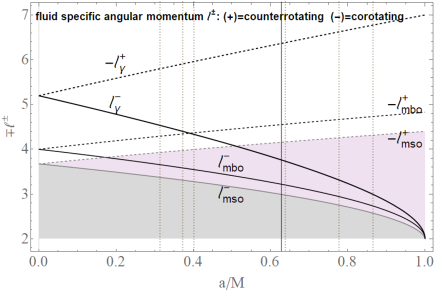
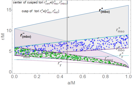
Figure 2: Upper panel: Fluid specific angular momentum $\ell^{\pm}$ of the tori in the RAD, for corotating $(-)$, and counterrotating $(+)$, fluids, versus SMBH dimensionless spin $a/M$. The tori are for $\mp\ell^{\pm}>\mp\ell_{mso}^{\pm}$ respectively. There is $\ell_{\bullet}\equiv\ell(r_{\bullet})$ for $r_{\bullet}=\{r_{mso},r_{mbo},{r_{\gamma}}\}$, $r_{mso}$ is the marginally stable circular orbit, $r_{mbo}$ is the marginally bounded orbit and $r_{\gamma}$ the last circular (photon) orbit. Bottom panel: radii $r_{mbo}$ and $r_{mso}$ and the pair $r_{(mbo)}$ and $r_{(mso)}$ defined in Eq. (29) as functions of the dimensionless spin of the BH. Regions of Table (1) are shown.

respectively for the counterrotating $(+)$ and corotating $(-)$ orbits. This expanded geodesic structure, represented by the union of radii $R$ and $R_{(r)}$ sets, rules large part of the geometrically thick disk physics and multiple structures in the RAD model. The presence of these radii stands as one of the main effects of the presence of a strong curvature of the background geometry(Pugliese&Stuchlik, 2018a, 2016, b). In Table (1) we summarize the constraints, defining ranges of fluids specific angular momentum $(\mathbf{L_{1},L_{2},L_{3}})$, see also Figs (2).

[$\ell\in\mathbf{L_{1}}$: quiescent and cusped tori]–$\mp\mathbf{L_{1}}^{\pm}\equiv[\mp\ell_{mso}^{\pm},\mp\ell_{mbo}^{\pm}[$:
topologies $(C_{1},C_{\times})$; accretion point $r_{\times}\in]r_{mbo},r_{mso}]$ and center with maximum pressure $r_{cent}\in]r_{mso},r_{(mbo)}]$;
[$\ell\in\mathbf{L_{2}}$: quiescent tori and proto-jets]–$\mp\mathbf{L_{2}}^{\pm}\equiv[\mp\ell_{mbo}^{\pm},\mp\ell_{\gamma}^{\pm}[$:
topologies $(C_{2},O_{\times})$ are possible; unstable point $r_{j}\in]r_{\gamma},r_{mbo}]$ and center with maximum pressure $r_{cent}\in]r_{(mbo)},r_{(\gamma)}]$;
[$\ell\in\mathbf{L_{3}}$: quiescent tori] $\equiv\mp\mathbf{L_{3}}^{\pm}\equiv\ \ell\geq\mp\ell_{\gamma}^{\pm}$:
quiescent torus $C_{3}$ with center $r_{cent}>r_{(\gamma)}$;

Table 1: It is $mso$ for marginally stable orbit and $mbo$ for marginally bounded orbit, $\gamma$ is for marginally circular orbit (photon orbit)–see also Eq. (29) for details on notation and Figs (2) for the representation of the different regions.

These models allow the determination of a wide number of aspects of disks morphology, dynamics and stability. Although restricted by the typical assumptions of these simplified models, thick (stationary) disks provide a striking good approximation of several aspects of accretion instabilities in different and more refined dynamical models. Some of these features are the tori elongation on their symmetry plane, the inner edge of quiescent and accreting disks, the tori thickness, the maximum height, and the critical pressure points. It is possible to evaluate for example the inner and outer edge of an accretion torus as follows:

$$r_{in}(a;\ell,\overline{Q})=-\frac{2}{3}\left[\mathbf{\alpha}\cos\left[\frac{1}{3}(\pi+\arccos\beta)\right]+\frac{1}{\overline{Q}}\right],$$ (31)

$$r_{out}(a;\ell,\overline{Q})=\frac{2}{3}\left[\alpha\cos\left(\frac{1}{3}\arccos\beta\right)-\frac{1}{\overline{Q}}\right],$$ (32)

$$\mbox{where }\quad\alpha=\sqrt{\frac{4+3\overline{Q}\left[(\overline{Q}+1)(\ell^{2}-a^{2})+a^{2}\right]}{\overline{Q}^{2}}},\quad\overline{Q}\equiv(K^{2}-1)<0,$$

$$\beta=-\frac{9\overline{Q}\left[(\overline{Q}+1)(\ell^{2}-a^{2})+a^{2}\right]+8+27(\overline{Q}+1)\overline{Q}^{2}(a-\ell)^{2}}{\alpha^{3}\overline{Q}^{3}}$$ (33)

(dimensionless units have been used). The use of notation (i): $\textbf{()}_{i}^{\pm}<\textbf{()}_{o}^{\pm}$ and (ii): $\textbf{()}_{i}^{\pm}<\textbf{()}_{o}^{\mp}$, for a tori couple in a eRAD highlights some properties of these structures. Using the couple seeds for the two eRAD configurations in notation (i) for a $\ell$corotating and (ii) and a $\ell$counterotating couple, one can characterize different phases of possible eRAD evolution. Also, symbols $\lessgtr$ $\left(\lessgtr_{\mathbf{\times}}\right)$ for two tori refer to the relative position of the tori centers $r_{cent}$ (accretion points or unstable points $r_{\times})$: thus, for example, we use short notation $(\textbf{()}^{-}<\textbf{()}^{+},\textbf{()}^{-}<_{\mathbf{\times}}\textbf{()}^{+})\equiv\textbf{()}^{-}\ll_{\mathbf{\times}}\textbf{()}^{+}$ that means $r_{cent}^{-}<r_{cent}^{+}$ and $r_{\times}^{-}<r_{\times}^{+}$. In the eRAD the seed couple introduced in Pugliese&Stuchlik (2017a) is in fact a pair of tori, intended as constructive seed as it serves from the methodological viewpoint to manage the constraints on the effective potential of the entire eRAD structure introduced in Pugliese&Stuchlik (2015) and more generally to study the entire structure as a whole orbiting body with a complex and diversified intern. Conversely, the introduction of a law of rotation as the leading function for eRAD and RAD is intended as the distribution of the points of maximum pressure and minimum pressure in a generic distribution of extended orbiting matter with some symmetries - it should then be understood that it must be specified how to consider properly an extended matter structure in the sense of this rotational law. Each point in the stability area of the leading function, that is to the right $r>r_{mso}^{\pm}$of the discriminant radius $r_{mso}^{\pm}$ (a minimum of $\pm\ell^{\mp}(r)$), respectively for the two directions of rotation, has to be understood as pressure/density seeds for toroidal rings growing. The regions for corotating and counterrotating fluids are superimposed depending on the spin value $a/M$. According to different ranges of $a/M$ values, there are several aggregation structures seeds of super-Keplerian matter in the sense of $|\ell|\geq|L|$, this makes the analysis of the eRAD complex but also provides a surprisingly refined method to obtain restricted constraints for the RAD-SMBH systems. (We specify that here as elsewhere the term Keplerian refers in short to the motion of a free particle located on circular orbit around.). This is mainly due to the fact that orbital regions with boundary defined by the intersection of the radial ranges from the $R$ and $R_{(r)}$ sets with the additional couple $(r_{\mathcal{M}},r_{(\mathcal{M})})$ strongly depend on the dimensionless spin of the attractor especially for the $\ell$corotating couples, with an even more complex structure for the $\ell$corotating tori sequences composite of corotating tori. Furthermore there is the addition complication, for the orbiting multi-structures, due to the fact that corotating and counterrotating structures must be considered together, substantially coupling the two separated analysis with further combinations of finite but complex constraints– Pugliese&Stuchlik (2017a, 2019, 2018a). We show an aspect of this condition below by providing an example of the limits imposed on the attractor spin. In this context, the radii $r_{(\mathcal{M})}$ in the unstable region and $r_{\mathcal{M}}>r_{mso}$ in the stability region, must also be interpreted as extreme in the distribution of seeds of tori (the stability points) and instability points (obviously corresponding to the left range $r<r_{mso}^{\pm}$). These are interpreted as the maximum of distributions of points of the aggregation seeds in accordance with the maximum and minimum points of pressure. It can be shown that these radii are related to the derivatives of certain frequencies of oscillations typical of thick toroidal structures (Pugliese&Montani, 2018d). According to different conditions set on the RAD, there are further limits to the inequality $|L|<|\ell|$. Accordingly, for example, there are the following critical values of the spin:

$$a_{1}\equiv 0.4740M:\quad r_{(mbo)}^{+}=r_{({{\gamma}})}^{-},\quad a_{2}=0.461854M:\;r_{(mbo)}^{-}=r_{mso}^{+}$$

$$a_{3}\equiv 0.73688M:\;r_{({\gamma})}^{-}=r_{\mathrm{mso}}^{+},$$ (34)

These identify, on the basis of the doubled geodesic structures classes of attractors where specific eRAD can be observed (Pugliese&Stuchlik, 2018a).

3.4 Multi-accretion processes, multi–orbiting structures and ringed accretion disks

The RAD structures pose the interesting issue of the internal activity of the tori ringed cluster and particularly the internal exchanges of energy and matter between the tori and the tori and central SMBH. In this respect, eRAD system, RAD and globuli are characterized by a vivid internal activity made up of collision among tori, inner accretion, internal jet launching, whether constrained by open-proto-jet configurations considered here, in conjunction with an inner edge-accretion jet emission correlation. These structures can also constitute a basis for interpretation of the mass accretion rates of supermassive black holes in AGNs, and several other phenomena connected with energetics of the accretion disks, but also the evolution of the central attractor with particular respect to its spin evolutions. The RADs model follows the possibility that more accretion orbiting configurations can form around very compact objects in the special environment of the AGNs-BHs and Quasars. Arising from different BHs accretion periods and from the host Galaxy life, such configurations can report, in their characteristics, traces of the different periods during several accretion regimes occurred in the lifetime typical of non-isolated Kerr BHs (Alig et al., 2013; Blanchard et al., 2017; Pugliese&Stuchlik, 2018b; Nixon et al., 2012). During the evolution of BHs in these environments both corotating and counterrotating accretion stages are mixed during various accretion periods of the attractor life (Lovelace&Chou, 1996; Carmona-Loaiza et al., 2015; Dyda et al., 2015; Volonteri et al., 2003a), thus RADs tori may be even misaligned (Aly et al., 2015). An example of eRAD composed by three tori is in Fig (1). These systems, including accretion disks misaligned with respect to the spin of a central black hole, formed in AGNs, may be consequential to periods of chaotical accretion, where corotating and counterrotating tori and strongly misaligned disks can be formed.

Misaligned disks have been studied for example in King&Nixon (2018); Aly et al. (2015); Nixon et al. (2012); Kovar et al. (2011); Slany et al. (2013); Kovar et al. (2014); Kovár et al. (2016); Trova et al. (2018c). However, in the context of the misaligned tori, a Kerr black hole plays a relevant role both in the disk structure and for the effects that the disk evolution has on the evolution of the central BH spin. In the context of the misaligned tori, a BH warped torus evolves together with its attractor changing its mass, the magnitude of its spin, and the spin orientation. The impact of the BHs spin on the misaligned disks merges with the complexity of a RAD structure reflecting in the Bardeen-Petterson effect, causing shift of the tilted accretion disk into the BH equatorial plane due to the combined effect of the disk inclination and the frame dragging of the Kerr spacetime (Bardeen&Petterson, 1975). RAD structures are governed mainly by geometry of the Kerr SMBH attractors– Pugliese&Stuchlik (2015, 2016, 2017a, 2018c, 2018b, 2019); Pugliese et al. (2013); Pugliese&Montani (2018d); Pugliese&Stuchlik (2018a). In the eRAD a tori couple (a state) with only the inner accreting (cusped) torus and an outer accreting counterrotating configuration is possible, keeping the stability of the RAD structure. The misalignment of the toroidal structures allows to reconsider in some extent the possibility of the presence of multi accreting tori on different planes, enlightening interesting situations and phenomenologies which were not allowed for the eRAD. There is the possibility that the presence of more accreting RAD tori (including collisional regions) could increase the accretion rate of the central BH.

In the RAD composed by misaligned tori it has been explored the hypothesis of a quasi-complete covering of the BH horizon with a BH embedded in a accreting ball made by a composition of RAD tori having different orientations of the fluids specific angular momentum (tori spins). In the RAD context, under special conditions (depending on number of toroidal components and tori geometrical thickness), the system of BH entangled tori could be considered as a matter embedding, covering the central BH from a distant observer at different angles. A globus of clustered tori is constituted by a multipoles orbiting matter embedding surrounding the central BH converging the BH horizon. These globuli, being constituted by orbiting matter with different spin orientations constitute in this sense a multipole orbiting configuration with a central BH object that may have significant role in different epochs of the BH life.

RAD phenomenology

RADs Instabilities may reveal therefore of significance for the High–Energy Astrophysics related especially to accretion onto supermassive BHs, and the extremely energetic phenomena occurring in Quasars and AGNs that could be observable by the X-ray observatory ATHENA. From the phenomenological viewpoint, the RAD model constitutes a shift in paradigma from the interpretative framework of the BH-disk interaction to the BH-RAD and clearly opens a broad scenario of investigation. The RAD model opens the possibility to review the main template of analysis from a SMBH-disk framework to a SMBH-RAD one. The eRAD is constructed as a whole, geometrically thin disk. The current interpretative framework of the BH-accretion disk physics generally foresees the scenario of a BH-one disk system, implying therefore the possibility of a “RAD in disguise”, i.e. a RAD could be observed as a geometrically thin, axis-symmetric disk, centered on the equatorial plane on a Kerr SMBH, with a “knobby” surface and characterized by a differential rotation with peculiar optical properties, particularly the X-ray emission is expected to show the ringed structure in a discrete emission profile. In this respect we can consider the analysis in Sochora et al. (2011); Karas&Sochora (2010); Schee&Stuchlik (2009, 2013) where relatively indistinct excesses of the relativistically broadened emission-line components were predicted arising in a well-confined radial distance in the accretion structure, supposed to be originated by a series of episodic accretion events. More generally the AGN X–ray variability suggests connection between X-rays and the innermost regions of accretion disk. This makes reasonable to reinterpret the observations analyzed so far in the single-torus framework, in a new interpretive frame represented by the possibility of a multi-tori system. RAD are characterized by peculiar phenomena associated to the instabilities, as the occurrence of double accretion and its after-dynamics, the inter disks proto-jet emission and the screening tori. Instabilities should be treated in accordance with a global point of view where the macrostructure is considered as a single, unique disk orbiting around a central SMBH. For example the radially oscillating tori of the couple could be related to the high-frequency quasi periodic oscillations observed in non-thermal X-ray emission from compact objects. These emissions could be interpreted as fingerprints of the characteristic discrete radial profile of the ringed structure.

Notes on the RAD instabilities We conclude this section with further comments on the stability of the RADs configurations. It is clear that the instability of each RAD component must reflect in an inter-RAD disk activity. More in general, there are different RAD instabilities. A destabilization of the system structure may arise after the emergence of an instable phase of one component of the RAD, for example after an accretion phase of one torus onto the central BH or the proto-jet emission which is capable to destabilize the entire disk Pugliese&Stuchlik (2018b, c). This case however has been strongly constrained. The maximum number of accreting tori in a eRAD is $n_{\times}=2$, occurring for the couple $\mathrm{C}_{\times}^{-}<\mathrm{C}_{\times}^{+}$, made by an inner corotating and an outer counterrotating torus accreting on the BH. Secondly a RAD can be destabilized after collision of a pair of quiescent tori of the agglomeration. Collision may arise for example after growing of one torus (Pugliese&Stuchlik, 2017a, 2019). In the couple $\textbf{()}^{-}<\mathrm{C}_{\times}^{+}$, the accretion phase of the outer torus and the collision emergence can combine establishing a complex phase of RAD destabilization. The particular case of the emergence of collision for two RAD tori was considered in Pugliese&Stuchlik (2017a), while interacting tori and energetic of associated to these processes were investigated in Pugliese&Stuchlik (2019). The mass accretion rates, the luminosity at the cusps and other fundamental characteristics of the BHs accretion disk physics were also evaluated. In Pugliese&Stuchlik (2015), RAD perturbative approaches have also been described, in Pugliese&Stuchlik (2016), the emergence of unstable tori have been detailed, while further discussion on RADs as remnants of AGN accretion periods are in Pugliese&Stuchlik (2018b).

A further interesting case is the sequence of three configurations $\textbf{()}^{-}<\mathrm{C}_{\times}^{+}<\mathrm{C}^{\pm}$ which is a system where the inner, accreting or quiescent, torus can be an obscuring inner torus. Matter, from the outer counterrotating torus, impacts on the corotating inner one, which is screening the accretion from the central SMBH. Collision however may give rise to several possibilities. A possibility consists in the formation of in a single torus, in fact canceling the RAD structure. This is a phenomenon which may affect mainly the first evolution phases of the formation of the aggregate. An inner torus of the orbiting RAD couple may form as axially symmetric corotating toroidal disk after a first phase of formation of the outer aggregate component. Another possibility is the occurrence of a “drying-feeding” phase, involving interrupted stages of accretion of one or two tori of a couple: matter flows between the two tori of the couple give raise to a series of interrupted stages of accretion onto the central SMBH. This particular effect, considered in Pugliese&Stuchlik (2017a, 2018b) and detailed in Pugliese&Stuchlik (2019) can model the different phases of super-Eddington accretion advocated as a mechanism to explain the large masses observed in SMBHs at high redshift–see for example Volonteri et al. (2007); Volonteri (2007, 2010); Li (2012); Oka et al. (2017); Kawakatu&Ohsuga (2011); Allen et al. (2006). It is however necessary to consider the oscillations and instabilities associated with the each component of the aggregate–eventually this can be also related to QPOs emission–see Montero et al. (2007). More precisely, the collision instability can lead to different evolutive paths for the aggregate tori, depending on the initial conditions of the processes as the torus rotation with respect to the black hole, the range of variation of the mass of the torus and of the magnitude of the specific angular momentum of the fluids. We also mention the case of the runaway-runaway instability which is a combination of runway instability and collision of the inner disk with the outer configuration or, as analyzed in Pugliese&Stuchlik (2018a), the combination of chaotic effects induced in the accretion rate. A further important features of thick disks is the Papaloizou-Pringle (PP) global incompressible modes and the Papaloizou-Pringle Instability (PPI), which is the global, hydrodynamic, non-axis-symmetric instability which can combine eventually with parallel emerging Magneto-Rotational Instability modes. In the geometrically HD thick disks, the accretion process is strictly interwoven with the development of the PP instability: the mass loss in the Roche lobe overflow regulates the accretion rate in the innermost part of torus. This self-regulated process on one side locally stabilizes the accreting torus from the thermal and viscous instabilities and, on the other side, it globally stabilizes the torus from the PPI. As mentioned above, in these disks, the PPI hydrodynamic instability can entangle with an emerging MRI which triggers eventually predominant larger modes of oscillation (smaller length scales) with respect to typical PPI modes, and creating a far richer and complex scenarios for the torus equilibrium properties. (Note also that the amount of overflow may be also modulated by global disks oscillations). On the other hand, the Papaloizou-Pringle (global and non-axis-symmetric) Instability is able to transport angular momentum outwardly in the disk and therefore able to finally trigger the accretion . In this respect we should note that global instabilities are affected by the boundary conditions assumed for the system. In the case of PPI in RAD accreting HD tori, for which the disk inner and outer edges are well defined, the PPI is generally suppressed, stabilizing the disks by the accretion flow driven by the pressure forces across the cusp, $r_{\times}$. The relative importance of MRI and PPI and the interaction of two processes depends in fact on many factors and conditions. In particular in the RAD scenario different factors can be determinant: the (turbolent) resistivity, the emerging of a dynamo effect, the study for counterrotating (retrograde) tori, the disk self-gravity, the gravitational interaction between the disk and the central Kerr SMBH and the runaway instability are further aspects which may contribute importantly to the characterization of the ongoing processes. In Sec. (4), we investigate the magnetized tori endowed with a toroidal magnetic field, grounded on the HD models investigated here.

4 Magnetized tori: toroidal magnetic field in multi-accreting tori

In Pugliese&Montani (2013a, 2018d) RADs framework has been used to investigate the influence of the magnetic field in the formation of the torus, as a limiting case of the eRADs and hence in the formation of the multiple accreting events occurring around a Schwarzschild and Kerr SMBH. Differences between the magnetize case and the HD models, are particularly evident in the unstable phases due to the tori collision and the accretion. In this section we consider RAD with toroidal sub-structures regulated by the presence, in the force balance equation, of a toroidal magnetic field component. We refer to the analysis of Pugliese&Montani (2018d, 2013a). The toroidal magnetic field form used here is the well known Komissarov-solution (Komissarov, 2006), used in the approach (Pugliese&Montani, 2013a, 2018d; Pugliese&Stuchlik, 2020c), see also Abramowicz&Fragile (2013); Porth et al. (2017); Pugliese&Montani (2013a); Adamek&Stuchlik (2013); Hamersky&Karas (2013); Karas et al. (2014); Slany et al. (2013); Kovar et al. (2011); Fragile&Sadowski (2017); Gimeno-Soler&Font (2017). This is a well known solution of toroidal magnetic field widely adopted in the axis-symmetric accretion configurations. The magnetized torus of RAD is widely used to fix up the initial configurations for numerical integration of a broad variety of GR-MHD models. In our application here we generalize this approach to the discussion of thick disks and their morphology reflected by the presence of magnetic field and secondly the analysis of angular momentum distribution in the aggregate context of eRAD. More precisely in this section we consider axially symmetric spacetimes as Kerr or the static limit of the Schwarzschild exact solutions. We also mention Zanotti&Pugliese (2014) for a discussion on the case of a poloidal magnetic field where a metric representation is adapted to the direction of the field, as proved by Bekenstein&Oron (1978, 1979). This work comments on the application and role of von Zeipel theorem for this particular case of introduction of poloidal magnetic field. The choice of a purely azimuthal (toroidal) magnetic field is particularly adapted to the disks symmetries considered here and largely adopted as initial setup for numerical simulations in several general relativistic magnetohydrodynamic models sharing similar symmetries with the RAD and thick disks considered here(Porth et al., 2017).

Magnetic field can have a major influence in the BH-accretion disk systems, especially during the early stage of tori formation and the final steps of evolutions towards the accretion onto the spinning BH, a phase where predominant instabilities occur for the accreting torus as well as for the RAD system. The tori rotational law (specific angular momentum) is therefore expected to depend on the magnetic field. The counterrotating and $\ell$counterrotating cases are proved significantly that the toroidal magnetic field plays an essential role in determining the disk structure and stability, showing that also a purely azimuthal field is capable to discriminate the eRAD features.

One question faced in Pugliese&Montani (2013a) is if thickness of a toroidal accretion disk spinning around a Schwarzschild or Kerr Black hole can be effected under the influence of a toroidal magnetic field and by varying the fluid angular momentum. In the HD case, where there is only a centrifugal component originated by the fluid rotation or eventually the dragging of the central attractor, the torus thickness remains basically unaffected but tends to increase or decrease slightly depending on the gravitational and centrifugal effects which the disk is subjected to. In Pugliese&Montani (2013a) it is addressed for example the specific question of torus squeezing on the equatorial planes of the central attractor, exploring the disk thickness changing the physical characteristics of the torus as the angular momentum and the effective potential which characterize the toroidal surface. From the methodological viewpoint, the magnetic field contribution has been then considered as part of the exact GR effective potential functions. This analysis focuses on role that a toroidal field could have in determining the morphology when considered as part of the pressure and modification of effective potential according to the model developed in Sec. (3). Moreover a consequent problem consists in questioning the role that a toroidal magnetic field could play as a contributing factor to the collimation or launch of a jet matter component along disk and BH rotation axis —(Pugliese&Stuchlik, 2018c).

The second issue addressed in this section is a brief discussion on the angular momentum distribution and part of the stability analysis in the eRAD agglomerate. In Pugliese&Montani (2018d) it is analyzed the effects of a toroidal magnetic field in the formation of several magnetized accretion tori orbiting around one central Kerr SMBH in AGNs, where both corotating and counterotating disks are considered on its equatorial plane, while the analysis of RAD misaligned in globular form around a static attractor is developed in Pugliese&Stuchlik (2020a). This analysis leads therefore to constrain tori formation and emergence of RADs instabilities, accretion onto the central attractor and tori collision emergence, are investigated. Concerning the instability it is convenient to remind here that geometrically thick disks are subjected to several oscillation modes. One modes set is constituted by incompressible and axis-symmetric modes corresponding to global oscillations for radial, vertical and epicyclic frequencies together with surface gravity, acoustic and internal modes which are recovered from the so called relativistic Papaloizou-Pringle (PP) equation–(Abramowicz&Fragile, 2013). The introduction of a purely toroidal and even small magnetic field (considering the magnetic pressure versus gas pressure as defined by the $\beta$-parameter) can have influence on the development of these modes. This is relevant particular for the torus global non-axis-symmetric modes, because of the generation of the Magneto-Rotational Instability due to the magnetic field and fluid differential rotation. The presence of a magnetic field contribution in the disk force balance leads to a more complex situation where the PPI has to be considered in a broader context. More generally, whether or not the hydrodynamical oscillation modes in MHD geometrically thick disks may survive such global instabilities or the presence of a weak magnetic field would strongly affects these, is still under investigation. The linear development of the PPI can however be affected by the presence of a magnetic field and by a combined growth of the MRI. These two processes can coexist, enter into competition or combine depending on local parameters of the model (strongness of the magnetic field as evaluated by $\beta$ parameter). Some studies seem to suggest that under certain conditions on the strength of the magnetic field and other conditions on the torus onset, this situation can also be resolved in the PPI suppression by the MRI in the relativistic accretion disks.

In the case of geometrically thick torus endowed with a (purely) toroidal magnetic field, considered here with the analytic Komissarov solution, a series of recent analysis shows that torus is violently prone to develop the non-axisymmetric MRI in 3D which could disturb this configuration on dynamical timescales–see (Del Zanna et al., 2007; Wielgus et al., 2015; Das et al., 2017) and (Bugli et al., 2018). In the magnetized tori, as the RAD tori considered in this section, the accretion is triggered at much earlier times then in the HD tori, and modes higher then the azimuthal $m=1$ mode, typical of HD-PPI tori, emerge together with $m=1$. GR-MHD investigations show generally an increase of turbulent kinetic energy in the earlier phases competing with the GR-HD ones, consequently accretion is in fact triggered by the Maxwell stresses instead of the PPI. Eventually the fundamental mechanism responsible for the onset of the PPI does not appear to be the predominant one or even to arise at all in the MHD torus. In the magnetized case on the other hand there is a broader range of excited frequencies with respect to the GR-HD model. In general recent analysis show that the inclusion of a toroidal magnetic field could strongly affect, even with a sub-thermal magnetic field, the PPI (there are suggestions that the action of MRI suppresses the PPI $m=1$ mode growth). This may have a relevant consequence in the double RAD system as MRI stabilizes the disks to PPI with MHD turbulence. The evaluation of the accretion rates in the GR-HD double RAD systems has been carried out in Pugliese&Stuchlik (2019). It appears however that MRI is more effective and faster in transport of angular momentum across the disk, and higher accretion rates were proved to occur in the magnetized models. Finally it should be noted that, according to Fragile&Sadowski (2017), strong toroidal magnetic fields are rapidly suppressed in this tori, in favor of weaker fields (decrease of $\beta$ parameter).

In the following we first set the problem writing the main equations and discussing leading function for the tori distributions in the eRAD agglomeration. Then considerations on magnetic fields and the choice of the magnetic parameters values follow. The section closes with some considerations on aspects of the magnetize disks morphology and stability. In this section we use mainly dimensionless units.

Set-up review

As noted in Komissarov (2006) the presence of a magnetic field with a relevant toroidal component can be related to the disk differential rotation, viewed as a generating mechanism of the magnetic field, for further discussion we refer to Komissarov (2006); Montero et al. (2007); Parker (1955, 1970); Yoshizawa et al. (2003); R-ReS1999, while we refer to Pugliese&Montani (2013a); Adamek&Stuchlik (2013); Hamersky&Karas (2013); Karas et al. (2014); Abramowicz&Fragile (2013) where this solution is dealt in detail in the context of accretion disks. In the magnetized case, following (Pugliese&Montani, 2013a, 2018d), therefore we consider an infinitely conductive plasma where $F_{ab}U^{a}=0$, where $U^{a}B_{a}=0$, with $\partial_{\phi}B^{a}=0$ and $B^{r}=B^{\theta}=0$. We obtain the relation $B^{t}=U^{\phi}B^{\phi}/U^{t}=\Omega B^{\phi}$ . We can write the Euler equation (18) as

$$\frac{\partial_{*}p}{\rho+p} = G_{*}^{(f)}+G_{*}^{(em)},\quad G_{*}^{\natural}=-\frac{\partial}{\partial*}W^{\natural}_{*}\quad\mbox{where}\quad W_{*}^{f}\equiv\ln V_{eff},,$$ (36)

$$W_{*}^{(em)}\equiv G_{*}(r,\theta)+g_{*}(\theta),\quad*=\{r,\theta\},\quad\natural=\{(em),(f)\}$$

where $g_{\theta}(r)$ and $g_{r}(\theta)$ are functions to be fixed by the integration. Within particular conditions on the fields the general integral is

$$\int\frac{dp}{\rho+p}=-(W^{(f)}+W^{(em)}).$$ (37)

The Euler equation for this system has been exactly integrated for the background spacetime of Schwarzschild and Kerr BHs in (Komissarov, 2006; Montero et al., 2007) with a magnetic field is

$$B^{\phi}=\sqrt{\frac{2p_{B}}{g_{\phi\phi}+2\ell g_{t\phi}+\ell^{2}g_{tt}}}\quad\mbox{or alternatively},$$ (38)

$$B^{\phi}=\sqrt{{2\mathcal{M}\omega^{q}}}\left(g_{t\phi}g_{t\phi}-g_{{tt}}g_{\phi\phi}\right){}^{(q-2)/2}V_{eff}(\ell)$$ (39)

where $p_{B}=\mathcal{M}\left(g_{t\phi}g_{t\phi}-g_{{tt}}g_{\phi\phi}\right){}^{q-1}\omega^{q}$ is the magnetic pressure, $\omega$ is here the fluid enthalpy, $q$ and $\mathcal{M}$ are constant. (For $q\neq 1$ it is $G_{r}(r,\theta)=G_{\theta}(r,\theta)=G(r,\theta),$ in Eq. (36)). We assume moreover a barotropic equation of state. According to our set-up we introduce a deformed (magnetized) Paczyński potential function and the Euler equation (36) becomes:

$$\partial_{a}\tilde{W}=\partial_{a}\left[\ln V_{eff}+G\right]\,\mbox{where}$$ (40)

$$(a\neq 0):G(r,\theta)=\mathcal{S}\left(\mathcal{A}V_{eff}^{2}\right)^{q-1}=\mathcal{S}\left(g_{{t\phi}}g_{t\phi}-g_{tt}g_{\phi\phi}\right)^{q-1};$$ (41)

$$\mbox{and}\;\mathcal{A}\equiv\ell^{2}g_{tt}+2\ell g_{t\phi}+g_{\phi\phi},\quad\mathcal{S}\equiv\frac{q\mathcal{M}\omega^{q-1}}{q-1}$$

$\mathcal{S}$ is a magnetic parameter, $q$ and $\mathcal{M}$ (magnitude) are constant . We therefore consider the equation for the $\tilde{W}=$constant. The toroidal surfaces, obtained from the equipotential surfaces (Boyer, 1965; Pugliese&Montani, 2013a), are provided considering this function

$$\widetilde{V}_{eff}^{2}\equiv V_{eff}^{2}e^{2\mathcal{S}\left(\mathcal{A}V_{eff}^{2}\right){}^{q-1}}=$$ (43)

$$\frac{\left(g_{t\phi}g_{t\phi}-g_{tt}g_{\phi\phi}\right)\exp\left(2S\left(g_{t\phi}g_{t\phi}-g_{tt}g_{\phi\phi}\right)^{q-1}\right)}{\ell^{2}g_{tt}+2\ell g_{t\phi}+g_{\phi\phi}}=K^{2}.$$

Potential $\widetilde{V}_{eff}^{2}$, for $\mathcal{S}=0$ reduces to the effective potential ${V}_{eff}^{2}$ for the non-magnetized case $V_{eff}$, a function of the metric and the angular momentum $\ell$. The torus shape is determined by the equipotential surfaces which now are regulated in eq. (37) by an effective potential deformed, respect to the HD case ($B=0$), by the magnetic field. (We note here that, the magnetic pressure is regarded as a perturbation of the hydrodynamic component, it is assumed that the Boyer theory remains valid and applicable in this approximation –discussions on similar assumptions can be found in Komissarov (2006); Abramowicz&Fragile (2013)).

Leading function: tori distribution law

As for the HD case, we could find the RAD angular momentum distribution:

$$\widetilde{\ell}^{\mp}\equiv\frac{\Delta\left(a^{3}+ar\left[4\mathcal{Q}(r-M)\mathcal{S}\Delta^{\mathcal{Q}}+3r-4\right]\mp\sqrt{r^{3}\left[\Delta^{2}+4\mathcal{Q}^{2}(r-1)^{2}r\mathcal{S}^{2}\Delta^{2\mathcal{Q}+1}+2\mathcal{Q}(r-1)^{2}r\mathcal{S}\Delta^{\mathcal{Q}+1}\right]}\right)}{a^{4}-a^{2}(r-3)(r-2)r-(r-2)r\left[2\mathcal{Q}(r-1)\mathcal{S}\Delta^{\mathcal{Q}+1}+(r-2)^{2}r\right]}$$

$$\mbox{where there is }\,\lim_{\mathcal{\mathcal{S}}\rightarrow 0}\widetilde{\ell}^{\mp}=\lim_{q\rightarrow 1}\widetilde{\ell}^{\mp}=\ell^{\pm},\quad\mathcal{Q}\equiv q-1$$ (44)

or alternatively

$$\quad\mathcal{\mathcal{S}}_{crit}\equiv-\frac{\Delta^{-\mathcal{Q}}}{\mathcal{Q}}\frac{a^{2}(a-\ell)^{2}+2r^{2}(a-\ell)(a-2\ell)-4r(a-\ell)^{2}-\ell^{2}r^{3}+r^{4}}{2r(r-1)\left[r(a^{2}-\ell^{2})+2(a-\ell)^{2}+r^{3}\right]}$$ (45)

(dimensionless units)–(Pugliese&Montani, 2018d). We provided two different tori distribution laws. In fact, as noted in Pugliese&Montani (2018d) the introduction of a toroidal magnetic field $B$, makes the study of the momentum distribution within the disk rather complicated. In Pugliese&Montani (2018d) the critical function $\mathcal{S}_{crit}$ has been introduced as alternative to represent, instead of $\tilde{\ell}$, the new leading function for the distribution of tori in the RAD having a toroidal magnetic field component (each torus is on a line $\mathcal{S}=$constant with $\ell=$constant value) and able to determine the limits on the value of the magnetic parameter for the tori formation, the emergence of HD instability associated with the cusped configurations, $\mathrm{C}_{\times}$ and $O_{\times}$, and the emergence of collision between two tori of a RAD couple. This function, derived from $\mathcal{S}$-RAD parameter, is capable of setting the location of maximum density points in the disk and the existence and location of the instability points.

The advantage in using this particular distribution, not directly connected to the specific momentum distribution of the matter in orbiting rings, is that it highlights the difference between magnetized corotating and counterrotating tori with respect to the central BH rotation, which is not immediate with the distribution of momentum $\tilde{\ell}$. The function $\mathcal{S}_{crit}$ clearly enucleates the magnetic field contribution in the $\mathcal{Q}$ term, while interestingly highlights the role of the parameters $\ell$ versus $a$–(Pugliese&Stuchlik, 2018c). (We also note the dependence from the quantities $(a\pm\ell)$ which directly connects the specific spin of the central attractor in the limits $a\in[0,M]$ with the momentum of the fluid. In suitable conditions on the distance of the orbiting fluid from the central attractor and the configurations symmetries, the ratio $a$ versus $\ell\sqrt{\sigma}$ or $\ell$ versus $a/\sqrt{\sigma}$ are considered).

As demonstrated in Pugliese&Montani (2018d), the magnetized tori can be formed in the eRAD agglomerates for sufficiently small $(q\mathcal{S})$. The constraints described in Sec. (3.3) are essentially confirmed for the magnetized case even when the pressure force induces a modification of the effective potential governing the fluid. Profiles of $\ell$corotating tori distributions are similar independently by the corotation or counterrotation of the fluids in the eRAD with the respect to the central Kerr SMBH. Generally the inner torus has maximum values of the $\mathcal{S}$ smaller then the maximum of $\mathcal{S}$ found in the outer tori. The most interesting results emerge in the case of $\ell$countorrotating couples where it is clear that the magnetic profiles for a couple $C_{-}<C_{+}$, constituting, according to notation of Sec. (3.3) by a couple of inner corotating torus and outer counterrotating torus, where double accretion occurs, are radically different from the case $C_{+}<C_{-}$ (inner counterrotating and outer corotating torus). The analysis shows also the importance of the coupling between the toroidal component of the magnetic field and the fluid angular momentum, particularly in the counterrotating case, $\ell<0$, for values $q<1$ when excretion can arise.

Consideration on magnetic fields and choice of parameters: extended range of field parameters.

Some values of $\mathcal{Q}\equiv q-1$ (dimensionless units) in $\mathcal{S}_{crit}$ may also provide for excretion disks implying configurations with minimum (unstable points) of pressure far from the stability points in the momentum distribution and far from the attractor, and with extreme conditions on the magnetic term. These situations are otherwise typical of special scenarios with a resulting "repulsive" force, due to the presence of electrically charged fluids (Kovar et al., 2011; Trova et al., 2016, 2018b; Kovár et al., 2016; Kovar et al., 2014; Slany et al., 2013; Trova et al., 2018c), a naked singularity background (Adamek&Stuchlik, 2013; Stuchlik&Schee, 2013; Stuchlik& Schee, 2010; Stuchlik et al., 2011) or a particular cosmological scenario (Stuchlik, 2005; Stuchlik et al., 2009; Slaný&Stuchlík, 2005; Stuchlik&Kovar, 2008), or also emerging from hints of the deep structure of some geometry modifications due to quantum effects resulting in the repulsive force observable, on the large scales of these agglomerates, as engines empowering the excretion tori (Stuchlik et al., 2015). The range of this parameter is clearly divided into three regions: (i) $q>1$, with a subrange (ii) with extreme $q=2$; (iii) $0<q<1$. (i)For $q>1$ we get closed surfaces in the limit $\mathcal{S}\approx 0$, which is in agreement with expansion around $\mathcal{S}=0$, that is, when the contribution of the magnetic pressure to the torus dynamics is properly regarded as a perturbation with respect to the hydrodynamics solution. This is realized when an appropriate condition $(\mathcal{S}\ll 1)$ on the field parameters is satisfied. The general trend of $\mathcal{S}_{crit}$ as function of $r$ is as follows: there is a maximum such that $\mathcal{S}_{crit}\in[0,\mathcal{S}_{\max}]$, that is $\mathcal{S}$ is bounded below by the non-magnetized case and above by a maximum value $\mathcal{S}_{\max}$. (It can be shown that the maximum value $\mathcal{S}_{\max}$ depends linearly on $q$.). The presence of a maximum value is however not always satisfied, depending mostly on the relative rotation of the fluids and also from the BH spin. (ii)The case $q=2$ is indeed interesting because the magnetic field loops wrap around with toroidal topology along the torus surface. In fact, while $q=1$ is a singular value for $\mathcal{S}$, the magnetic parameter $\mathcal{S}$ is negative for $q<1$, where excretion tori are possible. (These special values of $q$ however require a careful analysis on the characteristic of the Komissarov field.).

On the disks verticality and thickness

It should be noted that in the analysis of the disks, even in the misaligned case of RAD under suitable conditions, using results known as von Zeipel theorem,  for many of the characteristics of the tori (especially in the equatorial case) it is sufficient to  concentrate on the radial direction, neglecting altogether the analysis on the poloidal direction. That is, it is possible to fix the tori and RAD agglomerate verticality through the analysis of radial direction (in all the effects determined by the maximum density/pressure point and central BH). It is possible to "neglect" the verticality of the disk since here the poloidal component of the magnetic field is suppressed and it is still possible in many respects to consider this model a one-dimensional problem along the radial dimension. This is possible even in the presence of proto-jets, the open limiting configurations that indicate the step for possible jets emission along the axis of BH and eRAD tori rotation. This possibility stands for the eRAD and RAD on a spherical attractor background as well. However what determines the true dimensionality of the morphology and instability problem of the configurations are implied by the integrability conditions on the force balance equation projected on the spatial dimensions due to the tensor $h^{ab}$. According to the discussion in Sec. (2.4), for the HD eRAD structures of Sec. (3), the time-like vector $U^{a}$ used in the decomposition of the Einstein–Euler equation of Sec. (2) and the determination of projection spatial supspace with 3D-adapted metric, are parallel or antiparallel for each toroid (according to their relative $\ell$corotating or $\ell$counterrotation rotation respectively) and therefore there is only one system for all seeds rings. However, each ring can have different conditions from the constitutive equations or equations–of–state. In other words, different parts of the orbiting configurations, can be originated not from a single homogeneous distribution of matter but are characterized by different sets of thermodynamic conditions. Furthermore, it is clear that as we introduced the leading function approach it is not necessary to study the set of effective potential functions $V_{eff}^{(i)}$, for each toroid $(i)$ of the RAD, and the gradients with the necessary boundary conditions, but the function of angular momentum distributions $\ell^{\pm}(r)$ or alternatively $\mathcal{S}_{crit}(r)$ function. (We also note that in fact we are using $\ell(r)$ or $\mathcal{S}_{crit}(r)$ projected on the system equatorial plane $\sigma=1$.).

The magnetic field and disks rotation are in strongly constrained. In general tori formation and evolution in RADs depend on the toroidal magnetic fields parameters. The role of the central BH spin-mass ratio, the magnetic field and the relative fluid rotation and tori rotation with respect the central BH, are crucial elements in determining the accretion tori features, providing ultimately evidence of a strict correlation between SMBH spin, fluid rotation and magnetic fields in RADs formation and evolution. Within this set-up the magnetic contribution to the torus dynamics can be compared to the kinetic pressure in terms of the torus squeezing. Concerning the disk morphology and the issue of torus squeezing, the torus thickness is here defined as the maximum height of the surface i.e. $h=2x_{max}$ with coordinate $y_{max}$, where $x_{max}$ is the maximum point of the torus surface (which is axial symmetric, located on an equatorial plane of the central attractor and with a maximum on $x_{max}$ while $y_{\max}$ is on the equatorial plane. This point must not be confused with the extreme of the HD pressure or the density although it is related to this. We then define the ratio $R_{s}\equiv{h}/{\lambda},$ as the squeezing function for the torus, where $\lambda$ is the maximum diameter of the torus surface. (We remind that these tori are geometrically thick i.e. thickness is almost 1). The lower is $R_{s}$ and the thinner is the torus, conversely the higher is $R_{s}$ and thicker is the torus. In Pugliese&Montani (2018d) specific classes of tori are identified for restrict ranges of magnetic field parameter, that can be observed around some specific SMBHs identified by their dimensionless spin. The torus thickness is not modified in a quantitatively significant way by the presence of a toroidal magnetic field although it is much affected by the variation of the angular momentum. More specifically one has to compare the magnetic contribution to the torus dynamics with respect to the kinetic pressure in terms of the torus squeezing and, more in general, the plasma confinement in the disk toroidal surface. The torus squeezing function varies with the angular momentum $\ell$, the parameter $K$ and the parameter $\mathcal{S}$ (the last evaluates the magnetic contribution to the fluid dynamics respect to the hydrodynamic contribution through its specific enthalpy). It is shown that given the presence of a magnetic pressure as a perturbation of the hydrodynamic component, there are not quantitatively significant effects on the thick disk model; however the analysis showed that the squeezing function has in general a monotonic trend with $(\ell,K,\mathcal{S})$.

5 Concluding remarks

We reviewed some key aspects of GR-MHD application to High Energy Astrophysics. We started by discussing the initial data problem for a most general Einstein-Euler-Maxwell system. We addressed the problem of the initial data for this system. Reduction procedures were presented and the system was then set in quasi linear hyperbolic form. This was taken as the starting point for the analysis of the stability problem for self-gravitating systems with some prescribed symmetries where perturbations of the geometry part were also considered on the quasi linear hyperbolic onset. We considered particularly the discussion following Pugliese&Kroon (2012, 2016). As particularization of these special systems we mentioned the case of the GR-MHD and self-gravitating plasma ball. This in fact closes the first part of this review dedicated to the most fundamental problems of the existence and uniqueness of a Einstein-Euler-Maxwell equations, and the stability problem. We stressed particularly the methodological view points and the main assumptions and implications on the matter fields, currently used to model main objects of the Astrophysics scenario. In the second part of this review, we explored the main GR-HD counterparts disks formulation exploring the geometrically thick disk models. These provide good-fitting constraints of several GR-MHD accreting systems on a given background. Black holes hosted in Active Galactic Nuclei show evidences of various phases of the accretion. Consequently to these processes the angular momentum orientation of the infalling material during the various accretion periods can be very diversified leading to aggregates of toroidal structures, made by orbiting tori which can be even misaligned. The prospect opens the investigation for more complex models of accretion extended matter around SMBHs with an intricated inner structure. We review the ringed accretion disks (RADs) which are models of clusters of tori orbiting a central super-massive black hole, associated to complex instability processes including tori collision emergence. These are formed by geometrically thick, pressure supported, perfect fluid tori, which can empower a wide range of activities. We concluded with the geometrically thick GR-HD disks gravitating around a Kerr SMBH under the influence of a toroidal magnetic field discussing tori topology and stability, and the formations of multi accretion events. The RAD models are "constraining-models", providing constraints as initial data for dynamical models in GR-MHD supported tori for more complex systems. In many GR-MHD analyses the only GR-HD has proved to be a good comparative model to obtain constraints for the set of tori.

In conclusion the topics of this review unravel from the more general and fundamental ones of the equations for very general systems with their Cauchy problems, by exploring the different techniques used to face the well-posedness of the problem. Applications to systems with prescribed symmetries, for example locally rotating or spherically symmetric systems followed. Finally we wrote the general equations by specifying different assumptions for the case of plasma, focusing finally on accretion disks.

This work does not intend to be an exhaustive review or a complete monograph, for some useful references see for example Abramowicz&Fragile (2013); Frank et al. (2002); Porth et al. (2017); Abramowicz&Straub (2014). The topic is enormously vast and there certainly are several important elements that we have neglected in this discussion focusing on some selected aspects more deeply than others. We focused on the constraints in Sec. (2)–particularly on regards of the problem of existence and uniqueness of the solutions and their stability –Sec. (2.1). Secondly we debated the problems faced when considering the perturbation of the gravitation field in the self-gravitating systems, the thermodynamic conditions implied by these in Sec. (2.3), the propagation of the constraints (addressed in a brief discussion in Sec. (2.1)). We dealt with the constraints in the context of the accretion disks and particularly in the constrained models of thick disks where the symmetries imply an annulment of the evolution equations –Sec. (3.2)-(3.3)–and in the multiple accreting systems –Sec. (3.4).  We tackled the issue of how to manage the validity of assumptions on matter fields into constitutive and state equations–Sec. (2.1)-Sec. (2.2)—the implications on fluids thermodynamics, Sec. (2.3), especially in the context of fixed symmetries in self-gravitating and toroid symmetry on a fixed background- - Sec. (4).

References

- Abramowicz (1971) Abramowicz, M. A. 1971 Acta. Astron. 21, 81.
- Abramowicz (1985) Abramowicz, M. A. 1985 Astronomical Society of Japan 37, 4, 727-734.
- Abramowicz&Fragile (2013) Abramowicz, M. A. & Fragile, P. C. 2013 Living Rev. Relativity, 16, 1.
- Abramowicz et al. (1978) Abramowicz, M.A., Jaroszyński, M.& Sikora, M. 1978 A&A, 63, 221.
- Abramowicz&Straub (2014) Abramowicz, M. A.& Straub, O. 2014, Accretion discs, Scholarpedia 9(8):2408.
- Adamek&Stuchlik (2013) Adamek, K.& Stuchlik, Z., 2013 Class. Quantum Grav. 30, 205007.
- Alcubierre (2008) Alcubierre, M. Introduction to numerical Relativity, Oxford University Press, 2008.
- Alho et al. (2017) Alho, A., Mena, F. C., & Valiente Kroon, J. A. 2017 Adv.Theor.Math.Phys. 21 857–899.
- Alig et al. (2013) Alig, C., Schartmann, M., Burkert, A.,& Dolagapj, K. 2013 ApJ, 771, 119.
- Allen et al. (2006) Allen, S. W., Dunn, R. J. H., Fabian, A.C., et al 2006, MNRAS, 1, 372, 21.
- Aly et al. (2015) Aly, H., Dehnen, W., Nixon, C.& King, A. 2015 MNRAS, 449, 1, 65.
- (12) Anile, A.M. 1989 Relativistic fluids and magneto-fluids: With applications in astrophysics and plasma physics, Cambridge UniversityPress, Cambridge, U.K.; New York, U.S.A., 1989.
- Anton et al. (2006) Anton, L., Zanotti, O., Miralles, J. A., Marti, J.M. , Ibanez, J. M., Font, J. A. and Pons, J. A., 2006, Astrophys. J. 637, 296.
- Balbus (2011) Balbus, S. A. 2011 Nat. 470, 475.
- Balbus&Hawley (1998) Balbus, S. A.& Hawley, J. F. 1998 Rev. Mod. Phys,. 70, 1.
- Bardeen&Petterson (1975) Bardeen, J. M.,Petterson, J. A. 1975 Astrophys. J. 195, L65.
- (17) Barrow, J. D., Maartens, R., & Tsagas, C. G., 2007 Phys. Rep. 449, 131.
- Baumgarte& Shapiro (2003) Baumgarte, T. W.& Shapiro, S. L. 2003 Astrophys. J. 585, 921.
- Bekenstein&Oron (1978) Bekenstein, J., Oron, D., 1978 Phys. Rev. D 18, 1809,1–71819.
- Bekenstein&Oron (1979) Bekenstein, J., Oron, D., 1979 Phys. Rev. D 19, 2827,1–72837.
- Betschart&Clarkson (2004) Betschart, G., and Clarkson, C. A. 2004 Class. Quantum Grav. 21, 5587.
- Blaes (1987) Blaes, O. M., 1987, Mon. Not. R. Astron. Soc. 227, 975.
- Blaes et al. (2006) Blaes, O. M., Arras, P., & Fragile, P. C. 2006 Mon. Not. R. Astron. Soc., 369, 1235–1252.
- Blanchard et al. (2017) Blanchard, P. K. et al. 201 Astrophys.J. 843, 2, 106.
- Boyer (1965) Boyer, R. H. 1965 Proc. Camb. Phil. Soc., 61, 527.
- Bugli et al. (2018) Bugli, M., Guilet, J., Müller, E., Del Zanna, L., Bucciantini, N., Montero, P. J. 2018, MNRAS, 475, 108
- Burston (2008a) Burston, R. B., 2008a Class. Quant. Grav. 25 075002.
- Burston (2008b) Burston, R. B. 2008b Class. Quantum Grav. 25 075004.
- Burston&Lun (2008) Burston, R. B. and Lun, A. W. C. 2008 Class. Quant. Grav. 25, 075003.
- Carmona-Loaiza et al. (2015) Carmona-Loaiza, J. M., Colpi, M., Dotti, M.&Valdarnini, R., 2015, MNRAS, 453, 2, 1608.
- Chakrabarti (1990) Chakrabarti, S. K. 1990 Mon. Not. R. Astron. Soc., 245, 747.
- Chakrabarti (1991) Chakrabarti, S. K. 1991 Mon. Not. R. Astron. Soc., 250, 7.
- Choquet-Bruhat (1965) Choquet-Bruhat, Y. 1965 C. R. Acad. Sci. Paris 261, 354.
- Choquet-Bruhat (2008) Choquet-Bruhat, Y. General Relativity and the Einstein equations, Oxford University Press, 2008.
- Choquet-Bruhat& Friedrich (2006) Choquet-Bruhat, Y. & Friedrich, H., 2006, Class. Quantum Grav. 23, 5941.
- Choquet-Bruhat& York (2002) Choquet-Bruhat, Y. & York, J. W., 2002 Lect. Notes Phys. 592, 29.
- Ciolfi&Rezzolla (2013) Ciolfi, R. &Rezzolla, L. 2013 Mon. Not. R. Astron. Soc. Let., 435, 1.
- Clarkson (2007) Clarkson, C, 2007, Phys. Rev. D 76, 104034.
- Clarkson&Barrett (2003) Clarkson, C. A. and Barrett, R. K. 2003 Class. Quantum Grav. 20 3855.
- Cremaschini et al. (2013) Cremaschini, C., Kovár, J., Slany, P., Stuchlik, Z. & Karas, V. 2013 Astrophys. J. Suppl., 209, 15.
- Cremaschini&Stuchlik (2013) Cremaschini, C. & Stuchlik, Z. 2013, Phys. Rev. E, 87, 043113.
- Das et al. (2017) Das, U., Begelman, M. C. & Lesur, G., 2017, MNRAS, 473, 2791.
- DeGraf et al. (2017) DeGraf, F., Dekel, A., Gabor, J.& Bournaud, F. 2017 MNRAS, 466, 2, 1462.
- Del Zanna et al. (2007) Del Zanna, L., Zanotti, O., Bucciantini, N., Londrillo, P. 2007 A&A 473, 11.
- De Villiers&Hawley (2002) De Villiers ,J-P.& Hawley, J. F. 2002 Astrophys. J., 577, 866.
- Disconzi (2014) Disconzi, M. M., 2014, Nonlinearity 27, 1915.
- Dyda et al. (2015) Dyda, S., Lovelace, R. V. E., Ustyugova, G. V., Romanova, M. M., Koldoba, A. V 2015 MNRAS, 446, 613.
- Ellis&van Elst (1998) Ellis, G. F. R. & van Elst, H. 1998 NATO Adv. Study Inst. Ser. C. Math. Phys. Sci. 541, 1.
- Etienne et al. (2010) Etienne, Z. B. Liu, Y. T., & Shapiro, S. L. 2010 Phys. Rev. D 82, 084031.
- Fishbone&Fishbone (1976) Fishbone, L. G., Moncrief, V. 1976 Astrophys. J., 207, 962.
- Font (2003) Font, J. A. 2003 Living Rev. Relat., 6, 4.
- Font (2007) Font, J. A., 2007 Living Rev. Rel. 11, 7 .
- Font&Daigne (2002a) Font, J. A. & Daigne, F. 2002 Mon. Not. Roy. Astron. Soc., 334, 383.
- Font&Daigne (2002b) Font, J. A., Daigne, F. 2002 Astrophys. J., 581, L23-L26.
- Fragile et al. (2007) Fragile, P. C., Blaes, O. M., Anninois, P., Salmonson, J. D. 2007 Astrophys. J., 668, 417-429.
- Fragile&Sadowski (2017) Fragile, P. C. &Sadowski, A., 2017 MNRAS, 467, 1838.
- Frank et al. (2002) Frank, J., King, A., Raine, D. 2002 Accretion Power in Astrophysics, (Cambridge University Press, Cambridge 2002).
- Friedrichs (1974) Friedrichs, K. O., 1974, Comm. Pure Appl. Math. 28, 749.
- Friedrichs (1991) Friedrich, H., 1991, J. Diff. geom. 34, 275.
- Friedrich (1996) Friedrich, H., 1996, Class. Quantum Grav. 13, 1451.
- Friedrich (1998) Friedrich, H. 1998 Phys. Rev. D 57, 2317.
- Friedrich&Nagy (1999) Friedrich, H. & Nagy, G., 1999 Comm. Math. Phys. 201, 619.
- Friedrich&Rendall (2000) Friedrich, H. & Rendall, A. D. 2000 Lect. Notes. Phys. 540, 127.
- Giacommazo&Rezzolla (2007) Giacommazo, B. & Rezzolla, L. 2007 Class. Quantum Grav. 24, S235.
- Gilli et al. (2007) Gilli, R., Comastri, A.& Hasinger, G. 2007 A&A, 463, 79.
- Gimeno-Soler&Font (2017) Gimeno-Soler, S.& Font, J. A. 2017 A&A, 607, A68.
- Grasso& Rubinstein (2001) Grasso, D.& Rubinstein, H. R. 2001 Phys. Rept., 348, 163.
- Gundlach& Martín-García (2006) Gundlach, C. & Martín-García, J. M. 2006 Class. Quantum Grav. 23, S387.
- Guo&Tahvildar-Zadeh (1999) Guo, Y. and Tahvildar-Zadeh, A. S., 1999 Contem. Math., 238, 151-161.
- Hamersky&Karas (2013) Hamersky, J. & Karas, V. 2013, Astron. Astrophys., 32, 555.
- Hawley (1987) Hawley, J. F. 1987 Mon. Not. R. Astron. Soc., 225, 677.
- Hawley (1990) Hawley, J. F 1990 Astrophys. J., 356, 580.
- Hawley (1991) Hawley, J. F. 1991 Astrophys. J., 381, 496.
- Hawley et al. (1984) Hawley, J. F., Smarr, L. L., Wilson, J. R. 1984 Astrophys. J., 277, 296.
- Horst (1990) Horst, E. 1990 Commun. Math. Phys. 126, 613-633.
- Igumenshchev (2000) Igumenshchev, I. V., Abramowicz, M. A. 2000 Astrophys. J. Suppl.,130, 463.
- Jaroszynski et al. (1980) Jaroszynski, M., Abramowicz, M. A., Paczynski, B. 1980, Acta Astronm., 30, 1.
- Karas et al. (2014) Karas, V., Kopácek, O., Kunneriath, D. & Hamersky, J. 2014 Acta Polytech., 54, 6, 398.
- Karas&Sochora (2010) Karas, V.&Sochora, V. 2010 ApJ, 725, 2, 1507–1515.
- Kawakatu&Ohsuga (2011) Kawakatu, N., Ohsuga, K. 2011, MNRAS, 417, 4, 2562-2570.
- King&Nixon (2018) King, A. and Nixon, C. 2018 Astrophys. J. 857, 1, L7.
- Kiuchi et al. (2011) Kiuchi, K., Shibata, M., Montero, P. J. Font, J. A. 2011, Phys. Rev. Letters, 106, 251102.
- Komissarov (2006) Komissarov, S. S., 2006, MNRAS, 368, 993.
- Kovar et al. (2011) Kovar, J, Slany, P., Stuchlik, Z., Karas, V., Cremaschini, C., Miller, J.C. 2011, Phys. Rev.,D ,84, 8, 084002.
- Kovar et al. (2014) Kovář, J., Slaný, P., Cremaschini, C., Stuchlík, Z., Karas, V., Trova, A. 2014 Phys. Rev. D, 90, 4, 044029.
- Kovár et al. (2016) Kovár, J., Slany, P., Cremaschini, C., Stuchlik, Z. , Karas, V. & Trova, A. 2016 Phys. Rev. D 93, 12, 124055.
- Kozłowski et al. (1979) Kozłowski, M., Jaroszyński, M., Abramowicz, M. A. 1998 Astron. Astrophys., 63, 209.
- Laskyand&Lun (2007) Laskyand, P. D.& Lun, A. W. C. 2007 Phys. Rev. D 75, 104010.
- Lei et al. (2009) Lei, Q., Abramowicz, M. A., Fragile, P. C., Horak, J., Machida, M., Straub, O. 2009 A&A, 498, 471.
- Li (2012) Li., L. X. 2012 MNRAS, 424, 1461.
- Lichnerowicz (1967) Lichnerowicz, A. Relativistic hydrodynamics and magnetohydrodynamics, Benjamin, New York, 1967.
- Lovelace&Chou (1996) Lovelace, R. V. E& Chou, T. 1996 ApJ, 468, L25.
- Lubbe&Kroon (2013) Lubbe,C. & Valiente Kroon, J. A. 2013 Annals Phys. 328, 1.
- Marklund&Clarkson (2005) Marklund, M. and Clarkson, C. 2005 Mon. Not. Roy. Astron. Soc. 358, 892.
- Montero et al. (2007) Montero, P. J., Zanotti, O., Font, J. A.&Rezzolla, L. 2007 MNRAS, 378, 1101.
- Narayan et al. (1998) Narayan, R., Mahadevan, R.& Quataert, E. 1998 arXiv:astro-ph/9803141.
- Nixon et al. (2012) Nixon, N. King, A. Price, D.& Frank, J. 2012 ApJ, 757, L24.
- Oka et al. (2017) Oka, T., Tsujimoto, S., Iwata, Y., Nomura, M., & Takekawa, S. 2017 Nature Astronomy, 1, 709.
- Paczyński (1980) Paczyński, B. 1980 Acta Astron., 30, 4.
- Paczyński& Wiita (1980) Paczyński, B. & Wiita, P. 1980 Astron. Astrophys., 88, 23.
- Page&Thorne74 (1974) Page, Don N. & Thorne, Kip S. 1974 ApJ, 191, 499-506.
- Palenzuela et al. (2010) Palenzuela, C., Garrett, D., Lehner, L., & Liebling, S. 2010 Phys. Rev. D 82, 044045.
- Parker (1955) Parker, E. N. 1955 ApJ, 122, 293.
- Parker (1970) Parker, E. N. 1970 ApJ, 160, 383.
- Porth et al. (2017) Porth, O., Olivares, H., Mizuno, Y., et al. 2017 Comput. Astro.&Cosm., 4, 1.
- Pugliese&Kroon (2012) Pugliese, D.&Kroon, J. A. V. 2012 Gen. Rel. Grav., 44, 2785.
- Pugliese&Kroon (2016) Pugliese, D.&Kroon, J. A. V. 2016 Gen. Rel. Grav. 48 6, 74.
- Pugliese&Montani (2013a) Pugliese, D. & Montani, G. 2013 Europhys. Lett., 101, 19001.
- Pugliese&Montani (2015) Pugliese, D.&Montani, G. 2015 Phys. Rev. D, 91, 8, 083011.
- Pugliese&Montani (2018d) Pugliese, D.&Montani, G. 2018 Mon. Not. Roy. Astron. Soc. 476 4, 4346.
- Pugliese et al. (2013) Pugliese, D., Montani, G. & Bernardini, M. G. 2013 Mon. Not. R. Astron. Soc., 428 (2), 952.
- Pugliese&Stuchlik (2015) Pugliese, D.&Stuchlik, Z. 2015 Astrophys. J.s, 221, 25.
- Pugliese&Stuchlik (2016) Pugliese, D.&Stuchlik, Z. 2016 Astrophys. J.s, 223, 2, 27.
- Pugliese&Stuchlik (2017a) Pugliese, D.&Stuchlik, Z. 2017 Astrophys. J.s, 229, 2 40.
- Pugliese&Stuchlik (2018a) Pugliese, D.& Stuchlík, Z. 2018a Class. Quant. Grav. 35, 18, 185008.
- Pugliese&Stuchlik (2018b) Pugliese, D.&Stuchlik, Z. 2018b JHEAp, 17, 1.
- Pugliese&Stuchlik (2018c) Pugliese, D.& Stuchlík, Z. 2018c Class. Quant. Grav. 35, 10, 105005.
- Pugliese&Stuchlik (2019) Pugliese, D.&Stuchlik, Z. 2019 Eur. Phys. J. C 79 4, 288.
- Pugliese&Stuchlik (2020a) Pugliese, D. &Stuchlik, Z. 2020a MNRAS, 493, 3, 4229-4255.
- Pugliese&Stuchlik (2020b) Pugliese, D. &Stuchlik, Z. 2020b submitted
- Pugliese&Stuchlik (2020c) Pugliese, D. and Stuchlik, Z. 2020c arXiv:1910.03925 [astro-ph.HE].
- Radice et al. (2014) Radice, D., Rezzolla, L. and Galeazzi, F. 2014 Class. Quant. Grav. 31,075012.
- Rees et al. (1982) Rees, M. J., Phinney, E. S., Begelman, M. C., Biford, R. D. 1982Nature, 295, 17
- Renardy (2011) Renardy, M., 2011 J. Math. Fluid Mech. 2011.
- Rendall (2008) Rendall, A. D., 2008 Partial differential equations in General Relativity, Oxford University Press, 2008.
- Reula (1998) Reula, O. 1998 Living Rev. Rel. 3, 1.
- Reula (1999) Reula, O. 1999 Phys. Rev. D 60, 083507.
- Rezzolla et al. (2003) Rezzolla, L., Zanotti, O., Font, J. A. 2003 Astron. Astrophys., 412, 603.
- Schee&Stuchlik (2009) Schee, J.&Stuchlik, Z. 2009 Gen. Rel. Grav., 41, 1795.
- Schee&Stuchlik (2013) Schee, J.&Stuchlik, Z. 2013 JCAP, 1304, 005.
- Trova et al. (2018c) Schroven, K.,Trova, A., Hackmann, E. and Lämmerzahl, C. 2018 Phys. Rev. D 98, 2, 023017.
- Shafee et al. (2008) Shafee, R., McKinney, J. C, Narayan, R., Tchekhovosky, A., Gammie, C. F., McClintock, J. E. 2008 Astrophys. J., 687, L25.
- Shakura (1973) Shakura, N. I. 1973 Sov. Astronomy, 16, 756.
- Shakura&Sunyaev (1973) Shakura, N.I.& Sunyaev, R. A. 1073 Astron. Astrophys., 24, 337.
- Shibata&Sekiguchi (2005) Shibata, M. & Sekiguchi, Y. 2005 Phys. Rev. D 72, 044014.
- Sikora (1981) Sikora, M. 1981 MNRAS, 196, 257.
- Slany et al. (2013) Slany, P., Kovar, J., Stuchlik, Z. & Karas, V. 2013 Astrophys. J. Suppl. 205, 3.
- Slaný&Stuchlík (2005) Slaný, P. & Stuchlík, Z. 2005 Class. Quantum Gravity, 22, 3623.
- Sochora et al. (2011) Sochora, V., Karas, V., Svoboda, J., Dovciak, M. 2011 MNRAS, 418, 276–283.
- Stewart&Walker (1974) Stewart, J.M.and Walker, M. 1974 Proc. R. Soc. London A 431, 49.
- Stuchlik (2005) Stuchlik, Z. 2005 Mod. Phys. Lett. A, 20, 561–75.
- Stuchlik et al. (2011) Stuchlik, Z., Hledik, S.&Truparova, K. 2011 Class. Quant. Grav., 28, 155017.
- Stuchlik&Kovar (2008) Stuchlik, Z. & Kovar, J. 2008 Int. J. Mod. Phys. D, 17, 2089-105.
- Stuchlik& Schee (2010) Stuchlik, Z. &Schee, J. 2010 Class. Quant. Grav., 27, 215017.
- Stuchlik&Schee (2012) Stuchlik, Z. & Schee, J. 2012 Class. Quant. Grav., 29, 065002.
- Stuchlik&Schee (2013) Stuchlik, Z. &Schee, J. 2013 Class. Quant. Grav., 30, 075012.
- Stuchlík& Slaný (2006) Stuchlík, Z., Slaný, P. 2006 AIP Conf. Proc., 861, 770.
- Stuchlík et al. (2000) Stuchlík, Z., Slaný, P.,Hledík, S. 2000 Astron. Astrophys., 363, 425
- Stuchlik et al. (2009) Stuchlik, Z., Slany, P., Kovar, J. 2009 Class. Quantum Grav., 26, 215013.
- Stuchlik et al. (2015) Stuchlik, Z., Pugliese, D., Schee, J.&Kucáková, H. 2015 Eur. Phys. J. C, 75, 9, 451.
- Trova et al. (2016) Trova, A., Karas, V., Slany, P. and Kovar, J. 2016 Astrophys. J. Suppl. 226, 1, 12.
- Trova et al. (2018b) Trova, A., Schroven, K., Hackmann, E., et al. 2018 Phys. Rev. D 97, 10, 104019.
- Tsagas (2005) Tsagas, C. G. 2005 Class. Quantum Grav. 22, 393.
- van Elsty&Ellis (1996) van Elsty, H. and Ellis, G. F. R. 1996 Class. Quantum Grav. 13, 1099.
- van Putten (1991) van Putten, M. H. P. M. 1991 Comm. Math. Phys. 141, 63.
- van Putten (2002) van Putten, M. H. P. M. 2002 J. Math. Phys. 43–6195.
- Viana et al. (1997) Viana, R. L., Clemente, R. A. and Lopes, S. R. 1997 Plasma Phys. Control. Fusion 39, 197.
- Volonteri (2007) Volonteri, M. 2007 ApJ, 663, L5.
- Volonteri (2010) Volonteri, M. 2010 A&AR, 18, 279.
- Volonteri et al. (2003a) Volonteri, M., Haardt, F. & Madau, P. 2003 Astrophys. J., 582 559.
- Volonteri et al. (2007) Volonteri, M., Sikora, M., Lasota, J.-P. 2007 ApJ, 667, 704.
- Wielgus et al. (2015) Wielgus, M., Fragile, P. C., Wang, Z., & Wilson, J. 2015 MNRAS, 447, 359.
- Yoshizawa et al. (2003) Yoshizawa, A., Itoh, S. I., Itoh, K. 2003 Plasma&Fluid Turbulence: Theory and Modelling, CRC Press.
- Zanotti&Pugliese (2014) Zanotti, O. & Pugliese, D. 2015 Gen. Rel. Grav., 47, 4, 44.
- Zenginoglu (2003) Zenginoglu, A. 2003 Ideal magnetohydrodynamics in curved spacetime, Master thesis, University of Vienna, 2003.