Magnetic confinement for the 3D Robin Laplacian

Abstract.

We determine accurate asymptotics of the lowest eigenvalue for the Laplace operator with a smooth magnetic field and Robin boundary conditions in a smooth 3D domain, when the Robin parameter tends to $+\infty$. Our results identify a critical regime where the contribution of the magnetic field and the Robin condition are of the same order. In this critical regime, we derive an effective operator defined on the boundary of the domain.

1. Introduction

1.1. Magnetic Robin Laplacian

We denote by $\Omega\subset\mathbb{R}^{3}$ a bounded domain with a smooth boundary $\Gamma=\partial\Omega$. We study the lowest eigenvalue of the magnetic Robin Laplacian in $L^{2}(\Omega)$,

$$\mathcal{P}_{\gamma}=(-i\nabla+\mathbf{a})^{2},$$ (1.1)

with domain

$$D(\mathcal{P}_{\gamma})=\{u\in H^{2}(\Omega)\leavevmode\nobreak\ :\leavevmode\nobreak\ i\,\mathbf{n}\cdot(-i\nabla+\mathbf{a})u+\gamma\,u=0\quad{\rm on}\leavevmode\nobreak\ \partial\Omega\}\,.$$ (1.2)

Here $\mathbf{n}$ is the unit outward pointing normal vector of $\Gamma$, $\gamma>0$ the Robin parameter and $\mathbf{a}\in C^{2}(\overline{\Omega})$. The vector field $\mathbf{a}$ generates the magnetic field

$$\mathbf{b}:={\rm curl\,}\mathbf{a}\in C^{1}(\overline{\Omega})\,.$$ (1.3)

Our hypotheses on $\mathbf{a}$ and $\mathbf{b}$ cover the physically interesting case of a uniform magnetic field of intensity $b$, $\mathbf{a}=\frac{b}{2}(-x_{2},x_{1},0)$ and $\mathbf{b}=(0,0,b)$.

The operator $\mathcal{P}^{b}_{\gamma}$ is defined as the self-adjoint operator associated with the following quadratic form (see, for instance, [4, Ch. 4])

$$H^{1}(\Omega)\ni u\mapsto\mathcal{Q}^{\mathbf{a}}_{\gamma}(u):=\int_{\Omega}\bigl{|}(-i\nabla+\mathbf{a})u(x)\bigr{|}^{2}\,dx-\gamma\displaystyle{\int_{\Gamma}}|u(x)|^{2}\mathrm{d}s(x)\,.$$ (1.4)

Our aim is to examine the magnetic effects on the principal eigenvalue

$$\lambda(\gamma,\mathbf{b})=\inf_{u\in H^{1}(\Omega)\setminus\{0\}}\frac{\mathcal{Q}^{\mathbf{a}}_{\gamma}(u)}{\|u\|_{L^{2}(\Omega)}^{2}}$$ (1.5)

when the Robin parameter $\gamma$ tends to $+\infty$.

The case $\gamma=0$ corresponds to the Neumann magnetic Laplacian, which has been studied in many papers [9, 15, 18].

1.2. Mean curvature bounds

In the case without magnetic field, $\mathbf{b}=0$, Pankrashkin and Popoff have proved in [17] that, as $\gamma\to+\infty$, the lowest eigenvalue satisfies the following

$$\lambda(\gamma,0)=-\gamma^{2}-2\gamma\kappa_{\rm max}(\Omega)+\mathcal{O}(\gamma^{2/3})\,,$$ (1.6)

with

$$\kappa_{\rm max}(\Omega):=\max\limits_{x\in\partial\Omega}\kappa_{\Omega}(x)\,,$$ (1.7)

where $\kappa(x)=\kappa_{\Omega}(x)$ the mean curvature of $\partial\Omega$ at $x$.

The same asymptotic expansion continues to hold in the presence of a $\gamma$-independent magnetic field $\mathbf{b}$. In fact, we have the non-asymptotic bounds

$$\lambda(\gamma,0)\leqslant\lambda(\gamma,\mathbf{b})\leqslant\lambda(\gamma,0)+\|\mathbf{a}\|^{2}_{L^{\infty}(\Omega)}\,.$$ (1.8)

The lower bound is a simple consequence of the diamagnetic inequality, while the upper bound results by using the non-magnetic real eigenfunction (the eigenfunction corresponding to the eigenvalue $\lambda(\gamma,0)$) as a test function for the quadratic form $\mathcal{Q}^{\mathbf{a}}_{\gamma}$. Note incidently that the upper bound can be improved by minimizing over the $\mathbf{a}$ such that ${\rm curl\,}\mathbf{a}=\mathbf{b}$.

Consequently, we have

$$\lambda(\gamma,\mathbf{b})=-\gamma^{2}-2\gamma\kappa_{\rm max}(\Omega)+\mathcal{O}(\gamma^{2/3})\,.$$ (1.9)

It follows then, by an argument involving Agmon estimates, that the eigenfunctions concentrate near the set of points of maximal mean curvature, $\{\kappa_{\Omega}(x)=\kappa_{\rm max}(\Omega)\}$.

1.3. Magnetic confinement

The asymptotics expansion (1.9) does not display the contributions of the magnetic field, since the intensity of the magnetic field is relatively small.

Magnetic effects are then expected to appear in the large field limit, $\mathbf{b}\gg 1$. We could start with the following rough lower bound, obtained by the diamagnetic inequality and the min-max principle,

$$\lambda(\gamma,\mathbf{b})\geqslant(1-\delta)\lambda\Big{(}\frac{\gamma}{1-\delta},0\Big{)}+\delta\lambda(0,\mathbf{b})\qquad(0<\delta<1)\,,$$

which decouples the contributions coming from the large Robin parameter and the large magnetic field. According to (1.6), the term $\lambda(\gamma,0)$ behaves like $-\gamma^{2}$ for large $\gamma$. The Neumann eigenvalue $\lambda(0,\mathbf{b})$ was studied in [9]; it behaves like $\Theta_{0}b_{0}$ in the regime

$$b_{0}:=\inf\limits_{x\in\partial\Omega}\|\mathbf{b}(x)\|\gg 1\,,$$

where $\Theta_{0}\in(\frac{1}{2},1)$ is a universal constant (the de Gennes constant). This comparison argument shows that the magnetic effects are dominant when $b_{0}\gg\gamma^{2}$. In this case, the effective boundary condition is the Neumann condition ($\gamma=0$) and the role of the Robin condition appear in the sub-leading terms (see [11, 10] for the analysis of these effects in 2D domains).

Aiming to understand the competition between the Robin condition and the magnetic field, we take the magnetic field parameter in the form

$$\mathbf{b}=\gamma^{\sigma}\mathbf{B}\quad{\rm with}\leavevmode\nobreak\ 0<\sigma<2\quad{\rm and}\leavevmode\nobreak\ \mathbf{B}\in C^{1}(\overline{\Omega})\,.$$ (1.10)

Such competitions have been the object of investigations in the context of waveguides with Dirichlet boundary condition (see [14]).

Our main results are summarized in the following theorems.

Theorem 1.1.

Assume that (1.10) holds. Then, as $\gamma\to+\infty$, the principal eigenvalue satisfies

$$\lambda(\gamma,\mathbf{b})=-\gamma^{2}+\mathcal{E}(\gamma,\mathbf{b})+o(\gamma^{\sigma})\,,$$

where

$$\mathcal{E}(\gamma,\mathbf{b})=\min_{x\in\partial\Omega}\Big{(}|\mathbf{b}\cdot\mathbf{n}(x)|-2\kappa_{\Omega}(x)\gamma\Big{)}\,.$$

Remark 1.2.

This estimate in Theorem 1.1 is also true for all the first eigenvalues.

Remark 1.3.

The asymptotic result in Theorem 1.1 displays three regimes:

1. If $\sigma<1$, the magnetic field contribution is of lower order compared to that of the curvature, so the asymptotics in Theorem 1.1 reads

   $$\lambda(\gamma,\mathbf{b})=-\gamma^{2}-2\gamma\Big{(}\max_{x\in\partial\Omega}\kappa_{\Omega}(x)\Big{)}+o(\gamma)\,.$$

2. If $\sigma=1$, $\mathbf{b}=\gamma\mathbf{B}$, the contributions of the magnetic field and the curvature are of the same order, namely

   $$\lambda(\gamma,\mathbf{b})=-\gamma^{2}+\gamma\min_{x\in\partial\Omega}\Big{(}|\mathbf{B}\cdot\mathbf{n}(x)|-2\kappa_{\Omega}(x)\Big{)}+o\big{(}\gamma\big{)}\,.$$

3. If $1<\sigma<2$, the contribution of the magnetic field is dominant compared to that of the curvature, so

   $$\lambda(\gamma,\mathbf{b})=-\gamma^{2}+\gamma^{\sigma}\min_{x\in\partial\Omega}|\mathbf{B}\cdot\mathbf{n}(x)|+o\big{(}\gamma^{\sigma}\big{)}\,.$$

Let us focus on the critical regime when $\sigma=1$. Under generic assumptions, an accurate (semiclassical) analysis of the first eigenvalues (establishing their simplicity) can be performed.

Theorem 1.4.

Consider the regime $\sigma=1$ in (1.10). Assume that

$$\partial\Omega\ni x\mapsto|\mathbf{B}\cdot\mathbf{n}(x)|-2\kappa_{\Omega}(x)$$

has a unique and non-degenerate minimum, denoted by $x_{0}$ and that

$$\mathbf{B}\cdot\mathbf{n}(x_{0})\not=0\,.$$ (1.11)

Then, there exist $c_{0}>0$ and $c_{1}\in\mathbb{R}$ such that, for all $n\geqslant 1$,

$$\lambda_{n}(\gamma,\mathbf{b})=-\gamma^{2}+\gamma\left(|\mathbf{B}\cdot\mathbf{n}(x_{0})|-2\kappa_{\Omega}(x_{0})\right)+(2n-1)c_{0}+c_{1}+\mathcal{O}(\gamma^{-\frac{1}{2}})\,.$$

Moreover, we have

$$c_{0}=\frac{\sqrt{\det(\mathrm{Hess}_{x_{0}}(|\mathbf{B}\cdot\mathbf{n}|-2\kappa_{\Omega}))}}{2|\mathbf{B}\cdot\mathbf{n}(x_{0})|}\,.$$

Remark 1.5.

Note that our assumption on the uniqueness of the minimum of the effective potential can be relaxed. Our strategy can deal with a finite number of non-degenerate minima.

Theorem 1.4 does not cover the situation of a uniform magnetic field and constant curvature, since (1.11) is not satisfied. Theorem 1.6 covers this situation, which displays a similar behavior to the one observed in [9, 1]. The contribution of the magnetic field is related to the ground state energy of the Montgomery model [16]

$$\nu_{0}:=\inf_{\zeta\in\mathbb{R}}\lambda(\zeta)\,,$$

where

$$\lambda(\zeta)=\inf_{u\not=0}\int_{\mathbb{R}}\Big{(}|u^{\prime}(s)|^{2}+\Big{(}\zeta+\frac{s^{2}}{2}\Big{)}^{2}|u(s)|^{2}\Big{)}\,\mathrm{d}s$$

Theorem 1.6.

Assume that $b>0$, $\Omega=\{x\in\mathbb{R}^{3}\leavevmode\nobreak\ :\leavevmode\nobreak\ |x|<1\}$ and the magnetic field is uniform and given by

$$\mathbf{b}=(0,0,\gamma b)\,.$$

Then, as $\gamma\to+\infty$, the eigenvalue in (1.5) satisfies

$$\lambda(\gamma,\mathbf{b})=-\gamma^{2}-2\gamma+\nu_{0}b^{4/3}\gamma^{2/3}+o(\gamma^{2/3})\,.$$

Remark 1.7.

We can expect that the expansion “of the form” given in Theorem 1.6 is also true for a generic domain $\Omega$ when (1.11) is not satisfied.

Comparing our results with their 2D counterparts [11, 13], we observe in the 3D situation an effect due to the magnetic geometry which is not visible in the 2D setting. It can be explained as follows. The 2D case results from a cylindrical 3D domain with axis parallel to the magnetic field, in which case the term $\mathbf{B}\cdot\mathbf{n}$ vanishes and the magnetic correction term will be of lower order compared to what we see in Theorem 1.1.

1.4. Structure of the paper

The paper is organized as follows. In Section 2, we introduce an effective semiclassical parameter, introduce auxiliary operators and eventually prove Theorem 1.1. In Section 3, we derive an effective operator and then in Section 4 we estimate the low-lying eigenvalues for the effective operator, thereby proving Theorem 1.4. Finally, in Appendix A, we analyze the case of the ball domain in the uniform magnetic field case and prove Theorem 1.6. We also discuss in this appendix $\gamma$-independent uniform fields (which amounts to considering the case $\sigma=0$ in (1.10)).

2. Proof of Theorem 1.1

2.1. Effective operators

2.1.1. Effective 1D Robin Laplacian

We fix three constants $C_{*}>0$, $\sigma\in(0,2)$, and $h>0$ (the so-called semiclassical parameter). We set

$$\delta=h^{\rho-\frac{1}{\sigma}}\quad{\rm with}\leavevmode\nobreak\ 0<\rho<\frac{1}{2}\,.$$ (2.1)

For every $x_{*}\in\partial\Omega$, we introduce the effective transverse operator

$$L_{*}:=-h^{2}\big{(}w_{*}(t)\big{)}^{-1}\frac{\mathrm{d}}{\mathrm{d}t}\left(w_{*}(t)\frac{\mathrm{d}}{\mathrm{d}t}\right)$$ (2.2)

in the weighted Hilbert space $L^{2}\Big{(}(0,h^{\rho});w_{*}\mathrm{d}t\Big{)}$, where

$$w_{*}(t)=1-2\kappa(x_{*})t-C_{*}t^{2}\,,$$

and the domain of $L_{*}$ is

$$D(L_{*})=\{u\in H^{2}(0,h^{\rho})\leavevmode\nobreak\ :\leavevmode\nobreak\ u^{\prime}(0)=-h^{-\frac{1}{\sigma}}u(0)\leavevmode\nobreak\ \&\leavevmode\nobreak\ u(h^{\rho})=0\}\,.$$

The change of variable, $\tau=h^{-\frac{1}{\sigma}}t$, yields the new operator

$$\widetilde{L}_{*}:=-h^{2-\frac{2}{\sigma}}\big{(}w_{*,h}(\tau)\big{)}^{-1}\frac{\mathrm{d}}{\mathrm{d}\tau}\left(w_{*,h}(\tau)\frac{\mathrm{d}}{\mathrm{d}\tau}\right)$$ (2.3)

with domain

$$D(\widetilde{L}_{*})=\{u\in H^{2}(0,\delta)\leavevmode\nobreak\ :\leavevmode\nobreak\ u^{\prime}(0)=-u(0)\leavevmode\nobreak\ \&\leavevmode\nobreak\ u(\delta)=0\}\,.$$

The new weight $w_{*,h}$ is defined as follows

$$w_{*,h}(\tau)=1-2\kappa(x_{*})h^{\frac{1}{\sigma}}\tau-C_{*}h^{\frac{2}{\sigma}}\tau^{2}\,.$$

Using [5, Sec. 4.3], we get that the first eigenvalue of the operator $L_{*}$ satisfies, as $h\to 0_{+}$,

$$\lambda(L_{*})=h^{2-\frac{2}{\sigma}}\lambda(\widetilde{L}_{*})=-h^{2-\frac{2}{\sigma}}-2\kappa(x_{*})h^{2-\frac{1}{\sigma}}+\mathcal{O}(h^{2})\,.$$ (2.4)

2.1.2. Effective harmonic oscillator

We also need the family of harmonic oscillators in $L^{2}(\mathbb{R})$,

$$T_{m,\xi}^{h,\eta}:=(-ih\partial_{s}-m)^{2}+(\xi+m+\eta s)^{2}\,,$$ (2.5)

where $(m,\xi,\eta)$ are parameters.

By a gauge transformation and a translation (when $\eta\not=0$), we observe that the first eigenvalue of $T_{m,\xi}^{h,\eta}$ is independent of $(m,\xi)$. By rescaling, and using the usual harmonic oscillator, we see that the first eigenvalue is given by

$$\lambda\big{(}T_{m,\xi}^{h,\eta}\big{)}=|\eta|h\,.$$ (2.6)

2.1.3. Effective semiclassical parameter

In our context, the semiclassical parameter will be

$$h=\gamma^{-\sigma}\quad{\rm with}\leavevmode\nobreak\ 0<\sigma<2\,.$$ (2.7)

Under the assumption in (1.10), the quadratic form in (1.4) is expressed as follows

$$Q_{\gamma}^{\mathbf{a}}(u)=h^{-2}q_{h}(u)\,,$$

where

$$q_{h}(u)=\int_{\Omega}|(-ih\nabla+\mathbf{A})u|^{2}\mathrm{d}x-h^{\alpha}\int_{\partial\Omega}|u|^{2}\mathrm{d}x\,,$$ (2.8)

${\rm curl\,}\mathbf{A}=\mathbf{B}$ is a fixed vector field, and

$$\alpha=\alpha(\sigma):=2-\frac{1}{\sigma}\in\left(-\infty,\frac{3}{2}\right)\,.$$ (2.9)

We introduce the eigenvalue

$$\mu(h,\mathbf{B})=\inf_{u\in H^{1}(\Omega)\setminus\{0\}}\frac{q_{h}(u)}{\|u\|_{L^{2}(\Omega)}^{2}}\,.$$ (2.10)

Then we have the relation

$$h=\gamma^{-\sigma}\quad{\rm and}\quad\lambda(\gamma,\mathbf{b})=h^{-2}\mu(h,\mathbf{B})\,.$$ (2.11)

2.2. Local boundary coordinates

We follow the presentation in [9].

2.2.1. The coordinates

We fix $\epsilon>0$ such that the distance function

$$t(x)={\rm dist}(x,\partial\Omega)$$ (2.12)

is smooth in $\Omega_{\epsilon}:=\{{\rm dist}(x,\Omega)<\epsilon\}$.

Let $x_{0}\in\partial\Omega$ and choose a chart $\Phi:V_{0}\to\Phi(V_{0})\subset\partial\Omega$ such that $x_{0}\in\Phi(V_{0})$ and $V_{0}$ is an open subset of $\mathbb{R}^{2}$. We set

$$y_{0}=\Phi^{-1}(x_{0})\quad{\rm and}\quad W_{0}=\Phi(V_{0})\,.$$ (2.13)

We denote by

$$G=\sum_{1\leqslant i,j\leqslant 2}G_{ij}\,dy_{i}\otimes dy_{j}$$

the metric on the surface $W_{0}$ induced by the Euclidean metric, namely $G=(\mathrm{d}\Phi)^{\mathrm{T}}\mathrm{d}\Phi$. After a dilation and a translation of the $y$ coordinates, we may assume that

$$y_{0}=0\quad{\rm and}\quad G_{ij}(y_{0})=\delta_{ij}\,.$$ (2.14)

We introduce the new coordinates $(y_{1},y_{2},y_{3})$ as follows

$$\tilde{\Phi}:(y_{1},y_{2},y_{3})\in V_{0}\times(0,\epsilon)\mapsto\Phi(y_{1},y_{2})-t\,\mathbf{n}\big{(}\Phi(y_{1},y_{2})\big{)}\,,$$

and we set

$$U_{0}=\tilde{\Phi}\big{(}V_{0}\times(0,\varepsilon)\big{)}\subset\Omega\,.$$ (2.15)

Note that $y_{3}$ denotes the normal variable in the sense that for a point $x\in U_{0}$ such that $(y_{1},y_{2},y_{3})=\tilde{\Phi}^{-1}(x)$, we have $y_{3}=t(x)$ as introduced in (2.12). In particular, $y_{3}=0$ is the equation of the surface $U_{0}\cap\partial\Omega\,$.

2.2.2. Mean curvature

We denote by $K$ and $L$ the second and third fundamental forms on $\partial\Omega$. In the coordinates $(y_{1},y_{2})$ and with respect to the canonical basis, their matrices are given by

$$K=\sum_{1\leqslant i,j\leqslant 2}K_{ij}\,dy_{i}\otimes dy_{j}\quad{\rm and}\quad L=\sum_{1\leqslant i,j\leqslant 2}L_{ij}\,dy_{i}\otimes dy_{j}\,,$$ (2.16)

where

$$K_{ij}=\left\langle\frac{\partial x}{\partial y_{i}},\frac{\partial\mathbf{n}}{\partial y_{j}}\right\rangle\quad{\rm and}\quad L_{ij}=\left\langle\frac{\partial\mathbf{n}}{\partial y_{i}},\frac{\partial\mathbf{n}}{\partial y_{j}}\right\rangle\,.$$

The mean curvature $\kappa$ is then defined as half the trace of the matrix of $G^{-1}K=(k_{ij})_{1\leqslant i,j\leqslant 2}$. For $x=\Phi(y_{1},y_{2})$, we have

$$\kappa(x)=\frac{1}{2}{\rm tr}(G^{-1}K)\Big{|}_{(y_{1},y_{2})}=\frac{1}{2}\big{(}K_{11}(y_{1},y_{2})+K_{22}(y_{1},y_{2})\big{)}\,.$$ (2.17)

In light of (2.13) and (2.14), we write

$$\kappa(x_{0})=\frac{1}{2}\big{(}K_{11}(0)+K_{22}(0)\big{)}\,.$$ (2.18)

2.2.3. The metric

The Euclidean metric $g_{0}$ in $\mathbb{R}^{3}$ is block-diagonal in the new coordinates and takes the form (see [9, Eq. (8.26)])

$$g_{0}=(\mathrm{d}\tilde{\Phi})^{\mathrm{T}}\mathrm{d}\tilde{\Phi} =\sum_{1\leqslant i,j\leqslant 3}g_{ij}\,dy_{i}\otimes dy_{j}$$ (2.19)

$$=dy_{3}\otimes dy_{3}+\sum_{1\leqslant i,j\leqslant 2}\big{(}G_{ij}(y_{1},y_{2})-2y_{3}K_{ij}(y_{1},y_{2})+y_{3}^{2}L_{ij}(y_{1},y_{2})\big{)}dy_{i}\otimes dy_{j}\,,$$

where $(K_{ij})$ and $(L_{ij})$ are defined in (2.16). Our particular choice of the coordinates, together with $G(0)={\rm Id}$ (see (2.14)), yields

$$g_{ij}=\begin{cases}0&\leavevmode\nobreak\ {\rm if\leavevmode\nobreak\ }(i,j)\in\{(3,1),(3,2),(1,3),(2,3)\}\\ \delta_{ij}+\mathcal{O}(|y|)&\leavevmode\nobreak\ {\rm if\leavevmode\nobreak\ }1\leqslant i,j\leqslant 2\\ 1&{\leavevmode\nobreak\ \rm if\leavevmode\nobreak\ }i=j=3\end{cases}\,.$$ (2.20)

The coefficients of $(g^{ij})$, the inverse matrix of $(g_{ij})$, are then given as follows

$$g^{ij}=\begin{cases}0&\leavevmode\nobreak\ {\rm if\leavevmode\nobreak\ }(i,j)\in\{(3,1),(3,2),(1,3),(2,3)\}\\ \delta_{ij}+\mathcal{O}(|y|)&\leavevmode\nobreak\ {\rm if\leavevmode\nobreak\ }1\leqslant i,j\leqslant 2\\ 1&{\leavevmode\nobreak\ \rm if\leavevmode\nobreak\ }i=j=3\end{cases}\,.$$ (2.21)

We denote by $g=(g_{ij})$ the matrix of the metric $g_{0}$ in the $y$ coordinates; the determinant of $g$ is denoted by $|g|$; we then have

$$|g|^{1/2} =\Big{(}{\rm det}(G-y_{3}\,K+y_{3}^{2}\,L)\Big{)}^{1/2}$$

$$=\Big{(}{\rm det}(I-y_{3}\,G^{-1}K+y_{3}^{2}\,G^{-1}L)\Big{)}^{1/2}|G|^{1/2}$$

$$=\big{(}1-y_{3}{\rm tr}(G^{-1}K)+y_{3}^{2}{p_{2}(y)}\big{)}|G|^{1/2}\,,$$

where $p_{2}$ is a bounded function in the neighborhood $V_{0}\times[0,\varepsilon]$.
In light of (2.17), we infer the following important inequalities which involve the mean curvature $\kappa$, valid in $V_{0}\times[0,\varepsilon]$,

$$\big{(}1-2y_{3}\kappa\big{(}\Phi(y_{1},y_{2})\big{)}-C_{*}y_{3}^{2}\big{)}|G|^{1/2}\leqslant|g|^{1/2}\leqslant\big{(}1-2y_{3}\kappa\big{(}\Phi(y_{1},y_{2})\big{)}+C_{*}y_{3}^{2}\big{)}|G|^{1/2}\,,$$ (2.22)

with $C_{*}$ a constant independent of $y$.

2.2.4. The magnetic potential

The reader is referred to [18, Section 0.1.2.2]. We recall that

$$\sigma_{\mathbf{A}}=\sum_{i=1}^{3}A_{i}\mathrm{d}x_{i}\,,$$

so that, the change of coordinates $x=\tilde{\Phi}(y)$ gives

$$\tilde{\Phi}^{*}\sigma_{\mathbf{A}}=\sum_{i=1}^{3}\tilde{A}_{i}\mathrm{d}y_{i}\,,\quad\tilde{\mathbf{A}}=(\mathrm{d}\tilde{\Phi})^{\mathrm{T}}\circ\mathbf{A}\circ\tilde{\Phi}(y)\,.$$

The magnetic field $\mathbf{B}$ is then defined via the $2$-form

$$\omega_{\mathbf{B}}:=\mathrm{d}\sigma_{\mathbf{A}}=\sum_{1\leqslant i,j\leqslant 3}b_{ij}\mathrm{d}x_{i}\wedge\mathrm{d}x_{j}\quad{\rm where}\leavevmode\nobreak\ b_{ij}=\frac{\partial A_{j}}{\partial x_{i}}-\frac{\partial A_{i}}{\partial x_{j}}\,.$$

The 2-form $\omega_{\mathbf{B}}$ can be viewed as the vector field $\mathbf{B}$ given by

$$\mathbf{B}=\sum_{i=1}^{3}B_{i}\frac{\partial}{\partial x_{i}}\leavevmode\nobreak\ {\rm with\leavevmode\nobreak\ }B_{1}=b_{23},\leavevmode\nobreak\ B_{2}=b_{31},\leavevmode\nobreak\ B_{3}=b_{12}\,,$$

via the Hodge identification

$$\omega_{\mathbf{B}}(u,v)=\langle u\times v,\mathbf{B}\rangle_{\mathbb{R}^{3}}\,.$$

We have that

$$\tilde{\Phi}^{*}\omega_{\mathbf{B}}=\mathrm{d}(\tilde{\Phi}^{*}\sigma_{\mathbf{A}})=\sum_{1\leqslant i,j\leqslant 3}\left(\frac{\partial\tilde{A}_{j}}{\partial y_{i}}-\frac{\partial\tilde{A}_{i}}{\partial y_{j}}\right)\mathrm{d}y_{i}\wedge\mathrm{d}y_{j}\,.$$

Considering the magnetic field $\mathcal{B}$ associated with $\tilde{\mathbf{A}}$, this means that

$$\omega_{\mathbf{B}}(\mathrm{d}\tilde{\Phi}(u),\mathrm{d}\tilde{\Phi}(v))=\omega_{\mathcal{B}}(u,v)\,,\quad\mbox{or }\quad\langle\mathrm{d}\tilde{\Phi}(u)\times\mathrm{d}\tilde{\Phi}(v),\mathbf{B}\rangle=\langle u\times v,\mathcal{B}\rangle\,,$$

or, equivalently,

$$\det(\mathrm{d}\tilde{\Phi})\langle u\times v,\mathrm{d}\tilde{\Phi}^{-1}(\mathbf{B})\rangle=\langle u\times v,\mathcal{B}\rangle\,,$$

i.e.,

$$\tilde{\mathbf{B}}:=\mathrm{d}\tilde{\Phi}^{-1}(\mathbf{B})=\det(\mathrm{d}\tilde{\Phi})^{-1}\mathcal{B}\,.$$ (2.23)

Explicitly,

$$\tilde{B}_{1}=|g|^{-1/2}\left(\frac{\partial\tilde{A}_{3}}{\partial y_{2}}-\frac{\partial\tilde{A}_{2}}{\partial y_{3}}\right)\,,\leavevmode\nobreak\ \tilde{B}_{2}=|g|^{-1/2}\left(\frac{\partial\tilde{A}_{1}}{\partial y_{3}}-\frac{\partial\tilde{A}_{3}}{\partial y_{1}}\right)\,,\leavevmode\nobreak\ \tilde{B}_{3}=|g|^{-1/2}\left(\frac{\partial\tilde{A}_{2}}{\partial y_{1}}-\frac{\partial\tilde{A}_{1}}{\partial y_{2}}\right)\,,$$ (2.24)

and $\tilde{\mathbf{B}}$ is the vector of coordinates of $\mathbf{B}$ in the new basis induced by $\tilde{\Phi}$. We remark for further use that

$$\mathbf{B}\cdot\mathbf{n}=-\tilde{B}_{3}\,.$$ (2.25)

We can use a (local) gauge transformation, $\mathbf{A}\mapsto\mathbf{A}^{\phi}:=\mathbf{A}+\nabla\phi$, and obtain that the normal component of $\mathbf{A}^{\phi}$, $\tilde{A}^{\phi}_{3}$, vanishes. We assume henceforth

$$\tilde{A}_{3}=0\,.$$ (2.26)

2.2.5. The quadratic form

For $u\in H^{1}(\Omega)$, we introduce the local quadratic form

$$q_{h}(u;U_{0})=\int_{U_{0}}|(-ih\nabla+\mathbf{A})u|^{2}\mathrm{d}x-h^{\alpha}\int_{U_{0}\cap\partial\Omega}|u|^{2}\mathrm{d}x\,.$$ (2.27)

In the new coordinates $y=(y_{1},y_{2},y_{3})$, we express the quadratic form as follows

$$q_{h}(u;U_{0})=\int_{V_{0}\times(0,\varepsilon)}|g|^{1/2}\sum_{1\leqslant i,j\leqslant 3}g^{ij}(hD_{y_{i}}+\tilde{A}_{i})\tilde{u}\overline{(hD_{y_{j}}+\tilde{A}_{j})\tilde{u}}\mathrm{d}y\\ -h^{\alpha}\int_{V_{0}}|\tilde{u}(y_{1},y_{2},0)|^{2}|G|^{1/2}\mathrm{d}y_{1}\mathrm{d}y_{2}$$ (2.28)

where $D_{y_{i}}=-i\frac{\partial}{\partial y_{i}}$, the coefficients $g^{ij}$ are introduced in (2.21) and $\tilde{u}=u\circ\tilde{\Phi}$.

Remark 2.1.

The formula in (2.28) results from the following identity

$$|(-ih\nabla+\mathbf{A})u|^{2}=\sum_{i,j=1}^{3}g^{ij}(hD_{y_{i}}+\tilde{A}_{i})\tilde{u}\overline{(hD_{y_{j}}+\tilde{A}_{j})\tilde{u}}\,.$$ (2.29)

Now (2.28) follows. Using (2.29) for $\mathbf{A}=0$ and using (2.21), we observe that

$$|\nabla u|^{2}\leqslant m|\nabla_{y}\tilde{u}|^{2}\,,$$

for a positive constant $m$, which we can choose independently of the point $x_{0}$, by compactness of $\partial\Omega$. Also, if we denote by $\nabla^{\prime}$ the gradient on $\partial\Omega$, and if $u$ is independent of the distance to the boundary (i.e. $\partial_{y_{3}}\tilde{u}=0$), we get

$$|\nabla u|^{2} =|\nabla^{\prime}u|^{2}+\sum_{i,j=1}^{2}\Big{(}g^{ij}-{g^{ij}}_{/_{y_{3}=0}}\Big{)}\partial_{y_{i}}\,\tilde{u}\overline{\partial_{y_{j}}\tilde{u}}$$

$$\leqslant\big{(}1+My_{3}\big{)}|\nabla^{\prime}u|^{2}\,,$$

where we used (2.21), and $M$ is positive constant.

We assume that

$$\rho\in\left(0,\frac{1}{2}\right)\,.$$

This condition appears later in an argument involving a partition of unity, where we encounter an error term of the order $h^{2-2\rho}$ which we require to be $o(h)$ (see (2.45)).

Now we fix some constant $c_{0}$ so that

$$\Phi^{-1}\big{(}B(x_{0},2h^{\rho})\cap\partial\Omega\big{)}\subset\{|y|<c_{0}\,h^{\rho}\}\,.$$

We infer from (2.21) and (2.22) that when ${\rm supp}\,\tilde{u}\subset\{|y|<c_{0}h^{\rho}\}$,

$$q_{h}(u)\geqslant q_{h}^{\rm tran}(\tilde{u})+(1-Ch^{\rho})\,q_{h}^{\rm surf}(\tilde{u})$$ (2.30)

where

$$q_{h}^{\rm tran}(\tilde{u})=\int_{V_{0}}\left(\int_{(0,\varepsilon)}w_{*}(y)|h\partial_{y_{3}}\tilde{u}|^{2}\mathrm{d}y_{3}-h^{\alpha}|\tilde{u}(y_{1},y_{2},0)|^{2}\right)|G|^{1/2}\mathrm{d}y_{2}\mathrm{d}y_{3}\,,$$ (2.31)

$$q_{h}^{\rm surf}(\tilde{u})=\sum_{i=1}^{2}\int_{V_{0}\times(0,\varepsilon)}|(hD_{y_{i}}+\tilde{A}_{i})\tilde{u}|^{2}\mathrm{d}y\,,$$ (2.32)

and

$$w_{*}(y)=1-2y_{3}\tilde{\kappa}(y_{1},y_{2})-C_{*}y_{3}^{2}\quad{\rm with}\quad\tilde{\kappa}=\kappa\circ\Phi\,.$$ (2.33)

Note that we used the Cauchy-Schwarz inequality to write that, if $m_{ij}=\delta_{ij}+\mathcal{O}(h^{\rho})$, then, for some constant $C_{2}>0$,

$$(1-C_{2}h^{\rho})\sum_{i=1}^{2}|d_{i}|^{2}\leqslant\sum_{1\leqslant i,j\leqslant 2}m_{ij}d_{i}d_{j}\leqslant(1+C_{2}h^{\rho})\sum_{i=1}^{2}|d_{i}|^{2}\,.$$

$$q_{h}^{\rm tran}(\tilde{u})\geqslant\sum_{i=1}^{2}\int_{V_{0}\times(0,\varepsilon)}\Big{(}-h^{2-\frac{2}{\sigma}}-2\tilde{\kappa}(y_{1},y_{2})\,h^{2-\frac{1}{\sigma}}+\mathcal{O}(h^{2})\Big{)}|\tilde{u}|^{2}|g|^{1/2}\mathrm{d}y\,.$$ (2.34)

In the sequel, we will estimate the term (2.32)

$$q^{\rm surf}_{h}(\tilde{u})=\sum_{i=1}^{2}\int_{\{|y|<c_{0}h^{\rho},y_{3}>0\}}|(hD_{y_{i}}+\tilde{A}_{i})\tilde{u}|^{2}dy\,.$$

We write the Taylor expansion at $0$ of $\tilde{A}_{i}$ (for $i=1,2$) to order $1$,

$$\tilde{A}_{i}(y)=\tilde{A}^{\rm lin}_{i}(y)+\mathcal{O}(|y|^{2})$$ (2.35)

where

$$\tilde{A}_{i}^{\rm lin}(y)=\tilde{A}_{i}(0)+y_{1}\frac{\partial\tilde{A}_{i}}{\partial y_{1}}(0)+y_{2}\frac{\partial\tilde{A}_{i}}{\partial y_{2}}(0)+y_{3}\frac{\partial\tilde{A}_{i}}{\partial y_{3}}(0)\,.$$

We set $\tilde{A}^{\rm lin}(y)=\big{(}\tilde{A}_{1}^{\rm lin}(y),\tilde{A}_{2}^{\rm lin}(y)\big{)}$ and observe by (2.24) that

$$\tilde{A}^{\rm lin}(y)=\Big{(}-\mathcal{B}_{2}^{0}y_{3}\,,\mathcal{B}_{3}^{0}y_{1},-\mathcal{B}_{1}^{0}y_{3}\Big{)}+\nabla_{(y_{1},y_{2})}w\,,$$ (2.36)

$$\mathcal{B}_{i}^{0}=\mathcal{B}_{i}(0)\,,\quad\mathcal{B}={\rm curl\,}\tilde{\mathbf{A}}\,,$$

where

$$\,w(y_{1},y_{2})=\tilde{A}_{1}(0)y_{1}+\tilde{A}_{2}(0)y_{2}+a_{11}\frac{y_{1}^{2}}{2}+a_{12}y_{1}y_{2}+a_{22}\frac{y_{2}^{2}}{2}$$ (2.37)

and

$$a_{ij}=\frac{\partial\tilde{A}_{i}}{\partial y_{j}}(0)\,.$$ (2.38)

So, after a gauge transformation, we may assume that

$$\tilde{A}^{\rm lin}(y)=\Big{(}-\mathcal{B}_{2}^{0}y_{3}\,,\,\mathcal{B}_{3}^{0}y_{1}\,,\,-\mathcal{B}_{1}^{0}y_{3}\Big{)}\,.$$ (2.39)

Now we estimate from below the quadratic form by Cauchy’s inequality and obtain, for all $\zeta\in(0,1)$,

$$q^{\rm surf}_{h}(\tilde{u})\geqslant(1-\zeta)\sum_{i=1}^{2}\int_{{\{|y|<c_{0}h^{\rho},y_{3}>0\}}}|(hD_{y_{i}}+\tilde{A}_{i}^{\rm lin})\tilde{u}|^{2}\mathrm{d}y-C\zeta^{-1}h^{4\rho}\int_{{\{|y|<c_{0}h^{\rho},y_{3}>0\}}}|\tilde{u}|^{2}\mathrm{d}y\,.$$

We do a partial Fourier transformation with respect to the variable $y_{2}$ and eventually we get

$$q^{\rm surf}_{h}(\tilde{u})\geqslant(1-\zeta)\int_{\mathbb{R}}\Big{(}\int_{\{|(y_{1},y_{2})|<c_{0}h^{\rho}\}}\Big{(}|(hD_{y_{1}}-\mathcal{B}_{2}^{0}y_{3})\hat{u}|^{2}\\ +|(\xi-\mathcal{B}_{1}^{0}y_{3}+\mathcal{B}_{3}^{0}y_{1})\hat{u}|^{2}\Big{)}\mathrm{d}y_{2}\mathrm{d}y_{1}\Big{)}\mathrm{d}\xi-C\zeta^{-1}h^{4\rho}\int_{{\{|y|<c_{0}h^{\rho},y_{3}>0\}}}|\tilde{u}|^{2}\mathrm{d}y\,.$$

Using (2.6), we get

$$q^{\rm surf}_{h}(\tilde{u}) \geqslant(1-\zeta)\int_{\{V_{0}\times(0,\varepsilon)\}}\Big{(}|\mathcal{B}_{3}^{0}|h-C\zeta^{-1}h^{4\rho}\Big{)}|\tilde{u}|^{2}\mathrm{d}y$$ (2.40)

$$\geqslant\big{(}1-C\zeta-Ch^{\rho}\big{)}\int_{\{V_{0}\times(0,\varepsilon)\}}\Big{(}|\mathcal{B}_{3}^{0}||g(0)|^{-\frac{1}{2}}h-C\zeta^{-1}h^{4\rho}\Big{)}|\tilde{u}|^{2}|g|^{1/2}\mathrm{d}y\,.$$

We now choose

$$\zeta=h^{\rho}\quad\mbox{ and }\quad\rho=\frac{2}{5}\,.$$

Collecting (2.34), (2.40), (2.30), (2.23), and (2.25), and then returning to the Cartesian coordinates, we get

$$q_{h}(u)\geqslant\int_{\Omega}\Big{(}-h^{2-\frac{2}{\sigma}}-2\kappa(x_{0})h^{2-\frac{1}{\sigma}}+|\mathbf{B}\cdot\mathbf{n}(x_{0})|h-Ch^{6/5}\Big{)}|u|^{2}\mathrm{d}x\,.$$ (2.41)

for $u\in H^{1}(\Omega)$ with support in a ball $B(x_{0},h^{2/5})\cap\overline{\Omega}$. Moreover, using the compactness of $\partial\Omega$, we can choose the constant $C$ in (2.41) independent of $x_{0}\in\partial\Omega$.

Remark 2.2.

We can write an upper bound of the quadratic form similar to the lower bound in (2.30). In fact, assuming that $u\in H^{1}(\Omega)$ with ${\rm supp}\,\tilde{u}\subset\{|y|<c_{0}h^{\rho}\}$, then using (2.21) and (2.22), we get, with the notation in (2.32),

$$q_{h}(u)\leqslant\bar{q}_{h}^{\rm tran}(\tilde{u})+(1+Ch^{\rho})q_{h}^{\rm surf}(\tilde{u})\,,$$ (2.42)

where

$$\bar{q}_{h}^{\rm tran}(\tilde{u})=\int_{V_{0}}\left(\int_{(0,\varepsilon)}w^{*}(y)|h\partial_{y_{3}}\tilde{u}|^{2}\mathrm{d}y_{3}-h^{\alpha}|\tilde{u}(y_{1},y_{2},0)|^{2}\right)|G|^{1/2}\mathrm{d}y_{2}\mathrm{d}y_{3}\,,$$ (2.43)

and

$$w^{*}(y)=1-2y_{3}\tilde{\kappa}(y_{1},y_{2})+C_{*}y_{3}^{2}\,.$$

2.3. Lower bound

Using (2.41), we get by a standard covering argument involving a partition of a unity (see [9, Sec. 7.3]), the following lower bound on the eigenvalue $\mu(h,\mathbf{B})$,

$$\mu(h,\mathbf{B})\geqslant-h^{2-\frac{2}{\sigma}}+\min_{x_{0}\in\partial\Omega}\big{(}|\mathbf{B}\cdot\mathbf{n}(x_{0})|h-2\kappa(x_{0})h^{2-\frac{1}{\sigma}}\big{)}-Ch^{6/5}\,.$$ (2.44)

This yields the lower bound in Theorem 1.1, in light of the relation between the eigenvalues $\mu(h,\mathbf{B})$ and $\lambda(\gamma,\mathbf{b})$ displayed in (2.11).

Let us briefly recall how to get (2.44). Let $\rho=\frac{2}{5}$. Consider a partition of unity of $\overline{\Omega}$

$$\varphi_{1,h}^{2}(x)+\varphi_{2,h}^{2}(x)=1$$

with the property that, for some $h_{0}>0$, there exists $C_{0}$ such that, for $h\in(0,h_{0}]$,

$${\rm supp\,}\varphi_{1,h}\subset\{{\rm dist}(x,\partial\Omega)>\frac{1}{2}h^{\rho})\},\quad{\rm supp\,}\varphi_{2,h}\subset\{{\rm dist}(x,\partial\Omega)<h^{\rho})\}\quad{\rm and}\quad|\nabla\varphi_{i,h}|\leqslant C_{0}h^{-\rho}\,.$$

We decompose the quadratic form in (2.8), and get, for $u\in H^{1}(\Omega)$,

$$q_{h}(u)=\sum_{i=1}^{2}\Big{(}q_{h}(\varphi_{i,h}u)-h^{2}\|\,|\nabla\varphi_{i,h}|u\,\|^{2}\Big{)}\geqslant q_{h}(\varphi_{2,h}u)-C_{0}^{2}h^{2-2\rho}\|u\|^{2}\,.$$ (2.45)

Now we introduce a new partition of unity such that

$$\sum_{j=1}^{N}\chi_{j,h}^{2}=1\mbox{ on }\{x\in\overline{\Omega},\leavevmode\nobreak\ {\rm dist}(x,\partial\Omega)<h^{\rho}\}$$

where

$${\rm supp\,}\chi_{j,h}\subset B(x_{j0},2h^{\rho})\cap\overline{\Omega}\quad(x_{j0}\in\partial\Omega)\,,$$

and

$$|\nabla\chi_{j,h}|\leqslant\bar{C}_{0}\,h^{-\rho}\,.$$

Again, we have the decomposition formula

$$q_{h}(\varphi_{1,h}u)=\sum_{j=1}^{N}\Big{(}q_{h}(\varphi_{2,h}\chi_{j,h}u)-h^{2}\|\,|\nabla\chi_{j,h}|u\|^{2}\Big{)}\geqslant\sum_{j=1}^{N}q_{h}(\varphi_{2,h}\chi_{j,h}u)-\bar{C}_{0}h^{2-2\rho}\|u\|^{2}\,.$$

We estimate $q_{h}(\varphi_{2,h}\chi_{j,h}u)$ from below using (2.41) and we get

$$q_{h}(\varphi_{1,h}u)\geqslant\sum_{j=1}^{N}\int_{\Omega}\Big{(}-h^{2-\frac{2}{\sigma}}-2\kappa(x_{j0})h^{2-\frac{1}{\sigma}}+|\mathbf{B}\cdot\mathbf{n}(x_{j0})|h-Ch^{6/5}\Big{)}|\varphi_{2,h}\chi_{j,h}u|^{2}\mathrm{d}x\\ -\bar{C}_{0}h^{2-2\rho}\|u\|^{2}\,.$$

Now we use that, for $h$ sufficiently small

$$-h^{2-\frac{2}{\sigma}}-2\kappa(x_{j0})h^{2-\frac{1}{\sigma}}+|\mathbf{B}\cdot\mathbf{n}(x_{j0})|h-Ch^{6/5}\\ \geqslant-h^{2-\frac{2}{\sigma}}+\min_{x_{0}\in\partial\Omega}\big{(}|\mathbf{B}\cdot\mathbf{n}(x_{0})|h-2\kappa(x_{0})h^{2-\frac{1}{\sigma}}\big{)}-Ch^{6/5}\,.$$

In this way we infer from (2.45) and the fact that $\rho=\frac{2}{5}$,

$$q_{h}(u)\geqslant\int_{\Omega}\Big{(}-h^{2-\frac{2}{\sigma}}+\min_{x_{0}\in\partial\Omega}\big{(}|\mathbf{B}\cdot\mathbf{n}(x_{0})|h-2\kappa(x_{0})h^{2-\frac{1}{\sigma}}\big{)}-Ch^{6/5}\Big{)}|u|^{2}\mathrm{d}x\\ -(C_{0}+\bar{C}_{0})h^{6/5}\|u\|^{2}\,.$$

The same argument also yields the following inequality which is important for the localization properties of the eigenfunctions (see [5, Thm. 5.2]). There exist $h_{0}>0$ and $\tilde{C}$ such that, for all $h\in(0,h_{0}]$,

$$q_{h}(u)\geqslant\int_{\Omega}U_{h}(x)|u(x)|^{2}\mathrm{d}x\,,$$ (2.46)

where

$$U_{h}(x)=\begin{cases}-h^{2-\frac{2}{\sigma}}+|\mathbf{B}\cdot\mathbf{n}(p(x))|h-2\kappa(p(x))h^{2-\frac{1}{\sigma}}-\tilde{C}h^{6/5}&\leavevmode\nobreak\ {\rm if\leavevmode\nobreak\ }{\rm dist}(x,\partial\Omega)<h^{\frac{2}{5}}\\ 0&\leavevmode\nobreak\ {\rm if\leavevmode\nobreak\ }{\rm dist}(x,\partial\Omega)\geqslant h^{\frac{2}{5}}\end{cases}\,,$$ (2.47)

with $p(x)\in\partial\Omega$ satisfies $|x-p(x)|={\rm dist}(x,\partial\Omega)$ .

2.4. Upper bound of the principal eigenvalue

We choose an arbitrary point $x_{0}\in\partial\Omega$ and assume that its local $y$-coordinates is $y=0$. We consider a test function of the form

$$\tilde{u}(y)=\tilde{\chi}(h^{-\rho}y)f(h^{-1/\sigma}y_{3})\varphi_{h}(y_{1})\exp\left(i\frac{w(y_{1},y_{2})}{h}\right)\,,$$ (2.48)

where $w$ is defined in (2.37)

$$f(\tau)=\sqrt{2}\,e^{-\tau}\,,\quad\tilde{\chi}(z)=\prod_{i=1}^{3}\chi(z_{i})\quad(z=(z_{1},z_{2},z_{3}))$$

and $\chi\in C^{\infty}(\mathbb{R})$ is a cut-off function such that $\chi=1$ on $[-\frac{1}{2},\frac{1}{2}]$. We choose the parameter $\rho=\frac{2}{5}\in(0,\frac{1}{2})$ as in (2.41). The gauge function $w$ is introduced in order to ensure that (2.36) holds. The function $\varphi_{h}$ is a ground state of the harmonic oscillator

$$-h^{2}\frac{\mathrm{d}^{2}}{\mathrm{d}y_{1}^{2}}+(\mathcal{B}_{3}^{0}y_{1})^{2}\,,$$

and is given as follows

$$\varphi_{h}(y_{1})=\exp\left(-\frac{|\mathcal{B}_{3}^{0}|y_{1}^{2}}{2h}\right)\,.$$

In the Cartesian coordinates, it takes the form

$$u(x)=\exp\left(\frac{i\phi(x)}{h}\right)\tilde{u}(\Phi^{-1}(x))\,,$$ (2.49)

where $\Phi$ is the transformation that maps the Cartesian coordinates to the boundary coordinates in a neighborhood of $x_{0}$ (see (2.13)), and $\phi$ is the gauge function required to assume that $\tilde{A}_{3}=0$.

Thanks to Remark 2.2, we may write

$$q_{h}(u)\leqslant\bar{q}_{h}^{\rm tran}(\tilde{u})+(1+Ch^{\rho})q_{h}^{\rm surf}(\tilde{u})\,.$$

where the two auxilliary quadratic forms are defined in (2.43) and (2.32). We also recall that $\alpha$ and $\sigma$ are related by (2.9). The choice of $f$, its exponential decay, and the corresponding scaling give

$$\bar{q}_{h}^{\rm tran}(u)\leqslant\int_{{\{|y|<h^{\rho},y_{3}>0\}}}\Big{(}-h^{2-\frac{2}{\sigma}}-2\kappa(x_{0})h^{2-\frac{1}{\sigma}}+Ch^{2}\Big{)}|\tilde{u}|^{2}|g|^{1/2}\mathrm{d}y\,.$$

Moreover, by using (2.35), and the classical inequality $|a+b|^{2}\leqslant(1+\varepsilon)|a|^{2}+(1+\varepsilon^{-1})|b|^{2}$ with $\varepsilon=h^{\rho}$, we get

$$q^{\rm surf}_{h}(\tilde{u})\leqslant(1+h^{\rho})\int_{{\{|y|<h^{\rho},y_{3}>0\}}}|(-ih\nabla_{y_{1},y_{2}}+\tilde{\mathbf{A}}^{\rm lin})v|^{2}\mathrm{d}y+Ch^{3\rho}\int_{{\{|y|<h^{\rho},y_{3}>0\}}}|v|^{2}\mathrm{d}y\,.$$

where $\tilde{A}^{\rm lin}$ is defined in (2.39), and

$$v(y_{1},y_{2},y_{3})=\tilde{\chi}_{h}(y)f_{h}(y_{3})\varphi_{h}(y_{1})\,,\quad\chi_{h}(y)=\tilde{\chi}(h^{-\rho}y)\,,\quad f_{h}(y_{3})=f(h^{-1/\sigma}y_{3})\,.$$

Since $v$ is real-valued, we have

$$|(-ih\nabla_{y_{1},y_{2}}+\tilde{\mathbf{A}}^{\rm lin})v|^{2}=h^{2}|\partial_{y_{1}}v|^{2}+h^{2}|\partial_{y_{2}}v|^{2}+\big{(}(\mathcal{B}_{2}^{0}y_{3})^{2}+(\mathcal{B}_{3}^{0}y_{1}-\mathcal{B}_{1}^{0}y_{3})^{2}\big{)}|v|^{2}\,,$$

with

$$\partial_{y_{1}}v=\chi_{h}\,f_{h}\,\partial_{y_{1}}\varphi_{h}+f_{h}\,\varphi_{h}\,\partial_{y_{1}}\chi_{h}\quad{\rm and}\quad\partial_{y_{2}}v=f_{h}\,\varphi_{h}\,\partial_{y_{2}}\chi_{h}\,.$$

When $\mathcal{B}_{3}^{0}\neq 0$, by the exponential decay of $v$ in the $y_{1}$ direction we get

$$\int_{{\{|y|<h^{\rho},y_{3}>0\}}}h^{2}|\partial_{y_{1}}v|^{2}\mathrm{d}y=\int_{{\{|y|<h^{\rho},y_{3}>0\}}}h^{2}|\chi_{h}f_{h}\partial_{y_{1}}\varphi_{h}|^{2}\mathrm{d}y+\mathcal{O}(h^{\infty})\int_{{\{|y|<h^{\rho},y_{3}>0\}}}|v|^{2}\mathrm{d}y\,.$$

When $\mathcal{B}_{3}^{0}=0$, $\varphi_{h}$ is constant, hence $\chi_{h}\,f_{h}\,\partial_{y_{1}}\varphi_{h}=0$ and

$$\int_{{\{|y|<h^{\rho},y_{3}>0\}}}h^{2}|\partial_{y_{1}}v|^{2}\mathrm{d}y=\mathcal{O}(h^{2-2\rho})\int_{{\{|y|<h^{\rho},y_{3}>0\}}}|v|^{2}\mathrm{d}y\,.$$

Hence, in each case, we have

$$\int_{{\{|y|<h^{\rho},y_{3}>0\}}}h^{2}|\partial_{y_{1}}v|^{2}\mathrm{d}y=\int_{{\{|y|<h^{\rho},y_{3}>0\}}}h^{2}|\chi_{h}f_{h}\partial_{y_{1}}\varphi_{h}|^{2}\mathrm{d}y+\mathcal{O}(h^{2-2\rho})\int_{{\{|y|<h^{\rho},y_{3}>0\}}}|v|^{2}\mathrm{d}y\,.$$

We also have the estimate

$$\int_{{\{|y|<h^{\rho},y_{3}>0\}}}h^{2}|\partial_{y_{2}}v|^{2}\mathrm{d}y=\mathcal{O}(h^{2-2\rho})\int_{{\{|y|<h^{\rho},y_{3}>0\}}}|v|^{2}\mathrm{d}y\,.$$

Moreover,

$$\int_{{\{|y|<h^{\rho},y_{3}>0\}}} \big{(}(\mathcal{B}_{2}^{0}y_{3})^{2}+(\mathcal{B}_{3}^{0}y_{1}-\mathcal{B}_{1}^{0}y_{3})^{2}\big{)}|v|^{2}\mathrm{d}y$$

$$=\int_{{\{|y|<h^{\rho},y_{3}>0\}}}\big{(}(\mathcal{B}_{3}^{0})^{2}y_{1}^{2}+\mathcal{O}(y_{1}y_{3})+\mathcal{O}(y_{3}^{2})\big{)}|v|^{2}\mathrm{d}y$$

$$=\int_{{\{|y|<h^{\rho},y_{3}>0\}}}(\mathcal{B}_{3}^{0})^{2}y_{1}^{2}\chi_{h}^{2}f_{h}^{2}|\varphi_{h}|^{2}\mathrm{d}y+\big{(}\mathcal{O}(h^{\frac{2}{\sigma}})+\mathcal{O}(h^{\frac{1}{2}+\frac{1}{\sigma}})\big{)}\int_{{\{|y|<h^{\rho},y_{3}>0\}}}|v|^{2}\mathrm{d}y\,.$$

Collecting the foregoing estimates we get, for some constant $C>0$,

$$\int_{{\{|y|<h^{\rho},y_{3}>0\}}} |(-ih\nabla_{y_{1},y_{2}}+\tilde{\mathbf{A}}^{\rm lin})v|^{2}\mathrm{d}y$$

$$=\int_{{\{|y|<h^{\rho},y_{3}>0\}}}\tilde{\chi}_{h}^{2}\left(|(-ih\partial_{1})(f_{h}\varphi_{h})|^{2}+|(\tilde{B}_{3}^{0}y_{1})(f_{h}\varphi_{h})|^{2}\right)\mathrm{d}y$$

$$\text{ }\quad\qquad\qquad+C\Big{(}h^{\frac{2}{\sigma}}+h^{\frac{1}{2}+\frac{1}{\sigma}}+h^{2-2\rho}\Big{)}\|v\|^{2}_{L^{2}(|g|^{\frac{1}{2}}\mathrm{d}y)}$$

$$\leqslant\big{(}(|\mathcal{B}^{0}_{3}|h+C(h^{\frac{2}{\sigma}}+h^{\frac{1}{2}+\frac{1}{\sigma}}+h^{2-2\rho})\big{)}\|v\|^{2}_{L^{2}(|g|^{\frac{1}{2}}\mathrm{d}y)}\,.$$

Therefore,

$$q_{h}(u)\leqslant\int_{{\{|y|<h^{\rho},y_{3}>0\}}}\Big{(}-h^{2-\frac{2}{\sigma}}-2\kappa(x_{0})h^{2-\frac{1}{\sigma}}+Ch^{2}\Big{)}|\tilde{u}|^{2}|g|^{1/2}\mathrm{d}y\\ +\Big{(}|\mathcal{B}_{3}^{0}|h+r(h;x_{0})\Big{)}\int_{{\{|y|<h^{\rho},y_{3}>0\}}}|\tilde{u}|^{2}|g|^{1/2}\mathrm{d}y\,,$$ (2.50)

where $r(h;x_{0})=o(h)$ uniformly with respect to $x_{0}$ (due to our conditions on $\sigma$ and $\rho$).
For $\sigma=1$, we have $r(h;x_{0})=\mathcal{O}(h^{6/5})$.

The min-max principle now yields the upper bound

$$\mu(h,\mathbf{B})\leqslant-h^{2-\frac{2}{\sigma}}-2\kappa(x_{0})h^{2-\frac{1}{\sigma}}+|\mathbf{B}\cdot\mathbf{n}(x_{0})|\,h+o(h)\,,$$ (2.51)

with $o(h)$ being uniformly controlled with respect to $x_{0}$ (by compactness of $\partial\Omega$). Minimizing over $x_{0}\in\partial\Omega$, we get

$$\mu(h,\mathbf{B})\leqslant-h^{2-\frac{2}{\sigma}}+\min_{x_{0}\in\partial\Omega}\big{(}|\mathbf{B}\cdot\mathbf{n}(x_{0})|h-2\kappa(x_{0})h^{2-\frac{1}{\sigma}}\big{)}+o(h)\,.$$

This concludes the proof of Theorem 1.1, in light of (2.11).

Remark 2.3.

Thanks to (2.50), the remainder term in (2.51) becomes $\mathcal{O}(h^{6/5})$ in the case when $\sigma=1$. Consequently, in this case, the eigenvalue asymptotics reads as follows

$$\mu(h,\mathbf{B})=-h^{2-\frac{2}{\sigma}}+\min_{x_{0}\in\partial\Omega}\big{(}|\mathbf{B}\cdot\mathbf{n}(x_{0})|h-2\kappa(x_{0})h^{2-\frac{1}{\sigma}}\big{)}+\mathcal{O}(h^{6/5})\,.$$

The improved remainder term will be helpful in the analysis of the ball situation in Sec. A.

2.5. Upper bound for the $n$-th eigenvalue

For every positive integer $n$, the estimate in (2.50) still holds when the functions $\tilde{u}$ in (2.48) and $u$ in (2.49) are replaced by the functions $\tilde{u}_{n}$ and $u_{n}$ defined as follows:

$$\tilde{u}_{n}(y)=\chi(h^{-\rho}y_{1})\chi(h^{-\rho}y_{3})\vartheta_{n}(y_{2})f(h^{-1/\sigma}y_{3})\varphi_{h}(y_{1})\exp\left(i\frac{w(y_{1},y_{2})}{h}\right)\,,$$

$$u_{n}(x)=\exp\left(\frac{i\phi(x)}{h}\right)\tilde{u}_{n}(\Phi^{-1}(x))\,,$$

and

$$\vartheta_{n}(y_{2})=\mathbf{1}_{(-h^{\rho},h^{\rho})}(y_{2})\sin\left(\frac{n\pi(y_{2}-h^{\rho})}{h^{\rho}}\right)\,.$$

The functions $(\vartheta_{n})_{n\geqslant 1}$ are orthogonal . This ensures that the space $M_{n}={\rm Span}(u_{1},\cdots,u_{n})$ satisfies ${\rm dim}(M_{n})=n$. The min-max principle yields that, with a remainder uniform in $x_{0}$, we have 

$$\mu_{n}(h,\mathbf{B})\leqslant\max_{u\in M_{n}}\frac{q_{h}(u)}{\|u\|^{2}}\leqslant-1+\big{(}|\mathbf{B}\cdot\mathbf{n}(x_{0})|h-2\kappa(x_{0})h^{2-\frac{1}{\sigma}}\big{)}+o(h)\,,$$

where $\mu_{n}(h,\mathbf{B})$ denotes the $n$’th eigenvalue counting multiplicities. Minimizing over $x_{0}\in\partial\Omega)$, we get

$$\mu_{n}(h,\mathbf{B})\leqslant-h^{2-\frac{2}{\sigma}}+\min_{x_{0}\in\partial\Omega}\big{(}|\mathbf{B}\cdot\mathbf{n}(x_{0})|h-2\kappa(x_{0})h^{2-\frac{1}{\sigma}}\big{)}+o(h)\,.$$ (2.52)

3. Effective boundary operator in the critical regime

3.1. Preliminaries

We assume that $\sigma=1$ in (1.1) (hence $\alpha=1$ in (2.8)). The quadratic form in (2.8) is then

$$q_{h}(u)=\int_{\Omega}|(-ih\nabla+\mathbf{A})u|^{2}\mathrm{d}x-h\int_{\partial\Omega}|u|^{2}\mathrm{d}s(x)\,.$$ (3.1)

This regime is critical since the contribution of the magnetic field and the Robin parameter are of the same order. In the semiclassical version, our estimate reads as follows (see Remark 2.3)

$$\mu(h,\mathbf{B})=-1+\min_{x_{*}\in\partial\Omega}\big{(}|\mathbf{B}\cdot\mathbf{n}(x_{*})|-2\kappa(x_{*})\big{)}h+\mathcal{O}(h^{6/5})\,.$$ (3.2)

Observing that $\mu_{n}(h,\mathbf{B})\geqslant\mu_{1}(h,\mathbf{B})$ and (2.52), the expansion in (3.2) continues to hold for the $n$th eigenvalue $\mu_{n}(h,\mathbf{B})$ (with $n$ fixed), namely,

$$\mu_{n}(h,\mathbf{B})=-1+\min_{x_{*}\in\partial\Omega}\big{(}|\mathbf{B}\cdot\mathbf{n}(x_{*})|-2\kappa(x_{*})\big{)}h+\mathcal{O}_{n}(h^{6/5})\,.$$ (3.3)

By a standard argument (see [5, Thm. 5.1]), for any $n\in\mathbb{N}^{*}$, there exist $h_{n}>0$ and $C_{n}>0$, such that for $h\in(0,h_{n}]$, any $n$-th $L^{2}$-normalized eigenfunction $u_{n}$, is localized near the boundary as follows

$$\int_{\Omega}\left(|u_{n}|^{2}+|(-ih\nabla+\mathbf{A})u_{n}|^{2}\right)\exp\left(\frac{{\rm dist}(x,\partial\Omega)}{4h}\right)\mathrm{d}x\leqslant C_{n}\,.$$ (3.4)

The formula in (3.2), along with the one in (2.47) and Agmon estimates, allows us to refine the localization of the $n$-th eigenfunction near the set (see [9, Sec. 8.2.3])

$$S:=\Big{\{}x\in\partial\Omega,\leavevmode\nobreak\ |\mathbf{B}\cdot\mathbf{n}(x)|-2\kappa(x)=\min_{x_{*}\in\partial\Omega}\big{(}|\mathbf{B}\cdot\mathbf{n}(x_{*})|-2\kappa(x_{*})\big{)}\Big{\}}\,.$$ (3.5)

More precisely, we have Proposition 3.1 below. Its statement involves a smooth function $\chi:\mathbb{R}\to[0,1]$ supported in $[-2\epsilon_{0},2\epsilon_{0}]$ such that $\chi=1$ on $[-\epsilon_{0},\epsilon_{0}]$, where $\epsilon_{0}$ is small enough. We also need the potential function $V$ defined in a neighborhood of $\partial\Omega$ as follows

$$V(x)=|\mathbf{B}\cdot\mathbf{n}(p(x))|-2\kappa(p(x))\quad{\rm and}\quad E=\min_{x\in\partial\Omega}V(x)\,,$$

where $p(x)\in\partial\Omega$ is given by ${\rm dist}(x,p(x))={\rm dist}(x,\partial\Omega)$. We also denote by $d_{V-E}(\cdot,S)$ the Agmon distance to $S$ in $\partial\Omega$ associated with the potential $(V-E)$ (see [2, Sec. 3.2, p. 19]).

Proposition 3.1.

Given $\tau\in(0,1)$, $n\geqslant 1$ and any $\tilde{\eta}$, there exist positive constants $h_{n},C_{n},\delta(\tilde{\eta})$ such that, $\lim_{\tilde{\eta}\rightarrow 0}\delta(\tilde{\eta})=0$ and such that, for all $h\in(0,h_{n}]$, the following estimate holds

$$\int_{\Omega}\left(|u_{n}|^{2}+h|(-i\nabla+\mathbf{A})u_{n}|^{2}\right)\exp\left(2\tau\chi({\rm dist}(x,\partial\Omega))\frac{\phi(x)}{h^{1/2}}\right)\mathrm{d}x\leqslant C_{n}\exp\delta(\tilde{\eta})h^{-\frac{1}{2}}\,,$$ (3.6)

where

$$\phi(x):=d_{V-E}(p(x),S)\,.$$

In particular, for each $\varepsilon\in(0,1)$, there exists $C_{\epsilon}>0$ and $h_{\epsilon}$ such that, for $h\in(0,h_{\epsilon}]$,

$$\int_{\Omega\setminus S_{\varepsilon}}\left(|u_{n}|^{2}+h|(-i\nabla+\mathbf{A})u_{n}|^{2}\right)\mathrm{d}x\leqslant\exp-C_{\epsilon}h^{-\frac{1}{2}}\,\,,$$ (3.7)

where

$$S_{\varepsilon}=\Big{\{}x\in\Omega,\leavevmode\nobreak\ {\rm dist}(x,\partial\Omega)<\varepsilon\leavevmode\nobreak\ \&\leavevmode\nobreak\ |\mathbf{B}\cdot\mathbf{n}(p(x))|-2\kappa(p(x))<\min\limits_{x_{*}\in\partial\Omega}\big{(}|\mathbf{B}\cdot\mathbf{n}(x_{*})|-2\kappa(x_{*})\big{)}+\varepsilon\Big{\}}.$$ (3.8)

Proof.

The estimate in (3.7) results from (3.6) and (3.4) by a clever choice of $\tilde{\eta}$, noting also that there exists $c_{0}>0$ such that (see [2, Lem. 3.2.1, p. 20])

$$c_{0}(V(x)-E)^{\frac{3}{2}}\leqslant\phi(x)\,.$$

So we need to understand the decay property close to the boundary. Consider the function

$$\Phi(x)=\exp\left(\tau h^{-1/2}\chi({\rm dist}(x,\partial\Omega))\phi\big{(}x)\right)\,.$$

We note that $p$ is well defined on the support of $\chi\left({\rm dist}(x,\partial\Omega)\right)$ and that, by Remark 2.1, there exists a positive constant $M$ such that

$$|\nabla\phi|^{2}\leqslant\big{(}1+M{\rm dist}(x,\partial\Omega)\big{)}(V-E)\mbox{ a.e. on }\{{\rm dist}(x,\partial\Omega)<2\epsilon_{0}\}\,.$$

We write the identity

$$q_{h}(\Phi u_{n})-h^{2}\int_{\Omega}|\nabla\Phi|^{2}|u_{n}|^{2}\,dx=\mu_{h}(h)\|\Phi u_{n}\|_{L^{2}(\Omega)}^{2}\,,$$ (3.9)

where $q_{h}$ is introduced in (3.1). Thanks to (2.46) and (3.3), we get

$$\int_{{\rm dist}(x,\partial\Omega)<h^{2/5}}\left(U_{h}|\Phi u_{n}|^{2}-h^{2}|\nabla\Phi|^{2}-(-1+hE+Ch^{6/5})|\Phi u_{n}|^{2}\right)\mathrm{d}x\\ \leqslant C\int_{{\rm dist}(x,\partial\Omega)>h^{2/5}}(h^{2}|\nabla\Phi|^{2}+|\Phi|^{2})|u_{n}|^{2}\mathrm{d}x\,,$$

and

$$\int_{{\rm dist}(x,\partial\Omega)<h^{2/5}}\left((hV-hE-Ch^{6/5})|\Phi u_{n}|^{2}-h^{2}|\nabla\Phi|^{2}\right)\mathrm{d}x\\ \leqslant C\int_{{\rm dist}(x,\partial\Omega)>h^{2/5}}(h^{2}|\nabla\Phi|^{2}+|\Phi|^{2})|u_{n}|^{2}\mathrm{d}x\,.$$

Notice that

$$|\nabla\Phi|^{2}=h^{-1}\tau^{2}\,\Phi^{2}\left|\phi(x)\chi^{\prime}\left(\mathrm{dist}(x,\partial\Omega)\right)\nabla\mathrm{dist}(x,\partial\Omega)+\chi\left(\mathrm{dist}(x,\partial\Omega)\right)\nabla\phi(x)\right|^{2}\,.$$

Thus,

$$|\nabla\Phi|^{2}\leqslant h^{-1}(\tau^{2}+\eta)\Phi^{2}\,\left(|\nabla\phi(x)|^{2}+C_{\eta}|\chi^{\prime}(\mathrm{dist}(x,\partial\Omega))|\right)\,.$$ (3.10)

Using (3.9) and (3.10), we deduce that

$$\int_{{\rm dist}(x,\partial\Omega)<h^{2/5}}\Big{(}hV-hE-h(\tau^{2}+\eta)|\nabla\phi|^{2}-Ch^{6/5}\Big{)}|\Phi u_{n}|^{2}\mathrm{d}x\\ \leqslant C_{\eta}h\int|\chi^{\prime}\left(\mathrm{dist}(x,\partial\Omega)\right||\Phi u_{n}|^{2}\mathrm{d}x+C\int_{{\rm dist}(x,\partial\Omega)>h^{2/5}}(h^{2}|\nabla\Phi|^{2}+|\Phi|^{2})|u_{n}|^{2}\mathrm{d}x\,.$$

Thanks to (3.4), we get

$$\int_{{\rm dist}(x,\partial\Omega)<h^{2/5}}\Big{(}hV-hE-h(\tau^{2}+\eta)|\nabla\phi|^{2}-Ch^{6/5}\Big{)}|\Phi u_{n}|^{2}\mathrm{d}x\\ \leqslant Ce^{-c/h^{3/5}}\,.$$

Now, we choose $\eta=\frac{1-\tau^{2}}{2}$. Thus,

$$\int_{{\rm dist}(x,\partial\Omega)<h^{2/5}}\Big{(}\left(\frac{(1-\tau^{2})(1-Mh^{2/5})}{2})\right)(V-E)-Ch^{1/5}\Big{)}|\Phi u_{n}|^{2}\mathrm{d}x\leqslant\frac{C}{h}e^{-c/h^{3/5}}\,.$$ (3.11)

For any $\tilde{\eta}>0$, we get

$$\begin{array}[]{l}\int_{\{{\rm dist}(x,\partial\Omega)<h^{2/5}\}\cap\{V(x)-E>\tilde{\eta}\}}\Big{(}\frac{1-\tau^{2}}{4}(V-E)-Ch^{1/5}\Big{)}|\Phi u_{n}|^{2}\mathrm{d}x\\ \qquad\qquad\qquad\leqslant\frac{C_{\tilde{\eta}}}{h}e^{-c/h^{3/5}}+\tilde{C}\int_{V(x)-E<\tilde{\eta}}|\Phi u_{n}|^{2}dx\,.\end{array}$$ (3.12)

So we infer from (3.12) that for any $\tilde{\eta}>0$, there exists $\hat{C}_{\tilde{\eta}}>0$ such that

$$\int_{{\rm dist}(x,\partial\Omega)<h^{2/5}}|\Phi u_{n}|^{2}\mathrm{d}x\leqslant\hat{C}_{\tilde{\eta}}\exp\delta(\tilde{\eta})h^{-\frac{1}{2}}\,.$$

where $\delta(\tilde{\eta})\rightarrow 0$ as $\tilde{\eta}\rightarrow 0$.
Implementing again, (3.4), we have proven that for any $\tilde{\eta}$, there exists $\hat{C}_{\tilde{\eta}}>0$ and $h_{\tilde{\eta}}>0$ such that, for $h\in(0,h_{\tilde{\eta}})$,

$$\int_{\Omega}|\Phi u_{n}|^{2}\mathrm{d}x\leqslant 2\hat{C}_{\tilde{\eta}}\exp\delta(\tilde{\eta})h^{-\frac{1}{2}}\,.$$ (3.13)

Inserting this into (3.9), we eventually get the decay estimate, close to the boundary. ∎

Remark 3.2.

When $S=\{x_{0}\}$ and $V$ has a non degenerate unique minimum at $x_{0}$, we can take $\tilde{\eta}=Ah^{\frac{1}{5}}$ and get $\delta(\tilde{\eta})\sim Bh^{\frac{1}{5}}$ .

3.2. Reduction to an operator near $x_{0}$

In light of the estimates in (3.4) and (3.7), it is sufficient to analyze the quadratic form in (3.1) on functions supported in $\{{\rm dist}(x,\partial\Omega)<h^{\varrho}\}\cap S_{\varepsilon}$, with $\varrho,\varepsilon\in(0,1)$. We explain this below. We recall that, under our assumptions in Theorem 1.4,

$$S=\{x_{0}\}\,.$$ (3.14)

Choose $\delta\in(0,1)$, an open subset $D$ of $\mathbb{R}^{2}$, with a smooth boundary, and boundary coordinates $y:=(y^{\prime},y_{3})\in\mathcal{V}=D\times(0,\delta)$ that maps $\mathcal{V}$ to a neighborhood of $\mathcal{N}_{0}$ of the point $M_{0}$. Recall that $y_{3}$ denotes the distance to the boundary, and the coordinates of $x_{0}$ are defined by $y=0$.

If we consider the operator defined by the restriction of the quadratic form in (2.8) on functions $u\in H^{1}(\mathcal{N}_{0})$ satisfying $u=0$ on $\Omega\cap\partial\mathcal{N}_{0}$, we end up with an operator $\mathcal{L}_{h}^{\mathcal{N}_{0}}$ whose $n$-th eigenvalue satisfies

$$\mu_{n}(h,\mathbf{B})\leqslant\mu_{n}(\mathcal{L}_{h}^{\mathcal{N}_{0}})\leqslant\mu_{n}(h,\mathbf{B})+\mathcal{O}(h^{\infty})\,.$$ (3.15)

The space $L^{2}(\mathcal{N}_{0})$ is transformed, after passing to the boundary coordinates, to the space $L^{2}(\mathcal{V},\mathrm{d}m)$ with the weighted measure $dm=|g(y^{\prime},y_{3})|^{1/2}\mathrm{d}y$. We introduce also the spaces $L^{2}(D)$ and $L^{2}(D,\mathrm{d}s)$, with the canonical measure $dy^{\prime}$ and weighted measure,

$$\mathrm{d}s=|G(y^{\prime})|^{1/2}\mathrm{d}y^{\prime}=|g(y^{\prime},0)|^{1/2}\mathrm{d}y^{\prime}\,,$$

respectively. Note that $L^{2}(D,\mathrm{d}s)$ is the transform of the space $L^{2}(\partial\Omega\cap\mathcal{N}_{0})$ by the boundary coordinates. In these coordinates ((see (2.19)-(2.21), (2.26), and (2.28))), the quadratic form of the operator $\mathcal{L}_{h}^{\mathcal{N}_{0}}$ is

$$q_{h}(u;\mathcal{V})$$

$$\quad=\int_{\mathcal{V}}|(-ih\partial_{y_{3}}-\tilde{A}_{3}(y^{\prime},y_{3}))\tilde{u}|^{2}|g(y^{\prime},y_{3})|^{1/2}\mathrm{d}y_{3}\mathrm{d}y^{\prime}-h\int_{D}|\tilde{u}(y^{\prime},0)|^{2}|g(y^{\prime},0)|^{1/2}\mathrm{d}y^{\prime}$$

$$\qquad+\int_{\mathcal{V}}\sum_{k,\ell\in\{1,2\}}g^{k\ell}(y^{\prime},y_{3})((-ih\partial_{k}-\tilde{A}_{k}(y^{\prime},y_{3}))\tilde{u})\,\overline{((-ih\partial_{\ell}-\tilde{A}_{\ell}(y^{\prime},y_{3}))\tilde{u})}\,|g(y^{\prime},y_{3})|^{1/2}\mathrm{d}y^{\prime}\mathrm{d}y_{3}\,.$$

Up to a change of gauge, we may assume that $\tilde{A}_{3}=0$.

We will derive then a ‘local’ effective unbounded operator in the weighted space $L^{2}(D)$.

3.3. The effective operator

3.3.1. Rescaling and splitting of the quadratic form

We recall that

$$q_{h}(u;\mathcal{V})$$

$$\quad=\int_{\mathcal{V}}h^{2}|\partial_{y_{3}}\tilde{u}|^{2}|g(y^{\prime},y_{3})|^{1/2}\mathrm{d}y_{3}\mathrm{d}y^{\prime}-h\int_{D}|\tilde{u}(y^{\prime},0)|^{2}|g(y^{\prime},0)|^{1/2}\mathrm{d}y^{\prime}$$

$$\qquad+\int_{\mathcal{V}}\sum_{k,\ell\in\{1,2\}}g^{k\ell}(y^{\prime},y_{3})((-ih\partial_{k}-\tilde{A}_{k}(y^{\prime},y_{3}))\tilde{u})\,\overline{((-ih\partial_{\ell}-\tilde{A}_{\ell}(y^{\prime},y_{3}))\tilde{u})}\,|g(y^{\prime},y_{3})|^{1/2}\mathrm{d}y^{\prime}\mathrm{d}y_{3}\,.$$

Introducing the rescaled normal variable $t=h^{-1}y_{3}$, the function $\tilde{u}$ is to transformed to the new function $\psi(y^{\prime},t):=\tilde{u}(y^{\prime},ht)$ and the domain $\mathcal{V}$ is transformed to

$$\mathcal{V}_{h}=D\times\Big{(}0,\frac{\delta}{h}\Big{)}\,.$$ (3.16)

We obtain then the new quadratic form, and the new $L^{2}$-norm:

$$\|u\|^{2}=h\|\psi\|^{2}\,,\quad q_{h}(u;\mathcal{V})=hQ_{h}(\psi)\,,\quad Q_{h}(\psi):=Q(\psi):=Q^{\mathrm{tr}}(\psi)+Q^{\mathrm{bnd}}(\psi)\,,$$ (3.17)

where

$$Q^{\mathrm{tr}}(\psi)=\int_{D}\int_{0}^{\delta/h}\Big{(}|\partial_{t}\psi|^{2}|g(y^{\prime},ht)|^{1/2}\mathrm{d}t-|\psi(y^{\prime},0)|^{2}|g(y^{\prime},0)|^{1/2}\Big{)}\mathrm{d}y^{\prime}\,,$$

and

$$Q^{\mathrm{bnd}}(\psi)\\ =\int_{D}\int_{0}^{\delta/h}\sum_{k,\ell\in\{1,2\}}g^{k\ell}(y^{\prime},ht)(-ih\partial_{k}-\tilde{A}_{k}(y^{\prime},ht))\psi\overline{(-ih\partial_{\ell}-\tilde{A}_{\ell}(y^{\prime},ht))\psi}|g(y^{\prime},ht)|^{1/2}\mathrm{d}t\mathrm{d}y^{\prime}\,.$$

The elements of the form domain satisfy

$$\psi\in H^{1}(D\times(0,\delta/h)),\quad\leavevmode\nobreak\ \psi=0{\leavevmode\nobreak\ \rm on\leavevmode\nobreak\ }(\partial D)\times(0,\delta/h)\leavevmode\nobreak\ {\rm and\leavevmode\nobreak\ on\leavevmode\nobreak\ }D\times\{\delta/h\}\,.$$

The operator associated with $Q_{h}$ is denoted by $\mathscr{L}_{h}$, and its eigenvalues are denoted by $(\mu_{n}(h))_{n\geqslant 1}$.

3.3.2. On the transverse operator

Before defining our effective operator, one needs to introduce the following partial transverse quadratic form

$$f\mapsto q_{{h},y^{\prime}}(f)=\int_{0}^{\delta/h}|f^{\prime}(t)|^{2}|g(y^{\prime},ht)|^{1/2}\mathrm{d}t-|f(0)|^{2}|g(y^{\prime},0)|^{1/2}\,,$$

in the ambient Hilbert space, $L^{2}((0,\delta/h),|g(y^{\prime},ht)|^{1/2}\mathrm{d}t)$, and defined on the form domain

$$\mathcal{D}(q_{{h},y^{\prime}}):=\{f\leavevmode\nobreak\ :\leavevmode\nobreak\ f,f^{\prime}\in L^{2}((0,\delta/h),|g(y^{\prime},ht)|^{1/2}\mathrm{d}t)\leavevmode\nobreak\ {\rm and\leavevmode\nobreak\ }f(\delta/h)=0\}\,.$$

We denote by $\mu(h,y^{\prime})$ the groundstate of the associated operator and by $f_{h,y^{\prime}}$ the corresponding positive and normalized (in $L^{2}((0,\delta/h),|g(y^{\prime},ht)|^{1/2}\mathrm{d}t)$) eigenfunction. Note that these depend smoothly on the variable $y^{\prime}$, by standard perturbation theory. We may prove, as in [6, Sections 2.3 & 7.2, with $T=\frac{\delta}{h}$, $B=h$], that

$$\mu(h,y^{\prime})=-1-2h\kappa(y^{\prime})+\mu^{[2]}(y^{\prime})h^{2}+\mathcal{O}(h^{3})\,,$$ (3.18)

and, in the $L^{2}$-sense,

$$\partial_{y_{k}}f_{h,y^{\prime}}=\mathcal{O}(h)\,.$$ (3.19)

3.3.3. Description of the effective operator

Our effective operator is the self-adjoint operator, in the space $L^{2}(D)$, with domain $H^{2}(D)\cap H^{1}_{0}(D)$, and defined as follows

$$\mathscr{L}^{\mathrm{eff}}=\sum_{k\ell}(P_{\ell}\alpha_{k\ell}P_{k}+\beta_{k\ell}P_{k}+P_{k}{\beta_{k\ell}}+\gamma_{k\ell})+\mu(y^{\prime},{h})-h^{2}\rho(y^{\prime},h)\,,$$ (3.20)

where

$$P_{k}=-i{h}\partial_{k}-\tilde{A}_{k}^{0}\,,\quad\tilde{A}_{k}^{0}(y^{\prime})=\tilde{A}_{k}(y^{\prime},0)\,,$$ (3.21)

$$\begin{split}\alpha_{k\ell}&=\int_{0}^{\delta/{h}}f_{{h},y^{\prime}}^{2}(t)g^{k\ell}(y^{\prime},{h}t)|g(y^{\prime},{h}t)|^{\frac{1}{2}}\mathrm{d}t\\ \beta_{k\ell}&=\int_{0}^{\delta/{h}}f_{{h},y^{\prime}}^{2}(t)g^{k\ell}(y^{\prime},{h}t)|g(y^{\prime},{h}t)|^{\frac{1}{2}}(\tilde{A}^{0}_{\ell}-\tilde{A}_{\ell})\mathrm{d}t\\ \gamma_{k\ell}&=\int_{0}^{\delta/{h}}f_{{h},y^{\prime}}^{2}(t)g^{k\ell}(y^{\prime},{h}t)|g(y^{\prime},{h}t)|^{\frac{1}{2}}(\tilde{A}_{k}^{0}-\tilde{A}_{k})(\tilde{A}_{\ell}^{0}-\tilde{A}_{\ell})\mathrm{d}t\,,\end{split}$$ (3.22)

and

$$\rho(y^{\prime},h)=\sum_{k\ell}\partial_{\ell}\left(\int_{0}^{\delta/h}g^{k\ell}(y^{\prime},{h}t)f_{h,y^{\prime}}\partial_{k}f_{h,y^{\prime}}|g(y^{\prime},{h}t)|^{\frac{1}{2}}\mathrm{d}t\right)\,.$$ (3.23)

The coefficients $\alpha_{kl},\beta_{k\ell},\gamma_{k\ell}$ depend on ${h}$ and $y^{\prime}$ only. Note that $(\alpha_{k\ell})$ and $(\gamma_{k\ell})$ are symmetric.

Remark 3.3.

We may notice that, due to the exponential decay of $f_{h,y^{\prime}}$, we have, uniformly in $y^{\prime}\in D$,

$$\alpha=\alpha^{[0]}+h\alpha^{[1]}+\mathcal{O}(h^{2})\,,\quad\beta=h\beta^{[1]}+\mathcal{O}(h^{2})\,,\quad\gamma=h^{2}\gamma^{[2]}+\mathcal{O}(h^{3})\,,$$ (3.24)

and

$$\rho=\mathcal{O}(h)\,.$$ (3.25)

3.4. Reduction to an effective operator

The aim of this section is to prove the following proposition, whose proof is inspired by [12].

Proposition 3.4.

For all $n\geqslant 1$, there exist $h_{0}>0$ and $C>0$ such that, for all $h\in(0,h_{0}]$,

$$|\mu_{n}(h)-\mu^{\mathrm{eff}}_{n}(h)|\leqslant Ch^{3}\,.$$

3.4.1. Upper bound

Lemma 3.5.

Consider

$$\psi(y^{\prime},t)=f_{{h},y^{\prime}}(t)\varphi(y^{\prime})\,,$$

with $\varphi\in H^{1}_{0}(D)$. We write

$$\begin{split}Q(\psi)=\int_{D}\mu(y^{\prime},{h})|\varphi(y^{\prime})|^{2}\mathrm{d}y^{\prime}+Q^{\mathrm{tg}}(\varphi)+E_{h}(\varphi)\end{split}\,,$$

where

$$\begin{split}&Q^{\mathrm{tg}}(\varphi)=\\ &\int_{\mathcal{V}_{h}}f_{{h},y^{\prime}}^{2}\sum_{k\ell}g^{k\ell}(y^{\prime},{h}t)(-i{h}\partial_{k}-\tilde{A}_{k}(y^{\prime},{h}t))\varphi\overline{(-i{h}\partial_{\ell}-\tilde{A}_{\ell}(y^{\prime},{h}t))\varphi}|g(y^{\prime},{h}t)|^{\frac{1}{2}}\mathrm{d}y^{\prime}\mathrm{d}t\,,\end{split}$$ (3.26)

and $\mathcal{V}_{h}$ is introduced in (3.16). Then the term $E_{h}(\varphi)$ satisfies

$$|E_{h}(\varphi)-E_{h}^{0}(\varphi)|\leqslant Ch^{3}\|\varphi\|^{2}\,,\quad E_{h}^{0}(\varphi)=-h^{2}\left\langle\rho(y^{\prime},h)\varphi,\varphi\right\rangle\,.$$

where $\rho(y^{\prime},h)$ is introduced in (3.23).

Proof.

The term $E_{h}(\varphi)$ comes from the fact that $f_{h,y^{\prime}}$ depends on $y^{\prime}$. We have

$$\begin{split}&E_{h}(\varphi)=\\ &\int_{\mathcal{V}_{h}}\sum_{k\ell}g^{k\ell}(y^{\prime},{h}t)[(-i{h}\partial_{k}-\tilde{A}_{k}(y^{\prime},{h}t)),f_{h,y^{\prime}}]\varphi\overline{(-i{h}\partial_{\ell}-\tilde{A}_{\ell}(y^{\prime},{h}t))\psi}|g(y^{\prime},{h}t)|^{\frac{1}{2}}\mathrm{d}y^{\prime}\mathrm{d}t\\ &+\int_{\mathcal{V}_{h}}\sum_{k\ell}g^{k\ell}(y^{\prime},{h}t)f_{h,y^{\prime}}(t)(-i{h}\partial_{k}-\tilde{A}_{k}(y^{\prime},{h}t))\varphi\overline{[(-i{h}\partial_{\ell}-\tilde{A}_{\ell}(y^{\prime},{h}t)),f_{h,y^{\prime}}]\varphi}|g(y^{\prime},{h}t)|^{\frac{1}{2}}\mathrm{d}y^{\prime}\mathrm{d}t\,.\end{split}$$

Let us first estimate the error term $E_{h}(\varphi)$. We have

$$\begin{split}&E_{h}(\varphi)=\\ &-ih\int_{\mathcal{V}_{h}}\sum_{k\ell}g^{k\ell}(y^{\prime},{h}t)\partial_{k}f_{h,y^{\prime}}\varphi\overline{(-i{h}\partial_{\ell}-\tilde{A}_{\ell}(y^{\prime},{h}t))\psi}|g(y^{\prime},{h}t)|^{\frac{1}{2}}\mathrm{d}y^{\prime}\mathrm{d}t\\ &+ih\int_{\mathcal{V}_{h}}\sum_{k\ell}g^{k\ell}(y^{\prime},{h}t)f_{h,y^{\prime}}(t)(-i{h}\partial_{k}-\tilde{A}_{k}(y^{\prime},{h}t))\varphi\partial_{\ell}f_{h,y^{\prime}}\overline{\varphi}|g(y^{\prime},{h}t)|^{\frac{1}{2}}\mathrm{d}y^{\prime}\mathrm{d}t\,,\end{split}$$

and then

$$\begin{split}&E_{h}(\varphi)=\\ &-ih\int_{\mathcal{V}_{h}}\sum_{k\ell}g^{k\ell}(y^{\prime},{h}t)f_{h,y^{\prime}}\partial_{k}f_{h,y^{\prime}}\varphi\overline{(-i{h}\partial_{\ell}-\tilde{A}_{\ell}(y^{\prime},{h}t))\varphi}|g(y^{\prime},{h}t)|^{\frac{1}{2}}\mathrm{d}y^{\prime}\mathrm{d}t\\ &+h^{2}\int_{\mathcal{V}_{h}}\sum_{k\ell}g^{k\ell}(y^{\prime},{h}t)\partial_{k}f_{h,y^{\prime}}\partial_{\ell}f_{h,y^{\prime}}|\varphi|^{2}|g(y^{\prime},{h}t)|^{\frac{1}{2}}\mathrm{d}y^{\prime}\mathrm{d}t\\ &+ih\int_{\mathcal{V}_{h}}\sum_{k\ell}g^{k\ell}(y^{\prime},{h}t)f_{h,y^{\prime}}(t)(-i{h}\partial_{k}-\tilde{A}_{k}(y^{\prime},{h}t))\varphi\partial_{\ell}f_{h,y^{\prime}}\overline{\varphi}|g(y^{\prime},{h}t)|^{\frac{1}{2}}\mathrm{d}y^{\prime}\mathrm{d}t\,.\end{split}$$

Let us now replace $\tilde{A}_{k}(y^{\prime},{h}t)$ by $\tilde{A}_{k}^{0}(y^{\prime})$. We get

$$\begin{split}&E_{h}(\varphi)=\\ &-ih\int_{\mathcal{V}_{h}}\sum_{k\ell}g^{k\ell}(y^{\prime},{h}t)f_{h,y^{\prime}}\partial_{k}f_{h,y^{\prime}}\varphi\overline{(-i{h}\partial_{\ell}-\tilde{A}^{0}_{\ell}(y^{\prime})\varphi}|g(y^{\prime},{h}t)|^{\frac{1}{2}}\mathrm{d}y^{\prime}\mathrm{d}t\\ &+h^{2}\int_{\mathcal{V}_{h}}\sum_{k\ell}g^{k\ell}(y^{\prime},{h}t)\partial_{k}f_{h,y^{\prime}}\partial_{\ell}f_{h,y^{\prime}}|\varphi|^{2}|g(y^{\prime},{h}t)|^{\frac{1}{2}}\mathrm{d}y^{\prime}\mathrm{d}t\\ &+ih\int_{\mathcal{V}_{h}}\sum_{k\ell}g^{k\ell}(y^{\prime},{h}t)f_{h,y^{\prime}}(t)(-i{h}\partial_{k}-\tilde{A}^{0}_{k}(y^{\prime})\varphi\partial_{\ell}f_{h,y^{\prime}}\overline{\varphi}|g(y^{\prime},{h}t)|^{\frac{1}{2}}\mathrm{d}y^{\prime}\mathrm{d}t\\ &-ih\int_{\mathcal{V}_{h}}\sum_{k\ell}g^{k\ell}(y^{\prime},{h}t)f_{h,y^{\prime}}\partial_{k}f_{h,y^{\prime}}\varphi\overline{(\tilde{A}^{0}_{\ell}(y^{\prime})-\tilde{A}_{k}(y^{\prime},ht))\varphi}|g(y^{\prime},{h}t)|^{\frac{1}{2}}\mathrm{d}y^{\prime}\mathrm{d}t\\ &+ih\int_{\mathcal{V}_{h}}\sum_{k\ell}g^{k\ell}(y^{\prime},{h}t)f_{h,y^{\prime}}(t)(\tilde{A}^{0}_{k}(y^{\prime})-\tilde{A}_{k}(y^{\prime},ht))\varphi\partial_{\ell}f_{h,y^{\prime}}\overline{\varphi}|g(y^{\prime},{h}t)|^{\frac{1}{2}}\mathrm{d}y^{\prime}\mathrm{d}t\,.\end{split}$$

We recall from (3.19) that $\partial_{k}f_{h,y^{\prime}}=\mathcal{O}(h)$. Remembering the definition of the operators $P_{k}$ introduced in (3.21), we have

$$|E_{h}(\varphi)-E_{h}^{0}(\varphi)|\leqslant Ch^{3}\|\varphi\|^{2}\,,$$

with

$$E_{h}^{0}(\varphi)=\sum_{k\ell}\int_{D}\left[P_{k}\varphi\,\overline{\tilde{\beta}_{\ell k}\varphi}+\tilde{\beta}_{k\ell}\varphi\overline{P_{\ell}\varphi}\right]\mathrm{d}y^{\prime}=\sum_{k\ell}\langle\left(\overline{\tilde{\beta}_{\ell k}}P_{k}+P_{\ell}\tilde{\beta}_{k\ell}\right)\varphi,\varphi\rangle\,,$$

and

$$\tilde{\beta}_{k\ell}=-ih\int_{0}^{\delta/h}g^{k\ell}(y^{\prime},{h}t)f_{h,y^{\prime}}\partial_{k}f_{h,y^{\prime}}|G(y^{\prime},{h}t)|^{\frac{1}{2}}\mathrm{d}t\,.$$

We notice that

$$\begin{split}E_{h}^{0}(\varphi)&=\langle\sum_{k\ell}\left(\overline{\tilde{\beta}_{\ell k}}P_{k}+\tilde{\beta}_{k\ell}P_{\ell}\right)\varphi,\varphi\rangle-ih\langle\sum_{k\ell}\partial_{\ell}\tilde{\beta}_{k\ell}\varphi,\varphi\rangle\\ &=\langle\sum_{k\ell}\left(\overline{\tilde{\beta}_{\ell k}}P_{k}+\tilde{\beta}_{\ell k}P_{k}\right)\varphi,\varphi\rangle-ih\langle\sum_{k\ell}\partial_{\ell}\tilde{\beta}_{k\ell}\varphi,\varphi\rangle\\ &=-ih\langle\sum_{k\ell}\partial_{\ell}\tilde{\beta}_{k\ell}\varphi,\varphi\rangle\,.\end{split}$$

∎

Let us now deal with $Q^{\mathrm{tg}}(\varphi)$.

Lemma 3.6.

We have

$$Q^{\mathrm{tg}}(\varphi)=Q^{\mathrm{tg}}_{0}(\varphi)+R_{h}(\varphi)\,,\quad Q^{\mathrm{tg}}_{0}(\varphi)=\sum_{k\ell}\int_{D}\alpha_{k\ell}(-i{h}\partial_{k}-\tilde{A}^{0}_{k})\varphi\overline{(-i{h}\partial_{\ell}-\tilde{A}^{0}_{\ell})\varphi}\mathrm{d}y^{\prime}\,,$$

with

$$R_{{h}}(\varphi)=\sum_{k\ell}\int_{D}\beta_{k\ell}\left[(-i{h}\partial_{k}-\tilde{A}^{0}_{k})\varphi\,\overline{\varphi}+\varphi\overline{(-i{h}\partial_{k}-\tilde{A}^{0}_{k})\varphi}\right]+\gamma_{k\ell}|\varphi|^{2}\mathrm{d}y^{\prime}\,,$$

and the coefficients $\alpha_{k\ell},\beta_{k\ell},\gamma_{k\ell}$ are introduced in (3.22).

Proof.

We have

$$\begin{split}&Q^{\mathrm{tg}}(\varphi)=\\ &\int_{\mathcal{V}_{h}}f_{{h},y^{\prime}}^{2}\sum_{k\ell}g^{k\ell}(y^{\prime},{h}t)(-i{h}\partial_{k}-\tilde{A}^{0}_{k}(y^{\prime}))\varphi\overline{(-i{h}\partial_{\ell}-\tilde{A}_{\ell}(y^{\prime},{h}t))\varphi}|g(y^{\prime},{h}t)|^{\frac{1}{2}}\mathrm{d}y^{\prime}\mathrm{d}t\\ &+\int_{\mathcal{V}_{h}}f_{{h},y^{\prime}}^{2}\sum_{k\ell}g^{k\ell}(y^{\prime},{h}t)(\tilde{A}_{k}^{0}-\tilde{A}_{k})\varphi\overline{(-i{h}\partial_{\ell}-\tilde{A}_{\ell}(y^{\prime},{h}t))\varphi}|g(y^{\prime},{h}t)|^{\frac{1}{2}}\mathrm{d}y^{\prime}\mathrm{d}t\,,\end{split}$$

and then

$$\begin{split}Q^{\mathrm{tg}}(\varphi)=\int_{\mathcal{V}_{h}}f_{{h},y^{\prime}}^{2}\sum_{k\ell}g^{k\ell}(y^{\prime},{h}t)(-i{h}\partial_{k}-\tilde{A}^{0}_{k})\varphi\overline{(-i{h}\partial_{\ell}-\tilde{A}^{0}_{\ell})\varphi}|g(y^{\prime},{h}t)|^{\frac{1}{2}}\mathrm{d}y^{\prime}\mathrm{d}t+R_{h}(\varphi)\,,\end{split}$$

where

$$\begin{split}R_{h}(\varphi)=&\int_{\mathcal{V}_{h}}f_{{h},y^{\prime}}^{2}\sum_{k\ell}g^{k\ell}(y^{\prime},{h}t)(-i{h}\partial_{k}-\tilde{A}^{0}_{k})\varphi\overline{(\tilde{A}^{0}_{\ell}-\tilde{A}_{\ell})\varphi}|g(y^{\prime},{h}t)|^{\frac{1}{2}}\mathrm{d}y^{\prime}\mathrm{d}t\\ &+\int_{\mathcal{V}_{h}}f_{{h},y^{\prime}}^{2}\sum_{k\ell}g^{k\ell}(y^{\prime},{h}t)(\tilde{A}_{k}^{0}-\tilde{A}_{k})\varphi\overline{(-i{h}\partial_{\ell}-\tilde{A}^{0}_{\ell})\varphi}|g(y^{\prime},{h}t)|^{\frac{1}{2}}\mathrm{d}y^{\prime}\mathrm{d}t\\ &+\int_{\mathcal{V}_{h}}f_{{h},y^{\prime}}^{2}\sum_{k\ell}g^{k\ell}(y^{\prime},{h}t)(\tilde{A}_{k}^{0}-\tilde{A}_{k})(\tilde{A}_{\ell}^{0}-\tilde{A}_{\ell})|\varphi|^{2}|g(y^{\prime},{h}t)|^{\frac{1}{2}}\mathrm{d}y^{\prime}\mathrm{d}t\,.\end{split}$$

Applying the Fubini theorem, we get the result. ∎

The (self-adjoint) operator associated with $Q^{\mathrm{tg}}$, on the Hilbert space $L^{2}(D)$ (with the canonical scalar product), is

$$\mathscr{L}^{\mathrm{tg}}=\sum_{k\ell}(P_{\ell}\alpha_{k\ell}P_{k}+\beta_{k\ell}P_{k}+P_{k}\beta_{k\ell}+\gamma_{k\ell})=\sum_{k\ell}P_{\ell}\alpha_{k\ell}P_{k}+\sum_{k}(\hat{\beta}_{k}P_{k}+P_{k}\hat{\beta}_{k})+\gamma\,,$$ (3.27)

where $\hat{\beta}_{k}=\sum\limits_{\ell}\beta_{k\ell}$ and $\gamma=\sum_{k\ell}\gamma_{k\ell}$.

Therefore, we arrive, modulo remainders of order $\mathcal{O}(h^{3})$, at the effective operator introduced in (3.20), which can be written in the form

$$\mathscr{L}^{\mathrm{eff}}=\mathscr{L}^{\mathrm{tg}}+\mu(y^{\prime},{h})-h^{2}\rho(y^{\prime},h)\,.$$ (3.28)

The min-max theorem implies that, for all $n\geqslant 1$,

$$\mu_{n}(h)\leqslant\mu_{n}^{\mathrm{eff}}(h)+Ch^{3}\,.$$ (3.29)

3.5. Lower bound

For every $y^{\prime}$, we introduce the projection $\pi_{y^{\prime}}$ on the ground state $f_{h,y^{\prime}}$ of the transverse operator, which acts on the space $L^{2}((0,\delta/h);|g(y^{\prime},ht)|^{1/2}\mathrm{d}t)$ as follows

$$\pi_{y^{\prime}}f=f_{{h},y^{\prime}}\langle f,f_{{h},y^{\prime}}(t)\rangle_{L^{2}((0,\delta/h),|g(y^{\prime},ht)|^{1/2}\mathrm{d}t)}\,.$$ (3.30)

Also we denote by $\pi_{y^{\prime}}^{\bot}={\rm Id}-\pi_{y^{\prime}}$, which is orthogonal to $\pi_{y^{\prime}}$.

Now we define the projections $\Pi$ and $\Pi^{\bot}$ acting on $\psi\in L^{2}(\mathcal{V}_{h})$ as follows ($\mathcal{V}_{h}$ is introduced in (3.16))

$$\Pi\psi(y^{\prime},\cdot)=\pi_{y^{\prime}}\psi(y^{\prime},\cdot)f_{h,y^{\prime}}(t)\varphi(y^{\prime})\quad{\rm and}\leavevmode\nobreak\ \Pi^{\perp}\psi(y^{\prime},\cdot)=\pi_{y^{\prime}}^{\perp}\psi(y^{\prime},\cdot)\,,$$ (3.31)

where we write

$$\varphi(y^{\prime})=\int_{0}^{\delta/h}f_{{h},y^{\prime}}(t)\overline{\psi(y^{\prime},t)}\,|g(y^{\prime},ht)|^{1/2}\mathrm{d}t\,.$$

Note that, for all every $y^{\prime}\in D$, we have

$$\int_{0}^{\delta/h}\Pi\psi(y^{\prime},t)\overline{\Pi^{\bot}\psi(y^{\prime},t)}\,|g(y^{\prime},ht)|^{1/2}\mathrm{d}t=0\,,$$

thereby allowing us to decompose the quadratic form $Q$ (see (3.17)) as follows

$$Q(\psi)=Q^{\mathrm{tr}}(\Pi\psi)+Q^{\mathrm{tr}}(\Pi^{\perp}\psi)+Q^{\mathrm{bnd}}(\Pi\psi+\Pi^{\perp}\psi)\,,$$

for all $\psi\in H^{1}(\mathcal{V}_{h})$ which vanishes on $y_{3}=\delta/h$ (see (3.16)). Then,

$$Q(\psi)\geqslant Q^{\mathrm{tr}}(\Pi\psi)-C{h}\|\Pi^{\perp}\psi\|^{2}+Q^{\mathrm{bnd}}(\Pi\psi)+Q^{\mathrm{bnd}}(\Pi^{\perp}\psi)+2\mathrm{Re}\,Q^{\mathrm{bnd}}(\Pi\psi,\Pi^{\perp}\psi)\,.$$ (3.32)

We must deal with the last terms. These terms are in the form

$$\mathscr{J}_{k\ell}({h})=\int_{\mathcal{V}_{h}}g^{k\ell}(y^{\prime},{h}t)(-i{h}\partial_{k}-\tilde{A}_{k}(y^{\prime},{h}t))\Pi\psi\overline{(-i{h}\partial_{\ell}-\tilde{A}_{\ell}(y^{\prime},{h}t))\Pi^{\perp}\psi}|g(y^{\prime},{h}t)|^{\frac{1}{2}}\mathrm{d}y^{\prime}\mathrm{d}t\,.$$

Lemma 3.7.

We have

$$\begin{split}|\mathscr{J}_{k\ell}({h})|\leqslant&|\widetilde{\mathscr{J}^{0}_{k\ell}}({h})|+C{h}^{2}\|\Pi\psi\|\|P_{\ell}\Pi^{\perp}\psi\|+C{h}^{2}\|P_{k}\Pi\psi\|\|\Pi^{\perp}\psi\|+C{h}^{2}\|\Pi\psi\|\|\Pi^{\perp}\psi\|\\ &+C_{\varepsilon}{h}^{2}\|P_{\ell}\Pi\psi\|^{2}+C_{\varepsilon}{h}^{2}\|P_{k}\Pi\psi\|^{2}+\varepsilon(\|\Pi^{\perp}\psi\|^{2}+\|P_{\ell}\Pi^{\perp}\psi\|^{2})\,,\end{split}$$

where

$$\widetilde{\mathscr{J}^{0}_{k\ell}}({h})=\int_{\mathcal{V}_{h}}g^{k\ell}(y^{\prime},0)(-i{h}\partial_{k}-\tilde{A}^{0}_{k})\Pi\psi\overline{(-i{h}\partial_{\ell}-\tilde{A}_{\ell}^{0})\Pi^{\perp}\psi}|g(y^{\prime},{h}t)|^{\frac{1}{2}}\mathrm{d}y^{\prime}\mathrm{d}t\,,$$

and $\mathcal{V}_{h}$ introduced in (3.16).

Proof.

We can proceed by following the same lines as before. Recall the projections $\pi_{y^{\prime}}$, $\Pi$ and $\Pi^{\bot}$ introduced in (3.30) and (3.31), and that $\pi_{y^{\prime}}$ is an orthogonal projection with respect to the $L^{2}(|g|^{1/2}(y^{\prime},{h}t)\mathrm{d}t)$ scalar product. First, we write

$$\mathscr{J}_{k\ell}({h})=\widetilde{\mathscr{J}_{k\ell}}({h})+R_{k\ell}({h})\,,$$

where

$$\widetilde{\mathscr{J}_{k\ell}}({h})=\int_{\mathcal{V}_{h}}g^{k\ell}(y^{\prime},0)(-i{h}\partial_{k}-\tilde{A}_{k}(y^{\prime},{h}t))\Pi\psi\overline{(-i{h}\partial_{\ell}-\tilde{A}_{\ell}(y^{\prime},{h}t))\Pi^{\perp}\psi}|g(y^{\prime},{h}t)|^{\frac{1}{2}}\mathrm{d}y^{\prime}\mathrm{d}t\,.$$

Replacing $\tilde{A}_{k}$ by $\tilde{A}_{k}^{0}$, we get

$$\begin{split}&|R_{k\ell}({h})|\\ &\leqslant C{h}^{2}\|\Pi\psi\|\|P_{\ell}\Pi^{\perp}\psi\|+C{h}^{2}\|P_{k}\Pi\psi\|\|\Pi^{\perp}\psi\|+C{h}^{3}\|\Pi\psi\|\|\Pi^{\perp}\psi\|+C{h}\|P_{k}\Pi\psi\|\|P_{\ell}\Pi^{\perp}\psi\|\\ &\leqslant C{h}^{2}\|\Pi\psi\|\|P_{\ell}\Pi^{\perp}\psi\|+C{h}^{2}\|P_{k}\Pi\psi\|\|\Pi^{\perp}\psi\|+C{h}^{3}\|\Pi\psi\|\|\Pi^{\perp}\psi\|+C_{\varepsilon}{h}^{2}\|P_{k}\Pi\psi\|^{2}+\varepsilon\|P_{\ell}\Pi^{\perp}\psi\|^{2}\,.\end{split}$$

Playing the same game, we write

$$\widetilde{\mathscr{J}_{k\ell}}({h})=\widetilde{\mathscr{J}_{k\ell}}^{0}({h})+\tilde{R}_{k\ell}({h})\,,$$

with

$$\begin{split}\tilde{R}_{k\ell}({h})&\\ =&\int_{\mathcal{V}_{h}}g^{k\ell}(y^{\prime},0)(\tilde{A}_{k}^{0}-\tilde{A}_{k}(y^{\prime},{h}t))\Pi\psi\overline{(-i{h}\partial_{\ell}-\tilde{A}_{\ell}(y^{\prime},{h}t))\Pi^{\perp}\psi}|g(y^{\prime},{h}t)|^{\frac{1}{2}}\mathrm{d}y^{\prime}\mathrm{d}t\\ &+\int_{\mathcal{V}_{h}}g^{k\ell}(y^{\prime},0)(-i{h}\partial_{k}-\tilde{A}_{k}^{0})\Pi\psi\overline{(\tilde{A}_{\ell}^{0}-\tilde{A}_{\ell}(y^{\prime},{h}t))\Pi^{\perp}\psi}|g(y^{\prime},{h}t)|^{\frac{1}{2}}\mathrm{d}y^{\prime}\mathrm{d}t\\ =&\int_{\mathcal{V}_{h}}g^{k\ell}(y^{\prime},0)(\tilde{A}_{k}^{0}-\tilde{A}_{k}(y^{\prime},{h}t))\Pi\psi\overline{(\tilde{A}_{\ell}^{0}-\tilde{A}_{\ell})\Pi^{\perp}\psi}|g(y^{\prime},{h}t)|^{\frac{1}{2}}\mathrm{d}y^{\prime}\mathrm{d}t\\ &+R^{1}_{k\ell}({h})+R^{2}_{k\ell}({h})\,,\end{split}$$

$$R_{k\ell}^{1}({h})=\int_{\mathcal{V}_{h}}g^{k\ell}(y^{\prime},0)(\tilde{A}_{k}^{0}-\tilde{A}_{k}(y^{\prime},{h}t))\Pi\psi\overline{(-i{h}\partial_{\ell}-\tilde{A}_{\ell}^{0})\Pi^{\perp}\psi}|g(y^{\prime},{h}t)|^{\frac{1}{2}}\mathrm{d}y^{\prime}\mathrm{d}t\,,$$

and

$$R_{k\ell}^{2}({h})=\int_{\mathcal{V}_{h}}g^{k\ell}(y^{\prime},0)(-i{h}\partial_{k}-\tilde{A}_{k}^{0})\Pi\psi\overline{(\tilde{A}_{\ell}^{0}-\tilde{A}_{\ell}(y^{\prime},{h}t))\Pi^{\perp}\psi}|g(y^{\prime},{h}t)|^{\frac{1}{2}}\mathrm{d}y^{\prime}\mathrm{d}t^{\prime}\,.$$

Let us estimate the remainder $\tilde{R}_{k\ell}({h})$. Its first term can be estimated via the Cauchy-Schwarz inequality:

$$\begin{split}\tilde{R}_{k\ell}({h})&\leqslant C{h}^{2}\|\Pi\psi\|\|\Pi^{\perp}\psi\|+\left|R_{k\ell}^{1}({h})\right|+\left|R_{k\ell}^{2}({h})\right|\\ \end{split}\,.$$

We have

$$|R_{k\ell}^{2}({h})|\leqslant C{h}\|P_{k}(\Pi\psi)\|\|\Pi^{\perp}\psi\|\leqslant C_{\varepsilon}{h}^{2}\|P_{k}(\Pi\psi)\|^{2}+\varepsilon\|\Pi^{\perp}\psi\|^{2}\,.$$

To estimate $R_{k\ell}^{1}({h})$, we integrate by parts with respect to $y_{\ell}$:

$$R_{k\ell}^{1}({h})=\int_{\mathcal{V}_{h}}P_{\ell}(g^{k\ell}(y^{\prime},0)|g(y^{\prime},{h}t)|^{\frac{1}{2}}(\tilde{A}_{k}^{0}-\tilde{A}_{k}(y^{\prime},{h}t)\Pi\psi)\overline{\Pi^{\perp}\psi}\mathrm{d}y^{\prime}\mathrm{d}t\,.$$

Then,

$$\begin{split}|R_{k\ell}^{1}({h})|&\leqslant C{h}\|P_{k}\Pi\psi\|\|\Pi^{\perp}\psi\|+C{h}^{2}\|\Pi\psi\|\|\Pi^{\perp}\psi\|\\ &\leqslant C_{\varepsilon}{h}^{2}\|P_{\ell}\Pi\psi\|^{2}+\varepsilon\|\Pi^{\perp}\psi\|^{2}+C{h}^{2}\|\Pi\psi\|\|\Pi^{\perp}\psi\|\,.\end{split}$$

∎

By computing the commutator between $\Pi$ and the tangential derivatives, and using (3.19), we get the following.

Lemma 3.8.

We have

$$|\widetilde{\mathscr{J}^{0}_{k\ell}}({h})|\leqslant C{h}^{2}\left(\|\Pi\psi\|\|P_{\ell}\Pi^{\perp}\psi\|+\|P_{k}\Pi\psi\|\|\Pi^{\perp}\psi\|\right)\,.$$

From the last two lemmas, we deduce the following.

Proposition 3.9.

For any $\varepsilon>0$, there exist $h_{\varepsilon},C_{\varepsilon}>0$ such that, for all $h\in(0,h_{\varepsilon}]$, we have

$$|\mathrm{Re}\,Q^{\mathrm{bnd}}(\Pi\psi,\Pi^{\perp}\psi)|\leqslant\varepsilon\left(\|\Pi^{\perp}\psi\|^{2}+\sum_{\ell}\|P_{\ell}\Pi^{\perp}\psi\|^{2}\right)+C_{\varepsilon}{h}^{2}\Big{(}\sum_{\ell}\|P_{\ell}\Pi\psi\|^{2}+{h}^{2}\|\Pi\psi\|^{2}\Big{)}\,.$$

In the sequel, $\varepsilon$ will be selected small but fixed, so we will drop the reference to $\varepsilon$ in the constants $C_{\varepsilon}$ and $h_{\varepsilon}$. These constants may vary from one line to another without mentioning this explicitly.

3.6. Proof of Proposition 3.4

From (3.32) and Proposition 3.9, we get, by choosing $\varepsilon$ small enough,

$$\begin{split}Q(\psi)\geqslant\int_{D}\mu(y^{\prime},{h})|\varphi(y^{\prime})|^{2}\mathrm{d}y^{\prime}+(1-C{h}^{2})Q^{\mathrm{tg}}_{0}(\varphi)+R_{h}(\varphi)+E_{h}(\varphi)-C{h}^{4}\|\varphi\|^{2}-\varepsilon\|\Pi^{\perp}\psi\|^{2}\,.\end{split}$$

Since the first eigenvalues are close to $-1$, the min-max theorem implies that

$$\mu_{n}({h})\geqslant\tilde{\mu}^{\mathrm{eff}}_{n}({h})-C{h}^{4}\,,$$ (3.33)

where $\tilde{\lambda}^{\mathrm{eff}}_{n}({h})$ is the $n$-th eigenvalue of

$$\widetilde{\mathscr{L}}^{\mathrm{eff}}=\sum_{k\ell}((1-C{h}^{2})P_{\ell}\alpha_{k\ell}P_{k}+\beta_{k\ell}P_{k}+P_{k}\beta_{k\ell}+\gamma_{k\ell})+\tilde{\mu}(y^{\prime},h)\,,$$

with

$$\tilde{\mu}(y^{\prime},h)=\mu(y^{\prime},{h})-h^{2}\rho(y^{\prime},h)\,.$$

As we can see $\widetilde{\mathscr{L}}^{\mathrm{eff}}$ is a slight perturbation of ${\mathscr{L}}^{\mathrm{eff}}$. It is rather easy to check that

$$\tilde{\mu}_{n}^{\mathrm{eff}}(h)=-1+\mathcal{O}(h)\,,$$

so that, for all normalized eigenfunction $\psi$ associated with $\tilde{\mu}_{n}^{\mathrm{eff}}(h)$, we have

$$\sum_{\ell}\|P_{\ell}\psi\|^{2}=\mathcal{O}(h)\,,$$

where we used Remark 3.3. This a priori estimate, with the min-max principle, implies that

$$\tilde{\mu}_{n}^{\mathrm{eff}}(h)\geqslant\mu^{\mathrm{eff}}_{n}(h)-Ch^{3}\,.$$ (3.34)

Proposition is a consequence of (3.33), (3.34), and (3.29).

4. Spectral analysis of the effective operator

Thanks to Proposition 3.4, we may focus our attention on the effective operator (see (3.20)) on the $L^{2}(D)$,

$$\mathscr{L}^{\mathrm{eff}}=\sum_{k\ell}P_{\ell}\alpha_{k\ell}P_{k}+\sum_{k}\hat{\beta}_{k}P_{k}+P_{k}\hat{\beta}_{k}+\gamma+\tilde{\mu}(y^{\prime},{h})\,,$$

where $\hat{\beta}_{k}$ and $\gamma$ were introduced in (3.27).

4.1. A global effective operator

In view of Remark 3.3, it is natural to consider the new operator

$$\mathscr{L}^{\mathrm{eff},0}=\sum_{k\ell}(P_{\ell}\alpha^{[0]}_{k\ell}P_{k}+hP_{\ell}\alpha_{k\ell}^{[1]}P_{k}+h(\beta^{[1]}_{k\ell}P_{k}+P_{k}\beta^{[1]}_{k\ell})+h^{2}\gamma^{[2]}_{k\ell})-2\kappa(y^{\prime})h+h^{2}\mu^{[2]}(y^{\prime})\,.$$

We can prove that the rough estimates

$$\mu_{n}^{\mathrm{eff}}(h)+1=\mathcal{O}(h)\,,\quad\mu_{n}^{\mathrm{eff},0}(h)=\mathcal{O}(h)\,.$$

By using the same considerations as in Section 3.6, we may check that the action of $P_{\ell}$ on the low lying eigenfunctions is of order $\mathcal{O}(h^{\frac{1}{2}})$, and we get the following.

Proposition 4.1.

For all $n\geqslant 1$, there exist $h_{0}>0$, $C>0$ such that, for all $h\in(0,h_{0})$,

$$|\mu_{n}^{\mathrm{eff}}(h)-(1+\mu_{n}^{\mathrm{eff},0}(h))|\leqslant Ch^{\frac{5}{2}}\,.$$

Therefore, we can focus on the spectral analysis of $\mathscr{L}^{\mathrm{eff},0}$. In order to lighten the notation, we drop the superscript $[j]$ in the expression of $\mathscr{L}^{\mathrm{eff},0}$ when it is not ambiguous. Thus,

$$\mathscr{L}^{\mathrm{eff},0}=\sum_{k\ell}\left(P_{\ell}\alpha_{k\ell}P_{k}+hP_{\ell}\alpha^{[1]}_{k\ell}P_{k}\right)+h\sum_{k=1}^{2}(\tilde{\beta}_{k}P_{k}+P_{k}\tilde{\beta}_{k})-2\kappa(y^{\prime})h+h^{2}V(y^{\prime})\,,$$

where $\hat{\beta}_{k}$, $\gamma$ are introduced in (3.27) and

$$V(y^{\prime})=\mu(y^{\prime})+\gamma(y^{\prime})\,.$$

We recall that this operator is equipped with the Dirichlet boundary conditions on $\partial D$. In fact, by using a partition of the unity, as in Section 2, we can prove that

$$\mu_{n}^{\mathrm{eff}}(h)=h(\min_{y^{\prime}\in D}\sqrt{\det\alpha}\,|{\rm curl\,}\tilde{A}^{0}|-2\kappa(y^{\prime}))+o(h)\,.$$

Note that

$$\sqrt{\det\alpha}\,{\rm curl\,}\tilde{A}^{0}=\mathbf{B}\cdot\mathbf{n}\,.$$

Thus,

$$\mu_{n}^{\mathrm{eff}}(h)=h(\min(|\mathbf{B}\cdot\mathbf{n}|-2\kappa)+o(h)\,.$$

Due to our assumption that the minimum of $|\mathbf{B}\cdot\mathbf{n}|-2\kappa$ is unique, we deduce, again as in Section 2, that the eigenfunctions are localized, in the Agmon sense, near $y^{\prime}=0$ (the coordinate of $x_{0}$ on the boundary).

This invites us to define a global operator, acting on $L^{2}(\mathbb{R}^{2})$. Consider a ball $D_{0}\subset D$ centered at $y^{\prime}=0$. Outside $D_{0}$, we can smoothly extend the (informly in $y^{\prime}$) positive definite matrix $\alpha$ to $\mathbb{R}^{2}$ so that the extension is still definite positive (uniformly in $y^{\prime}$) and constant outside $D$. Then, consider the function

$$b(y^{\prime})=\sqrt{\det\alpha}\,\tilde{b}(y^{\prime})\,,\qquad\tilde{b}:={\rm curl\,}\tilde{A}^{0}\,.$$

Its extension may be chosen so that the extended function has still a unique and non-degenerate minimum (not attained at infinity) and is constant outside $D$. With these two extensions, we have a natural extension of $\tilde{b}$ to $\mathbb{R}^{2}$. We would like to extend $\tilde{A}^{0}$, but it is not necessary. We may consider an associated smooth vector potential $\hat{A}^{0}$ defined on $\mathbb{R}^{2}$ and growing at most polynomially (as well as all its derivatives). Up to change of gauge on $D$ and thanks to the rough localization near $y^{\prime}=0$, the low-lying eigenvalues of $\mathscr{L}^{\mathrm{eff},0}$ coincide modulo $\mathcal{O}(h^{\infty})$ with the one of $\widehat{\mathscr{L}}^{\mathrm{eff},0}$ defined by replacing $\tilde{A}^{0}$ by $\hat{A}^{0}$.

In the same way, we extend $\kappa$, $V$ and $\beta$.

Modulo $\mathcal{O}(h^{\infty})$, we may consider

$$\mathscr{L}^{\mathrm{eff},0}=\sum_{k\ell}\left(P_{\ell}\alpha_{k\ell}P_{k}+hP_{\ell}\alpha^{[1]}_{k\ell}P_{k}\right)+h\sum_{k=1}^{2}(\tilde{\beta}_{k}P_{k}+P_{k}\tilde{\beta}_{k})-2\kappa(y^{\prime})h+h^{2}V(y^{\prime})\,,$$

acting on $L^{2}(\mathbb{R}^{2})$, where $\alpha$, $\beta$, $\kappa$, $V$ are the extended functions, and where $P_{\ell}=-ih\partial_{\ell}-\tilde{A}^{0}$.

4.2. Semiclassical analysis: proof of Theorem 1.4

Having the effective operator in hand, we determine in Theorem 4.2 below the asymptotics for the low-lying eigenvalues. In turn this yields Theorem 1.4 after collecting (2.11), (3.29), (3.34) and Proposition 4.1.

Note that the situation considered in [9] and [7] is different. In our situation, we determine an effective two dimensional global operator (see Proposition 4.1), and we get the spectral asymptotics from those of the effective operator. Our effective operator inherits a natural magnetic field as well, whose analysis goes in the same spirit as for the pure magnetic Laplacian (see [8, 19]).

We have

$$\mathscr{L}^{\mathrm{eff},0}=\mathrm{Op}^{\mathrm{W}}_{h}\left(H^{\mathrm{eff}}\right)\,,$$

where

$$H^{\mathrm{eff}}=\sum_{k\ell}\alpha_{k\ell}(p_{\ell}-\tilde{A}^{0}_{\ell})(p_{k}-\tilde{A}_{k}^{0})+h\sum_{k\ell}\alpha_{k\ell}^{[1]}(p_{\ell}-\tilde{A}^{0}_{\ell})(p_{k}-\tilde{A}_{k}^{0})\\ +2h\sum_{k=1}^{2}\tilde{\beta}_{k}(p_{k}-\tilde{A}^{0}_{k})-2\kappa(y^{\prime})h\ +h^{2}\tilde{V}(y^{\prime}))\,,$$

for some new $\tilde{V}$.

The principal symbol of $\mathscr{L}^{\mathrm{eff},0}$ is thus

$$H(q,p)=\sum_{k\ell}\alpha_{k\ell}(p_{\ell}-A_{\ell}(q))(p_{k}-A_{k}(q))=:\|p-A(q)\|^{2}_{\alpha}\,,$$

where we dropped the tildas and the superscript $0$ to lighten the notation.

Theorem 1.4 is a consequence of the following theorem (and of (3.15) and Propositions 3.4 and 4.1), recalling (3.17) and (2.11) (with $\sigma=1$).

Theorem 4.2.

Let $n\geqslant 1$. There exists $c_{1}\in\mathbb{R}$ such that

$$\mu_{n}^{\mathrm{eff},0}(h)=h\min_{x\in\partial\Omega}(|\mathbf{B}\cdot\mathbf{n}(x)|-2\kappa(x))+h^{2}(c_{0}(2n-1)+c_{1})+\mathcal{O}(h^{3})\,,$$

with

$$c_{0}=\frac{\sqrt{\det(\mathrm{Hess}_{x_{0}}(|\mathbf{B}\cdot\mathbf{n}|-2\kappa))}}{2|\mathbf{B}\cdot\mathbf{n}(x_{0})|}\,.$$

Proof.

The proof closely follows the same lines as in [19]. Let us only recall the strategy without entering into detail.

Let us consider the characteristic manifold

$$\Sigma=\{(q,p)\in\mathbb{R}^{4}:H(q,p)=0)\}=\{(q,p)\in\mathbb{R}^{4}:p=\mathbf{A}(q)\}\,.$$

Considering the canonical symplectic form $\omega_{0}=\mathrm{d}p\wedge\mathrm{d}q$, an easy computation gives

$$(\omega_{0})_{|\Sigma}=B\,\mathrm{d}q_{1}\wedge q_{2}\,,\quad B(q)=\partial_{1}A_{2}-\partial_{2}A_{1}\,.$$

Our assumptions imply that $B\geqslant B_{0}>0$. This suggests to introduce the new coordinates

$$q=\varphi^{-1}(\tilde{q})\,,\quad\mbox{ with }q_{1}=\tilde{q}_{1}\,,\quad q_{2}=\int_{0}^{\tilde{q}_{2}}B(\tilde{q}_{1},u)\mathrm{d}u\,.$$

We get

$$\varphi^{*}(\omega_{0})_{|\Sigma}=\mathrm{d}\tilde{q}_{1}\wedge\mathrm{d}\tilde{q}_{2}\,.$$

This allows to construct a quasi symplectomorphism which sends $\Sigma$ onto $\{x_{1}=\xi_{1}=0\}$. Indeed, consider

$$\Psi:(x_{1},x_{2},\xi_{1},\xi_{2})\mapsto j(x_{2},\xi_{2})+x_{1}\mathbf{e}(x_{2},\xi_{2})+\xi_{1}\mathbf{f}(x_{2},\xi_{2})\,,$$

with

$$j(x_{2},\xi_{2})=(\varphi(x_{2},\xi_{2}),A(\varphi(x_{2},\xi_{2})))\in\Sigma\,,$$

and

$$\mathbf{e}(x_{2},\xi_{2})=B^{-\frac{1}{2}}(\mathbf{e}_{1},\mathrm{d}\mathbf{A}^{T}(\mathbf{e}_{1}))\,,\quad\mathbf{f}(x_{2},\xi_{2})=B^{-\frac{1}{2}}(\mathbf{e}_{2},\mathrm{d}\mathbf{A}^{T}(\mathbf{e}_{2}))\,,$$

where $(\mathrm{d}\mathbf{A})^{\mathrm{T}}$ is the usual transpose of the Jacobian matrix $\mathrm{d}\mathbf{A}$ of $\mathbf{A}$.

On $x_{1}=\xi_{1}=0$, we have $\Psi^{*}\omega_{0}=\omega_{0}$. The map $\Psi$ can be slightly modified (by composition with a map tangent to the identity) so that it becomes symplectic.

Let us now describe $H$ in the coordinates $(x,\xi)$,i.e, the new Hamiltonian $H\circ\Psi$. To do that, it is convenient to estimate $\mathrm{d}^{2}H$ on $T\Sigma^{\perp_{\omega_{0}}}$. We have

$$\mathrm{d}^{2}H((P,\mathrm{d}\mathbf{A}^{T}(P)),(P,\mathrm{d}\mathbf{A}^{T}(P)))=2B^{2}\|P\|^{2}_{\alpha}\,.$$

Then, by Taylor expansion near $\{x_{1}=\xi_{1}=0\}$,

$$H\circ\Psi(x,\xi)=H(j(z_{2})+x_{1}\mathbf{e}+\xi_{1}\mathbf{f})=B(\varphi(x_{2},\xi_{2}))\|x_{1}\mathbf{e}_{1}+\xi_{1}\mathbf{e}_{2}\|_{\alpha}^{2}+\mathcal{O}(|z_{1}|^{3})\,.$$

Clearly, $(x_{1},\xi_{1})\mapsto B(\varphi(x_{2},\xi_{2}))\|x_{1}\mathbf{e}_{1}+\xi_{1}\mathbf{e}_{2}\|_{\alpha}^{2}$ is a quadratic form with coefficients depending on $z_{2}$. For $z_{2}$ fixed, this quadratic form can be transformed by symplectomorphism into $B^{2}(\varphi(x_{2},\xi_{2}))\sqrt{\det\alpha}|z_{1}|^{2}$. By perturbing this symplectomorphism, we find that there exists a symplectomorphism $\tilde{\Psi}$ such that

$$H\circ\tilde{\Psi}(x,\xi)=B(\varphi(x_{2},\xi_{2}))\sqrt{\det\alpha}|z_{1}|^{2}+\mathcal{O}(|z_{1}|^{3})\,.$$

By using the improved Egorov theorem, we may find a Fourier Integral Operator $U_{h}$, microlocally unitary near $\Sigma$, such that

$$U_{h}^{*}\mathscr{L}^{\mathrm{eff}}U_{h}=\mathrm{Op}^{\mathrm{W}}_{h}\widehat{H}^{\mathrm{eff}}\,,$$

with

$$\widehat{H}^{\mathrm{eff}}=B(\varphi(x_{2},\xi_{2}))\sqrt{\det\alpha}|z_{1}|^{2}-2h\kappa(\varphi(x_{2},\xi_{2}))+\mathcal{O}(|z_{1}|^{3}+h|z_{1}|+h^{2})\,,$$

locally uniformly with respecto to $(x_{2},\xi_{2})$. This allows to implement a Birkhoff normal form, as in [19, Sections 2.3 & 2.4], and we get another Fourier Integral Operator $V_{h}$ such that

$$V_{h}^{*}\mathrm{Op}^{\mathrm{W}}_{h}\widehat{H}^{\mathrm{eff}}V_{h}=\mathrm{Op}^{\mathrm{W}}_{h}\left(\check{H}^{\mathrm{eff}}(\mathscr{I}_{h},z_{2},h)\right)+\mathrm{Op}^{\mathrm{W}}_{h}r_{h}\,,$$ (4.1)

where $\mathscr{I}_{h}=\mathrm{Op}^{\mathrm{W}}_{h}(|z_{1}|^{2})$ and $r_{h}=\mathcal{O}(|z_{1}|^{\infty}+h^{\infty})$ (uniformly with respect to $z_{2}$). The first pseudo-differential in the R. H. S. of (4.1) is the quantization with respect to $(x_{2},\xi_{2})$ of the (operator) symbol $\check{H}^{\mathrm{eff}}(\mathscr{I}_{h},z_{2},h)$ (commuting with the harmonic oscillator $\mathscr{I}_{h}$). Moreover, $\check{H}^{\mathrm{eff}}$ satisfies

$$\check{H}^{\mathrm{eff}}(I,z_{2},h)=IB(\varphi(x_{2},\xi_{2}))\sqrt{\det\alpha}-2h\kappa(\varphi(x_{2},\xi_{2}))+\mathcal{O}(I^{2}+hI+h^{2})\,.$$

We can prove that the eigenfunctions of $\mathscr{L}^{\mathrm{eff},0}$ (corresponding to the low lying spectrum) are microlocalized near $\Sigma$ and localized near the minimum of $B-2\kappa$, and also that the one of $\mathrm{Op}^{\mathrm{W}}_{h}\check{H}^{\mathrm{eff}}$ are microlocalized near $0\in\mathbb{R}^{4}$. More precisely, for some smooth cutoff function on $\mathbb{R}$, $\chi$ and equaling $1$ near 0, and if $\psi$ is a normalized eigenfunction associated with an eigenvalue of order $h$, we have

$$\mathrm{Op}^{\mathrm{W}}_{h}\chi(h^{-2\delta}|z_{1}|^{2})\psi=\psi+\mathscr{O}(h^{\infty})\,,\quad\mathrm{Op}^{\mathrm{W}}_{h}\chi(|z_{2}|^{2})\psi=\psi+\mathscr{O}(h^{\infty})\,,\quad\delta\in\left(0,\frac{1}{2}\right)\,.$$

This implies that the low-lying eigenvalues of $\mathscr{L}^{\mathrm{eff},0}$ coincide modulo $\mathcal{O}(h^{\infty})$ with the one of $\mathrm{Op}^{\mathrm{W}}_{h}\left(\check{H}^{\mathrm{eff}}(\mathscr{I}_{h},z_{2},h)\right)$. By using the Hilbert basis of the Hermite functions, the low-lying eigenvalues are the one of $\mathrm{Op}^{\mathrm{W}}_{h}\check{H}^{\mathrm{eff}}(h,z_{2},h)$. Note that

$$\check{H}^{\mathrm{eff}}(h,z_{2},h)=h\left[B(\varphi(x_{2},\xi_{2}))\sqrt{\det\alpha}-2\kappa(\varphi(x_{2},\xi_{2}))\right]+\mathcal{O}(h^{2})\,.$$

The non-degeneracy of the minimum of the principal symbol and the harmonic approximation give the conclusion. ∎

Appendix A The constant curvature case

We treat here the case of the unit ball, $\Omega=\{x\in\mathbb{R}^{3}\leavevmode\nobreak\ :\leavevmode\nobreak\ |x|<1\}$, when the magnetic field is uniform and given by

$$\mathbf{B}=(0,0,b)\quad{\rm with}\leavevmode\nobreak\ b>0\,.$$ (A.1)

A.1. The critical regime

In the critical regime, where $\sigma=1$, the asymptotics in (3.2) becomes (see Remark 2.3)

$$\mu(h,\mathbf{B})=-1-2h+\mathcal{O}(h^{6/5})\,,$$ (A.2)

but the magnetic field contribution is kept in the remainder term.

The contribution of the magnetic field is actually related to the ground state energy of the Montgomery model [16]

$$\lambda(\zeta)=\inf_{u\not=0}\int_{\mathbb{R}}\Big{(}|u^{\prime}(s)|^{2}+\Big{(}\zeta+\frac{s^{2}}{2}\Big{)}^{2}|u(s)|^{2}\Big{)}\,\mathrm{d}s\quad(\zeta\in\mathbb{R})\,.$$ (A.3)

There exists a unique $\zeta_{0}<0$ such that [3]

$$\nu_{0}:=\inf_{\zeta\in\mathbb{R}}\lambda(\zeta)=\lambda(\zeta_{0})>0\,.$$ (A.4)

Theorem A.1.

$$\mu(h,\mathbf{B})=-1-2h+b^{4/3}h^{4/3}\nu_{0}+o(h^{4/3})\,.$$

Our approach to derive an effective Hamiltonian as in Theorem 1.4 do not apply in the ball case. As in [9], the ground states do concentrate near the circle

$$S=\{x=(x_{1},x_{2},0)\in\mathbb{R}^{3}\leavevmode\nobreak\ :\leavevmode\nobreak\ x_{1}^{2}+x_{2}^{2}=1\}\,.$$

However, the ground states do not concentrate near a single point of $S$, since the curvature is constant. The situation here is closer to that of the Neumann problem for the 3d ball [1].

We can improve the localization of the ground states near the set $S$, thanks to the energy lower bound in (2.46) and the asymptotics in (A.2). In fact, any $L^{2}$-normalized ground state $u_{h}$ decays away from the set $S$ as follows.

Proposition A.2.

There exists positive constants $C,h_{0}$ such that, for all $h\in(0,h_{0})$,

$$\int_{\Omega}\left(|u_{h}|^{2}+|(h\nabla-i\mathbf{A})u_{h}|^{2}\right)\exp\left(\frac{{\rm dist}(x,S)}{h^{1/5}}\right)\mathrm{d}x\leqslant C\,.$$

Proof.

Consider the function $\Phi(x)=\exp\left(\frac{{\rm dist}(x,S)}{h^{1/5}}\right)$. It satisfies

$$h^{2}|\nabla\Phi|^{2}=h^{8/5}|\Phi|^{2}\leavevmode\nobreak\ {\rm a.e.}$$

We write

$$q_{h}(\Phi u_{h})-h^{2}\int_{\Omega}|\nabla\Phi|^{2}|u_{h}|^{2}\,dx=\underset{<0}{\underbrace{\mu(h)}}\|\Phi u_{h}\|_{L^{2}(\Omega)}^{2}\,,$$ (A.5)

then we use (A.2) and (2.46). We get

$$h\int_{\{{\rm dist}(x,\partial\Omega)<h^{2/5}\}}\Big{(}|\mathbf{B}\cdot\mathbf{n}(p(x))|-1-\tilde{C}h^{1/5}-h^{8/5}\Big{)}|\Phi u_{h}|^{2}\mathrm{d}x\\ \leqslant\int_{\{{\rm dist}(x,\partial\Omega)\geqslant h^{2/5}\}}\big{(}|(h\nabla-i\mathbf{A})\Phi u_{h}|^{2}+h^{8/5}|\Phi u_{h}|^{2}\big{)}\mathrm{d}x\,.$$

Now we use the decay away from the boundary, (3.4), to estimate the term on the right hand side of the above inequality. We obtain, for $h$ sufficiently small,

$$h\int_{\{{\rm dist}(x,\partial\Omega)<h^{2/5}\}}\Big{(}|\mathbf{B}\cdot\mathbf{n}(p(x))|-1-\tilde{C}h^{1/5}-h^{8/5}\Big{)}|\Phi u_{h}|^{2}\mathrm{d}x\leqslant\exp(-h^{-1/5})\,.$$

The function $\mathbf{B}\cdot\mathbf{n}-1$ vanishes linearly on $S$, so $|\mathbf{B}\cdot\mathbf{n}(p(x))|\geqslant 1+c\,{\rm dist}(x,\partial S)$ for a positive constant $c$. This yields

$$h\int_{\{{\rm dist}(x,\partial\Omega)<h^{2/5}\}}\Big{(}c\,{\rm dist}(x,\partial S)-\tilde{C}h^{1/5}-h^{3/5}\Big{)}|\Phi u_{h}|^{2}\mathrm{d}x\leqslant\exp(-h^{-1/5})\,.$$

Since $|\Phi|\leqslant\exp(3c^{-1}\tilde{C})$ for ${\rm dist}(x,S)\leqslant 3c^{-1}\tilde{C}h^{1/5}$, the foregoing estimate yields

$$\int_{\{{\rm dist}(x,\partial\Omega)<h^{2/5}\}}|\Phi u_{h}|^{2}\mathrm{d}x\\ \leqslant\tilde{C}^{-1}h^{-6/5}\left(\exp(-h^{-1/5})+2\tilde{C}h^{6/5}\int_{\{{\rm dist}(x,S)<3c^{-1}\tilde{C}h^{1/5}\}}|\Phi u_{h}|^{2}\mathrm{d}x\right)=\mathcal{O}(1)\,.$$

Thanks to (3.4), we get

$$\|\Phi u_{h}\|^{2}_{L^{2}(\Omega)}=\mathcal{O}(1)\,.$$

Implementing this into (A.5) finishes the proof. ∎

Remark A.3.

As a consequence of Proposition A.2 and the decay estimate in (3.4), we deduce that, for any $n\in\mathbb{N}$, there exist positive constants $C_{n},h_{n}>0$ such that, for all $h\in(0,h_{n})$,

$$\int_{\Omega}\big{(}{\rm dist}(x,S)\big{)}^{n}\left(|u_{h}|^{2}+|(h\nabla-i\mathbf{A})u_{h}|^{2}\right)\mathrm{d}x\leqslant C_{n}h^{n/5}\,,$$ (A.6)

and

$$\int_{\Omega}\big{(}{\rm dist}(x,\partial\Omega)\big{)}^{n}\left(|u_{h}|^{2}+|(h\nabla-i\mathbf{A})u_{h}|^{2}\right)\mathrm{d}x\leqslant C_{n}h^{n}\,.$$ (A.7)

In spherical coordinates,

$$\mathbb{R}_{+}\times[0,2\pi)\times(0,\pi)\ni(r,\varphi,\theta)\mapsto x=(r\cos\varphi\sin\theta,r\sin\varphi\sin\theta,r\cos\theta)\,,$$

the quadratic form and $L^{2}$-norm are

$$\mathfrak{q}_{h}(u)=\\ \int_{0}^{2\pi}\int_{0}^{\pi}\int_{0}^{1}\left(|h\partial_{r}\tilde{u}|^{2}+\frac{1}{r^{2}}|h\partial_{\theta}\tilde{u}|^{2}+\frac{1}{r^{2}\sin^{2}\theta}\Bigl{|}\Bigl{(}h\partial_{\varphi}-i\frac{br^{2}}{2}\sin\theta\Bigr{)}\tilde{u}\Bigr{|}^{2}\right)r^{2}\sin\theta\,\mathrm{d}r\mathrm{d}\theta\mathrm{d}\varphi\\ -h\int_{0}^{2\pi}\int_{0}^{\pi}|\tilde{u}|^{2}_{/_{r=1}}\sin\theta\,\mathrm{d}\theta\mathrm{d}\varphi\,,$$

$$\|u\|_{L^{2}(\Omega)}^{2}=\int_{0}^{2\pi}\int_{0}^{\pi}\int_{0}^{1}|\tilde{u}|^{2}r^{2}\sin\theta\,\mathrm{d}r\mathrm{d}\theta\mathrm{d}\varphi\,,$$

where

$$\tilde{u}(r,\varphi,\theta)=u(x)\,.$$

Note that the distances to the boundary and to the set $S$ are expressed as follows

$${\rm dist}(x,\partial\Omega)=1-r\leavevmode\nobreak\ {\rm and}\quad{\rm dist}(x,S)=\cos\theta\,.$$

Let $\rho\in(1/5,1)$ and consider $\hat{S}_{\rho}=\{(r,\varphi,\theta)\leavevmode\nobreak\ :\leavevmode\nobreak\ 1-h^{\rho}<r<1,\leavevmode\nobreak\ 0\leqslant\varphi<2\pi\leavevmode\nobreak\ \&\leavevmode\nobreak\ |\theta-\frac{\pi}{2}|<h^{\rho}\}$. We introduce the function

$$v(r,\varphi,\theta)=\chi\Big{(}h^{-\rho}(1-r)\Big{)}\chi\Big{(}h^{-\rho}\big{(}\theta-\frac{\pi}{2}\big{)}\Big{)}\tilde{u}_{h}(r,\varphi,\theta)\,,$$ (A.8)

with $\chi\in C_{c}^{\infty}(\mathbb{R};[0,1])$, ${\rm supp}\chi\subset(-1,1)$ and $\chi=1$ on $[-\frac{1}{2},\frac{1}{2}]$.

Then, by the exponential decay of the ground state $u_{h}$,

$$\mu(h,\mathbf{B})=q_{h}(u_{h})=\\ \int_{\hat{S}_{\rho}}\left(|h\partial_{r}v|^{2}+\frac{1}{r^{2}}|h\partial_{\theta}v|^{2}+\frac{1}{r^{2}\sin^{2}\theta}\Bigl{|}\Bigl{(}h\partial_{\varphi}-i\frac{br^{2}}{2}\sin\theta\Bigr{)}v\Bigr{|}^{2}\right)r^{2}\sin\theta\,\mathrm{d}r\mathrm{d}\theta\mathrm{d}\varphi\\ -h\int_{\hat{S}_{\rho}\cap\{r=1\}}|v|^{2}\sin\theta\,\mathrm{d}\theta\mathrm{d}\varphi+\mathcal{O}(h^{\infty})\,.$$

In $\hat{S}_{\rho}$, it holds

$$r=1-{\rm dist}(x,\partial\Omega)=\mathcal{O}(h^{\rho})\leavevmode\nobreak\ {\rm and}\leavevmode\nobreak\ \sin\theta=\cos\left(\theta-\frac{\pi}{2}\right)=1-\frac{1}{2}{\rm dist}(x,S)^{2}+\mathcal{O}\Big{(}{\rm dist}(x,S)^{4}\Big{)}\,.$$

We choose $\rho=\frac{13}{60}\in(\frac{1}{5},\frac{1}{6})$. It results then from (A.6) and (A.7),

$$\mu(h,\mathbf{B})\geqslant\int_{\hat{S}_{\rho}}|h\partial_{r}v|^{2}r^{2}\sin\theta\,\mathrm{d}r\mathrm{d}\theta\mathrm{d}\varphi-h\int_{\hat{S}_{\rho}\cap\{r=1\}}|v|^{2}\sin\theta\,\mathrm{d}\theta\mathrm{d}\varphi\\ +(1-h^{\frac{1}{30}})\int_{\hat{S}_{\rho}}\left(|h\partial_{\theta}v|^{2}+\Big{|}\Big{(}h\partial_{\varphi}-i\frac{b}{2}\Big{(}1-\frac{1}{2}\Big{(}\theta-\frac{\pi}{2}\Big{)}^{2}\Big{)}v\Big{|}^{2}\right)r^{2}\,\mathrm{d}r\mathrm{d}\theta\mathrm{d}\varphi+\mathcal{O}(h^{\frac{8}{5}-\frac{1}{30}})\,.$$

Using (2.4) with $\sigma=1$ and $\kappa\equiv 1$, we get

$$\int_{\hat{S}_{\rho}}|h\partial_{r}v|^{2}r^{2}\sin\theta\,\mathrm{d}r\mathrm{d}\theta\mathrm{d}\varphi-h\int_{\hat{S}_{\rho}\cap\{r=1\}}|v|^{2}\sin\theta\,\mathrm{d}\theta\mathrm{d}\varphi\geqslant-1-2h+\mathcal{O}(h^{2})\,.$$

It remains to study the quadratic form

$$q^{\rm tg}(v)=\int_{\hat{S}_{\rho}}\left(|h\partial_{\theta}v|^{2}+\Big{|}\Big{(}h\partial_{\varphi}-i\frac{b}{2}\Big{(}1-\frac{1}{2}\Big{(}\theta-\frac{\pi}{2}\Big{)}^{2}\Big{)}v\Big{|}^{2}\right)r^{2}\,\mathrm{d}r\mathrm{d}\theta\mathrm{d}\varphi\,.$$

Decomposing $v$ in Fourier modes, $v=\sum\limits_{m\in\mathbb{Z}}v_{m}e^{im\varphi}$, and using the change of variable

$$s=\left(\frac{b}{2}\right)^{1/3}h^{-1/3}\Big{(}\theta-\frac{\pi}{2}\Big{)}\,,$$

we obtain

$$q^{\rm tg}(v)=h^{4/3}\left(\frac{b}{2}\right)^{2/3}\sum_{m\in\mathbb{Z}}\int_{1-h^{\rho}}^{1}r^{2}dr\int_{\mathbb{R}}\left(|\partial_{s}v_{m}|^{2}+\Big{|}\Big{(}\zeta_{m,h}-\frac{1}{2}s^{2}\Big{)}^{2}v_{m}\Big{|}^{2}\right)\,\left(\frac{b}{2}\right)^{-1/3}h^{1/3}ds\,.$$

where

$$\zeta_{m,h}=\frac{2mh}{b}-1$$

We can now bound from below the foregoing quadratic form by the ground state energy $\nu_{0}$ of the Montgomery model. We end up with

$$q^{\rm tg}(v)\geqslant\nu_{0}\left(\frac{b}{2}\right)^{2/3}h^{4/3}\int_{1-h^{\rho}}^{1}r^{2}dr\int_{0}^{2\pi}\int_{\mathbb{R}}|v|^{2}\mathrm{d}\theta\mathrm{d}\varphi=\nu_{0}\left(\frac{b}{2}\right)^{2/3}h^{4/3}+\mathcal{O}(h^{\frac{4}{3}+\rho})\,.$$

A matching upper bound can be obtained by constructing a suitable trial state related to the Montgomery model:

$$v=\chi\Big{(}h^{-\rho}(1-r)\Big{)}\chi\Big{(}h^{-\rho}\big{(}\theta-\frac{\pi}{2}\big{)}\Big{)}w$$

where $\chi$ is as in (A.8), $\rho=\frac{13}{60}$ and

$$w=\exp\left(i\frac{(b\zeta_{0}+1)\varphi}{h}\right)u_{0}\big{(}h^{-1/2}(r-1)\big{)}f_{\zeta_{0}}\left(\left(\frac{b}{2}\right)^{1/3}h^{-1/3}\Big{(}\theta-\frac{\pi}{2}\Big{)}\right)\,.$$

Here $u_{0}(\tau)=\sqrt{2}\exp(-\tau)$ and $f_{\zeta_{0}}$ is the positive ground state of the Montgomery model in (A.3) for $\zeta=\zeta_{0}$ introduced in (A.4).

A.2. $h$-Bounded fields

We consider now the regime where $\sigma=0$ in (1.10) and $\mathbf{B}$ is given as in (A.1). The relevant semiclassical parameter is then $h=\gamma^{-\frac{1}{2}}$ and the eigenvalue $\lambda(\gamma,\mathbf{b})$ is given as follows

$$\lambda(\gamma,\mathbf{b})=h^{-2}\mu(h,\mathbf{B})$$

where $\mu(h,\mathbf{B})$ is now the ground state energy of the quadratic form

$$\mathfrak{q}_{h}^{b}(u)=\int_{\Omega}|(-ih\nabla+bh\mathbf{A}_{0})u(x)|^{2}\mathrm{d}x-h^{3/2}\int_{\partial\Omega}|u(x)|^{2}\mathrm{d}s(x)\,.$$ (A.9)

The ground state energy $\mu(h,\mathbf{B})$ depends on the magnetic field through the following effective eigenvalue,

$$\lambda_{m}(b)=\inf_{f\in\mathcal{D}_{m}\setminus\{0\}}\frac{q_{m,b}(f)}{\|f\|_{\mathcal{H}}^{2}}\,,$$

where $\mathcal{H}=L^{2}\big{(}(0,\pi);\sin\theta\,\mathrm{d}\theta\big{)}$,

$$\mathcal{D}_{m}=\begin{cases}\{f\in\mathcal{H}\leavevmode\nobreak\ :\leavevmode\nobreak\ \frac{1}{\sin\theta}\,f,f^{\prime}\in\mathcal{H}\}&{\rm if}\leavevmode\nobreak\ m\not=0\\ \{f\in\mathcal{H}\leavevmode\nobreak\ :\leavevmode\nobreak\ f^{\prime}\in\mathcal{H}\}&{\rm if\leavevmode\nobreak\ }m=0\end{cases}$$

and

$$q_{m,b}(f)=\int_{0}^{\pi}\left(|f^{\prime}(\theta)|^{2}+\left(\frac{m}{\sin\theta}-\frac{b}{2}\right)^{2}|f|^{2}\right)\,\sin\theta\,\mathrm{d}\theta\,.$$

Theorem A.4.

The eigenvalue $\mu(h,\mathbf{B})$ satisfies as $h\to 0_{+}$,

$$\mu(h,\mathbf{B})=-h+2h^{3/2}+h^{2}\mathfrak{e}(b)+o(h^{2})\,,$$

where

$$\mathfrak{e}(b)=\inf_{m\in\mathbb{Z}}\lambda_{m}(b)\,.$$ (A.10)

The effective eigenvalue, $\lambda_{m}(b)$ for $m=0$, satisfies $\lambda_{0}(b)=\frac{b^{2}}{4}$ with the corresponding ground state $f_{0,b}\equiv 1$.

The ground states decay exponentially away from the boundary, so we may write

$$\mu(h,b)=\tilde{\mu}(h,b,\rho)+\mathcal{O}(h^{\infty})$$ (A.11)

where $\rho\in(0,\frac{1}{2})$ is fixed and $\tilde{\mu}(h,b,\rho)$ is the eigenvalue on the spherical shell

$$\Omega_{h}=\{1-h^{\rho}<r<1\}$$

with Dirichlet condition on the interior boundary $\{r=1-h^{\rho}\}$ and defined via the following quadratic form (expressed in spherical coordinates)

$$\tilde{\mathfrak{q}}_{h}^{b,\rho}(u)= h^{2}\int_{0}^{2\pi}\int_{0}^{\pi}\int_{1-h^{\rho}}^{1}\left(|\partial_{r}u|^{2}+\frac{1}{r^{2}}|\partial_{\theta}u|^{2}+\frac{1}{r^{2}\sin^{2}\theta}\Bigl{|}\Bigl{(}\partial_{\varphi}-i\frac{br^{2}}{2}\sin\theta\Bigr{)}u\Bigr{|}^{2}\right)r^{2}\,\sin\theta\,\mathrm{d}r\mathrm{d}\theta\mathrm{d}\varphi$$

$$-h^{3/2}\int_{0}^{2\pi}\int_{0}^{\pi}|u|^{2}_{/{r=1}}\sin\theta\,\mathrm{d}\theta\mathrm{d}\varphi\,.$$ (A.12)

We decompose into Fourier modes (with respect to $\varphi\in[0,2\pi)$), and get the family of quadratic forms indexed by $m\in\mathbb{Z}$,

$$\tilde{\mathfrak{q}}_{h,m}^{b,\rho}(u_{m})=h^{2}\int_{0}^{\pi}\int_{1-h^{\rho}}^{1}\left(|\partial_{r}u_{m}|^{2}+\frac{1}{r^{2}}|\partial_{\theta}u_{m}|^{2}+\frac{1}{r^{2}}\Bigl{|}\Bigl{(}\frac{m}{\sin\theta}-\frac{br^{2}}{2}\Bigr{)}u_{m}\Bigr{|}^{2}\right)r^{2}\,\sin\theta\,\mathrm{d}r\mathrm{d}\theta\\ -h^{3/2}\int_{0}^{\pi}|u_{m}|^{2}_{/_{r=1}}\sin\theta\,\mathrm{d}\theta\,.$$ (A.13)

Finally, we introduce the large parameter

$$\delta=h^{\rho-\frac{1}{2}}$$ (A.14)

and the change of variable, $r\mapsto t=h^{-1/2}(1-r)$, to obtain the new quadratic form

$$\hat{\mathfrak{q}}_{h,m}^{b,\rho}(v)=\int_{0}^{\pi}\int_{0}^{\delta}\left(|\partial_{t}v|^{2}+\frac{h}{(1-h^{1/2}t)^{2}}|\partial_{\theta}v|^{2}\right.\\ \left.+\frac{h}{(1-h^{1/2}t)^{2}}\Bigl{|}\Bigl{(}\frac{m}{\sin\theta}-\frac{b(1-h^{1/2}t)^{2}}{2}\Bigr{)}v\Bigr{|}^{2}\right)(1-h^{1/2}t)^{2}\sin\theta\,\mathrm{d}t\mathrm{d}\theta-\int_{0}^{\pi}|v|^{2}_{/_{t=0}}\sin\theta\,\mathrm{d}\theta\,.$$ (A.15)

Using [13, Sec. 2.6], we write a lower bound for the transversal quadratic form as follows

$$\int_{0}^{\delta}|\partial_{t}v|^{2}(1-h^{1/2}t)^{2}\mathrm{d}t-|v|^{2}\Big{|}_{t=0}\geqslant\big{(}-1-2h^{1/2}-h+o(h)\big{)}\int_{0}^{\delta}|v|^{2}(1-h^{1/2}t)^{2}\mathrm{d}t\,.$$

As for the tangential quadratic form, we bound it from below using the effective eigenvalue $\lambda_{m}(b)$ as follows

$$\int_{0}^{\pi}\left(\frac{h}{(1-h^{1/2}t)^{2}}|\partial_{\theta}v|^{2}+\frac{h}{(1-h^{1/2}t)^{2}}\Bigl{|}\Bigl{(}\frac{m}{\sin\theta}-\frac{b(1-h^{1/2}t)^{2}}{2}\Bigr{)}v\Bigr{|}^{2}\right)\sin\theta\,\mathrm{d}\theta\\ \geqslant\big{(}h+o(h)\big{)}\lambda_{m}(b)\int_{0}^{\pi}|v|^{2}\sin\theta\,\mathrm{d}\theta\,.$$

Inserting the two foregoing lower bounds into (A.15), minimizing over $m\in\mathbb{Z}$, we get the lower bound part in Theorem A.4.

As for the upper bound part in Theorem A.4, we use the trial state $v$ defined in the spherical coordinates as follows (see [13, Sec. 2.6])

$$\tilde{v}(r,\theta,\varphi)=\sqrt{2}\left(1+\Big{(}\frac{(1-r)^{2}}{8h}-\frac{1}{4}\Big{)}\right)e^{h^{-1/2}(r-1)}\chi\big{(}h^{-\rho}(1-r)\big{)}f(\theta)\,,$$

where $\chi$ is a cut-off function. The function $f\in\mathcal{D}_{m}\setminus\{0\}$ is arbitrary. We compute $q_{h}^{b}(v)$ introduced in (A.9). We first minimize over $f$, then over $m$, and get the desired upper bound.

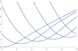
Figure 1. The eigenvalues $\lambda_{m}(b)$ plotted as functions of $b$. The graph indicates a non-diamagnetic effect: the function $b\mapsto\inf_{m\in\mathbb{Z}}\lambda_{m}(b)$ is not monotonic.

Acknowledgments The authors would like to thank M.P. Sundqvist for Fig. 1. This work started when AK visited the Laboratoire Jean Leray (Nantes) in January 2020 with the financial support of the programme Défimaths (supported by the region Pays de la Loire). The research of AK is partially supported by the Lebanese University within the project “Analytical and numerical aspects of the Ginzburg-Landau model”.

References

• [1] S. Fournais and M. Persson. Strong diamagnetism for the ball in three dimensions. Asymptot. Anal., 72(1-2):77–123, (2011).
• [2] B. Helffer. Semi-Classical Analysis for the Schrödinger Operator and Applications, volume 1336 of Nankai Institute of Mathematics, Tianjin, P.R. China. Springer-Verlag Berlin Heidelberg, 1998.
• [3] B. Helffer. The Montgomery model revisited. Colloq. Math., 118(2):391–400, 2010.
• [4] B. Helffer. Spectral theory and its applications, volume 139 of Cambridge Studies in Advanced Mathematics. Cambridge University Press, Cambridge, 2013.
• [5] B. Helffer and A. Kachmar. Eigenvalues for the Robin Laplacian in domains with variable curvature. Trans. Amer. Math. Soc., 369(5):3253–3287, 2017.
• [6] B. Helffer, A. Kachmar, and N. Raymond. Tunneling for the Robin Laplacian in smooth planar domains. Commun. Contemp. Math., 19(1):1650030, 38, 2017.
• [7] B. Helffer and Y. A. Kordyukov. Semiclassical spectral asymptotics for a two-dimensional magnetic Schrödinger operator: the case of discrete wells. In Spectral theory and geometric analysis, volume 535 of Contemp. Math., pages 55–78. Amer. Math. Soc., Providence, RI, 2011.
• [8] B. Helffer and Y. A. Kordyukov. Accurate semiclassical spectral asymptotics for a two-dimensional magnetic Schrödinger operator. Ann. Henri Poincaré, 16(7):1651–1688, 2015.
• [9] B. Helffer and A. Morame. Magnetic bottles for the Neumann problem: curvature effects in the case of dimension 3 (general case). Ann. Sci. École Norm. Sup. (4), 37(1):105–170, 2004.
• [10] A. Kachmar. On the ground state energy for a magnetic Schrödinger operator and the effect of the DeGennes boundary condition. J. Math. Phys., 47(7):072106, 32, 2006.
• [11] A. Kachmar. Diamagnetism versus Robin condition and concentration of ground states. Asymptot. Anal., 98(4):341–375, 2016.
• [12] A. Kachmar, P. Keraval, and N. Raymond. Weyl formulae for the Robin Laplacian in the semiclassical limit. Confluentes Math., 8(2):39–57, 2016.
• [13] A. Kachmar and M. P. Sundqvist. Counterexample to strong diamagnetism for the magnetic Robin Laplacian. arXiv:1910.12499, 2019.
• [14] D. Krejčiřík and N. Raymond. Magnetic effects in curved quantum waveguides. Ann. Henri Poincaré, 15(10):1993–2024, 2014.
• [15] K. Lu and X.-B. Pan. Surface nucleation of superconductivity in 3-dimensions. volume 168, pages 386–452. 2000. Special issue in celebration of Jack K. Hale’s 70th birthday, Part 2 (Atlanta, GA/Lisbon, 1998).
• [16] R. Montgomery. Hearing the zero locus of a magnetic field. Comm. Math. Phys., 168(3):651–675, 1995.
• [17] K. Pankrashkin and N. Popoff. Mean curvature bounds and eigenvalues of Robin Laplacians. Calc. Var. Partial Differential Equations, 54(2):1947–1961, 2015.
• [18] N. Raymond. Bound states of the magnetic Schrödinger operator, volume 27 of EMS Tracts in Mathematics. European Mathematical Society (EMS), Zürich, 2017.
• [19] N. Raymond and S. Vũ Ngọc. Geometry and spectrum in 2D magnetic wells. Ann. Inst. Fourier (Grenoble), 65(1):137–169, 2015.