GOBO: Quantizing Attention-Based NLP Models
for Low Latency and Energy Efficient Inference

Abstract.

Attention-based models have demonstrated remarkable success in various natural language understanding tasks. However, efficient execution remains a challenge for these models which are memory-bound due to their massive number of parameters. We present GOBO, a model quantization technique that compresses the vast majority (typically 99.9%) of the 32-bit floating-point parameters of state-of-the-art BERT models and their variants to 3 bits while maintaining their accuracy. Unlike other quantization methods, GOBO does not require fine-tuning nor retraining to compensate for the quantization error. We present two practical hardware applications of GOBO. In the first GOBO reduces memory storage and traffic and as a result inference latency and energy consumption. This GOBO memory compression mechanism is plug-in compatible with many architectures; we demonstrate it with the TPU, Eyeriss, and an architecture using Tensor Cores-like units. Second, we present a co-designed hardware architecture that also reduces computation. Uniquely, the GOBO architecture maintains most of the weights in 3b even during computation, a property that: (i) makes the processing elements area efficient, allowing us to pack more compute power per unit area, (ii) replaces most multiply-accumulations with additions, and (iii) reduces the off-chip traffic by amplifying on-chip memory capacity.

1. Introduction

Modern computing platforms, from servers to mobile and embedded devices, are energy constrained. Techniques for improving their energy efficiency can yield several benefits. They can reduce the energy footprint of data centers and as a result operating costs and environmental impact. They can increase uptime for mobile devices, and they can boost the capability of all systems by allowing them to perform more computations per unit of time. Improving energy efficiency is imperative for deep learning workloads as they are particularly compute and memory intensive. More so, given that the trend has been towards neural network models that require more computations and memory.

Memory accesses, be it off- or on-chip, account for a significant fraction of overall energy consumption when executing neural models. Memory footprint, bandwidth and energy limitations are most acute for attention-based models in language understanding tasks. Among them, the BERT family of natural language models (BERT, ) are today the benchmark delivering best-of-class accuracy. Their footprint, accesses, and execution time are dominated by the parameters (weights) of their numerous attention layers. The largest and most accurate among those models, BERT-Large has a footprint of 1.12GB, while BERT-base sacrifices some accuracy to reduce footprint to 326MB. These original BERT models are particularly expensive to train and use 32b floating-point parameters even for inference. Training BERT-Large on 16 Cloud TPUs (64 TPU chips) takes 4 days (BERT, ). For this reason, in typical applications we start with a pre-trained version which we then refine to a target task. Refinement time varies per task but usually takes hours to a few days for BERT-Large on an RTX 2080 Ti GPU. Several architecture modifications and quantization methods have been proposed to reduce the cost of BERT models (sanh2019distilbert, ; q-bert, ; intel8b, ). Generally, these methods require fine-tuning and often sacrifice accuracy. Quantization methods prolong training time by as much as $10\times$. It is for this reason that it is best to find model compaction methods that can work directly off the fine-tuned models.

We present a model compaction method, GOBO for such attention-based models. GOBO accepts as input a trained model and reduces the number of bits needed to represent its parameters be it weights or embeddings. GOBO maintains accuracy without any further model refinement such as retraining or fine-tuning. Fine-tuning requires access to the dataset which may not be available or may be not possible under strict time constraints (daily updates to the model).

GOBO compacts the original floating-point parameters representing the vast majority of them with 3b or 4b. GOBO is plug-in compatible with any execution engine for transformer models as after decoding it, GOBO produces a model with identical architecture (layer dimensions, types, and connectivity) containing floating-point parameters. GOBO can be used as an off- and potentially on-chip compression method to reduce footprint, traffic and energy and thus amplify bandwidth, capacity, performance and energy efficiency. GOBO can further boost performance and energy efficiency as it can simplify computation converting most multiplications in additions. Accordingly, as a second use of GOBO, we present a specialized functional unit that takes advantage of GOBO’s representation to reduce computation costs improving energy efficiency and performance.

We find that per layer the vast majority of weights closely follow some Gaussian distribution (whose parameters vary across layers), with very few — typically less 0.1% per layer — “outlier” weights being the exception. GOBO capitalizes on this phenomenon using a twofold approach: First, it stores the few outlier weights as-is. Second, GOBO uses a dictionary of very few — typically 8 — representative values (centroids) for all other weights. As a result, it stores the vast majority of the weights — typically 99.9% — as 3b indexes. GOBO uses a novel representative value selection algorithm that results in higher accuracy and is much faster to converge compared to linear partitioning or K-Means.

Deep Compression (han2015deep, ) is representative of a class of dictionary-based compression methods that have been used to compress the parameters of fixed-point models. It was originally demonstrated on 16b fixed-point convolutional neural networks. EIE takes advantage of Deep Compression to greatly boost energy efficiency when executing the resulting sparse neural networks (EIE, ). It stores weights as Huffman-encoded indexes into a dictionary of few representative values. The weights are expanded into their 16b fixed-point representative values before the MAC units. Compared to Deep Compression GOBO does not require fine-tuning, targets attention-based models which use floating-point values and where preserving outliers proves essential for maintaining accuracy, and uses a novel method for selecting the representative values. In addition, the GOBO hardware architecture never expands the quantized weights to their representative floating-point values.

Outlier-aware quantization targets fixed-point convolutional models (outlierAware, ; outlierAwareHW, ). Compared to GOBO, it requires determining in advance what fraction of values should be outliers, uses a much larger fraction of outliers, typically, 3%–5%, uses linear quantization to reduce datawidth for the non-outliers, and requires fine-tuning of the model. Fang et al., proposed a post-training quantization for convolutional neural networks (samsung20, ). They observed that the values tend to follow a bell-shaped distribution which they take advantage using a piece-wise linear quantization. GOBO targets attention-based models which are floating-point based, automatically adjusts the fraction of outliers using a Gaussian distribution fit, utilizes a novel fast converging method for selecting the non-uniform quantization values for the non-outliers, and requires no fine-tuning.

We evaluate GOBO on various datasets and state-of-the-art attention-based NLP models: BERT (two variants), DistilBERT (sanh2019distilbert, ), RoBERTa (two variants) (robetra, ), HAT (HAT, ), and SpanBERT (m2019spanbert, ). We also compare GOBO with two quantized BERT models, Q8BERT (intel8b, ) and Q-BERT (q-bert, ).

We highlight the following experimental findings:

• For the most challenging task in the GLUE (glue, ), MNLI, GOBO maintains accuracy while quantizing 99.9% of the weights to 3 bits.

• Our centroid selection algorithm converges $9\times$ faster than K-Means selection and consistently reduces the number of required centroids to half.

• A practical implementation of GOBO compression for off-chip memory reduces model footprint by $10\times$. For TPU this translates to $10\times$ performance.

• Under iso-compute-area constraints, the GOBO accelerator is on average $7\times$ faster and consumes $3\times$ less energy than an accelerator with TensorCore-like units.

2. The BERT Family of NLP Models

Google’s BERT (BERT, ) (Bidirectional Encoder Representations from Transformers) is an attention-based model that is the model of choice for a variety of NLP tasks.

BERT-Large and BERT-Base: Training deep learning models capable of state-of-the-art accuracy on NLP tasks is expensive in terms of time, energy and volume of data. nvidia reports that to train BERT from scratch in less than 1 hour, a cluster with 1,472, V100 GPUs was required (narasimhan_2019, ). Each V100 GPU has 32GB of memory and consumes 450W at a total power cost of $662KW$ for the GPUs alone. To enable practical deployment for several tasks without access to such computing power and budgets the BERT framework introduced a “pre-training and fine-tuning” approach. BERT is pre-trained once on an unlabeled dataset —billions of words— and then the pre-trained model can be fine-tuned for a few epochs to perform various tasks. Two pre-trained BERT models have been released: BERT-Base and BERT-Large. BERT-Large typically achieves higher accuracy leveraging $3.5\times$ more parameters.

Tasks: BERT is most useful in language understanding tasks, such as sentiment analysis, paraphrasing, sentence similarity detection, and question answering. GLUE (glue, ) (General Language Understanding Evaluation) and SQuAD (squad, ) (Stanford Question Answering Dataset) are two popular benchmarks for such tasks. In this study, we focus mostly on the MNLI (The Multi-Genre Natural Language Inference) task of GLUE, since a) it is the most comprehensive inference task in the dataset, and b) it is the most sensitive task to quantization (BERTsurv, ). MNLI given two provided sentences, the premise and the hypothesis, predicts if the premise entails the hypothesis, contradicts with it, or neither. As a representative of other less sensitive to quantization tasks in GLUE, we evaluate STS-B (Semantic Textual Similarity Benchmark) which tries to predict the similarity score between two human-annotated sentences. We use MNLI for all models since we are able to fine-tune BERT on the hardware that is available to us. Unfortunately, this is not possible for SQuAD. Its dataset is among the largest ones that are available and fine-tuning BERT for it is not practical on a single GPU. However, we had access to fine-tuned BERT-Large and SpanBERT models on SQuAD, and since our method does not require fine-tuning, we do evaluate GOBO on SQuAD for these models. We further evaluate GOBO on an English to French translation task using a Transformer model (HAT).

BERT Architecture: BERT-base consists of 12 BERT Layers while BERT-large has 24. Figure 1a shows that each BERT layer has 3 components: Attention, Intermediate, and Output. Each component includes a series of fully connected layers (FC) followed by a single normalization layer. The hidden state is a 768- to 1K-element vector (size varies per model and layer). After the last BERT layer, there is a single FC layer, the Pooler. Table 2 details the configuration of these models. In total, BERT-Base has 73 ($\mathit{12\times 6+1}$) FC layers and 110M parameters, whereas BERT-Large has 145 ($\mathit{24\times 6+1}$) and 340M parameters. Activations and weights are 32b floating-point numbers and Table 2 reports the resulting memory footprint. Since BERT consists of mostly FC layers, and since the hidden state is a relatively short vector, it is the weights that dominate memory footprint and have to be streamed from off-chip. A set of embedding tables map the raw input into the vectors the network uses.

Table 1. BERT Architecture

	BERT-Base		BERT-Large
BERT layers	12		24
Component	FC #	Dimensions	FC #	Dimensions
Attention	4x	768 x 768	4x	1024 x 1024
Intermediate	1x	768 x 3072	1x	1024 x 4096
Output	1x	3072 x 768	1x	4096 x 1024
BERT Pooler	768 x 768		1024 x 1024

Table 2. BERT Memory Footprint

Model	BERT-Base	BERT-Large
Embedding Tables	89.42 MB	119.22 MB
Weights	326.26 MB	1.12 GB
Model Input per Word	3 KB	4 KB
Largest Layer Acts per Word	12 KB	16 KB
Sequence Length	128	128
Activations	1.5 MB	2 MB

(a) BERT layer architecture. Boxes are FC layers.

(b) Per layer weight distribution

(c) Weights of a BERT layer

Figure 1. BERT layer architecture and per layer weight values.

BERT Derivatives: BERT variants have been since released improving accuracy or reducing size. DistilBERT (sanh2019distilbert, ) uses knowledge distillation over the pre-trained BERT models to train a smaller, yet similar architecture. Facebook’s RoBERTa (robetra, ) uses hyperparameter tuning, a different training method and a different embedding table to improve accuracy while maintaining the same architecture. We also compare GOBO to two state-of-the-art quantized BERT variants, Intel’s Q8BERT (intel8b, ) which uses 8b fixed-point values, and Q-BERT (q-bert, ) which uses dictionary compression.

Per Layer Weight Distribution: Figure 1b shows the distribution of the weights for a few layers of BERT-Base which are representative of the shape of the distributions for the other layers. In every layer the weights closely follow a Gaussian distribution which can be described by the mean and standard deviation of the layer’s weights. The Gaussian-like distribution of parameters was observed in various DNNs (samsung20, ; G_DNN, ; G_DNN2, ; gordon2020compressing, ). Figure 1c shows a color coded representation of a layer’s weights (one per x coordinate) based on the probability of each weight belonging to the layer’s Gaussian distribution. This reveals that there is a tiny fraction of weights that are on the fringes of the Gaussian distribution as their magnitude is considerably larger than the rest of the weights.

These observations motivate GOBO which splits the weights of each layer into two groups. The “G” (Gaussian) group consists of weights whose magnitude fits within 99.9% of the values as described by the Gaussian distribution formed by the mean and standard deviation of all weights in the layer. The second group, the “Outliers” (“O”) includes values that fall outside the Gaussian distribution. We have found experimentally that: (1) representing just the outliers precisely and quantizing the rest of the model to a few representative values (e.g, 8) is sufficient for maintaining model accuracy. (2) Using representative values for all weights either drastically reduced compression (too many representative values were needed) or sacrificed accuracy.

3. Related Work

Compression methods for NLP models fall under three different approaches, Model Quantization, Pruning, and Knowledge Distillation. In model quantization the objective is to reduce the number of bits for representing the model’s parameters while keeping the model architecture as-is. Pruning’s goal is to remove some of the weights by forcing them to be zero. Combining pruning with zero-aware memory encoding often reduces the model’s footprint. Knowledge distillation trains a smaller model, the student, to mimic the behaviour of a much larger teacher model.

Model Quantization: Quantization techniques can be direct or indirect. Direct methods map the weights to a fixed-point representation, whereas indirect methods use a dictionary of representative values and encoded weights as indexes.

Intel’s Q8BERT introduces a fine-tuning method to quantize the weights and activations to 8-bit fixed-point values (intel8b, ). Some operations such as Softmax and Layer Normalization are not quantized and use FP32. We compare the accuracy of GOBO with Q8BERT on the MNLI task in Section 4.3 showing that GOBO reduces model size more than Q8BERT while maintaining accuracy. Furthermore, GOBO is faster to deploy since it does not require fine-tuning. Although, the decompressed model with GOBO uses FP32 values, the GOBO hardware accelerator performs most computations without decompressing the weights.

Q-BERT is a dictionary based fine-tuning approach that uses second order Hessian information to quantize the model’s weights to a few (4 to 16) representative values. It stores weights as indexes to those values (q-bert, ). Q-BERT separates the weights of each layer into multiple groups and quantizes each group separately using per group dictionaries each of 4, 8 or 16 entries. Dividing each layer in 128 groups results in acceptable accuracy. Finally, Q-BERT quantizes the embedding tables to 8b to avoid a significant loss in accuracy. GOBO does not require fine-tuning, only keeps one dictionary per layer and quantizes the embedding layers to 3b. Section 4.3 shows that GOBO achieves higher compression than Q-BERT while maintaining accuracy.

Model Pruning: Weight pruning reduces model footprint by forcing a portion of the weights to be zero. Gordon et al., studied pruning BERT during training (gordon2020compressing, ). They showed that 30%-40% of the weights based on the magnitude could be pruned with minimal effect on the accuracy of the final task. They found that MNLI was the task that was most sensitive to pruning. Structured pruning removes a series of weights that correspond to a component of the model (BERTsurv, ). Attention head pruning (darksecret, ; raganato2020fixed, ) and Encoder unit pruning (fan2019reducing, ) are examples of this approach. Pruning methods require fine-tuning to compensate for the initial accuracy loss. As we will show, GOBO achieves nearly $10\times$ compression (99.9% of 32b values are compressed to 3b). Even if we ignore its encoding overhead, a pruning method should remove nearly 90% of the weights to achieve similar compression. GOBO could complement pruning an investigation left for future work.

Knowledge Distillation: Knowledge distillation trains a smaller model (student) from a larger model (teacher). Based on what the student learns from the teacher there are three groups of Knowledge distillation approaches for BERT (BERTsurv, ) currently in use. In the first group, the student learns the behaviour of the encoder layer. The student can have fewer attention heads in each layer (zhao2019extreme, ; sunmobilebert, ; jiao2019tinybert, ) or fewer encoder layers (sanh2019distilbert, ; sun2019patient, ). Another approach trains a student based on the output logits (input of the last layer’s softmax) (cheng2017survey, ). Furthermore, The student is free to adopt a different type of network or components thereof such as a Convolutional Neural Network (CNN) or Long Short Term Memory (LSTM). Tang et al., used a Bidirectional LSTM (BiLSTM) based architecture to replace the attention layers (tang2019distilling, ; tang2019natural, ). Chia et al., proposed a CNN-based model to replace transformer layers where the student tries to learn the contextual dependence of the tokens (words) from the output of each attention layer (chia2019transformer, ). DistilBERT (sanh2019distilbert, ) is distilled model of BERT-Base and is about half in size. Section 6 shows that GOBO compresses DistilBERT by $10\times$ and results in a model that is $20\times$ smaller than BERT-Base.

4. GOBO Quantization

For BERT, GOBO operates at the granularity of a layer and over the fine-tuned model. The compaction process starts with separating the weights into two groups, the “Gausian” (G) and the “Outliers” (O). GOBO stores the outliers as-is (FP32) whereas it quantizes the “G” group values to a few representative values. Only a tiny fraction of the weights, typically less than 0.1%, end up in the “O” group. GOBO reduces overall model size by quantizing the Gaussian group. Since the weight distribution is not uniform, we propose a non-linear quantization method that results in higher resolution where the weights are densely populated. This method proves capable of encoding roughly 99.9% of the weights with just 8 representative FP32 values, while the inference error is kept below 1% (or with 16 representative values for no accuracy loss). A “G” group weight is stored as a 3b index to those representative values. GOBO uses just one set of representative values per layer.

In summary, GOBO stores the following information per layer: (1) The outliers in original form. (FP32) (2) The bin index for each “G” group weight. (3b) (3) A reconstruction table for weights which represents the representative values (centroids) for each bin. (FP32) We defer the description of a practical encoding until Section 5 and after we discuss the “G” and “O” group selection and quantization process.

4.1. Outlier Detection

To detect the outlier weights for an FC layer, GOBO first computes the mean and the standard deviation of the layer’s weights. Then per weight, it computes a probability that the weight belongs to that distribution using the PDF (Eq. 1) where $x$ is the weight, $\mu$ is the mean, and $\sigma$ is the standard deviation. GOBO uses a threshold, a configuration parameter, to select outliers. A weight whose probability is less than the threshold is deemed as an outlier. We empirically found that a log-probability threshold of -4 is sufficient for maintaining overall accuracy.

(1) $$\footnotesize\mathit{pdf}(x|\mu,\sigma^{2})=\frac{1}{\sqrt{2\pi\sigma^{2}}}e^{-\frac{(x-\mu)^{2}}{2\sigma^{2}}}$$

The closest prior work to GOBO’s outlier selection approach is outlier-aware quantization (outlierAware, ; outlierAwareHW, ). This method targets fixed-point CNNs and considers a fixed, predetermined fraction of the weights (at least 3% which is an order of magnitude more than GOBO) as outliers. The outliers remain in 16b and non-outlier values are linearly quantized to 4b. To reduce the quantization error, fine-tuning is required. With GOBO’s nonlinear quantization having about 1 outlier every 1000 weights proves sufficient for preserving accuracy without fine-tuning. In addition, GOBO uses dictionary-based compression of the non-outlier group. Section 4.3 compares GOBO with an outlier-aware inspired method that uses Linear Quantization for the non-outliers.

4.2. “G” Group Weight Quantization

GOBO’s aims to represent the “G” weights with few representative FP32 values. This amounts to clustering the weights and assigning a representative value per cluster. We use clusters of equal population. Intuitively, this objective will put more clusters where weights are densely populated affording higher resolution where there are more weights. This approach can be implemented by sorting the weights and dividing them to equally sized clusters. The first and the last weight in each cluster determine the boundaries of that cluster. Then the average of the weights inside each cluster can be used as the centroid. We find that quantizing BERT-Base with this approach into 8 clusters (3b indexes) degrades inference accuracy by 10% in GLUE tasks.

To reduce this error GOBO uses an iterative approach that bears similarity to K-Means. The process repeatedly applies the following two steps: 1) GOBO moves a weight from cluster A to cluster B if the $L1$ distance of the weight and the centroid of cluster A is greater than the $L1$ distance of the weight and the centroid of cluster B. 2) After re-assigning the weights to clusters, GOBO updates the centroids by computing the new average over the weights of each cluster. This is equivalent to minimizing the $L2$ distance. This iterative process repeats until the sum of $L1$ distances between centroids and weights is minimized. For a 3b quantization, we observed that 7 iterations are enough to converge to the optimal solution.

Terminating the process using the $L1$ proves faster and results in a model with higher inference accuracy using the $L2$. Figure 4 helps explaining why this is so. The figure shows how the $L1$ and $L2$ evolve over time (iterations) and also the cumulative distribution of weight-to-bin reassignments. Weight reassignments follow Zipf’s law with more than 80% of them happening in the first 15% of iterations. This explains the initial rapid drop in $L1$ which the first step of each iteration directly minimizes. Since reducing the $L1$ also reduces $L2$ (but not vice versa) this also improves $L2$. The second step reassigns centroids to minimize $L2$ instead. As the figure shows, this reassignment proceeds much more slowly and quickly hurts $L1$ as it overemphasizes weights that are further away from the centroid. Given the Gaussian distribution, these weights disproportionately affect centroid selection reducing representation accuracy for all weights. Terminating when $L1$ is minimized better balances the per value representation accuracy. Empirically, emphasizing all weights equally rather the overemphasizing a few, results in better overall inference accuracy. GOBO’s approach converges $9\times$ faster than K-Means and as Section 4.3 describes achieves higher accuracy.

Deep Compression uses dictionary compression for CNNs utilizing K-Means with linear initialization for cluster centroids and requiring fine-tuning to regain any accuracy loss (han2015deep, ). It minimizes the $L2-Norm$ inside each cluster. GOBO maintains the model’s accuracy without any help from retraining. The centroid initialization in GOBO is nonlinear and depends on the per layer weight distribution. GOBO detects a few but effective outliers and keeps them in their original representation. importantly, GOBO objective is to minimize $\mathit{L1\mathchar 45\relax Norm}$ within each cluster rather than $L2$. Algorithm 1 summarizes how GOBO compacts each layer.

Figure 2. GOBO and K-Means convergence.

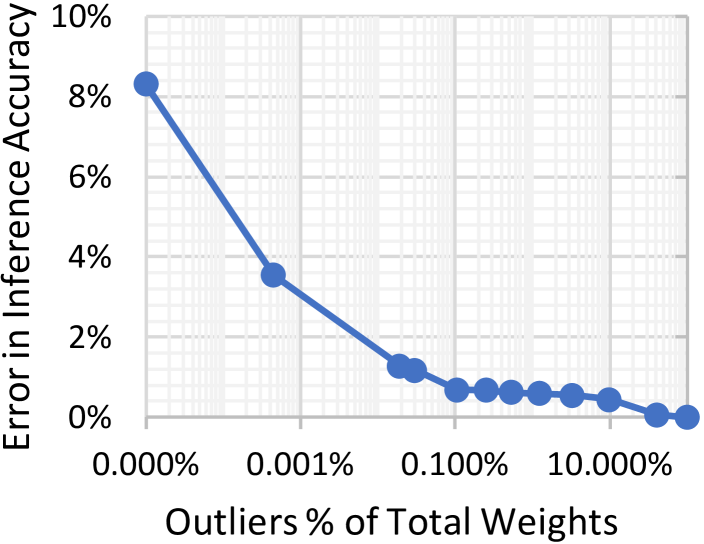
Figure 3. Outlier’s impact on inference accuracy of BERT-Base (MNLI)

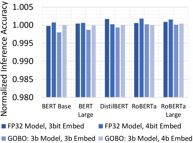
Figure 4. Effect of Embedding Table Quantization on Accuracy.

1Compute the mean$(m)$ and standard deviation$(sd)$ of the weights;

2 Detect outliers based on the Gaussian dist. specified by $m$ and $sd$;

3 Store outlier weights as-is;

4 Sort the “G” weights and place them into bins with equal capacity;

5 Compute the min, max, and mean (centroid) of each bin;

6 $L1_{new}\leftarrow$ L1-Norm of the current assignment;

7 do

8       $L1_{old}\leftarrow L1_{new}$;

9       Reassign weights the closest centroid;

10       Update centroids based on the new assignment;

11       $L1_{new}\leftarrow$ L1-Norm of the current assignment;

12      

13while $L1_{old}\geq L1_{new}$;

Algorithm 1 GOBO Quantization

4.3. Accuracy and Compression Potential

This section evaluates GOBO’s effect on accuracy and compression rate. Here we ignore the additional information that any practical encoding will require. We introduce a specific encoding in Section 5 where we use GOBO for off-chip memory compression. As it will be shown, the overhead is tiny which is no surprise as it includes the representative values and the coordinates of the outliers.

Methodology: We use the pre-trained models, the scripts and datasets provided by the Hugging Face repository (Wolf2019HuggingFacesTS, ) and the SciKit-Learn library. Specifically, to fit a Gaussian distribution we use sklearn.GaussianMixture with one Gaussian component. Then the log probability for each weight is computed using score-samples. We considered the weights with the log probabilities of $\mathchar 45\relax 4$ or less as outliers.

To show the advantage of GOBO’s clustering approach we compare the accuracy of each model when the “G” weights are quantized by Linear Quantization and K-Means. In linear quantization, the range of non-outlier weights (“G” group) is linearly divided by the number or bins ($2^{Bits}$). In K-Means we use the same centroid initialization as GOBO and iterate until the cluster assignments converge. The outlier weights in all of these methods are detected and represented in the same manner. All experiments we performed on a dual RTX 2080 Ti 11GB GPU system with an AMD Ryzen Threadripper 1920X CPU with 128GB Quad-channel DDR4-3200 RAM.

Importance of Outliers: Figure 4 reports the absolute loss in inference accuracy of 3-bit quantized BERT-Base on MNLI when the fraction of outliers is swept from 0% to 100%. GOBO without outliers incurs an 8.3% accuracy loss. Having just 0.1% of outliers reduces this loss to less than 1%. Increasing the number of outliers by $100\times$ to 10% improves accuracy by just 0.25%.

BERT-Base: First we compare GOBO to other BERT-specific quantization methods. In this section we focus on the MNLI task which is the most challenging among the GLUE set of tasks. Table 6 shows accuracy on the MNLI task with different quantization methods: Intel’s Q8BERT (intel8b, ), Q-BERT (q-bert, ), and GOBO with 3b or 4b “G” weights. Recall that Q-BERT and Q8BERT require fine-tuning. Using the Hugging Face PyTorch library, fine-tuning BERT-Base for the MNLI task on our dual GPU system took about 3 hours per epoch. We fine-tuned the model for 3 epochs as suggested by the Hugging Face documentation. After 3 epochs (9 hours) we achieved the baseline accuracy of 84.45%. Fine-tuning the same task on the same machine for Q8BERT, takes about 34 hours per epoch. Based on the authors’ suggestion, we trained the model for 3 epochs (102 hours). Quantizing the same model with GOBO takes about 10 minutes using a single CPU core of our system.

The results show that GOBO can compact the model by $9.8\times$ and with less than 0.7% loss in accuracy and by $7.92\times$ with no accuracy loss. Q-BERT compacts the model by $6.5\times$ at a $0.56\%$ accuracy loss or by $7.81\times$ with a $1.04\%$ accuracy loss. Q8BERT reduces the model the least and by $4\times$ at a $0.7\%$ accuracy loss. Recall, however, that it uses 8b fixed-point. In summary, GOBO produces models that are smaller and with similar or no accuracy loss, and produces the model within minutes vs. days.

We next show that our proposed centroid selection method for the “G” group is better than two prior methods: linear quantization and K-Means. We study GOBO with our proposed quantization, GOBO with linear quantization, and GOBO with K-Means quantization. We study how accuracy is affected as we change the number of centroids (all experiments have the same set of outliers). Tables 6 shows that GOBO as proposed when using 3b weights (8 centroids) incurs an accuracy loss of 0.69% which is considerably less than then 1.36% loss incurred with K-Means. Linear quantization performs the worst incurring an error of nearly 52%. To maintain the baseline accuracy, GOBO, K-Means and Linear Quantization require, 4b, 5b, and 6b weight indexes respectively. We note that using 4b weight indexes amounts to a 33% increase over using 3b. Moreover, our proposed selection method is faster than K-Means.

Similar behavior is observed for the STS-B task as Table 6 shows. As expected STS-B is less sensitive to quantization. GOBO incurs no accuracy loss with 3b, whereas K-Means needs 4b and linear quantization requires 5b.

Table 3. Comparison of GOBO and BERT-Specific Quantization Methods. BERT-Base on MNLI.

BERT-Base (MNLI)	Weights	Embedding	Accuracy (m)	Error	No Fine-tuning	Compression Ratio
Baseline	FP32	FP32	84.45%	-	-	1$\times$
Q8BERT (intel8b, )	8-bit	8-bit	83.75%	0.70%	✗	4$\times$
Q-BERT (q-bert, )	3-bit	8-bit	83.41%	1.04%	✗	7.81$\times$
Q-BERT (q-bert, )	4-bit	8-bit	83.89%	0.56%	✗	6.52$\times$
GOBO	3-bit	4-bit	83.76%	0.69%	✓	$\textbf{9.83}\mathbf{\times}$
GOBO	4-bit	4-bit	84.45%	0.00%	✓	$\textbf{7.92}\mathbf{\times}$

Table 4. GOBO w/ “G” Group Centroid Selection Policies: BERT-Base/-Large.

	Baseline	GOBO w/ Linear Quant.		GOBO w/ K-Means		GOBO		Potential Comp. Ratio
GLUE/MNLI with BERT-Base
Bits		Accuracy (m)	Error	Accuracy (m)	Error	Accuracy (m)	Error	Potential Comp. Ratio
32	84.45%	-	-	-	-	-	-	1$\times$
2	-	31.81%	52.64%	69.98%	14.47%	71.02%	13.43%	16$\times$
3	-	32.48%	51.97%	83.09%	1.36%	83.76%	0.69%	10.67$\times$
4	-	82.75%	1.70%	84.01%	0.44%	84.45%	0.00%	8$\times$
5	-	84.20%	0.25%	84.45%	0.00%			6.4$\times$
6	-	84.45%	0.00%					5.3$\times$
GLUE/STS-B on BERT-Base
Bits		Spearman	Error	Spearman	Error	Spearman	Error	Potential Comp. Ratio
32	88.33%	-	-	-	-	-	-	1$\times$
2	-	2.67%	85.66%	81.12%	7.21%	82.66%	5.67%	16$\times$
3	-	74.00%	14.33%	88.11%	0.22%	88.33%	0.00%	10.67$\times$
4	-	87.46%	0.87%	88.33%	0.00%			8$\times$
5	-	88.33%	0.00%					6.4$\times$
SQuAD v1.1 with BERT-Large
Bits		F1 Score	Error	F1 Score	Error	F1 Score	Error	Potential Comp. Ratio
32	91.95%	-	-	-	-	-	-	1$\times$
2	-	0.01%	91.94%	34.83%	57.12%	56.22%	35.73%	16$\times$
3	-	5.37%	86.58%	90.56%	1.39%	91.04%	0.91%	10.67$\times$
4	-	89.11%	2.84%	91.24%	0.71%	91.95%	0.00%	8$\times$
5	-	90.61%	1.34%	91.92%	0.03%			6.4$\times$
6	-	91.88%	0.07%	91.95%	0.00%			5.3$\times$
7	-	91.95%	0.00%					4.57$\times$

Table 5. GOBO w/ “G” Group Centroid Selection Policies: GLUE/MNLI on DistilBERT.

Bits	Baseline	GOBO w/ K-Means		GOBO		Potential
	Accuracy (m)	Accuracy (m)	Error	Accuracy (m)	Error	Comp. Ratio
32	81.98%	-	-	-	-	1$\times$
3	-	80.83%	1.15%	81.30%	0.68%	10.67$\times$
4	-	81.78%	0.20%	81.98%	0.00%	8$\times$
5	-	81.98%	0.00%			6.4$\times$

Table 6. GOBO w/ “G” Group Centroid Selection Policies: GLUE/MNLI on RoBERTa.

RoBERTa-Base							RoBERTa-Large
Bits	Baseline	GOBO w/ K-Means		GOBO		Potential	Baseline	GOBO w/ K-Means		GOBO		Potential
	Acc. (m)	Acc. (m)	Error	Acc. (m)	Error	CR	Acc. (m)	Acc. (m)	Error	Acc. (m)	Error	CR
32	87.60%	-	-	-	-	1$\times$	90.20%	-	-	-	-	$1\times$
3	-	76.00%	11.60%	79.68%	7.92%	10.67$\times$	-	82.18%	8.02%	84.26%	5.94%	10.67$\times$
3b/4b				86.19%	1.41%	10.13$\times$	-			89.33%	0.87%	10.03$\times$
4	-	86.80%	0.80%	87.30%	0.30%	8$\times$	-	89.48%	0.72%	89.88%	0.32%	8$\times$
5	-	87.32%	0.28%	87.60%	0.00%	6.4$\times$	-	90.07%	0.13%	90.20%	0.00%	6.4$\times$
6	-	87.60%	0.00%			5.3$\times$	-	90.20%	0.00%			5.3$\times$

BERT-Large: To our knowledge, ours is the first attempt to quantize BERT-Large on the SQuAD task. SQuAD is a complex task that requires days of fine-tuning when implemented over BERT-Large. We apply GOBO after this fine-tuning phase at a negligible cost in time. Table 6 reports the compression and accuracy of the model with different “G” group quantization policies. Our centroid selection policy proves best. With 3b weight indexes the accuracy loss is less than 1% and with 4b there is none. For MNLI, GOBO incurs no accuracy loss even with 3b weight indexes. In the rest of this section we limit attention only to GOBO w/ K-means and GOBO with our proposed centroid selection policy.

DistilBERT: Table 6 shows accuracy when quantizing DistilBERT which was distilled from BERT-Base and is about $2\times$ smaller. GOBO incurs no or less than 1% accuracy loss with 4b and 3b weights respectively resulting in models that are $16\times$ or $21\times$ smaller than BERT-Base. In either case, K-Means requires twice as many bins.

RoBERTa: Table 6 shows accuracy and compression ratio. Quantizing to 3b “G” weights incurs an accuracy loss of 8%. Two FC layers (”Value layer” in self-attention and Intermediate layer) in the first 6 BERT Encoders are the most sensitive to quantization. We can either quantize the whole model to 4b “G” weights (accuracy loss of just 0.6%), or better, we can use 4b “G” weights just for these two layers for the first 6 out of the 12 total Encoder layers and 3b for the rest. This reduces the accuracy loss to just 1.4%.

RoBERTa-Large: achieves a score of 90% on MNLI and, as Table 6 shows, is less sensitive to quantization compared to the RoBERTa. By quantizing the Value and Intermediate layers to 4b for the first 14 Encoders (out of 24) and to 3b for the rest GOBO achieves less than 1% loss in accuracy.

Table 7. HAT model size (M), embedding (E) and compression ratio (CR).

HAT: WMT’14 En-Fr	BLEU	Error	M(MB)	E(MB)	M CR	CR
Baseline FP32 (HAT, )	41.8	-	227	217	1.0$\times$	1.0$\times$
KMeans 4-bit (M) (HAT, )	41.1	0.7	28	217	8.0$\times$	1.8$\times$
GOBO 4 bit (M)	41.5	0.3	29	217	7.8$\times$	1.8$\times$
GOBO 4-bit (E+M)	41.4	0.4	29	28	7.8$\times$	7.8$\mathbf{\times}$

Table 8. SpanBERT FP16 model quantization.

SpanBERT	SQuAD v1.1		SQuAD v2		CR
	F1 Score	Error	F1 Score	Error
Baseline FP16	93.96%	-	88.68%	-	1.00$\times$
GOBO 3-bit	93.15%	0.81%	88.68%	0%	5.31$\times$
GOBO 4-bit	93.94%	0.02%	88.76%	-0.08%	3.99$\times$

Table 9. Embedding size (MB) and compression ratio (CR).

	Baseline	GOBO
Model/Task	FP32	3-bit	CR	4-bit	CR
BERT-Base/MNLI	89.42 MB	8.63	10.36$\times$	11.42	7.83$\times$
BERT-Large/SQuAD v1.1	119.22 MB	11.26	10.59$\times$	14.98	7.96$\times$
DistilBERT/MNLI	89.42 MB	8.85	10.10$\times$	11.63	7.69$\times$
RoBERTa/MNLI	147.26 MB	14.18	10.38$\times$	18.77	7.84$\times$
RoBERTa-Large/MNLI	196.34 MB	18.41	10.66$\times$	24.55	8.00$\times$

HAT: We evaluated GOBO on HAT produced models (HAT, ). HAT is a neural architecture search (NAS) method that composes Transformer models for efficient language translation on various hardware platforms. HAT designs FP32 models; however, the authors report accuracy when the model is quantized using KMeans with linear initialization and for a maximum of 300 iterations (similar to Deep-compression (han2015deep, )). Table 9 shows the BLEU score on the WMT’14 En-Fr, English to French translation task when it is quantized by KMeans (as reported by the authors (HAT, )) and GOBO. GOBO quantization achieves 0.4 higher BLEU score at the expense of less than 1% extra footprint for the outliers. If embedding tables are also quantized with GOBO the compression ratio rises to $7.8\times$. GOBO proves effective for an attention model (different than the BERT family) where it outperforms a state-of-the-art dictionary-based quantization method.

SpanBERT: Certain architectures introduced 16b floating-point arithmetic (FP16 or Bfloat16) targeting deep learning training and inference. In general, BERT models are trained with FP32. However, Facebook’s SpanBERT is a BERT-derived model that has been successfully trained to work with FP16. Table 9 evaluates GOBO SpanBERT (m2019spanbert, ) on the SQuADv1.1 and SQuADv2 datasets. GOBO with 3b matches the baseline accuracy on SQuADv2 and incurs less than 1% error in SQuADv1.1. GOBO achieves a $5.31\times$ compression ratio. This result shows that GOBO remains effective even when using FP16 is possible.

Embedding Table Quantization: GOBO can also be used to quantize the embedding tables. Table 9 shows the size of embedding table before and after quantization. The outlier threshold for all of these experiments is set to $\mathchar 45\relax 4$. Figure 4 compares the inference accuracy of each model in two scenarios: in the first, we quantize the embedding layer only and keep the model weights in their original FP32 representation. This experiment illustrates the effect of embedding quantization on the original model’s accuracy. This approach not only maintains the model’s accuracy but, in certain cases, improves it. In the second scenario, we apply GOBO quantization throughout. While the FC layers’ weights are quantized to 3b, using 4b embedding maintains accuracy, whereas 3b incurs a 0.2% accuracy loss.

5. Memory Compression

This section presents the first practical application of GOBO where it is used to compress weights in off-chip memory. As a result GOBO reduces memory traffic and energy and increases effective memory capacity. Regardless, of the dataflow used, the weights of each layer will be accessed sequentially, in large enough chunks to maximize reuse. Accordingly, a format that supports streaming accesses into the weight matrix is sufficient. There is no need to support random accesses. We use the example weight matrix of $768\times 768$ of Figure 5a to explain how GOBO encodes values in memory and how it decompresses them. For an arbitrary dataflow, assume the weight matrix is divided into $16\times 16$ submatrices (SM) of 256 weights each. Each SM is divided into 16 blocks where each block contains the weights that are going to be processed together by some data-parallel functional unit, e.g., a GPU shared multiprocessor, and thus need to be stored together in on-chip memory.

With GOBO, the main challenge is handling outliers. Fortunately, we can still maintain long sequential accesses off-chip thus not sacrificing bandwidth utilization. Figure 5c shows the GOBO container comprising three sections: Header, Quantized Weights, and Outliers. The header contains the metadata describing the dimensions of the layer, the number of bits used per weight index, followed by the centroid table. The figure shows only the centroid table and assumes 8 centroids. Padding is used to keep the Quantized Weights section that follows properly aligned to a memory row. This section contains the weight indexes which are stored in exactly the same order as the original FP32 weights would have been. However, GOBO stores just a 3b per weight including the outliers. However, for the outliers the index is ignored and is superseded by the Outliers section. For instance, the third weight in $SM_{0}-B_{0}$ is an outlier, and a dummy $"000"$ index is stored for it. This format maintains the relative position of weights and avoids the hardware support and run-time costs of data movement and re-alignment during decompression.

The Outliers section encodes the outliers in submatrix order. Each SM begins with an outlier count (8b supporting up to 256 outliers) followed by the outliers in block order. Each outlier is encoded with a triplet $(B,W,V)$ where $B$ (4b) is the relative block within the SM, $W$ is the weight offset (4b) within the block, and $V$ is the FP32 value. In our example, $SM_{0}$ contains $2$ outliers with the first replacing the third weight in block 0 (dashed arrow).

To make quantization transparent to the processing elements, the decompression engine generates a stream of FP32 weights. The decompression engine requires two concurrent sequential access streams. The first reads the Header and then the Quantized weights. The Header is used to set the lookup tables (LUT) in the decompression engine. There is one LUT per weight that we want to decompress concurrently, a configuration parameter. Once the header is read, the first stream processes the weight indexes placing them in a FIFO which feeds the LUTs that replace them with the appropriate centroids. Concurrently, the second stream reads in the Outliers section placing values in another FIFO. Using the information per outlier, the outliers selectively overwrite the LUT provided values. Since outliers are rare, processing at most one per cycle proves sufficient.

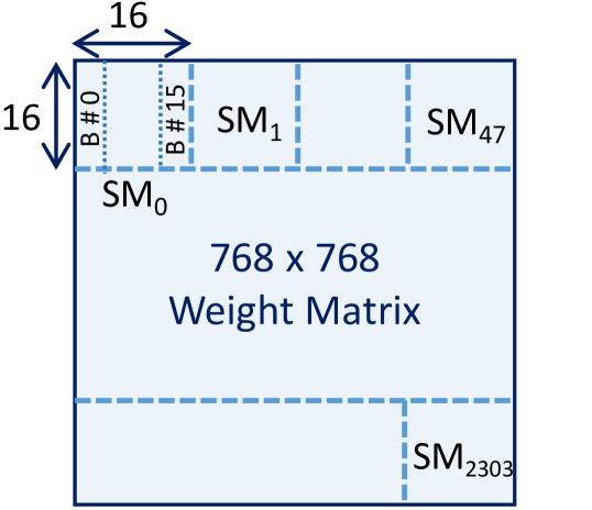
(a) Weight Matrix

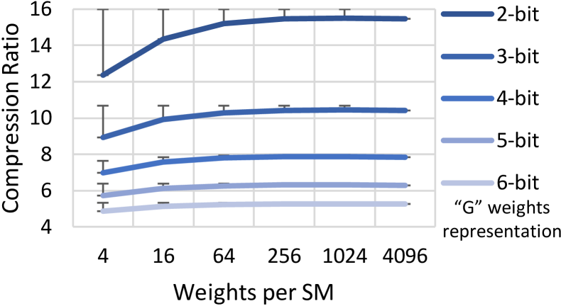
(b) Effect of SM size on Compression Ratio

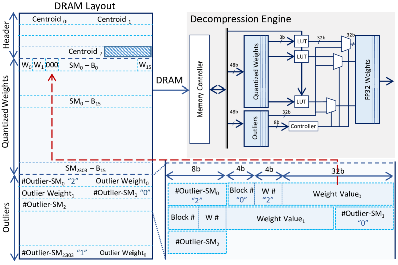
(c) DRAM Layout and Decompression Engine

Figure 5. GOBO Memory Compression.

Figure 5b justifies our choice of $16\times 16$ submatrices. It shows the compression ratio for the BERT-Base model for various SM sizes and for weight quantizations of 2b to 6b. The error bars show what the compression rate would have been if there were no outliers at all. In this case, every weight would be represented by $log_{2}(\#bins)$ bits. This representation serves as a useful measure for judging how well the method works. The measurements show that using SMs of 256 weights or more, achieves nearly the maximum possible compression ratio for all weight quantization widths.

The described memory layout is suitable when the dataflow is pre-determined making sequential accesses to all components possible. To allow the dataflow to change without changing the layout, minor changes to the Outlier memory layout are sufficient. The outlier counts and the outliers can be stored separately into two linear arrays $C$ and $O$ respectively. $C$ contains the counts in cumulative form (entry $C_{i}$ reports the number of outliers before the ith SM) so that they can serve as indexes into $O$. To access the outliers of the ith SM, an extra memory reference will first read $C_{i}$ and use it as an index to start fetching the outliers from $O$. The number of outliers contained in the SM is given by $C_{i+1}-C_{i}$.

6. Compute Acceleration

Most of the computation occurs in the FC layers, each of which is a weight matrix and activation vector multiplication. The use of a very small dictionary allows us to transform the computation from many “lookup to translate weight index to its FP32 centroid followed by a multiply-accumulate with an FP32 activation” (one per weight) to an FP32 activation accumulation per weight index followed by a few FP32 multiply-accumulate operations (one per centroid per output activation). That is, rather than first decoding each weight to its centroid and then multiplying with the corresponding activation, we can instead, given a weight index, accumulate the corresponding activation into a per centroid sum, and after doing so for all quantized weights, we can multiply just these few sums with the centroids. Consider for example, a layer with 4 input activations $A_{i}$ and one output activation $OA$. When weights are not quantized this rudimentary FC layer performs the computation in Eq. 2.

(2) $$\scriptsize OA ={{A}_{1}}{{W}_{1}}+{{A}_{2}}{{W}_{2}}+{{A}_{3}}{{W}_{3}}+{{A}_{4}}{{W}_{4}}$$

(3) $$={{A}_{1}}{V_{({W^{\prime}}_{1})}}+{{A}_{2}}{V_{({W^{\prime}}_{2})}}+{{A}_{3}}{V_{({W^{\prime}}_{3})}}+{{A}_{4}}{V_{({W^{\prime}}_{4})}}$$

(4) $$={{A}_{1}}{V_{1}}+{{A}_{2}}{V_{2}}+{{A}_{3}}{V_{2}}+{{A}_{4}}{V_{1}}$$

(5) $$=\underbrace{({{A}_{1}+{A}_{4}})}_{a}{V_{1}}+\underbrace{({{A}_{2}}+{{A}_{3}})}_{b}V_{2}$$

Assume that the weights are quantized to two centroids $V_{1}$ and $V_{2}$, with $W_{1}$ and $W_{4}$ mapping to $V_{1}$, and $W_{2}$ and $W_{3}$ mapping to $V_{2}$. If $W^{\prime}_{i}$ the 1b weight indexes to the $V$ dictionary values, and $V_{(W^{\prime}i)}$ refers to mapping a weight index $W^{\prime}_{i}$ onto its corresponding centroid, the computation can be transformed as shown in Eqs. 3- 5. In Eq. 5, $a$ is the sum of all activations whose weight maps to centroid $V_{1}$ and $b$ the sum of all activations whose weight maps to centroid $V_{2}$. When the number of centroids is much smaller than the number of activations, accumulating the activation values per centroid, and then performing one dictionary lookup and a multiplication per centroid has the potential to reduce energy since FP32 multiplications are more expensive than additions. For example, for a $768\times 768$ FC layer with 3b weight quantization, the first approach would require per output activation 768 weight index to centroid lookups, and 768 MAC operations. GOBO can instead use 8 accumulators and perform 768 activation accumulations in total, followed by 8 centroid lookups and 8 MAC operations ($96\times$ fewer), one per accumulator.

Re-arranging or changing floating-point arithmetic operations is a concern for hardware and software optimizations as it can affect the outcome. Fortunately, in practice GOBO’s approach effectively improves calculation fidelity as it uses 8 separate accumulators. Importantly, each accumulator corresponds to a single weight index. The above arrangement defers multiplying with that weight until the very end, and after all relevant activations have been accumulated. In conventional FP32 hardware, these multiplications occur for all activations and weight indexes before accumulation, increasing the chances that fidelity is lost due to weight magnitude differences. The experiments demonstrate that the GOBO’s approach preserves accuracy.

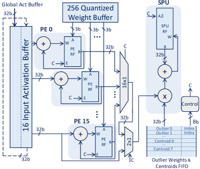
(a) Tile

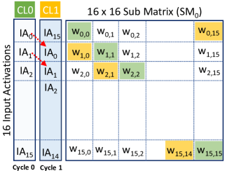
(b) Dataflow

Figure 6. GOBO Hardware Accelerator.

Tile Architecture: As Fig. 6a shows, each GOBO Tile contains a column of 16 Processing Elements (PEs). Each PE contains an FP32 adder and an 8-entry register file, one per possible weight index. The PE is designed to process 3b weight indexes (GOBO can combine tiles to process wider weight indexes). The 16 PEs are all connected to a single Shared Processing Unit (SPU) which has a 16-entry output activation register file, with one entry per PE. The SPU performs the final per centroid MAC operations and also handles the outliers. For this discussion, for clarity, we initially assume an output stationary dataflow where each output activation is produced by one only PE. We have experimented with several dataflows and we describe the one that we use in our experiments later on. Processing proceeds into two phases. In the first phase the PEs accumulate activations in their register files according to incoming “G” group weight indexes. In addition, the SPU is activated any time an outlier is encountered. In the second phase, the SPU processes the sums from each PE, one PE at a time, multiplies them with the centroids, and produces the final output activations.

Phase 1: Per index Activation Accumulation: At the unit’s front there are two circular 16-entry activation buffers. At any point, one buffer, the staging buffer, loads one activation at a time from the global buffer, while the PEs use the other, the current buffer. It takes 16 cycles for the staging buffer to fill, during which the current buffer rotates its entries so that each activation is seen by each PE. Let us ignore outlier processing for the time being. Every cycle, the quantized weight buffer provides 16 weight indexes, one per PE. The PEs use these weights to add the current activation to the corresponding register file entry. Figure 6b shows how processing proceeds. For example, in Cycle 0, PE0 uses $W_{0,0}$ to accumulate activation $\mathit{IA}_{0}$, while PE2 uses $W_{2,2}$ to accumulate activations $\mathit{IA}_{2}$. In cycle 1, the activations are rotated by one position, and now PE0 uses $W_{0,15}$ to appropriately accumulate activation $\mathit{IA}_{15}$. After 16 cycles, the first block of input activations completes processing, and staging and input buffers switch roles, so that processing can proceed with $\mathit{IA}_{16}$ through $IA_{31}$. The 16 weights along the diagonals in the SM of Figure 6b form a block in memory and are stored next to one another as in Figure 5c. Once all activations have been seen, we proceed to phase two.

Phase 2: Centroid Processing: This phase proceeds in centroid/PE order. As shown in Figure 6a, the centroid values are read from the global buffer one by one. Once centroid 0 is read, the SPU uses 16 cycles to multiply it with the corresponding PE register file entry from each PE writing the result into the SPU register file entry for the PE. Then, the SPU proceeds with centroid 1 and so on. In total it takes $8\times 16=128$ cycles to finish phase 2. During this time the PEs are idle. Recall that the FC layers are large so at the end this is a small overhead. GOBO will more than make up for this overhead by keeping more weights on-chip and by being able to use more PEs per unit area. If desired, adding more SPUs per tile would reduce this idle time.

Outlier Processing: Outliers are processed during phase 1 by the SPU. The SPU reads the outliers from the global buffer into a FIFO. Recall that the outliers are stored using the format of Figure 5c. Accordingly, the SPU determines the original positions of the outliers, as it encounters them in the order they should be processed according to the described dataflow. For the next outlier in order, the SPU disables accumulation in the corresponding PE when the dummy weight index appear. It then waits until the corresponding activation is rotated to appear at PE15. At that time the SPU can bypass it directly and multiply it with the outlier weight accumulating the result into the appropriate output register file entry (recall that outliers are to be used as-is, they are not mapped to centroids). At the same time PE15 can process the activation as required. If there are multiple outliers for an activation (the weight matrix has multiple outliers in the same column), the SPU will take as many cycles as needed to process them one by one. During those extra cycles, the PEs are disabled.

Finally, this organization can support 4b weight indexes so that we can execute models such as RoBERTa which require 4b dictionaries for some of their layers. To do so, we pair adjacent tiles so that the 8-entry register files in the first tile store the accumulation of input activations corresponding to the first 8 weight indexes, and the second tile stores the rest. The output register file entries have to be added in pairs to get the final output. This is done over 16 cycles reuse the adder from one of the tiles.

Memory Organization: A GOBO accelerator will typically have several tiles. A banked Global Buffer supplies the tiles with the data they need. The most demanding data needs are for the weight indexes. Each tile processes at peak one block of 16 weight indexes per cycle which requires $16\times 3b=48b$ per cycle. Each tile also reads a single FP32 activation per cycle at peak. However, the same activation can be shared among all tiles. Finally, each tile also needs to read in outliers which require at most 40b each plus an 8b count per submatrix of 256 weights. However, the outliers are infrequent and the bandwidth needs are low. Accordingly, we partition the Global Buffer across the tiles with at least three banks per tile. One for activations, one wider for weights, and finally one for the outliers plus centroids. Note that there is one set of centroids per layer that we replicate across tiles.

Dataflow: We have experimented with several dataflows and as previous work have found that the output stationary dataflow is not best (EyerissISCA2016, ). Instead of dedicating each PE to process one output activation at a time, we time multiplex over multiple subsets of activations (from multiple input words) producing partial sums. For this purpose, we block weights in groups of columns, and if beneficial rows, and process the corresponding activation columns producing partial sums. We perform phase 1 and phase 2 processing to produce these partial sums. This allows us to take advantage of weight reuse across words; we use the same weights with the corresponding activations for many words. Once done with all words for one group, we proceed with the next group of columns (and rows) of weights.

7. Evaluation

This section demonstrates the performance and energy-efficiency benefits when 1) GOBO is used to compress data off-chip, and 2) for an accelerator that uses GOBO compression and the GOBO processing architecture.

We use the models discussed in Section 2. The models are quantized with GOBO to 3b except for 12 layers of RoBERTa and 28 layers of RoBERTa-Large that are quantized to 4b as discussed in Section 4.3. Cycle times are measured using a custom cycle-accurate simulator which uses DRAMsim2 (DRAMsim2, ) to model off-chip transfers for a DDR4-3200 dual-channel DRAM main memory. The simulator has been tested extensively with microbenchmarks. The simulator computes values faithfully in time which it compares against the expected outputs for correctness. Area and power for the on-chip memories are modeled by CACTI (CACTI, ). Memories are divided into banks to meet the target access time and bandwidth. We use post-layout energy and area estimates: All designs are implemented in Verilog and synthesized using Synopsys’ Design Compiler (design_comp, ) with a 65nm TSMC technology library and a 1 GHz target frequency. Layouts are generated using Cadence Innovus (innovus, ). For power estimation, we use Intel ModelSim to generate signal activity as input to Innovus.

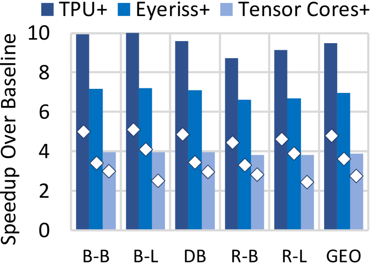
(a) GOBO Mem. Comp.: Speedup

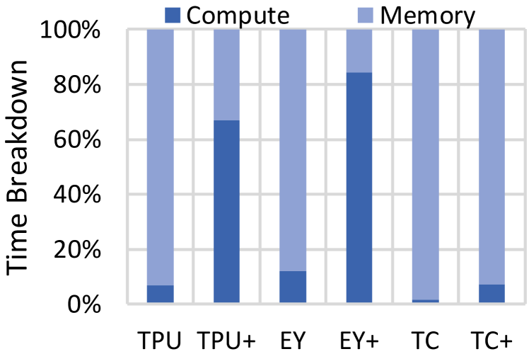
(b) GOBO Mem. Comp.: Time Breakdown

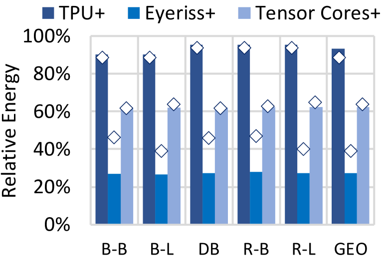
(c) GOBO Mem. Comp.: Relative Energy

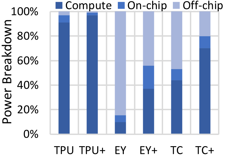
(d) GOBO Mem. Comp.: Energy Breakdown

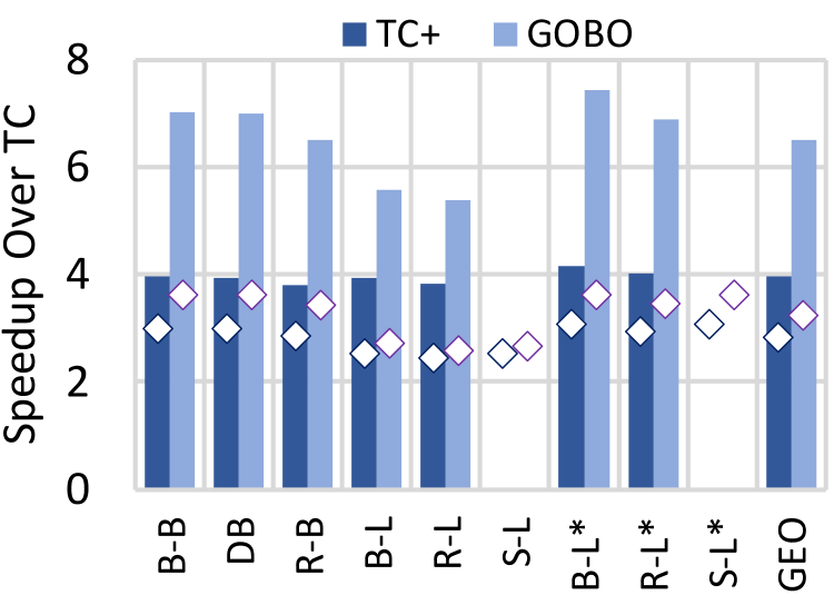
(e) GOBO Accelerator: Speedup over TC.

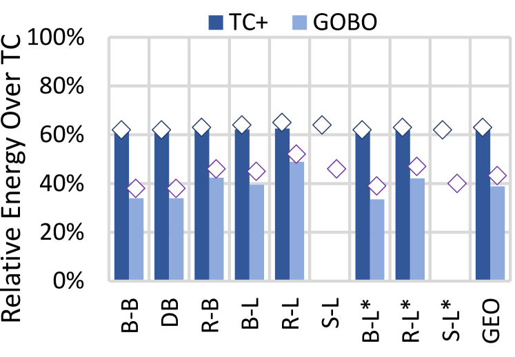
(f) GOBO Acc.: Relative Energy over TC.

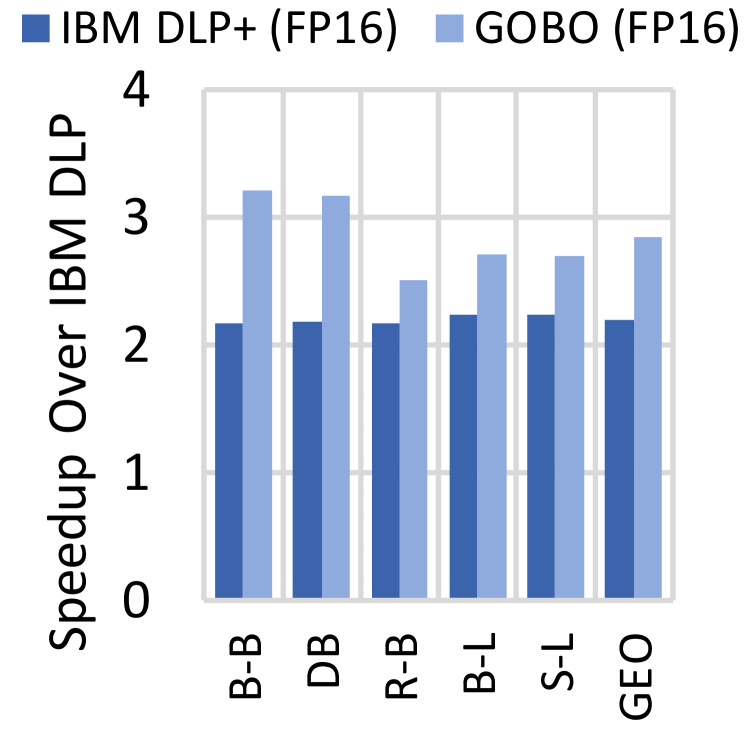
(g) Speedup: GOBO Vs. DLP

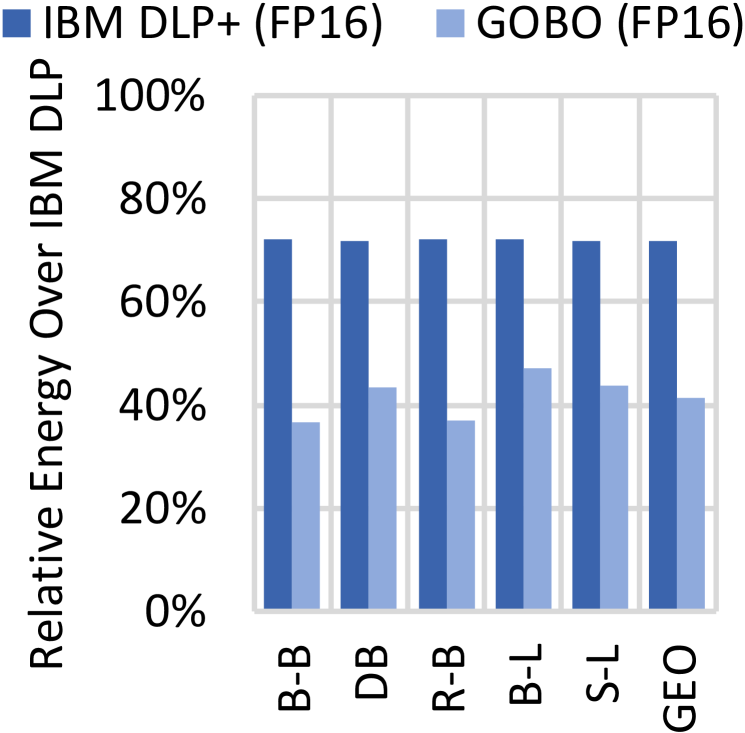
(h) Rel. E.: GOBO Vs. DLP

Figure 7. Evaluation of GOBO Memory Compression and Hardware Accelerator. In figures (a) to (f) bars show original FP32 models, and $\mathbf{\diamond}$ markers show scaled FP16 models. B-B, B-L, DB, R-B, R-L, and S-L are short for BERT-Base, BERT-Large, DistilBERT, RoBERTa-Base, RoBERTa-Large, and SpanBERT-Large respectively. B-L*, R-L*, and S-L* refer to BERT-Large, RoBERTa-Large, and SpanBERT-Large models on configurations of TC, TC+ and GOBO with a 4MB on-chip buffer for FP32, and a 2MB for FP16 architectures. EY and TC, stand for Eyeriss and Tensor Cores. TPU+, EY+, TC+, IBM DLP+ use GOBO off-chip memory compression. Fine-tuned FP32 version of SpanBERT was not available.

7.1. Memory Compression

We incorporate GOBO memory compression (Section 5) over three popular deep learning hardware architectures. TPU (TPUISCA17, ) and Eyeriss (EyerissISCA2016, ) are configured as originally presented. To execute these models, however, we implement them with FP32 and FP16 MAC units from a vendor provided library. The MAC units are optimized for energy efficiency. We configure the modeled Tensor Cores accelerator with 128 Tensor Core-like units  (TC1, ; TC2, ) and with a 2MB on-chip buffer. Each Tensor Core unit performs a $A_{4\times 4}\times B_{4\times 4}$ matrix multiply producing a matrix $C_{4\times 4}$ per cycle (GPGPU, ). It is configured to perform 64 MAC operations per cycle. We adjust the dataflow of each architecture to improve performance and energy efficiency.

Figure 7a reports speedups when we introduce GOBO memory compression. Speedups are measured over the corresponding architecture without GOBO. Note that these models are not sparse and use FP32 which makes zero compression or other compression methods targeting fixed-point neural networks inapplicable.

TPU: Performance for the TPU improves nearly by $10\times$. The TPU keeps all activations on-chip and reads weights from off-chip memory. For these networks the TPU is severely memory bound on the weight side thus benefiting fully from the traffic reduction possible with GOBO. Speedups are slightly lower for DistilBERT and the RoBERTa models. The size of the FC layers in DistilBERT leads to different utilization of the TPU’s systolic array, and as a result the potential for improvement from memory compression is different than it is for the BERT models. The RoBERTa models have layers that are quantized to 4b instead of 3b.

Eyeriss: Speedup on Eyeriss is at nearly $7\times$ on average. Eyeriss optimizes the dataflow to keep MACs busy, and has much fewer MACs than server-class accelerators such as the TPU. Accordingly, the potential for speedup is lower.

Tensor Cores: This architecture is also memory bound with $16\%$ of all memory transactions being for activations and partial sums, while weights account for the remaining $84\%$. Given that GOBO reduces weight footprint by nearly $10\times$, performance improves by nearly $4\times$.

Execution Time Breakdown: Figure 7b shows an execution time breakdown for each architecture. The configurations with GOBO memory compression are labeled as TPU+, EY+ (Eyeriss), and TC+ (Tensor Cores) and the graphs report averages over all networks. The measurements confirm that off-chip accesses account for most of the execution time in the baseline architectures. Using GOBO memory compression, the fraction of time taken by off-chip accesses is reduced to $32\%$ and $15\%$ for TPU+ and Eyeriss+ respectively. Off-chip accesses remain a major bottleneck for TC+ since the activations and the partial sums still require many off-chip accesses. Regardless, TC+ is $4\times$ faster than TC.

Energy: DRAM transactions are expensive in terms of time and energy. Figure 7c reports the energy reduction for each architecture with GOBO memory compression over the baseline. TPU, whose compute grid account for 90% of overall energ comsumption (Figure 7d), sees the least benefit of 7%. Energy consumption for Eyeriss improves on average by $3.7\times$ since computation only accounts for 10% of total energy. In Tensor Cores, off-chip memory accounts for 47% of total energy, which GOBO reduces to 20% improving overall energy consumption by $1.6\times$ on average.

FP16: Recent architectures add support for 16b floating-point as it has proven sufficient for training and inference of many neural networks. Figure 7a ($\diamond$ markers) reports speedups with GOBO compression assuming the models can use FP16 (presently only demonstrated with SpanBERT). All hardware architectures are configured to use FP16 for off-chip traffic and on-chip processing. GOBO compression proves effective throughout. Speedups compared to FP32 are halved for the TPU and Eyeriss where weights dominate off-chip traffic. FP16 is less effective for TC as about 16% of the off-chip traffic is for partial sums. Figure 7c ($\diamond$ markers) shows that the relative energy benefits with GOBO compression for the TPU and TC where most energy is consumed in the compute units. The relative benefits scale less for Eyeriss due to its small global buffer (off-chip traffic is more pronounced and using FP16 leaves less potential for compression). Still, even with FP16, GOBO compression reduces energy by $2.5\times$.

7.2. GOBO Hardware Accelerator

We perform an iso-compute-area comparison of the GOBO accelerator with Tensor Cores and IBM DLP (IBM2018, ) like architectures. For Tensor Cores we study both FP32 and FP16 variants, and for the IBM DLP we model FP16 hardware as originally proposed. We first focus on the FP32 comparison with Tensor Cores. Tensor Cores and GOBO FP32 designs are given the same 2MB on-chip memory. Table 12 summarizes the configurations. The FP32 Tensor Cores’ tile is $6.2\times$ larger than the GOBO tile while it has $4\times$ more multipliers and accumulators. Recall that GOBO replaces each multiplier with an accumulator and an 8-entry register file, and that there is only a single MAC unit that is shared across multiple PEs. Table 12 shows the GOBO tile area breakdown. An FP32 multiplier is $4.1\times$ larger than an 8-entry register file. As a result, for the same compute area needed by 128 Tensor Cores, we can fit 768 GOBO tiles.

Table 10. Tensor Cores & GOBO: Area.

	Tile Area $(mm^{2})$		Tiles/Chip	MAC/Tile	MAC/Chip
Tensor Cores FP32	$0.84$	1$\times$	128	64	1$\times$
GOBO FP32	$0.13$	0.16$\times$	768	16	1.5$\times$
Tensor Cores FP16	$0.27$	1$\times$	160	64	1$\times$
GOBO FP16	$0.05$	0.20$\times$	768	16	1.2$\times$

Table 11. GOBO FP32 Tile Area Breakdown

Component Area ($\mu m^{2}$)			Module Area ($\mu m^{2}$)		Area/Tile
FP32 Adder	4,149	1$\times$	PE	6,780	80.02%
FP32 Multiplier	9,379	2.26$\times$	SPU	17,883	13.19%
PE Reg File (8x32)	2,628	0.63$\times$	Buffers	8,046	5.94%
SPU Reg File (16x32)	4,630	1.12$\times$

Table 12. Tensor Cores & GOBO: Absolute Perf. & Energy.

	Peak TFLOPS		BERT-Base (MNLI)
			Cycles (M)		Energy (J)
Architecture	FP32	FP16	FP32	FP16	FP32	FP16
TC	16	20	70.2	35.3	0.24	0.11
TC+	16	20	17.8	11.8	0.15	0.07
GOBO	24	24	9.9	9.7	0.08	0.04

Performance: Figure 7e reports the performance of GOBO relative to the baseline Tensor Cores (TC) and the Tensor Cores with GOBO off-chip compression (TC+). In this configuration, TC+ is about $4\times$ faster than TC across all models. GOBO is $7\times$ faster than TC for BERT-base and DistilBERT. Speedups with GOBO are slightly lower for RoBERTa as peak throughput is halved for those layers that are quantized to 4 bits. There are two primary reasons why GOBO improves performance. First, it has a higher peak compute throughput than TC as it can afford to pack more compute units for the same area. Second, it better utilizes the on-chip memory buffers as it keeps weights encoded throughout. GOBO’s speedup over TC on the large models caps at $5.5\times$ due to size of the on-chip buffer. To show how performance would scale with a larger on chip buffer we evaluated BERT-Large (B-L*) and RoBERTa-Large (R-L*) with TC, TC+ and GOBO configurations using a 4MB on-chip buffer. As expected, this results in higher speedups.

Energy: Relative energy trends in Figure 7f follow those of performance closely. For example, GOBO consumes $3\times$ less energy than TC on BERT-base and DistilBERT. Compute accounts for a large portion of TC, so avoiding FP32 multiplications greatly improves energy consumption. Table 12 reports absolute performance and energy for BERT-Base on TC, TC+ and GOBO. Overall, GOBO is $21\times$ more energy efficient than TC.

FP16: We scale the FP32 configurations to use FP16 instead. Table 12 reports the configurations when both TC and GOBO use FP16 units and a 1MB on-chip buffer. Given the non-linear scaling of FP multipliers, the ratio of TC to GOBO tiles decreases from $6.2\times$ to $5\times$. We keep the same number of GOBO tiles and increase the TC tiles so that both use the same compute area. Figure 7e ($\diamond$ markers) shows the relative performance of FP16 TC+ (uses GOBO compression) and GOBO over FP16 TC. GOBO compression makes TC+ $2.8\times$ faster than TC and the GOBO accelerator is even faster at $3.3\times$. Moreover, GOBO remains the most energy efficient architecture of the three. Figure 7f reports that GOBO consumes $2.4\times$ less energy compared to TC. Using just GOBO compression improves TC+’s energy over TC by $1.6\times$. Table 12 reports absolute performance and energy for these FP16 configurations.

IBM DLP: IBM’s Deep learning Processor (IBM2018, ) is an FP16 systolic array with a 2MB on-chip buffer. We demonstrate that a) IBM DLP benefits from GOBO memory compression (IBM DLP+), and b) under iso-compute-area constraints GOBO accelerator is higher performing and more energy efficient. We configure DLP’s systolic array with 512 MACs to match the 1K FLOPS/cycle originally reported. GOBO’s tiles are $1.2\times$ smaller than DLP’s allowing us to fit 20% more tiles. GOBO is configured with the same 2MB on-chip capacity. Figures 7g and 7h report GOBO Accelerator’s and IBM DLP+’s performance and relative energy over the IBM DLP baseline. GOBO memory compression increases PE utilization from 34% to 75% in DLP+, making it $2.2\times$ faster, whereas GOBO is even faster at $2.85\times$ as its PE utilization is 83%. GOBO is the most energy efficient: $2.4\times$ vs. DLP+ and $6.8\times$ vs the original DLP.

8. Conclusion

We presented a post-training quantization method for attention-based NLP models. We demonstrated that it can significantly reduce model size (parameters and embedding tables) with little or no effect on accuracy. We presented two practical applications. In the first, which is plug-in compatible with other accelerators, GOBO is used to compress data from off-chip boosting energy efficiency and off-chip capacity. In the second, we presented an accelerator that uses GOBO quantization throughout. It is unique in that it never expands the weights into their original values directly.

References

- (1) J. Devlin, M.-W. Chang, K. Lee, and K. Toutanova, “Bert: Pre-training of deep bidirectional transformers for language understanding,” in NAACL-HLT, 2019.
- (2) V. Sanh, L. Debut, J. Chaumond, and T. Wolf, “Distilbert, a distilled version of bert: smaller, faster, cheaper and lighter,” 5th Workshop on Energy Efficient Machine Learning and Cognitive Computing - NeurIPS, 2019.
- (3) S. Shen, Z. Dong, J. Ye, L. Ma, Z. Yao, A. Gholami, M. W. Mahoney, and K. Keutzer, “Q-bert: Hessian based ultra low precision quantization of bert.” in AAAI, 2020, pp. 8815–8821.
- (4) O. Zafrir, G. Boudoukh, P. Izsak, and M. Wasserblat, “Q8bert: Quantized 8bit bert,” 5th Workshop on Energy Efficient Machine Learning and Cognitive Computing - NeurIPS, 2019.
- (5) S. Han, H. Mao, and W. J. Dally, “Deep compression: Compressing deep neural network with pruning, trained quantization and huffman coding,” in 4th International Conference on Learning Representations, ICLR 2016, San Juan, Puerto Rico, May 2-4, 2016, Conference Track Proceedings, Y. Bengio and Y. LeCun, Eds., 2016. [Online]. Available: http://arxiv.org/abs/1510.00149
- (6) S. Han, X. Liu, H. Mao, J. Pu, A. Pedram, M. A. Horowitz, and W. J. Dally, “Eie: Efficient inference engine on compressed deep neural network,” in Proceedings of the 43rd International Symposium on Computer Architecture, ser. ISCA ’16. IEEE Press, 2016, p. 243–254. [Online]. Available: https://doi.org/10.1109/ISCA.2016.30
- (7) E. Park, S. Yoo, and P. Vajda, “Value-aware quantization for training and inference of neural networks,” in Proceedings of the European Conference on Computer Vision (ECCV), 2018, pp. 580–595.
- (8) E. Park, D. Kim, and S. Yoo, Energy-Efficient Neural Network Accelerator Based on Outlier-Aware Low-Precision Computation. IEEE Press, 2018, p. 688–698. [Online]. Available: https://doi.org/10.1109/ISCA.2018.00063
- (9) J. Fang, A. Shafiee, H. Abdel-Aziz, D. Thorsley, G. Georgiadis, and J. Hassoun, “Post-training piecewise linear quantization for deep neural networks,” 2020.
- (10) Y. Liu, M. Ott, N. Goyal, J. Du, M. Joshi, D. Chen, O. Levy, M. Lewis, L. Zettlemoyer, and V. Stoyanov, “Roberta: A robustly optimized bert pretraining approach,” arXiv preprint arXiv:1907.11692, 2019.
- (11) H. Wang, Z. Wu, Z. Liu, H. Cai, L. Zhu, C. Gan, and S. Han, “HAT: Hardware-aware transformers for efficient natural language processing,” in Proceedings of the 58th Annual Meeting of the Association for Computational Linguistics. Online: Association for Computational Linguistics, Jul. 2020, pp. 7675–7688. [Online]. Available: https://www.aclweb.org/anthology/2020.acl-main.686
- (12) M. Joshi, D. Chen, Y. Liu, D. S. Weld, L. Zettlemoyer, and O. Levy, “Spanbert: Improving pre-training by representing and predicting spans,” Transactions of the Association for Computational Linguistics, vol. 8, pp. 64–77, 2020.
- (13) A. Wang, A. Singh, J. Michael, F. Hill, O. Levy, and S. R. Bowman, “GLUE: A multi-task benchmark and analysis platform for natural language understanding,” in 7th International Conference on Learning Representations, ICLR 2019, New Orleans, LA, USA, May 6-9, 2019. OpenReview.net, 2019. [Online]. Available: https://openreview.net/forum?id=rJ4km2R5t7
- (14) S. Narasimhan, “Nvidia developer blog,” Aug 2019. [Online]. Available: https://devblogs.nvidia.com/training-bert-with-gpus]/
- (15) P. Rajpurkar, J. Zhang, K. Lopyrev, and P. Liang, “Squad: 100,000+ questions for machine comprehension of text,” arXiv preprint arXiv:1606.05250, 2016.
- (16) P. Ganesh, Y. Chen, X. Lou, M. A. Khan, Y. Yang, D. Chen, M. Winslett, H. Sajjad, and P. Nakov, “Compressing large-scale transformer-based models: A case study on bert,” arXiv preprint arXiv:2002.11985, 2020.
- (17) E. Wang, J. J. Davis, R. Zhao, H.-C. Ng, X. Niu, W. Luk, P. Y. K. Cheung, and G. A. Constantinides, “Deep neural network approximation for custom hardware,” ACM Computing Surveys, vol. 52, no. 2, p. 1–39, May 2019. [Online]. Available: http://dx.doi.org/10.1145/3309551
- (18) S. Shi, X. Chu, K. C. Cheung, and S. See, “Understanding top-k sparsification in distributed deep learning,” arXiv preprint arXiv:1911.08772, 2019.
- (19) M. A. Gordon, K. Duh, and N. Andrews, “Compressing bert: Studying the effects of weight pruning on transfer learning,” arXiv preprint arXiv:2002.08307, 2020.
- (20) O. Kovaleva, A. Romanov, A. Rogers, and A. Rumshisky, “Revealing the dark secrets of bert,” arXiv preprint arXiv:1908.08593, 2019.
- (21) A. Raganato, Y. Scherrer, and J. Tiedemann, “Fixed encoder self-attention patterns in transformer-based machine translation,” arXiv preprint arXiv:2002.10260, 2020.
- (22) A. Fan, E. Grave, and A. Joulin, “Reducing transformer depth on demand with structured dropout,” CoRR, vol. abs/1909.11556, 2019. [Online]. Available: http://arxiv.org/abs/1909.11556
- (23) S. Zhao, R. Gupta, Y. Song, and D. Zhou, “Extreme language model compression with optimal subwords and shared projections,” arXiv preprint arXiv:1909.11687, 2019.
- (24) Z. Sun, H. Yu, X. Song, R. Liu, Y. Yang, and D. Zhou, “Mobilebert: a compact task-agnostic BERT for resource-limited devices,” CoRR, vol. abs/2004.02984, 2020. [Online]. Available: https://arxiv.org/abs/2004.02984
- (25) X. Jiao, Y. Yin, L. Shang, X. Jiang, X. Chen, L. Li, F. Wang, and Q. Liu, “Tinybert: Distilling BERT for natural language understanding,” CoRR, vol. abs/1909.10351, 2019. [Online]. Available: http://arxiv.org/abs/1909.10351
- (26) S. Sun, Y. Cheng, Z. Gan, and J. Liu, “Patient knowledge distillation for bert model compression,” arXiv preprint arXiv:1908.09355, 2019.
- (27) Y. Cheng, D. Wang, P. Zhou, and T. Zhang, “A survey of model compression and acceleration for deep neural networks,” 2017.
- (28) R. Tang, Y. Lu, L. Liu, L. Mou, O. Vechtomova, and J. Lin, “Distilling task-specific knowledge from bert into simple neural networks,” arXiv preprint arXiv:1903.12136, 2019.
- (29) R. Tang, Y. Lu, and J. Lin, “Natural language generation for effective knowledge distillation,” in Proceedings of the 2nd Workshop on Deep Learning Approaches for Low-Resource NLP (DeepLo 2019), 2019, pp. 202–208.
- (30) Y. K. Chia, S. Witteveen, and M. Andrews, “Transformer to cnn: Label-scarce distillation for efficient text classification,” arXiv preprint arXiv:1909.03508, 2019.
- (31) T. Wolf, L. Debut, V. Sanh, J. Chaumond, C. Delangue, A. Moi, P. Cistac, T. Rault, R. Louf, M. Funtowicz, and J. Brew, “Huggingface’s transformers: State-of-the-art natural language processing,” ArXiv, vol. abs/1910.03771, 2019.
- (32) Y.-H. Chen, J. Emer, and V. Sze, “Eyeriss: A spatial architecture for energy-efficient dataflow for convolutional neural networks,” in Intl’ Symp. on Computer Architecture, 2016.
- (33) P. Rosenfeld, E. Cooper-Balis, and B. Jacob, “Dramsim2: A cycle accurate memory system simulator,” IEEE Computer Architecture Letters, vol. 10, no. 1, pp. 16–19, Jan 2011.
- (34) N. Muralimanohar, R. Balasubramonian, and N. Jouppi, “Cacti 6.0: A tool to model large caches,” HP Laboratories, 01 2009.
- (35) Synopsys, “Design compiler graphical,” https://www.synopsys.com/implementation-and-signoff/rtl-synthesis-test/design-compiler-graphical.html.
- (36) Cadence, “Innovus implementation system,” https://www.cadence.com/content/cadence-www/global/en_US/home/tools/digital-design-and-signoff/hierarchical-design-and-floorplanning/innovus-implementation-system.html.
- (37) N. P. Jouppi, C. Young, N. Patil, D. Patterson, G. Agrawal, R. Bajwa, S. Bates, S. Bhatia, N. Boden, A. Borchers, R. Boyle, P.-l. Cantin, C. Chao, C. Clark, J. Coriell, M. Daley, M. Dau, J. Dean, B. Gelb, T. V. Ghaemmaghami, R. Gottipati, W. Gulland, R. Hagmann, C. R. Ho, D. Hogberg, J. Hu, R. Hundt, D. Hurt, J. Ibarz, A. Jaffey, A. Jaworski, A. Kaplan, H. Khaitan, D. Killebrew, A. Koch, N. Kumar, S. Lacy, J. Laudon, J. Law, D. Le, C. Leary, Z. Liu, K. Lucke, A. Lundin, G. MacKean, A. Maggiore, M. Mahony, K. Miller, R. Nagarajan, R. Narayanaswami, R. Ni, K. Nix, T. Norrie, M. Omernick, N. Penukonda, A. Phelps, J. Ross, M. Ross, A. Salek, E. Samadiani, C. Severn, G. Sizikov, M. Snelham, J. Souter, D. Steinberg, A. Swing, M. Tan, G. Thorson, B. Tian, H. Toma, E. Tuttle, V. Vasudevan, R. Walter, W. Wang, E. Wilcox, and D. H. Yoon, “In-datacenter performance analysis of a tensor processing unit,” in International Symposium on Computer Architecture, 2017.
- (38) Z. Jia, M. Maggioni, B. Staiger, and D. P. Scarpazza, “Dissecting the NVIDIA volta GPU architecture via microbenchmarking,” CoRR, vol. abs/1804.06826, 2018. [Online]. Available: http://arxiv.org/abs/1804.06826
- (39) L. Durant, O. Giroux, M. Harris, and N. Stam, “Nvidia developer blog,” May 2017. [Online]. Available: https://devblogs.nvidia.com/inside-volta/
- (40) M. A. Raihan, N. Goli, and T. M. Aamodt, “Modeling deep learning accelerator enabled gpus,” in 2019 IEEE International Symposium on Performance Analysis of Systems and Software (ISPASS), 2019, pp. 79–92.
- (41) B. Fleischer, S. Shukla, M. Ziegler, J. Silberman, J. Oh, V. Srinivasan, J. Choi, S. Mueller, A. Agrawal, T. Babinsky, N. Cao, C. Chen, P. Chuang, T. Fox, G. Gristede, M. Guillorn, H. Haynie, M. Klaiber, D. Lee, S. Lo, G. Maier, M. Scheuermann, S. Venkataramani, C. Vezyrtzis, N. Wang, F. Yee, C. Zhou, P. Lu, B. Curran, L. Chang, and K. Gopalakrishnan, “A scalable multi- teraops deep learning processor core for ai training and inference,” in 2018 IEEE Symposium on VLSI Circuits, 2018, pp. 35–36.