Apparent superballistic dynamics in one-dimensional random walks with biased detachment

Abstract

The mean-squared displacement (MSD) is an averaged quantity widely used to assess anomalous diffusion. In many cases, such as molecular motors with finite processivity, dynamics of the system of interest produce trajectories of varying duration. Here we explore the effects of finite processivity on different measures of the MSD. We do so by investigating a deceptively simple dynamical system: a one-dimensional random walk (with equidistant jump lengths, symmetric move probabilities, and constant step duration) with an origin-directed detachment bias. By tuning the time dependence of the detachment bias, we find through analytical calculations and trajectory simulations that the system can exhibit a broad range of anomalous diffusion, extending beyond conventional diffusion to superdiffusion and even superballistic motion. We analytically determine that protocols with a time-increasing detachment lead to an ensemble-averaged velocity increasing in time, thereby providing the effective acceleration that is required to push the system above the ballistic threshold. MSD analysis of burnt-bridges ratchets similarly reveals superballistic behavior. Because superdiffusive MSDs are often used to infer biased, motor-like dynamics, these findings provide a cautionary tale for dynamical interpretation.

I Introduction

The mean-squared displacement (MSD) is often used to assess anomalous diffusion in molecular systems. A system with an MSD that grows linearly in time is conventionally diffusive, lacking anomalous effects Einstein (1956):

$${\mathrm{MSD}=\left\langle x^{2}(t)\right\rangle=2Dt.}$$ (1)

For processes that obey (1), such as a discrete-time random walk, the displacement distribution after $N$ steps limits to a Gaussian distribution. That is, the $N$ individual steps of a discrete-time random walk are independent and identically distributed, with their sum governed by the central limit theorem Metzler and Klafter (2000).

Anomalous diffusion refers to systems that do not have a linear time dependence of the MSD. Generally, anomalous diffusion is thought to emerge in stochastic systems whose displacement distributions are not Gaussian, and is therefore intimately connected with the breakdown of the central limit theorem Metzler and Klafter (2000). The concept of anomalous diffusion was first introduced in 1926 by L.F. Richardson Richardson (1926) through a thought experiment involving two independent air particles separated by a sufficiently large distance so as to be caught by two independent gusts of wind moving in opposite directions. Richardson hypothesized that such a system does not obey Fick’s second law, and that the MSD of the air particles scales nonlinearly with time. For an anomalously diffusive system,

$$\mathrm{MSD}\propto D_{\rm g}t^{\alpha}\ ,$$ (2)

where $D_{\rm g}$ is the generalized diffusion coefficient, and $\alpha$ is the anomalous diffusion exponent that distinguishes the type of diffusion Havlin and Ben-Avraham (2002); Metzler and Klafter (2000); Metzler et al. (2014). Subdiffusion, conventional diffusion, and superdiffusion correspond to $0\leq\alpha<1$, $\alpha=1$, and $1<\alpha<2$, respectively. The ballistic threshold is at $\alpha=2$, describing a system whose trajectories proceed at constant velocity.

In order for a microscopic system to behave ballistically over long times an external stimulus is typically required. For example, ballistic motion is achieved for random walkers subject to certain forms of external noise Bao and Zhuo (2003). Ballistic motion can also be achieved without an external stimulus in systems whose cooperative behavior limits the degrees of freedom of individual particles Feinerman et al. (2018); Rank et al. (2013). To exceed $\alpha=2$, reaching the superballistic regime, it is generally thought an acceleration is required ben-Avraham et al. (1992). Examples include animal movement generated by muscle contraction Tilles et al. (2017) and particles optically trapped in air Li et al. (2010); Duplat et al. (2013), subject to increasing temperatures Cherstvy and Metzler (2016), or subject to expanding media Le Vot et al. (2017).

In this work we consider a deceptively simple one-dimensional discrete random walk with equal-sized and equal-duration steps. We impose no external forces, particle thrust, noise typically thought to promote superdiffusive motion, or cooperative behavior. We instead impose a tunable detachment probability $d$ that produces finite processivity. For every step toward its initial position, the random walker permanently detaches with probability $d$. We explore two detachment protocols: constant detachment, and detachment exponentially increasing at rate $k_{\rm d}$.

By varying $d$ or $k_{\rm d}$, we find that the anomalous diffusion exponent $\alpha$ can be tuned over a wide range of values. Varying $d$ controls apparent time-dependent dynamics ranging from diffusive to ballistic, while variations in $k_{\rm d}$ tune $\alpha$ from the diffusive into a transient but long-lasting superballistic regime. We determine the mechanism for this apparently superballistic behavior by analytically deriving the ensemble velocity and find it is dependent on the detachment protocol used, thereby producing the ensemble acceleration required to breach the ballistic threshold. We reproduce several of these observations in a trajectory-resolved model, though find that distinct approaches to calculating the MSD provide different values of $\alpha$ and hence distinct inferences about the system’s dynamics. We additionally show that selecting a subset of especially processive trajectories—as is common in single-particle studies Salman et al. (2002); Howse et al. (2007); Manley et al. (2008)—can introduce a large superdiffusive bias into the MSD. As an example, we demonstrate that this acceleration-by-detachment can manifest in a more realistic system by calculating MSD for burnt-bridges ratchets, which we find to exhibit apparently superballistic behavior. Our results encourage increased transparency regarding selection methods for single-particle analysis.

II Modeling random walks with detachment

II.1 Ensemble-level model

First we study a discrete-time diffusion scheme where we track the probability flow of an ensemble of independent one-dimensional random walkers. At time intervals $\Delta t=1$, each walker moves a distance $\Delta x=1$, with equal probability of going left or right. A step towards the initial position at the origin incurs a probability of detachment, either with constant or with exponential probability. For constant detachment, the probability $d$ of detaching is independent of time. Exponential detachment probability is given by

$$d(t)=1-e^{-k_{\rm d}t}\ ,$$ (3)

increasing over time as determined by the rate $k_{\rm d}$. (Thus the probability of remaining attached at each origin-directed step is $r(t)=1-d(t)$.) Detachment events of individual walkers are independent. Table 1 shows such a system’s initial evolution. For the results shown in this work, the probability distribution was evolved for $n=1000$ timesteps.

Table 1: Probability distributions for the first 4 time steps of the ensemble-level model.

		Displacement
		-4	-3	-2	-1	0	1	2	3	4
Time	0					1
	1				$\frac{1}{2}$	0	$\frac{1}{2}$
	2			$\frac{1}{4}$	0	$\frac{1}{2}r$	0	$\frac{1}{4}$
	3		$\frac{1}{8}$	0	$\frac{3}{8}r$	0	$\frac{3}{8}r$	0	$\frac{1}{8}$
	4	$\frac{1}{16}$	0	$\frac{1}{4}r$	0	$\frac{3}{8}r^{2}$	0	$\frac{1}{4}r$	0	$\frac{1}{16}$

II.2 Trajectory-resolved model

We model a one-dimensional discrete-time random walk by sampling step lengths from a Gaussian distribution with zero mean and unit standard deviation. Steps toward the origin lead to detachment with probability described by (3). As a control, we compare to a random walk with no detachment, which produces conventional diffusion.

III Analysis Methods

III.1 Mean-squared displacement and $\alpha(t)$ for ensemble-level model

We define the MSD for the ensemble-level model as

$$\mathrm{MSD_{\rm EA}}=\left\langle x^{2}\right\rangle_{\rm rem}\equiv\frac{\sum p_{i}x_{i}^{2}}{P_{\rm rem}},$$ (4)

where $x_{i}$ is the $i^{\rm th}$ position, $p_{i}$ is the probability of having a walker at the $i^{\rm th}$ site, and $P_{\rm rem}$ is the total remaining probability. MSD_EA denotes an ensemble-averaged MSD, discussed more in the following sub-section.

The time dependence of the anomalous diffusion exponent $\alpha$ is sometimes calculated through a quantity called either the dynamic functional Kepten et al. (2013) or the local MSD scaling exponent Ghosh et al. (2016), which is the derivative of the logarithm of the MSD with respect to the logarithm of time Karmakar et al. (2016).

$$\alpha_{\psi}\equiv\frac{\mathrm{d(\log MSD)}}{\mathrm{d}(\log\Delta t)}\ .$$ (5)

It has been noted that the numerical derivative of (5) can become especially noisy at long times because of compression of linear sampling by logarithmic scaling, thereby introducing uncertainty into estimates of the time dependence of $\alpha$ Martin et al. (2002).

Alternatively, we introduce a two-point estimator $\alpha^{n}_{n-b}$ for $\alpha$ using timepoints $n$ and $n-b$. In one dimension and for no average drift ($\left\langle x\right\rangle=0$),

$$\alpha^{n}_{n-b}\equiv\log_{n}\left(\frac{\left\langle x^{2}(n)\right\rangle}{\left\langle x^{2}(n-b)\right\rangle}\right)\left(1-\frac{1}{\log_{n-b}n}\right)^{-1}\ .$$ (6)

(Appendix A provides a general derivation.) To the best of our knowledge, (6) has not been used before, and we find it useful for characterizing transient anomalous diffusion with the MSD. It is important to note that $b$ must be kept small in order to extract information about the local slope; for this reason we use $b=2$ in this work when estimating the time dependence of $\alpha$ with (6).

As an example of its utility, in Appendix B we compare $\alpha^{n}_{n-b}$ to $\alpha_{\psi}$ when the MSD undergoes an abrupt change in slope. Figure 8 shows that the numerical derivative from (5) produces a noisy approximation to $\alpha_{\psi}$, whereas $\alpha^{n}_{n-b}$ (6) is smooth throughout.

Table 2 in Appendix C presents $P_{\rm rem}$, $\sum p_{i}x_{i}^{2}$, $\left\langle x^{2}\right\rangle_{\rm rem}$, and $\alpha^{n}_{n-2}$ for the first 4 timesteps.

III.2 Mean-squared displacement and $\alpha(t)$ for trajectory-resolved model

There are many ways to compute the MSD of trajectories; we start by defining the squared displacement as

$$\Delta x_{j}^{2}\left(t,\tau\right)\equiv\left[x_{j}(t+\tau)-x_{j}(t)\right]^{2}\ ,$$ (7)

where $x_{j}$ denotes the position of the $j$th trajectory, $t$ is time, and $\tau$ is the time lag. The mean-squared displacement for an ensemble of $N$ independent walkers is

$$\left\langle{\Delta x^{2}\left(t,\tau\right)}\right\rangle\equiv\frac{1}{N}\sum_{j=1}^{N}\Delta x_{j}^{2}\left(t,\tau\right)\ .$$ (8)

We define the ensemble-averaged (EA) MSD as the MSD at time $\tau$, relative to the initial time zero:

$$\mathrm{MSD_{\rm EA}}\equiv\left\langle{\Delta x^{2}\left(0,\tau\right)}\right\rangle=\frac{1}{N}\sum_{j=1}^{N}\Delta x_{j}^{2}\left(0,\tau\right)\ .$$ (9)

This is equivalent to (4), above. By contrast, the trajectory-averaged (TA) MSD is computed independently for each trajectory,

$$\mathrm{MSD_{\rm TA}}\equiv\overline{\Delta x_{j}^{2}\left(\tau\right)}=\frac{\Delta t}{T_{j}-\tau+\Delta t}\sum_{t=0}^{T_{j}-\tau}\Delta x_{j}^{2}\left(t,\tau\right)\ ,$$ (10)

where $T_{j}$ is the total duration of the $j$th trajectory, and $\Delta t=1$ is the time step.

The van Hove correlation function or displacement distribution $G(x,\tau)$ collects all the displacements for a particular time lag $\tau$ across all the observed trajectories van Hove (1954); Akcasu et al. (1970); Ghosh et al. (2016). $G(x,\tau)$ describes the probability of a particular displacement for a time lag $\tau$. The variance of $G(x,\tau)$ is the ensemble MSD_TA (i.e., the MSD_ETA) for $\tau$:

$$\mathrm{MSD_{\rm ETA}}\equiv\left\langle\overline{\Delta x^{2}\left(\tau\right)}\right\rangle=\frac{1}{N}\sum_{j=1}^{N}\overline{\Delta x_{j}^{2}\left(\tau\right)}\ .$$ (11)

The MSD_ETA is particularly useful for many independent but short trajectories.

MSDs calculated from equations (9), (10), and (11) are asymptotically equal for an ergodic process: the time average converges to the ensemble average at a sufficiently long time. By contrast, differing MSDs may imply nonergodicity; examples of such systems include tracer particles in mucus Cherstvy et al. (2019) and a continuous-time random walk with diverging average waiting times Bel and Barkai (2005).

Here, we estimate $\alpha$ through a linear fit of log MSD as a function of log time. For visual aid we fit over local regions of approximate linearity and report the range of times used in the fit. Because this logarithmic scaling produces a non-normal distribution of errors, we use a generalized least squares (GLS) approach to estimate $\alpha_{\rm GLS}$ from the MSD Orsini and Greenland (2009), employing the function gls from the R library nlme.

III.3 Shape of probability distributions

Deviation of the displacement distribution $G(x,\tau)$ from a Gaussian can be quantified by the standardized fourth moment (the kurtosis),

$$\beta_{2}(x)\equiv\frac{\left\langle(x-\left\langle x\right\rangle)^{4}\right\rangle}{(\left\langle(x-\left\langle x\right\rangle)^{2}\right\rangle)^{2}}\ .$$ (12)

As a Gaussian distribution has $\beta_{2}(x)=3$, it is convenient to define the excess kurtosis $\gamma_{2}\equiv\beta_{2}-3$, such that any non-zero $\gamma_{2}$ indicates non-Gaussian behavior Rahman (1964); Kob and Andersen (1995).

IV Results & Discussion

IV.1 Ensemble-level analysis

We first determine the effects of a constant origin-directed detachment bias on the ensemble-level system. Figure 1a displays the evolution of the displacement distribution for the ensemble-level analysis with constant-detachment probability $d=0.4$. Two peaks form, symmetric about the origin, and move with increasing dispersion in the $\pm\hat{x}$ directions, respectively. This is expected, as steps towards the origin have a probability of detachment, whereas steps away from the origin do not. Figure 1b shows that as the probability $d$ of detachment increases, the probability of remaining on the track decays more rapidly. The MSD_EA (4) varies with $d$, ranging from a ballistic trend ($\alpha=2$) for detachment probability $d=1$ to conventional diffusion ($\alpha=1$) for the no-detachment scenario ($d=0$) (Fig. 1c). For intermediate $d$ ($0<d<1$), the MSD displays increasing superdiffusive trends with increasing $d$.

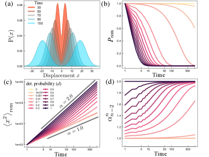
Figure 1: Ensemble-level analysis with constant detachment. (a) Evolution of the displacement distribution for constant-detachment probability $d=0.4$. (b) Probability of remaining on the track as a function of time, for different detachment probabilities $d$. (c) MSD_EA (4) as a function of time. (d) Diffusion exponent $\alpha^{n}_{n-b}$ (6) as a function of time. For $d=0$ (no detachment), $\alpha^{n}_{n-2}=1$ (conventional diffusion) at all times. As the detachment probability increases to $d=1$, $\alpha^{n}_{n-2}$ increases to the ballistic limit of 2.

To more quantitatively extract the time dependence of the anomalous diffusion exponent, we calculate $\alpha^{n}_{n-2}$ using (6). For all intermediate values of $d$, Fig. 1d shows that $\alpha$ increases with time monotonically towards the ballistic threshold; the transition to the ballistic threshold occurs sooner as $d\rightarrow 1$.

Figure 2 shows the ensemble-level analysis with an exponential time-dependent detachment probability given by (3). $d(t)$ is still bounded by $[0,1]$, but increases monotonically with time towards unity at a rate governed by $k_{\rm d}$ (Fig. 2a). The slowest detachment process studied, corresponding to $k_{\rm d}=10^{-2}$, leads to the slowest decay of $P_{\rm rem}$ from 1 to 0 (Fig. 2b). For the fastest detachment process studied ($k_{\rm d}=10^{4}$), the MSD_EA (4) appears ballistic at all times (Fig. 2c). As $k_{\rm d}$ decreases, the MSD transitions from diffusive to ballistic, exhibiting a long superballistic transient at intermediate times (peaking at $\alpha\approx 3.5$ for $k_{\rm d}=10^{-2}$). We find that all $k_{\rm d}<1$ lead to $\alpha^{n}_{n-2}$ rising past the ballistic threshold. This behavior is characterized in Fig. 2d, in which is is clear that as $k_{\rm d}$ decreases, the maximum $\alpha^{n}_{n-2}$ ($\alpha_{\rm max}$) increases further into the superballistic regime. Figure 2e shows that $\alpha_{\rm max}$ decreases from strongly superballistic as $k_{\rm d}$ increases, until for $k_{\rm d}>1$, $\alpha^{n}_{n-b}$ reaches and remains near the ballistic limit. Figure 2f shows that $\alpha_{\rm max}$ occurs later as $k_{\rm d}$ increases. Therefore, as the origin-biased detachment process is slowed, the system takes longer to breach the ballistic threshold, but extends farther into the superballistic regime and stays superballistic for longer.

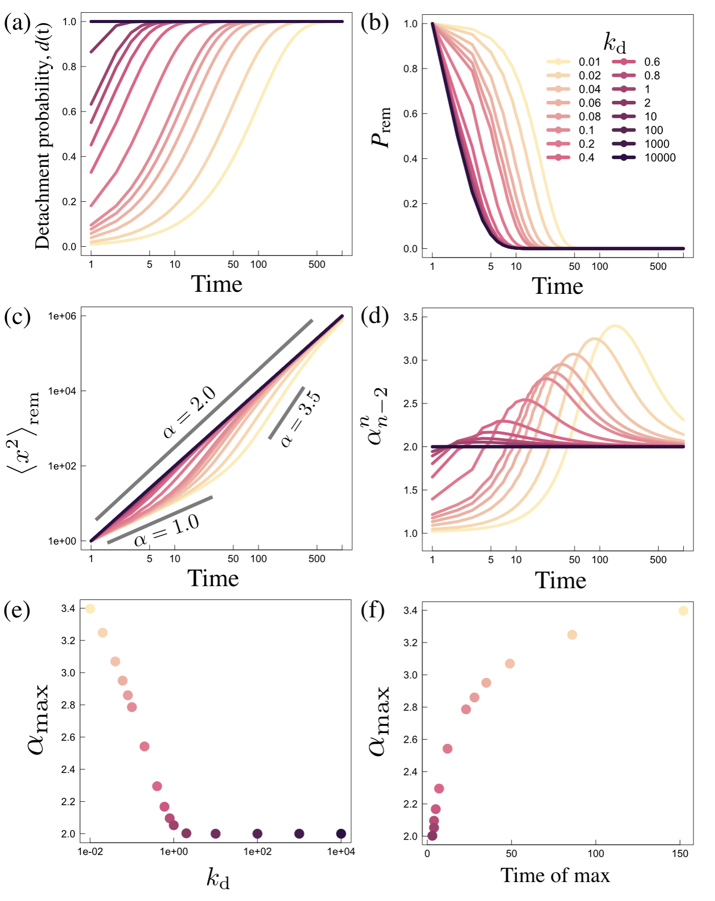
Figure 2: Ensemble-level analysis with exponential detachment. (a) Time-dependent detachment probability (3) as a function of time for various decay rates $k_{\rm d}$. (b) Probability of remaining as a function of time for various $k_{\rm d}$. (c) MSD_EA (4) as a function of time, for various $k_{\rm d}$. (d) Transient behavior of $\alpha^{n}_{n-2}$ (6) as a function of time, for various $k_{\rm d}$. (e) Maximum diffusion exponent $\alpha_{\mathrm{max}}$ as a function of $k_{\rm d}$. (f) Parametric plot of $\alpha_{\mathrm{max}}$ versus the time at which $\alpha_{\mathrm{max}}$ occurs.

When an ensemble of particles moves at the ballistic threshold, their velocity is constant; exceeding the ballistic threshold requires an ensemble acceleration ($\left\langle a(t)\right\rangle>0$). In Appendix D we derive a general expression for the mean velocity $\left\langle v_{+}(t)\right\rangle$ of the positive half of the displacement distribution (see Fig. 1a). For the constant and exponential biased-detachment models,

$$\left\langle v_{+}\right\rangle_{\rm const} =\frac{d}{2-d}$$ (13)

$$\left\langle v_{+}\right\rangle_{\rm exp} =\frac{1-e^{-k_{\rm d}t}}{1+e^{-k_{\rm d}t}}\ .$$ (14)

(13) predicts constant velocity (no acceleration; ballistic motion) for constant-detachment probability ($d>0$), while (14) predicts acceleration (superballistic motion) when the origin-biased detachment probability increases with time according to (3).

We compare these predictions with the dynamics of the ensemble-level displacement distributions (Figs. 1, 2). For all constant-detachment probabilities, the positive peak displacement linearly increases with time (Fig. 3b). The positive peak displacement for exponential detachment probability (Fig. 3c) increases nonlinearly, with velocity given by (14). In Appendix D, we validate (14) by integrating it with respect to time to get the conditional mean displacement (29) and show that the analytical result agrees with the simulations (Fig. 9).

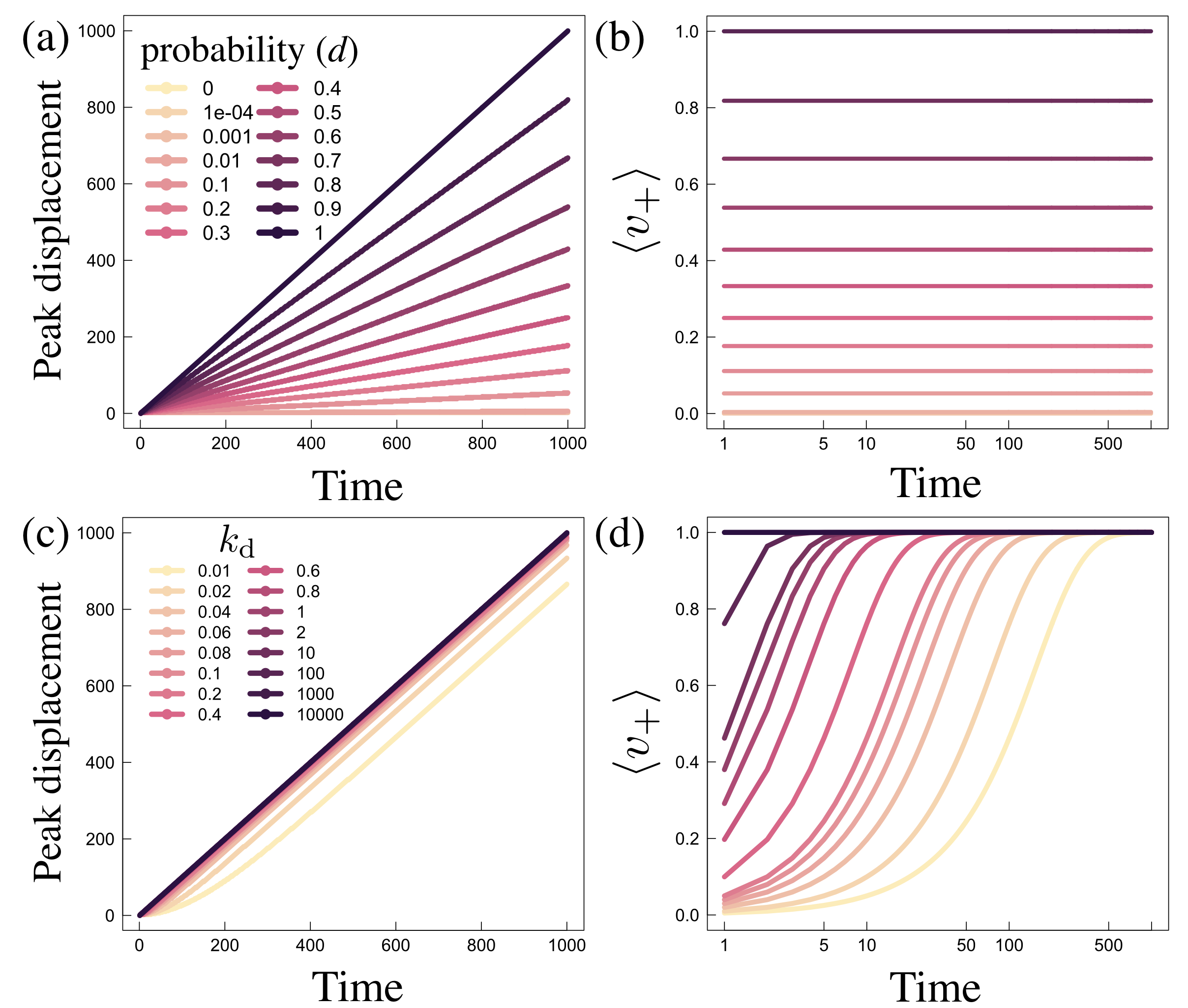
Figure 3: Ensemble-level analysis of positive peak displacement. (a) Positive peak displacement and (b) its velocity (13), as a function of time for constant detachment. (c) Positive peak displacement and (d) its velocity (14) as a function of time for exponential detachment.

Despite our system moving with equidistant jump lengths, with equal probability in either direction, and at constant time intervals, the detachment protocol alone is sufficient to push the anomalous diffusion exponent far into the superballistic regime for hundreds of time steps. Therefore, despite no individual particle experiencing acceleration, the selective bias of the detachment protocol produces an ensemble acceleration sufficiently strong to push the diffusion exponent far into the superballistic regime. To the best of our knowledge, this is a new mechanism for anomalous diffusion.

IV.2 Trajectory-resolved analysis

We have shown in an analytically tractable ensemble-level analysis that biased detachment is sufficient to tune the anomalous diffusion exponent far into the superballistic regime. Next, we explore the effects of the biased exponential detachment probability (3) in a trajectory-resolved analysis.

For each $k_{\rm d}$, we simulate $5\times 10^{4}$ independent trajectories. Figure 4a displays the proportion of trajectories still continuing at different times: as $k_{\rm d}$ increases, detachment happens more rapidly.

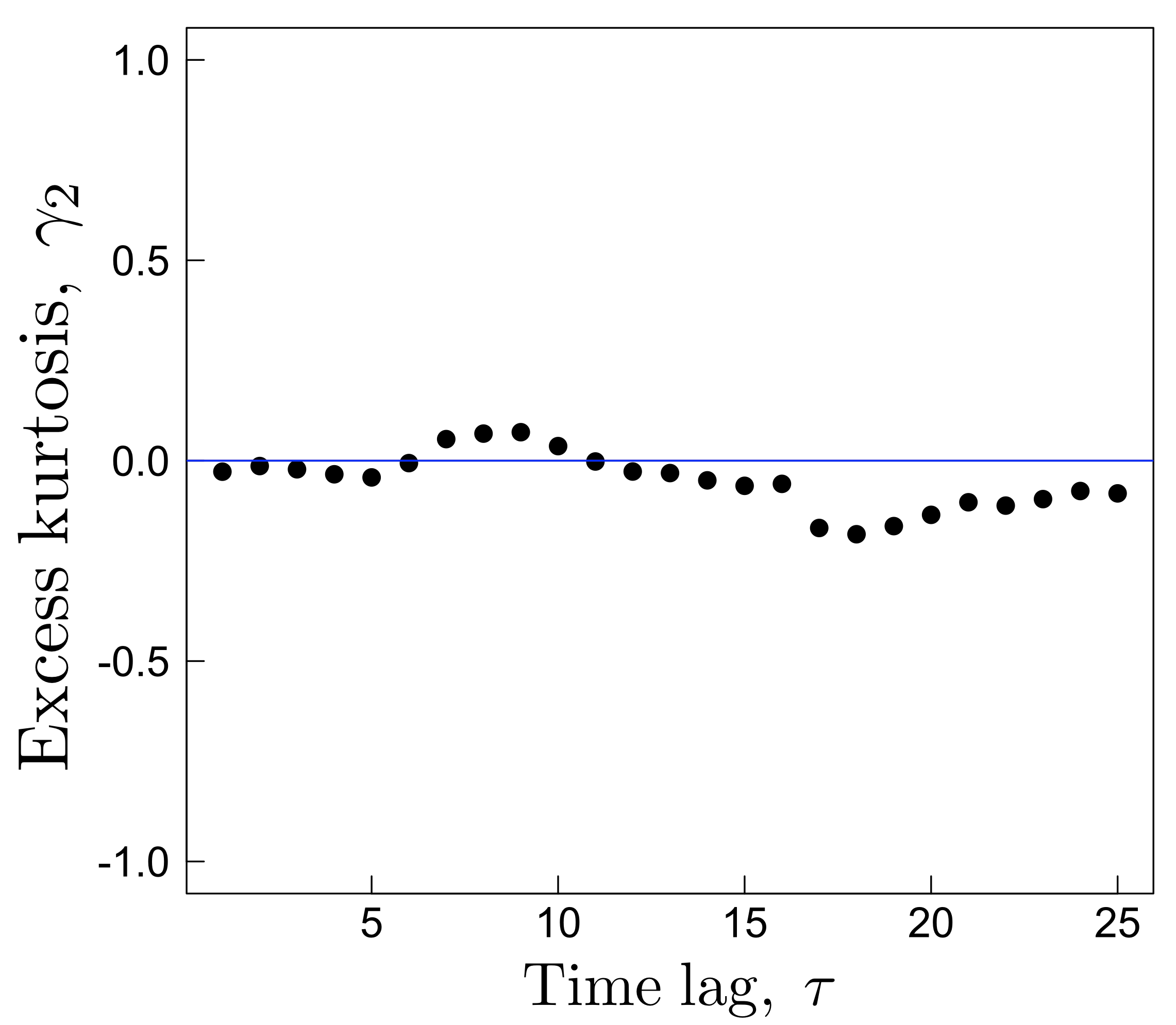
Figure 10: Excess kurtosis as a function of time lag for the trajectory-resolved model with $k_{\rm d}=0.005$.

We use the Gaussian parameter $\gamma_{2}$ (12) to determine if the displacement distribution conforms to a Gaussian, which is thought to be a requirement for conventionally diffusive systems Metzler and Klafter (2000). For all $k_{\rm d}$, the displacement distribution is well approximated by a Gaussian distribution. As an example, Figure 4b shows the displacement distribution for time lags $\tau=5$, 10, and 20 for $k_{\rm d}=0.005$. Figure 10 in Appendix E shows that $\gamma_{2}$ is close to 0, the Gaussian limit, for these and other time lags.

Figures 4c and 4d show the MSD_EA (9) and the MSD_ETA (11) for all $k_{\rm d}$. The MSD_EA produces higher $\alpha_{\rm GLS}$ for every $k_{\rm d}$, with a maximum $\alpha_{\rm GLS}=2.2$ for $k_{\rm d}=10$, compared to $1.8$ from the MSD_ETA with the same $k_{\rm d}$. Whereas the MSD_EA breaks through the ballistic threshold, the MSD_ETA remains in the superdiffusive (sub-ballistic) regime.

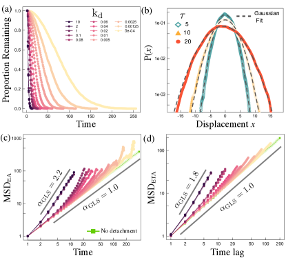
Figure 4: Trajectory-resolved analysis. (a) Proportion remaining as a function of time for various values of $k_{\rm d}$. (b) Example Gaussian fits to the displacement distribution for $k_{\rm d}=0.005$ and time lags $\tau=5,10,20$. (c) MSD_EA (9) as a function of time for each $k_{\rm d}$. (d) MSD_ETA (11) as a function of time for each $k_{\rm d}$.

For the trajectory-resolved analysis the highest $k_{\rm d}$ we explore is 10, where $\alpha_{\rm GLS}$ peaks at 2.2 and 1.8 for the MSD_EA and MSD_ETA, respectively (Fig. 4c,d). For the lowest $k_{\rm d}=5\times 10^{-4}$, $\alpha_{\rm GLS}$ barely increases above the no-detachment limit (Fig. 4c). This appears to be the opposite trend to that seen for the ensemble-level analysis (Fig. 2e); however, the limited statistics of remaining trajectories means that the trajectory-resolved analysis covers a shorter time range than does the ensemble-level approach.

To improve statistical significance, we simulate significantly more ($5\times 10^{5}$) trajectories for $k_{\rm d}=0.04$. Figure 5 shows trajectory-resolved MSD_EA (9) and MSD_ETA (11), alongside the ensemble-level MSD_EA. This comparison makes clear that all MSDs follow the same trend. It also highlights the statistical challenge of achieving superballistic behavior by biased detachment; however, even a small detachment bias ($k_{\rm d}=0.04$) produces significant superdiffusion.

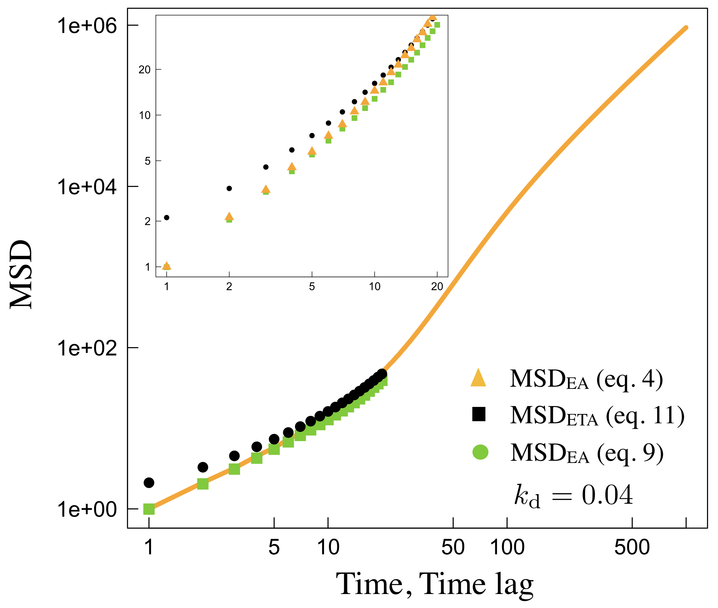
Figure 5: Trajectory-resolved MSD_ETA (11) (black squares) and MSD_EA (9) (green circles) compared with ensemble-level MSD_EA (4) (orange triangles and line), for $k_{\rm d}=0.04$ and 500,000 trajectories. Inset: all MSDs at short times or time lags.

IV.3 Analysis of longest-duration trajectories

Studies of molecular-motor transport commonly include in an MSD analysis only a subset of the recorded trajectories, often chosen because they remained associated to the track beyond a threshold duration Salman et al. (2002); Howse et al. (2007); Manley et al. (2008) or reached a certain distance Richard et al. (2019). Here we show that with biased detachment, selecting a longest-lived subset of the total ensemble biases the MSD analysis.

We simulate $2\times 10^{9}$ independent trajectories with $k_{\rm d}=0.05$, but only analyze subsets $M$ of these trajectories, selecting the $M_{1}=10^{2}$, $M_{2}=10^{4}$ and $M_{3}=10^{6}$ longest-duration trajectories for each subset (corresponding to proportions $5\times 10^{-8}$, $5\times 10^{-6}$, and $5\times 10^{-4}$, respectively). Figure 6a shows the detachment characteristics of these subsets: each $M$ sub-ensemble experiences a lag time before detachment begins. As the subset size decreases, detachment begins later. Figure 6b shows randomly selected trajectories from the longest-duration $M_{1}$ ensemble. Despite their clear stochasticity, they exhibit net motion away from the origin (as expected for these trajectories that avoided early origin-biased detachment).

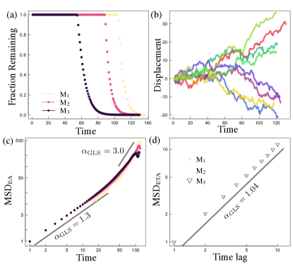
Figure 6: Longest-duration trajectory-resolved analysis. (a) Fraction remaining as a function of time for the $M$ longest-lived trajectories out of the total ensemble size of $2\times 10^{9}$. (b) Randomly selected trajectories from the longest-lived $M_{1}$ ensemble. (c) MSD_EA (9) and (d) MSD_ETA (11) as a function of time for all $M$ ensembles. All three ensembles give indistinguishable MSD_ETA.

Figure 6c displays MSD_EA as a function of time for all three $M$ ensembles. At early times (where no trajectories detach) the diffusion exponent $\alpha_{\rm GLS}=1.3$, exceeding conventional diffusion. After the onset of detachment, $\alpha_{\rm GLS}$ increases far into the superballistic regime and peaks at $3.0$, as measured by a generalized least squares fit of the $M_{1}$ ensemble over the time interval indicated by the black slanted line in Fig. 6c. Figure 6d shows MSD_ETA as a function of time, where—by contrast—$\alpha\approx 1$ for all sub-ensembles.

The longest-lived trajectories are those that have managed to escape the ‘detachment trap’ by successively moving away from the origin. That is, although the motion is random, from a sufficiently large ensemble there will be walkers that appear superdiffusive. It is therefore expected that the longest-lived ensembles exhibit superdiffusive characteristics even before the onset of detachment, as shown in Fig. 6c. There is a stark disparity between the MSD measures, with the MSD_EA strongly superdiffusive ($\alpha=1.3$, Fig. 6c) and the MSD_ETA only slightly superdiffusive ($\alpha=1.04\pm 0.01$, Fig. 6d). These results suggest that selecting a subset of trajectories based on processivity has the potential to strongly bias inferences about the system dynamics.

IV.4 Application to burnt-bridges ratchets

Some synthetic biomolecular systems, such as molecular spiders Pei et al. (2006); Lund et al. (2010), burnt-bridges ratchets Kovacic et al. (2015) and DNA nanomotors Yehl et al. (2015); Blanchard et al. (2019); Bazrafshan et al. (2020), remodel their tracks as they move and have been engineered to achieve directional motion at the molecular level. This remodeling turns a substrate site into a product site, and where there is a greater affinity to bind to substrate, motion is biased away from the product wake. Therefore, such systems have an increased probability of detachment from their tracks if they move backwards (into their product wake) Samii et al. (2010, 2011); Olah and Stefanovic (2013); Korosec et al. (2018).

To demonstrate that the anomalous $\alpha$ shown above is observed in more realistic systems with finite processivity, we examine simulated trajectories of a burnt-bridges ratchet (BBR), reported previously Korosec et al. (2018). Here, we examine an ensemble of 10,000 independent BBRs each moving on a quasi-1D track that is 4 lattice sites wide. Each BBR has 3 catalytic legs with a span of 8 lattice sites, which can each interact with substrate sites but not product sites. Figure 7 shows that the MSD_EA (9) and MSD_ETA (11) are quantitatively different. This is not surprising, because initial symmetry breaking leads to distinct short-time and long-time dynamics. In the long-time limit, both the MSD_EA (9) and MSD_ETA (11) produce superballistic $\alpha_{\rm GLS}$ (2.19 and 2.17, respectively). As no acceleration is imposed on the system, the breach above the ballistic threshold likely arises, as above, from the origin-directed detachment bias inherent to the BBR dynamics. We note that this apparent superballistic behavior is for a specific example of BBRs described in Korosec et al. (2018) and may not be a general result for all BBR systems.

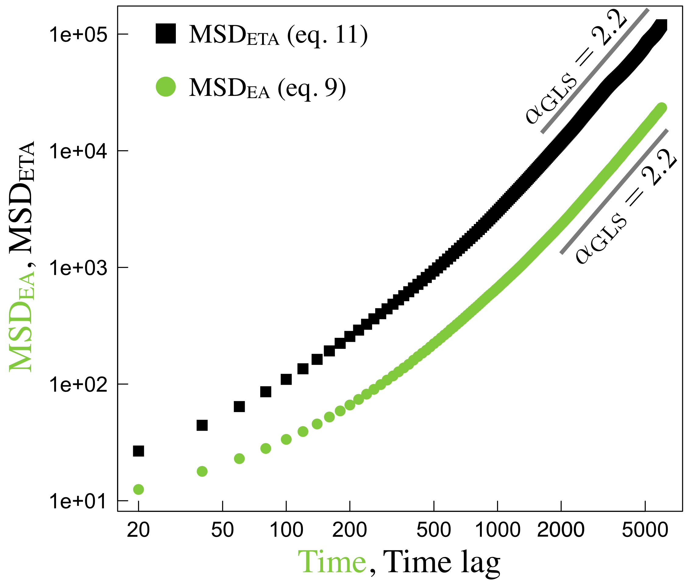
Figure 7: MSD_EA as a function of time (green) and MSD_ETA as a function of time lag (black) for burnt-bridges ratchets with finite processivity Korosec et al. (2018).

V Implications

V.1 Biological molecular motors

MSD analysis is often utilized in investigations of molecular motor dynamics. It has been applied to motors such as kinesin Inoue et al. (2001), dynein Ross et al. (2006) and myosin Brunstein et al. (2009). Of relevance to this work, all of these motors exhibit finite processivity: no molecular motor remains bound to its track forever. This finite processivity was the inspiration for the longest-lived analysis of Sec. IV.3: could duration-based selection of trajectories alter the conclusions drawn from MSD analysis? For example, when calculating the MSD_TA (10) from experimental data it is common to include only those motors that remained bound to the track for a certain time Salman et al. (2002); Howse et al. (2007); Manley et al. (2008), thereby ignoring those that detached. The selection of trajectories for MSD analysis is not always described, which makes it difficult for the interested reader to assess any bias that may manifest in the MSD. (We expect ensemble selection is not typically described in detail because the resulting potential bias in the MSD has not been raised before.) To our knowledge there are no experimental studies that examine how the MSD changes as a function of the duration of the trajectories chosen. Such sub-sampling would demonstrate the robustness of the conclusions drawn from the MSD, and could potentially provide mechanistic insight about detachment kinetics. For example, sub-sampling may indicate a directional detachment bias, as suggested by the work presented in this manuscript.

V.2 Random walks with finite processivity

Much attention has focused on understanding systems displaying anomalous diffusion. Anomalous diffusion is often correlated with non-Gaussian displacement distributions Joseph Phillies (2015); Wang et al. (2012). By contrast, here we demonstrate that a system with a Gaussian displacement distribution (Fig. 4b) can exhibit strongly anomalous diffusion. When simulating individual trajectories, our displacements are drawn from a Gaussian distribution. Anomalous diffusion is achieved by the consequences of the step direction: the walker faces an enhanced probability of detachment only if its step is towards the origin. Thus, the trajectories that tend towards the origin are filtered out as time progresses, thereby splitting the central mode into two symmetric modes about the origin (Fig. 2). However, the displacement distribution for the entire ensemble is Gaussian (Fig. 4b) because the stepping dynamics are inherently Gaussian, as in regular diffusion. The distinction giving rise to superdiffusion (and even, at times, superballistic characteristics) is the preferential truncation of trajectories that step towards the origin.

VI Conclusions

The MSD is commonly used to assess anomalous diffusion in microscopic systems. Here we assessed the effect of a biased detachment probability on the MSD of one-dimensional random walkers, employing both constant and exponential detachment probabilities. We found that the detachment rate controls the apparent dynamics of the system: more gradual detachment (smaller $k_{\rm d}$) delays the onset of superballistic behavior, but results in a larger and longer-lasting excursion into the superballistic regime (Fig. 2d). All of these biased-detachment systems eventually relax to the ballistic limit ($\alpha=2$). Fig. 5 shows a comparison between the trajectory and ensemble approaches where the superballistic behavior is most clearly seen in the (much longer-time) ensemble-level model. The limited statistics arising from detachment of trajectory-resolved systems means they cannot easily provide measures of long-time superballistic behaviors; however, the statistics are sufficient to demonstrate a strong superdiffusive bias.

The detachment bias confounds our ability to infer dynamical properties: the MSD suggests highly anomalous behavior, while the underlying dynamics we have imposed are Brownian. Therefore, for systems with trajectories of varying duration, a superdiffusive MSD should not on its own be taken to demonstrate directionality of a walker; such insight would require deconvolving the effects of processivity.

Researchers have cautioned about over-interpretation of the MSD for continuous-time random walks with power-law waiting-time distributions, where improper averaging can lead to false conclusions about transport properties Lubelski et al. (2008). We further caution the use of the MSD for systems with finite processivity, where detachment bias may lead to an overestimate of the anomalous diffusion exponent.

VII Acknowledgements

This work was funded by the Natural Sciences and Engineering Research Council of Canada (NSERC) through Discovery Grants to NRF and DAS and a Postgraduate Scholarship–Doctoral to CSK, and by a Tier-II Canada Research Chair to DAS. Computational resources were provided by Compute Canada.

Appendix A: Analytical expression for diffusion exponent $\alpha$

The ensemble-averaged mean-squared displacement is defined as

$$\left\langle[r(n)-r(0)]^{2}\right\rangle=\frac{1}{N}\sum_{i=1}^{N}[r_{i}(n)-r_{i}(0)]^{2}=D_{\rm g}n^{\alpha}.$$ (15)

Here, $n$ is an arbitrary point in time, $N$ is the size of the ensemble, $D_{\rm g}$ is the general diffusion coefficient and $\alpha$ is the anomalous diffusion exponent. We can also consider a point $n-b$ somewhat earlier in time:

$$\left\langle[r(n-b)-r(0)]^{2}\right\rangle=D_{\rm g}(n-b)^{\alpha}.$$ (16)

The ratio of (15) and (16) gives

$$\frac{\left\langle[r(n)-r(0)]^{2}\right\rangle}{\left\langle[r(n-b)-r(0)]^{2}\right\rangle}=\frac{n^{\alpha}}{(n-b)^{\alpha}},$$ (17)

$$\begin{split}\log_{n}\frac{\left\langle[r(n)-r(0)]^{2}\right\rangle}{\left\langle[r(n-b)-r(0)]^{2}\right\rangle}={}&\log_{n}\frac{n^{\alpha}}{(n-b)^{\alpha}}\end{split}$$ (18)

$$\begin{split}={}&\alpha\log_{n}n\\ &-\log_{n}[(n-b)^{\alpha}].\end{split}$$ (19)

Using the logarithmic identity

$$\log_{b}x=\frac{\log_{d}x}{\log_{d}b}$$ (20)

we then solve for $\alpha$,

$$\log_{n}\frac{\left\langle[r(n)-r(0)]^{2}\right\rangle}{\left\langle[r(n-b)-r(0)]^{2}\right\rangle}=\alpha\left(1-\frac{1}{\log_{n-b}n}\right),$$ (21)

$$\alpha^{n}_{n-b}=\left(1-\frac{1}{\log_{n-b}n}\right)^{-1}\log_{n}\frac{\left\langle[r(n)-r(0)]^{2}\right\rangle}{\left\langle[r(n-b)-r(0)]^{2}\right\rangle}\ .$$ (22)

The $\alpha^{n}_{n-b}$ notation denotes that $\alpha$ is estimated by two points, at times $n$ and $n-b$. Equation (22) is an expression for $\alpha$ derived from an arbitrary ensemble-averaged mean-squared displacement. In the work presented in this manuscript we restrict ourselves to one dimension and have a system for which $\left\langle x\right\rangle=0$. Equation (22) then reduces to

$$\alpha^{n}_{n-b}=\left(1-\frac{1}{\log_{n-b}n}\right)^{-1}\log_{n}\frac{\left\langle x^{2}(n)\right\rangle}{\left\langle x^{2}(n-b)\right\rangle}\ .$$ (23)

In this work we apply (23) with $b=2$ to analytical ensemble-level results, to estimate the anomalous diffusion exponent over a duration of 2 timesteps.

Appendix B: Comparing the dynamic functional to newly derived $\alpha_{n-b}^{n}$

To demonstrate the utility of $\alpha_{n-b}^{n}$ (6), we determine the anomalous diffusion coefficient for an example in which biased detachment is suddenly turned on after 100 timesteps. Figure 8a shows conventional diffusion for the first 100 timesteps, after which there is a sudden increase in the MSD_EA. Figure 8b compares $\alpha$ determined using (6) and (5). The derivative used to calculate $\alpha_{\psi}$ via (5) is a smoothing spline derivative with cross-validation Wahba (1983), while the expression (6) for $\alpha_{n-b}^{n}$ is exact.

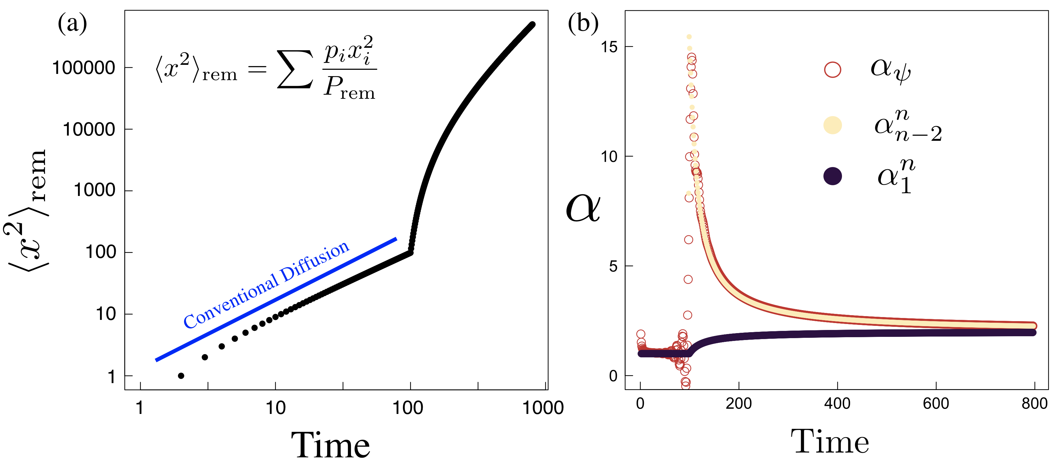
Figure 8: a) An example of a log-log MSD_EA-time trend from the analytical model where detachment is turned on at $t$=100. b) A comparison of $\alpha$ computed numerically by (5) and analytically by (6).

Appendix C: Analytical calculations for the discrete random walk with detachment

Table 2 provides sample analytical calculations from Table 1 of the ensemble-level MSD_EA (4) and the analytical anomalous diffusion exponent $\alpha^{n}_{n-2}$ derived in Appendix A, up to 4 timesteps. Here, $d$ is the probability of detachment (3), and $r\equiv 1-d$ represents the probability of remaining attached to the lattice for an individual step. $P_{\rm rem}$ is a normalization factor and represents the total probability of remaining attached to the lattice.

Table 2: $\left\langle x^{2}\right\rangle_{\rm rem}$ and $\alpha^{n}_{n-2}$ for the first 4 timesteps.

Timestep	$P_{\rm rem}$	$\sum p_{i}x_{i}^{2}$	$\left\langle x^{2}\right\rangle_{\rm rem}$	$\alpha^{n}_{n-2}$
0	1	0	0	/
1	1	1	1	/
2	$\frac{1}{2}(1+r)$	2	$\frac{4}{1+r}$	/
3	$\frac{1}{4}(1+3r)$	$\frac{3}{4}(3+r)$	$\frac{9+3r}{1+3r}$	$\log_{3}\frac{9+3r}{1+3r}$
4	$\frac{1}{8}$ + $\frac{1}{2}r$ + $\frac{3}{8}r^{2}$	$2(1+r)$	$\frac{16}{1+3r}$	$2\log_{4}\frac{4(r+1)}{3r+1}$

Appendix D: Derivation of $\left\langle v_{+}\right\rangle$ for the ensemble-level model

Here we derive a general expression for the ensemble-level $\left\langle v_{+}\right\rangle$, the mean velocity conditioned on the walker being at positive displacement. We consider a discrete system in one dimension that can take steps to the left or right with step size $|\Delta x|=1$ and $\Delta t=1$. The probability of stepping left or right is equal. Let $d_{\rm l}(t)$ and $d_{\rm r}(t)$ represent the probability of detaching from the lattice for steps taken to the left and right, respectively. We then write the normalized probability at time $t$ of taking a step to the left and remaining attached as

$$P(\Delta x_{\rm left})=\frac{1-d_{\rm l}(t)}{2-d_{\rm l}(t)-d_{\rm r}(t)},$$ (24)

and the normalized probability of taking a step to the right and remaining attached as

$$P(\Delta x_{\rm right})=\frac{1-d_{\rm r}(t)}{2-d_{\rm l}(t)-d_{\rm r}(t)}.$$ (25)

Thus, the average displacement after one timestep is $\left\langle\delta x\right\rangle=[P(\Delta x_{\rm right})-P(\Delta x_{\rm left})]\Delta x$. Then

$$\left\langle v_{+}\right\rangle=\frac{\left\langle\delta x\right\rangle}{\Delta t}=\frac{d_{\rm l}(t)-d_{\rm r}(t)}{2-d_{\rm l}(t)-d_{\rm r}(t)}\frac{\Delta x}{\Delta t}\ .$$ (26)

The effects of detachment on the mean ensemble acceleration $\left\langle a_{+}\right\rangle=\frac{\mathrm{d}}{\mathrm{d}t}\left\langle v_{+}\right\rangle$ can then be determined, as can the conditional mean displacement: $\left\langle x_{+}\right\rangle=\int\mathrm{d}t\left\langle v_{+}\right\rangle$.

In this work we consider exponential detachment for particles moving towards the origin: $d_{\rm r}(t)=0$ and $d_{\rm l}(t)=d(t)=1-e^{-k_{\rm d}t}$. We then have

$${\left\langle v_{+}\right\rangle}_{\rm exp}=\frac{1-e^{k_{\rm d}t}}{1+e^{-k_{\rm d}t}}.$$ (27)

We also consider the case where detachment towards the origin is constant with time, $d_{\rm r}(t)=0$ and $d_{\rm l}(t)=d$, giving

$${\left\langle v_{+}\right\rangle}_{\rm const}=\frac{d}{2-d}.$$ (28)

To demonstrate agreement of this approach with our numerical data, we compare for the exponential case the positive peak displacement obtained from the ensemble-level simulations with the analytical conditional mean

$${\left\langle x_{+}\right\rangle}_{\rm exp}={} \int\mathrm{d}t\frac{1-e^{k_{\rm d}t}}{1+e^{-k_{\rm d}t}}$$ (29)

$$={} \frac{2\log({e^{k_{\rm d}t}+1})}{k_{\rm d}}-t+C,$$ (30)

where $C$ is an integration constant. We set the integration constant to $C=-\frac{2\log 2}{k_{\rm d}}$ such that $\langle x_{+}\rangle_{\rm exp}(t=0)=0$. We find this analytical expression for $\langle x_{+}\rangle_{\rm exp}$ to agree with the ensemble-level results for exponential detachment (Fig. 9).

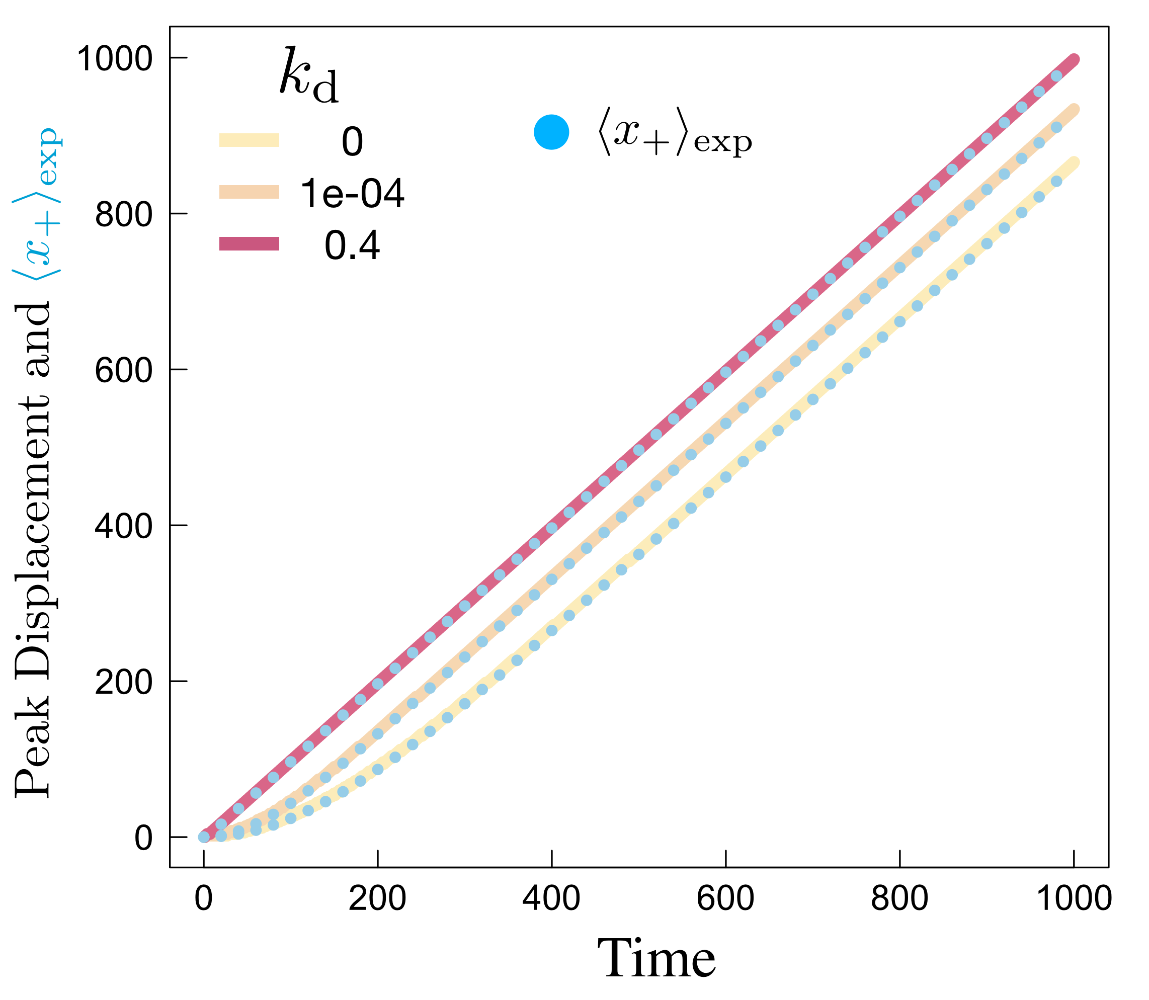
Figure 9: Conditional mean $\langle x_{+}\rangle_{\rm exp}$ (29) (blue dots) from theory agrees with ensemble-level positive peak displacement (curves) from Fig. 3c.

Appendix E: Further Kurtosis Analysis of trajectory-resolved model

Here we plot the excess kurtosis as a function of time lag for $k_{\rm d}=0.005$ of the trajectory-resolved simulations. We find that at all time lags the excess kurtosis is close to the Gaussian limit of 0.

References

- Einstein (1956) A. Einstein, Courier Corporation (1956).
- Metzler and Klafter (2000) R. Metzler and J. Klafter, Phys. Rep. 339, 1 (2000).
- Richardson (1926) L. F. Richardson, Proc. R. Soc. London 110, 709 (1926).
- Havlin and Ben-Avraham (2002) S. Havlin and D. Ben-Avraham, Adv. Phys. 51, 187 (2002).
- Metzler et al. (2014) R. Metzler, J. H. Jeon, A. G. Cherstvy, and E. Barkai, Phys. Chem. Chem. Phys. 16, 24128 (2014).
- Bao and Zhuo (2003) J. D. Bao and Y. Z. Zhuo, Phys. Rev. Lett. 91, 138104 (2003).
- Feinerman et al. (2018) O. Feinerman, I. Pinkoviezky, A. Gelblum, E. Fonio, and N. S. Gov, Nat. Phys. 14, 683 (2018).
- Rank et al. (2013) M. Rank, L. Reese, and E. Frey, Phys. Rev. E 87, 032706 (2013).
- ben-Avraham et al. (1992) D. ben-Avraham, F. Leyvraz, and S. Redner, Phys. Rev. A 45, 2315 (1992).
- Tilles et al. (2017) P. F. Tilles, S. V. Petrovskii, and P. L. Natti, Sci. Rep. 7, 1 (2017).
- Li et al. (2010) T. Li, S. Kheifets, D. Medellin, and M. G. Raizen, Science 328, 1673 (2010).
- Duplat et al. (2013) J. Duplat, S. Kheifets, T. Li, M. G. Raizen, and E. Villermaux, Phys. Rev. E 87, 020105(R) (2013).
- Cherstvy and Metzler (2016) A. G. Cherstvy and R. Metzler, Phys. Chem. Chem. Phys. 18, 23840 (2016).
- Le Vot et al. (2017) F. Le Vot, E. Abad, and S. B. Yuste, Phys. Rev. E 96, 032117 (2017).
- Salman et al. (2002) H. Salman, Y. Gil, R. Granek, and M. Elbaum, Chem. Phys. 284, 389 (2002).
- Howse et al. (2007) J. R. Howse, R. A. L. Jones, A. J. Ryan, T. Gough, R. Vafabakhsh, and R. Golestanian, Phys. Rev. Lett. 99, 048102 (2007).
- Manley et al. (2008) S. Manley, J. M. Gillette, G. H. Patterson, H. Shroff, H. F. Hess, E. Betzig, and J. Lippincott-Schwartz, Nat. Methods 5, 155 (2008).
- Kepten et al. (2013) E. Kepten, I. Bronshtein, and Y. Garini, Phys. Rev. E 87, 052713 (2013).
- Ghosh et al. (2016) S. K. Ghosh, A. G. Cherstvy, D. S. Grebenkov, and R. Metzler, New J. Phys. 18, 013027 (2016).
- Karmakar et al. (2016) S. Karmakar, C. Dasgupta, and S. Sastry, Phys. Rev. Lett. 116, 085701 (2016).
- Martin et al. (2002) D. S. Martin, M. B. Forstner, and J. A. Käs, Biophys. J. 83, 2109 (2002).
- van Hove (1954) L. van Hove, Phys. Rev. 95, 249 (1954).
- Akcasu et al. (1970) A. Z. Akcasu, N. Corngold, and J. J. Duderstadt, Phys. Fluids 13, 2213 (1970).
- Cherstvy et al. (2019) A. G. Cherstvy, S. Thapa, C. E. Wagner, and R. Metzler, Soft Matter 15, 2526 (2019).
- Bel and Barkai (2005) G. Bel and E. Barkai, Phys. Rev. Lett. 94, 240602 (2005).
- Orsini and Greenland (2009) N. B. R. Orsini and S. Greenland, Stata J 6, 40 (2009).
- Rahman (1964) A. Rahman, Phys. Rev. 136, A405 (1964).
- Kob and Andersen (1995) W. Kob and H. C. Andersen, Phys. Rev. E 51, 4626 (1995).
- Richard et al. (2019) M. Richard, C. Blanch-Mercader, H. Ennomani, W. Cao, and M. Enrique, PNAS 116, 14835 (2019).
- Pei et al. (2006) R. Pei, S. K. Taylor, D. Stefanovic, S. Rudchenko, T. E. Mitchell, and M. N. Stojanovic, J. Am. Chem. Soc. 128, 12693 (2006).
- Lund et al. (2010) K. Lund, A. J. Manzo, N. Dabby, N. Michelotti, A. Johnson-Buck, J. Nangreave, S. Taylor, R. Pei, M. N. Stojanovic, N. G. Walter, E. Winfree, and H. Yan, Nature 465, 206 (2010).
- Kovacic et al. (2015) S. Kovacic, L. Samii, P. M. Curmi, H. Linke, M. J. Zuckermann, and N. R. Forde, IEEE Trans. Nanobioscience 14, 305 (2015).
- Yehl et al. (2015) K. Yehl, A. Mugler, S. Vivek, Y. Liu, Y. Zhang, M. Fan, E. R. Weeks, and K. Salaita, Nat. Nano. 11, 184 (2015).
- Blanchard et al. (2019) A. T. Blanchard, A. S. Bazrafshan, J. Yi, J. T. Eisman, K. M. Yehl, T. Bian, A. Mugler, and K. Salaita, Nano Lett. 19, 6977 (2019).
- Bazrafshan et al. (2020) A. Bazrafshan, T. Meyer A, H. Su, J. Brockman M, A. Blanchard T, S. Pirane, Y. Duan, Y. Ke, and K. Salaita, Angew. Chem. Int. Ed. (2020).
- Samii et al. (2010) L. Samii, H. Linke, M. J. Zuckermann, and N. R. Forde, Phys Rev E 81, 021106 (2010).
- Samii et al. (2011) L. Samii, G. A. Blab, E. H. C. Bromley, H. Linke, P. M. G. Curmi, M. J. Zuckermann, and N. R. Forde, Phys Rev E 84, 031111 (2011).
- Olah and Stefanovic (2013) M. J. Olah and D. Stefanovic, Phys. Rev. E 87, 062713 (2013).
- Korosec et al. (2018) C. S. Korosec, M. J. Zuckermann, and N. R. Forde, Phys. Rev. E 98, 032114 (2018).
- Inoue et al. (2001) Y. Inoue, A. H. Iwane, T. Miyai, E. Muto, and T. Yanagida, Biophys. J. 81, 2838 (2001).
- Ross et al. (2006) J. L. Ross, K. Wallace, H. Shuman, Y. E. Goldman, and E. L. F. Holzbaur, Nat. Cell Biol. 8, 562 (2006).
- Brunstein et al. (2009) M. Brunstein, L. Bruno, M. Desposito, and V. Levi, Biophys. J. 97, 1548 (2009).
- Joseph Phillies (2015) G. D. Joseph Phillies, Soft Matter 11, 580 (2015).
- Wang et al. (2012) B. Wang, J. Kuo, S. C. Bae, and S. Granick, Nat. Mater. 11, 481 (2012).
- Lubelski et al. (2008) A. Lubelski, I. M. Sokolov, and J. Klafter, Phys. Rev. Lett. 100, 250602 (2008).
- Wahba (1983) G. Wahba, J.R. Stat. Soc. B 45, 133 (1983).