Toward the Detection of Relativistic Image Doubling in Water Cherenkov Detectors

Abstract

When a gamma or cosmic ray strikes the top of Earth’s atmosphere, a shower of secondary particles moves toward the surface. Some of these secondary particles are charged muons that subsequently enter Water Cherenkov Detectors (WCDs) on the ground. Many of these muons, traveling near the speed of light in vacuum, are moving faster than the speed of light in water and so trigger isotropic Cherenkov radiation in the WCDs. Inside many WCDs are photomultiplier tubes (PMTs) that detect this Cherenkov radiation. When the radial component of the speed of a muon toward a PMT drops from superluminal to subluminal, the PMT will record Cherenkov light from a little-known optical phenomenon called Relativistic Image Doubling (RID). Were the RID-detecting PMTs replaced by high resolution video recorders, they would see two Cherenkov images of the muon suddenly appear inside the tank, with one image moving with a velocity component toward the recorders, the other away. Even without a video, the RID phenomenon will cause different PMTs to record markedly different light curves for the same muon. In this paper, we present a study hoping to inspire the explicit detection and reporting of RID effects in WCDs. We consider three example cases of muon RIDs in High-Altitude Water Cherenkov (HAWC)-like systems: vertical, horizontal and oblique. Monte Carlo simulations show that RID effects in HAWC-like systems are not rare – they occur for over 85 percent of all muon tracks.

1 Introduction

Air showers of fundamental particles result when a single high energy particle such as a gamma-ray strikes the top of the Earth’s atmosphere (Rossi, 1933). A common type of secondary shower particle is the charged muon which decays in 2.2 microseconds in its own inertial frame (Tanabashi et al., 2018), but in the frame of the Earth, its relativistic speed can cause it to last much longer. Long time delays allow relativistic muons to reach the surface before decaying.

At the surface, secondary muons may enter vats of water designed to detect them. The key to detection is the Cherenkov radiation (Čerenkov, 1937) that they cause in the water tanks, which is created because the speed of the charged muon is much greater than the speed of light in water.

Objects moving faster than light in a given medium may create images in non-classical ways. One recently studied example is Relativistic Image Doubling (RID) (Cavaliere et al., 1971; Nemiroff, 2015, 2018, 2019). With RID, objects moving superluminally in a medium (faster than the medium speed of light) can appear twice simultaneously to an observer. The RID illusion starts when the moving object’s speed toward this observer drops from superluminal to subluminal. At that time, two bright images of the objects suddenly appear and diverge. RID effects have recently been found in the lab (Clerici et al., 2016) and have been hypothesized to help explain light curves in gamma-ray bursts (Hakkila & Nemiroff, 2019). Most recently, it has been suggested that RID effects occur and can be commonly found in images of air showers by Imaging Atmospheric Cherenkov Telescopes (Nemiroff & Kaushal, 2020).

In this work, it will be shown that RID effects not only exist but are common for muon tracks in ground-based Water Cherenkov Detectors (WCDs). WCDs exist in many cosmic gamma-ray detectors today, including those deployed by Auger (Aab et al., 2015), HAWC (BenZvi, 2015), Kamiokande (Arisaka et al., 1984), and IceCube (Aartsen et al., 2017).

The paper is structured as follows. In Section 2 the conceptual basis for RIDs are reviewed in relation to how they might affect WCDs. Also we develop the mathematical framework behind the concepts, assuming the muon takes an arbitrary track in the WCD, and the detector is located at an arbitrary position on the WCD floor. In Section 3 we calculate what results would be expected from three different types of detectors: a video detector that records both the brightness of the muon track and its angular position with time, a digital camera that records the brightness as a function of angular position but not time, and a PMT that records brightness as a function of time but not angular position. Also, we show simulation results for an example WCD tank that is similar to the tanks in the High-Altitude Water Cherenkov (HAWC) observatory. In Section 4 it is shown how prevalent RIDs are in WCDs like HAWC, and how RID resolution might help decode the muon track. In Section 5 we discuss various aspects of RID in regard to its applications and future developments. Finally some of the codes used for the simulations are shown in Appendix.

2 RID: Concepts and Mathematics

Following Nemiroff & Kaushal (2020), several RID concepts are found to be relevant here. Consider a cosmic ray muon travelling with a speed $v>c_{w}$, where $c_{w}$ is the speed of light in water, and entering the top of a Water Cherenkov Detector (WCD) tank filled up to height $H$ and leaving the tank through the bottom. The speed $v$ of the muon is considered here to be constant during its entire track across the WCD. The muon enters the WCD at time $t=0$ and causes the emission of isotropic Cherenkov light in its immediate wake. Although not a direct image of the muon, this light will be referred to as a “Cherenkov image”.

The light is assumed to be seen here by a video detector that tracks both angular position and brightness in time. The detector, on the floor of the WCD, is assumed to be located at a distance $L$ from the point where the muon enters the WCD and at distance $M$ from the point where it exits the WCD. The path length traveled by the muon inside the tank is given by $P$. The height of the muon from the tank bottom at any time $t$ during its course in the tank is given by $z$. This is shown in Figure 1.

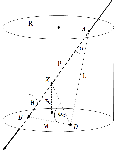
Figure 1: A muon entering the top of the WCD tank through $A$ and leaving the bottom through $B$. The path length of the muon inside the tank is given by $P$ while the distances of the detector $D$ from $A$ and $B$ are given by $L$ and $M$ respectively. $\alpha$ is the angle between the muon track and the detector through the entry point $A$.

Because of the superluminal speed (meaning $v>c_{w}$) of the muon, some muon tracks will appear to have non-classical attributes. Specifically, some muon tracks will be seen by the video detector to undergo relativistic image doubling (RID).

The velocity of the muon at any point in its trajectory can be considered to have two components relative to each detector – one radially toward (or away) from the detector ($v_{r}$), and one perpendicular to the line connecting the detector to the muon. If the detector is nearly in the path of the incoming muon, then $v_{r}>c$. Conversely, when the muon is closest to the detector, $v_{r}=0$. For this incoming muon, there will be a location in its track where $v_{r}$ drops from superluminal to subluminal at which the detector will see an RID. This is equivalent to that detector passing from outside to inside the Cherenkov cone of the muon. The video will record the muon’s Cherenkov images suddenly appearing at the location of the RID, typically away from the top or any edge of the WCD. The muon, as shown by its Cherenkov images, will then appear on the video to be at two places simultaneously, with one image moving along the original muon track, while a second image moving backwards along the entry track of the muon.

For some detector locations, the muon’s radial speed toward the detector is always subluminal, even though the total speed of the muon is always superluminal. These cases are the most classical, as the detector observes the muon move from the entry point in the tank, downward. In this case, no RID would be recorded by the video detector.

Let’s now concentrate on detectors which do see RID events. From the point of view of these detectors, muons will first traverse a region starting from their point of entry into the WCD and extending down to $z_{C}$ where $v_{r}=c_{w}$. In this region, the speed of the muon toward the detector $(v_{r})$ is faster than the speed of the Cherenkov radiation it causes. When eventually seen by the detector, this part of the muon track will be seen time-backwards, meaning that Cherenkov radiation emitted increasingly earlier along the track will reach the detector at increasingly later times. This part of the track will appear to go up from $z_{C}$. After the muon has descended down past $z_{C}$ however, the radial component of its speed will be slower than its Cherenkov light and so this part of the muon track will appear normally: time forwards and headed down. Thus the muon is first seen by the detector at height $z_{C}$ and not at the point of its entry in the tank.

The total time from when the muon enters the tank to when the detector records Cherenkov radiation from the muon’s trail can be broken up into two times, the time $t_{muon}$ taken by the muon to descend to a height $z$, and the time $t_{radiation}$ taken by the Cherenkov light to travel from $z$ to the detector. This combined time is denoted by $t_{total}$.

The critical height $z_{C}$ where the muon is first seen by the detector occurs at time $t_{min}$, when $t_{total}$ is a minimum. This can be found by solving $dt_{total}/dz=0$ for $z$. For a muon entering the tank from the top and leaving through the bottom, $z_{C}$ is given by

$${z_{C}=H-\Big{(}L\cos\alpha-\frac{c_{w}L\sin\alpha}{\sqrt{v^{2}-c_{w}^{2}}}\Big{)}\cos\theta,}$$ (1)

where $\theta$ is the angle the muon track makes with the vertical and $\alpha$ is the angle between the detector and the muon track through point $A$. The angular location, $\phi_{C}$, where the muon is first seen by the detector, is the angle between the line joining the detector $D$ with the location $X$ of critical height $z_{C}$ on the muon path (i.e. $DX$) and the line joining the detector with the exit point of muon at the WCD floor (i.e. $BD$). The distance between the detector $D$ and the location of first RID on the muon track $X$ is given by

$$\begin{split}DX&=\sqrt{AD^{2}+AX^{2}-2AX\cdot AD\cos\alpha}\\ &=\sqrt{L^{2}+\Big{(}P-\frac{z_{C}}{\cos\theta}\Big{)}^{2}-2L\cos\alpha\Big{(}P-\frac{z_{c}}{\cos\theta}\Big{)}}.\end{split}$$ (2)

Therefore,

$$\begin{split}\phi_{C}&=\arccos{\Big{(}\frac{BD^{2}+DX^{2}-BX^{2}}{2\cdot BD\cdot DX}\Big{)}}\\ &=\arccos{\Bigg{(}\frac{\left(P^{2}+L^{2}+M^{2}\right)\cos\theta+2L\cos\alpha(z_{C}-P\cos\theta)-2Pz_{C}}{2M\cos\theta\sqrt{L^{2}-2L\cos\alpha\left(P-\frac{z_{C}}{\cos\theta}\right)+\left(P-\frac{z_{C}}{\cos\theta}\right)^{2}}}\Bigg{)}}.\end{split}$$ (3)

Note that an angle $\phi_{C}=0^{\circ}$ corresponds to the line joining the detector and the exit point $B$. This is shown by the line segment $BD$ in Figure 1.

Near $z_{C}$, the muon’s speed toward the detector almost equals the speed of its liberated Cherenkov light. Therefore a relatively large amount of this light arrives at the detector “bunched up” – over a very short period of time (Nemiroff & Kaushal, 2020). It can then be said that at height $z_{C}$, the detector is on the “Cherenkov Cone”. Note that since Cherenkov light is emitted uniformly and isotropically along the muon’s trajectory in the frame of water, the Cherenkov Cone is a detector-dependent phenomenon.

After $t_{min}$, two images of the muon’s Cherenkov light are observed simultaneously by the detector at heights $z_{\pm}$ from the bottom of the tank, where $z_{+}$ and $z_{-}$ are always above and below $z_{C}$ respectively,

$${z_{\pm}=H-\Bigg{(}\frac{c_{w}^{2}t_{total}v-Lv^{2}\cos\alpha\pm\sqrt{v^{2}\left(c_{w}^{2}\left(L^{2}+t_{total}^{2}v^{2}\right)-2c_{w}^{2}Lt_{total}v\cos\alpha+L^{2}v^{2}\cos^{2}\alpha-L^{2}v^{2}\right)}}{c_{w}^{2}-v^{2}}\Bigg{)}\cos\theta.}$$ (4)

The angular locations of the two images as seen from the detector are given by

$${\phi_{\pm}=\arccos{\Bigg{(}\frac{\left(P^{2}+L^{2}+M^{2}\right)\cos\theta+2L\cos\alpha(z_{\pm}-P\cos\theta)-2Pz_{\pm}}{2M\cos\theta\sqrt{L^{2}-2L\cos\alpha\left(P-\frac{z_{\pm}}{\cos\theta}\right)+\left(P-\frac{z_{\pm}}{\cos\theta}\right)^{2}}}\Bigg{)}}.}$$ (5)

Once the height and time of each image of the pair is known, their velocities can be calculated by taking $v_{\pm}=dz_{\pm}/dt_{total}$. The apparent angular speeds ${\omega}_{\pm}$ of these images can be computed by dividing the transverse components of their speeds by their distances from the detector. The apparent brightness of an image is computed by integrating the instantaneous brightness of the track visible to the detector over a uniform time interval. However, since relatively long path lengths are seen over a uniform time interval when $v_{r}\sim c_{w}$, the apparent brightness $b$ of each image is proportional to its angular speed. At the extreme, when $v_{r}=c_{w}$, the apparent angular speed diverges and the length of the path visible to the detector will formally diverge even over an arbitrarily small time interval. In a separate effect, an image brightness falls by the square of its distance to the detector. Together, these effects yield image brightness of

$${b_{\pm}\propto{{{\omega_{\pm}}}\over{L^{2}+z_{\pm}^{2}}}}$$ (6)

Although it is cumbersome to expand this equation analytically because of the complexity of Eq. 4, it is straightforward to use this equation numerically. Formally, the brightness of the shower as recorded by the detector mathematically diverges, when the shower appears at “criticality” when $v_{r}=c_{w}$ at $z_{\pm}=z_{C}$. This divergence is mitigated in practice, however, by the muon’s track being of finite angular size.

3 Cases

Three example cases are examined here. The WCD tank is assumed to be similar to that used by HAWC. This tank is a cylinder with radius $R=3.65$ meters and height $5$ metres filled with water up to height $H=4.5$ meters (Sandoval, 2013). Four PMTs are assumed to be on the floor of the tank with one in the center and three uniformly spread in a Y-pattern, each at a distance of 1.85 meters from the central PMT (Hüentemeyer, private communication). A three-dimensional view of the system is depicted in Figure 2. Inside this WCD, three types of detectors will be considered. The first is a video detector with the ability to resolve Cherenkov images in both time and angle. The second is a static camera with angular but not time resolving abilities and the third is a PMT which can resolve brightness with time but not with angle.

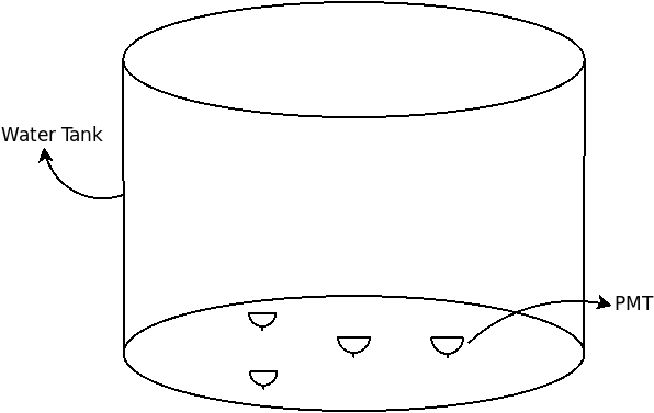
Figure 2: A Three-Dimensional representation of a HAWC-like Water Cherenkov Detection (WCD) tank. The placement of the PMTs on the tank floor is also shown. A bird’s eye view of this tank is shown in Figure 6 along with a track for a muon entering horizontally.

3.1 Vertical Incidence

The first case considered is particularly simple and formulated to calibrate intuition. In this case, the muon enters the WCD vertically moving straight down and directly striking the central detector. The detectors are all considered to be video detectors, at first. The only Cherenkov image visible to the central detector in this scenario is the one moving upwards, which, counter-intuitively, is in the opposite direction of the actual downward motion of the muon! The three surrounding detectors will see the same Cherenkov image motions as they are all at the same distance from the muon track as well as the central detector, and symmetrically oriented. The first event these detectors will see is the pair creation event or RID. After that, each detector will record the two Cherenkov images of the muon track moving in geometrically opposite directions along the original track. The video detector in this case will see the development of Cherenkov images along the muon track with time. Data extracted from the resulting video would show the angular position of the Cherenkov images versus time as shown in Figure 3.

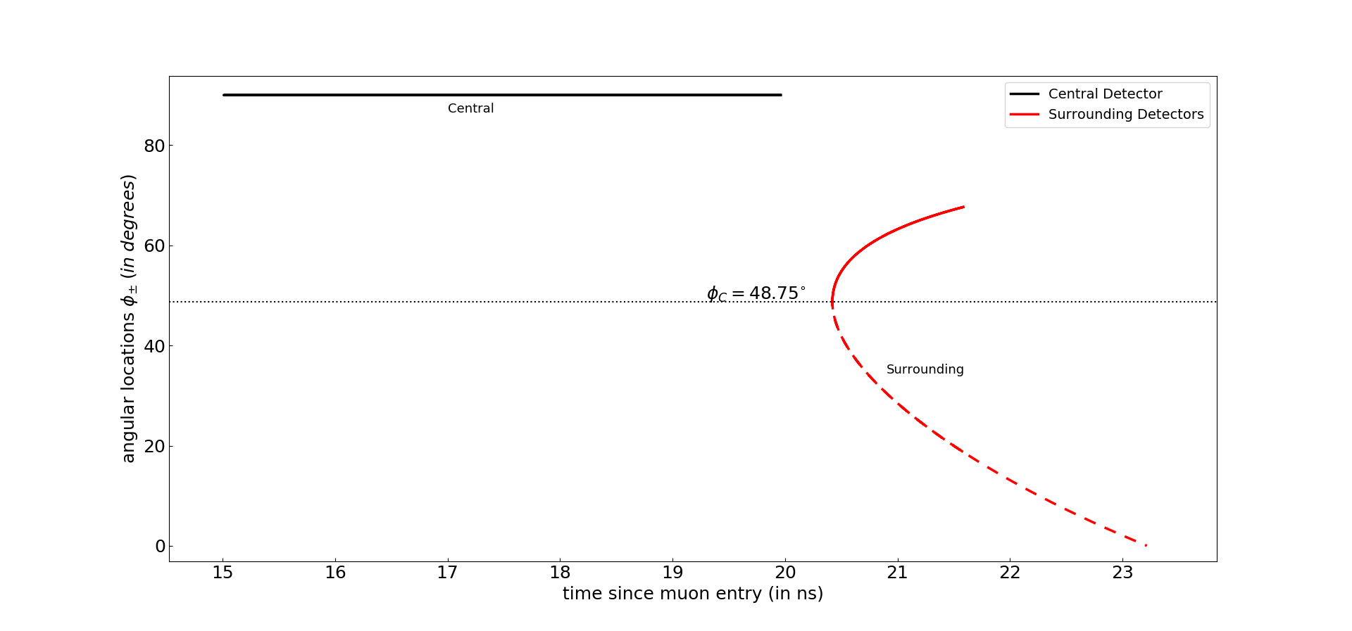
Figure 3: A plot of angular location of Cherenkov images versus time for a muon entering the WCD straight down and striking the central detector at the bottom of the tank. A solid curve represents the Cherenkov image moving upwards while a dashed curve means that the image is moving downwards. The three surrounding detectors are at 1.85 meters from the central one and thus the red curve shown is the same for all three detectors. $\phi_{C}$ denotes the angular location for the first RID and corresponds to the critical height $z_{C}$.

Simpler than a video, a static digital camera image will record a line that encodes the variation of brightness of Cherenkov images with their corresponding angular locations. This can be seen from the inspection of Figure 4.

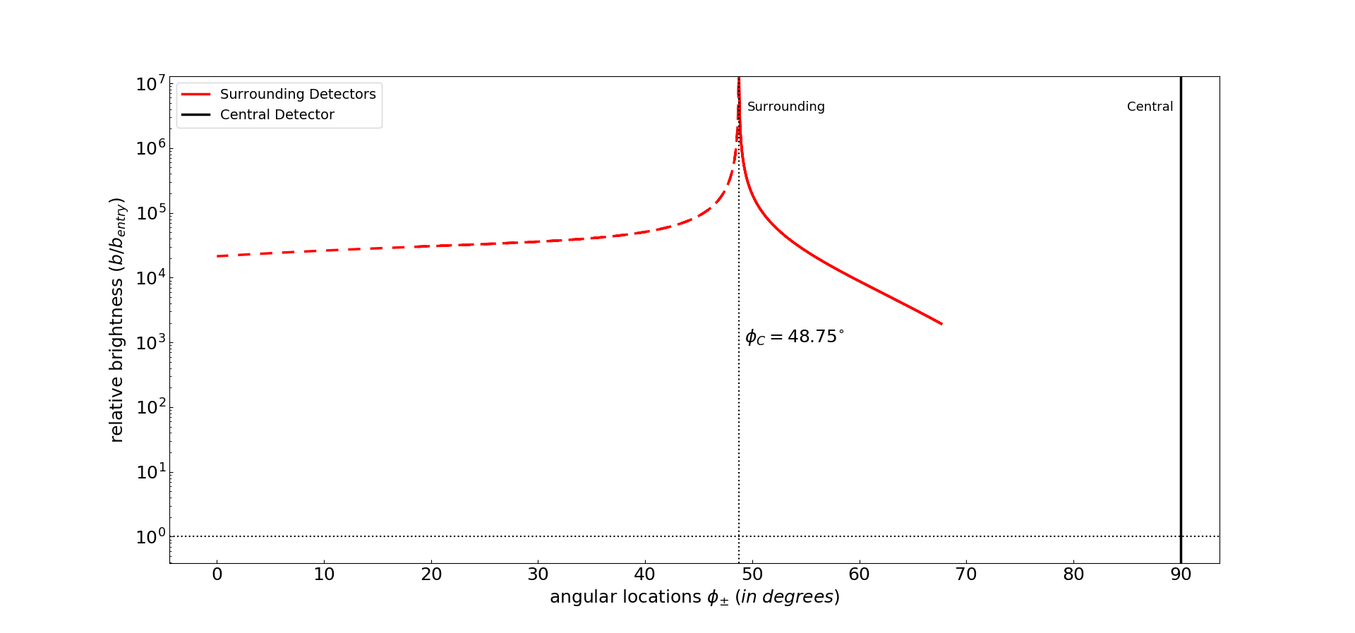
Figure 4: A graph of relative image brightness versus the angular locations of the Cherenkov images of a muon moving straight down and striking the central detector. The central detector always sees a Cherenkov image directly above it at $\phi=90$ degrees.

The third possible detector type, the time-sensitive PMT, will record only a light curve – a plot of image brightness versus time. The light curve of the vertically descending muon (which results in a single vertically ascending Cherenkov image) is shown in Figure 5.

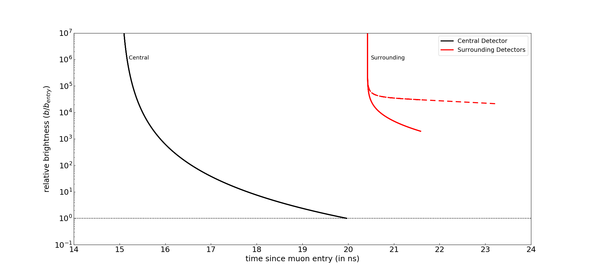
Figure 5: A plot of relative brightness versus time for the Cherenkov images observed in the case of a muon moving straight down and then striking the central detector. After observing the first RID at 20.42 ns, the three surrounding video detectors will see two images of the muon track with time, with one fainter than the other. The image going up towards the entry point will not be observable after 21.58 ns but the one going down will continue to be seen till 23.22 ns. Because the two images usually differ so much in brightness, a PMT detector will effectively measure only the light curve of the brighter of the two images.

3.2 Horizontal Incidence

This case considers the muon travelling horizontally through the water entering the tank at point $A(x_{1},\sqrt{R^{2}-x^{2}_{1}},h)$ and leaving through $B(x_{2},\sqrt{R^{2}-x^{2}_{2}},h)$, where the muon incidence height $h$ can be anywhere between $0$ and $H$. In correspondence with critical height $z_{C}$ for a downward moving muon, a critical distance $x_{C}$ from entry point $A$ exists where, if $x_{C}<AB$, where $AB$ is the distance between $A$ and $B$, the detector will be exposed to a pair event at $x_{C}$. The location of $x_{C}$ is given by

$$x_{C}=L\cos\alpha-\frac{c_{w}L\sin\alpha}{\sqrt{v^{2}-c_{w}^{2}}}.$$ (7)

Of course if $x_{C}>AB$, the detector will perceive the Cherenkov image just moving from $A$ to $B$ as expected classically.

When $x_{C}<AB$, the two images of the muon will be seen at distances $x_{\pm}$ from $A$ where $x_{\pm}$ is given by

$${x_{\pm}=\frac{c_{w}^{2}t_{total}v-Lv^{2}\cos\alpha\pm\sqrt{v^{2}\left(c_{w}^{2}\left(L^{2}+t_{total}^{2}v^{2}\right)-2c_{w}^{2}Lt_{total}v\cos\alpha+L^{2}v^{2}\cos^{2}\alpha-L^{2}v^{2}\right)}}{c_{w}^{2}-v^{2}}}.$$ (8)

Here, $x_{-}$ is the distance (from $A$) of that Cherenkov image which is moving towards $B$ – along the original direction of muon track – while $x_{+}$ is the distance of the Cherenkov image (from $A$) which moves towards $A$, in the opposite direction to the muon’s motion. The angular locations of muon images in this case are given by $\phi_{\pm}$ where $\phi$ is the angle between the line joining the detector with the image location and the line joining the detector with the point of entry $A$. In this case, an angle $\phi=0^{\circ}$ denotes the detector-entry point line.

For clarity, a specific case in which the muon enters the tank at an arbitrarily chosen point $A(3.6,0.6,0.5)$ and leaves at another arbitrarily chosen point $B(-1.5,-3.3,0.5)$, is discussed here. A transverse cross-section of the tank is shown in Figure 6.

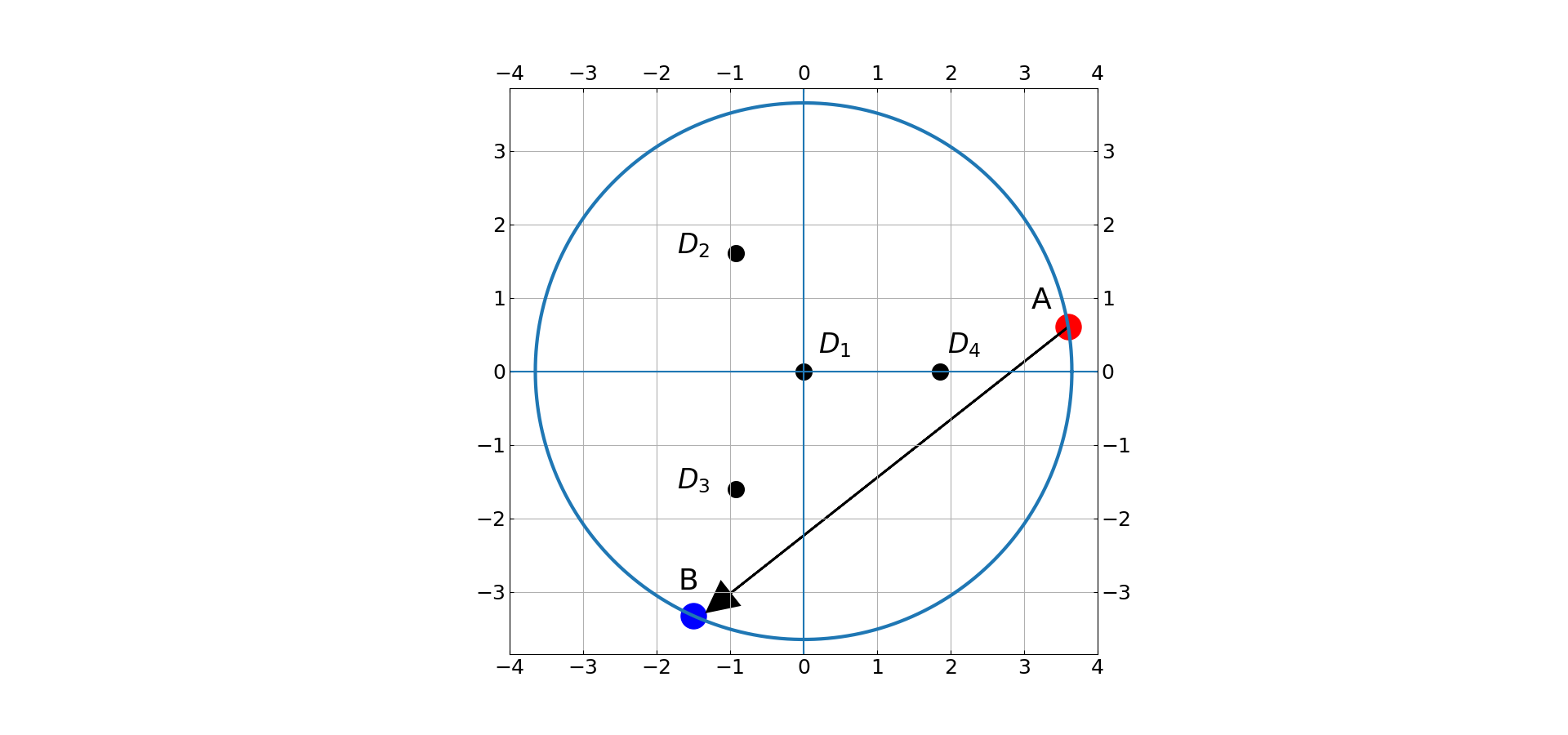
Figure 6: Top view of the WCD tank for a muon entering horizontally through point A and leaving through B. The central detector ($D_{1}$) and the surrounding detectors ($D_{2},D_{3},D_{4}$) are also shown.

A graph of the brightness of Cherenkov images versus their angular locations for this case is shown in Figure 7. The brightness of the muon image at each point in its track has been normalized with respect to its brightness at the entry point $A$ as seen by the central detector. The information in this graph could be recovered from a static digital camera image; a line of variable brightness that encodes the variation of brightness of Cherenkov images with their corresponding angular locations. Note that detector 2 in this case will not see an RID, because this detector is never inside the Cherenkov cone of the muon. The other 3 detectors, however, will each record an RID event. It can also be seen from Figure 7 that none of the light curves shows a strong inverse square dependence on the distance of the Cherenkov images of the muon from the detector. This is primarily attributed to the ratio of the perpendicular distance between the detector and the muon track to the total length of the muon track. The higher this ratio is, the greater the distance dependence of the images. For a typical WCD, all of the distances tend to be of the order of a meter, whereas for a typical Imaging Atmospheric Cherenkov Telescope (IACT), the dynamic range of distances changes from meters to hundreds of kilometers, making the distance dependence of Cherenkov images relatively modest for WCDs when compared to IACTs (Nemiroff & Kaushal, 2020).

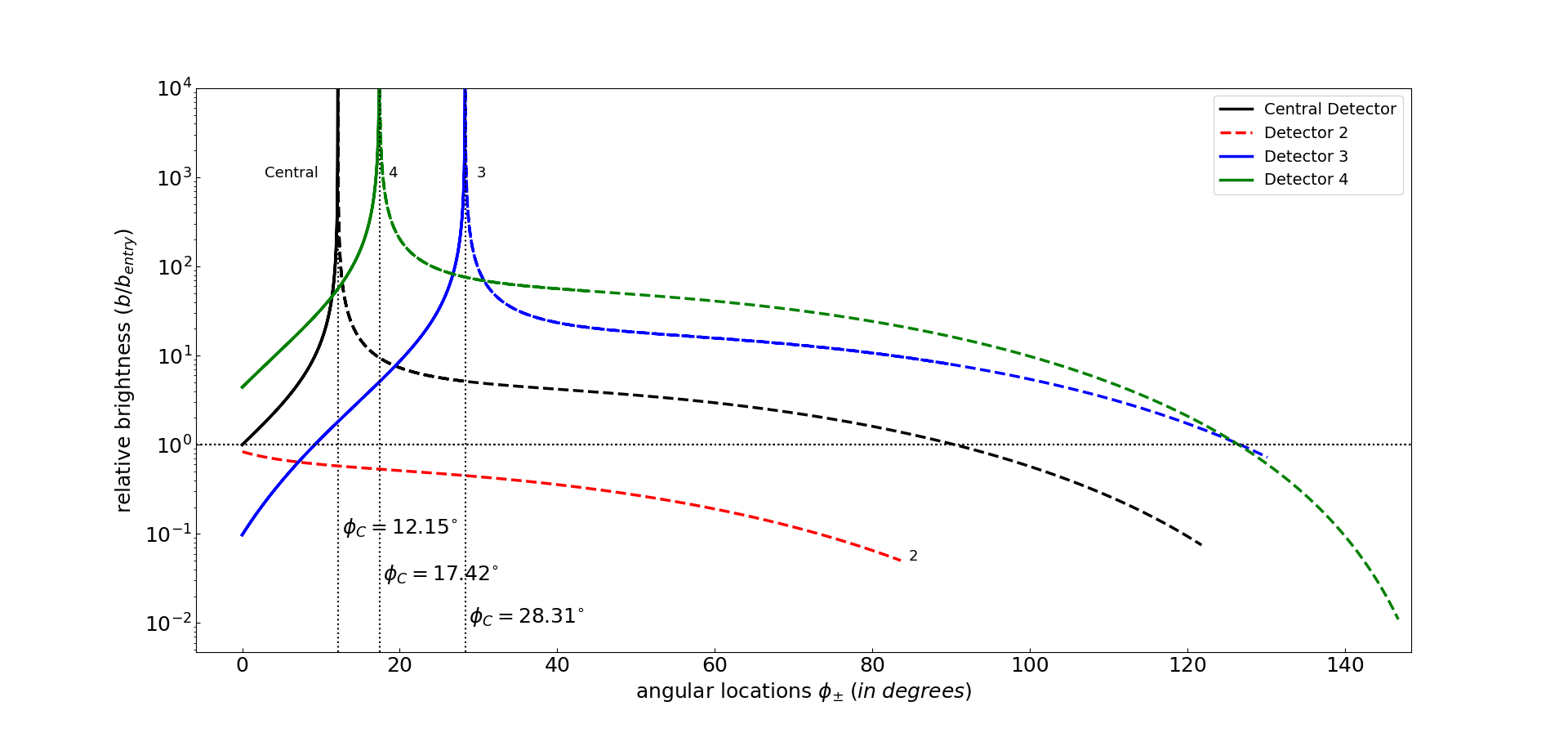
Figure 7: A plot of relative brightness vs angular locations $\phi_{\pm}$ of Cherenkov images of a muon entering the WCD horizontally. The dashed curve corresponds to the image going towards the exit point B, while the solid curve represents the image going back towards the entry point A.

A video detector in this case will see the development of Cherenkov images along the muon track with time. Data extracted from the resulting video would show the angular positions of the images with time as shown in Figure 8. A graph of the distances of the Cherenkov images of muon from its point of entry versus total time is shown in Figure 9. The information on this graph would only be discernible from a high-speed video detector. A PMT in this case will record only the light curve shown in Figure 10.

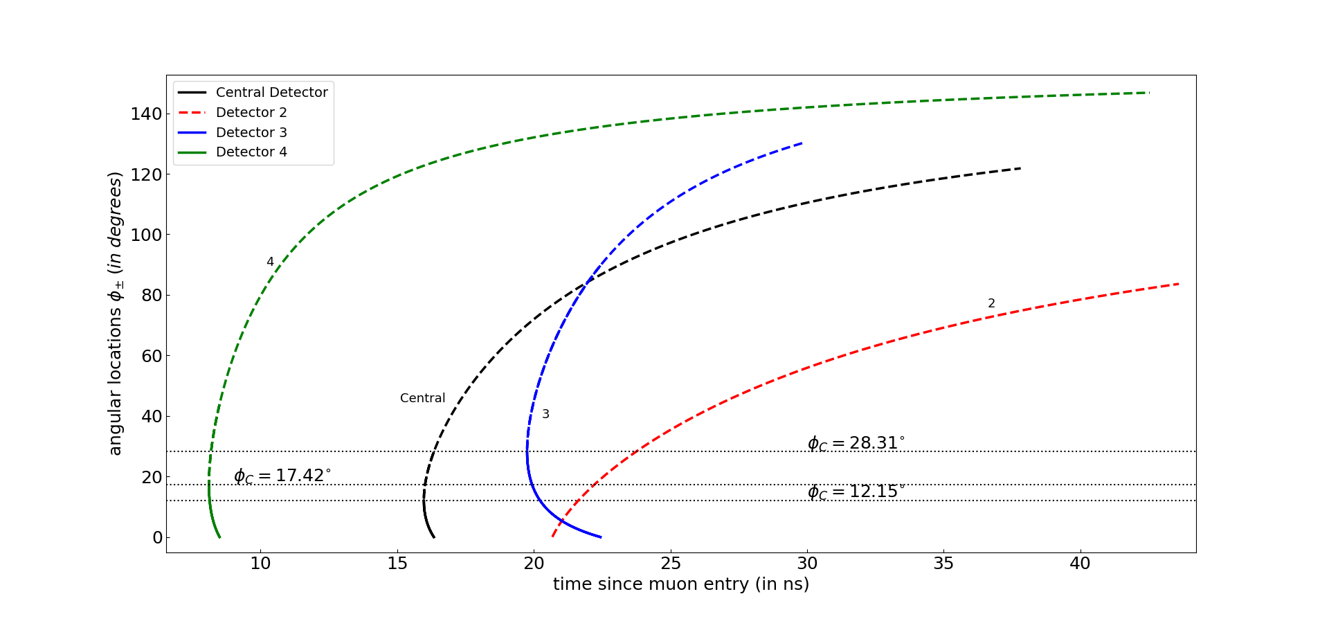
Figure 8: A plot of angular positions of images versus total time for a muon entering the water tank horizontally. The short solid curves depict Cherenkov images moving back towards the entry point A. The long dashed curves depict images moving forward towards the exit point B. The angle $\phi_{C}$ is the critical angle where each detector sees the first RID and it corresponds to the critical distance $x_{C}$. The figure also shows the relative closeness of the first RID locations ($x_{C}$) to the entry point. The shorter the solid curve, the closer $x_{C}$ is to the point of entry of muon.

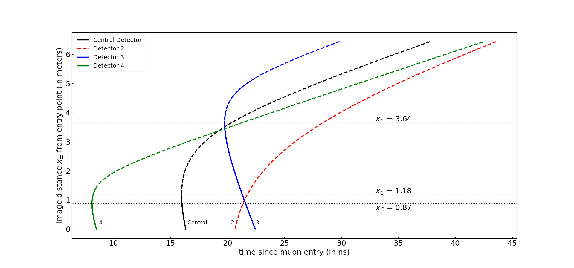
Figure 9: A plot of the distances of the Cherenkov images of the muon from the entry point $A$ versus the total time since the muon entered the tank horizontally.

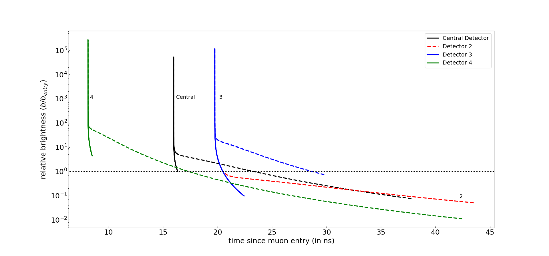
Figure 10: A plot of relative image brightness versus time for a muon entering the WCD horizontally. Note that the Cherenkov images of the same muon track will appear to different detectors at different times with different relative brightness during its entire path inside the WCD. At 22 ns, in total five Cherenkov images of different brightness will be visible collectively to all the detectors.

From inspection of Figure 10, it is clear that the first RID pair of Cherenkov images appears with high brightness (formally infinite) and fades quickly. The two images disappear at different times with respect to the different detectors. The one detector in this example that does not see an RID never sees the single Cherenkov image appear as bright as its pair-counterparts, as observed by other detectors. Also, the solo Cherenkov image this detector sees moves monotonically from $A$ to $B$.

3.3 Incidence at an Arbitrary Angle

More realistically, consider a muon entering the WCD at some point $A$ on the top and leaving the bottom through a different point $B$. As delineated in Eq. 1, the muon’s track makes an angle $\theta$ with respect to the vertical.

The muon travels in a straight line through the WCD at speed $v$. The ground point $B$ may or may not be inside the tank, but the muon trajectory itself will always have the same $\theta$ as it had at point $A$. The muon will trigger Cherenkov radiation when in the tank. Each detector inside the WCD will see this Cherenkov radiation but is not guaranteed to see an RID. The recording of RID by any detector depends on a variety of parameters including but not limited to $\theta$, $L$ and $\alpha$ as indicated in Eq. 1. The apparent heights of the Cherenkov images are given by Eq. 4.

We now consider a very specific example chosen to highlight generic features of RID in WCDs. In this example, the muon (or any charged particle) enters the top of the tank at $A=(2.4,2.4,H)$ with $\theta=20^{\circ}$ and strikes the ground at $B=(0.79,2.68,0)$ which is inside the tank. A graph of image heights from ground $z_{\pm}$ versus the total time $t_{total}$ is shown in Figure 11.

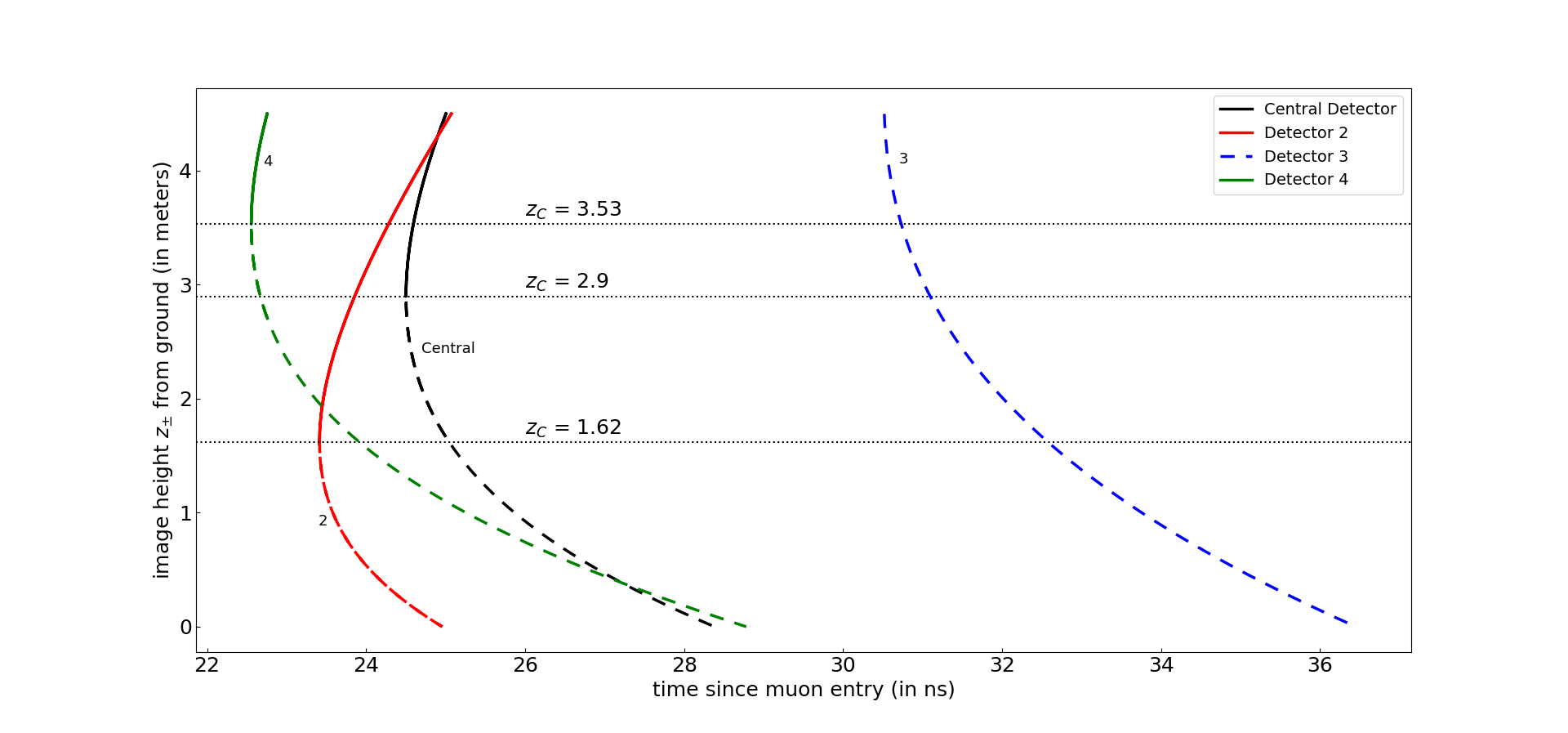
Figure 11: A plot of image heights versus time for a muon entering the tank with the example oblique trajectory given in the text. A solid curve represents the Cherenkov image moving upwards while a dashed curve means that the image is moving downwards towards the bottom. The central detector, as well as detectors 2 and 4, all see an RID, but observe it at different heights from the ground and at different times. Detector 3, however, does not see an RID.

Inspection of Figure 11 shows a time offset of approximately 22 ns between when the muon first enters the WCD at point $A$ and when any of the detectors records Cherenkov light from the muon. This time offset is due to the muon travel time from $A$ to the location of the first detected RID plus the Cherenkov light travel time from this RID location to the detector. As all detectors are at different distances from both $A$ and $B$, the time at which each detector sees an RID, is different.

A graph of angular locations $\phi_{\pm}$ of images versus time $t_{total}$ is shown in Figure 12.

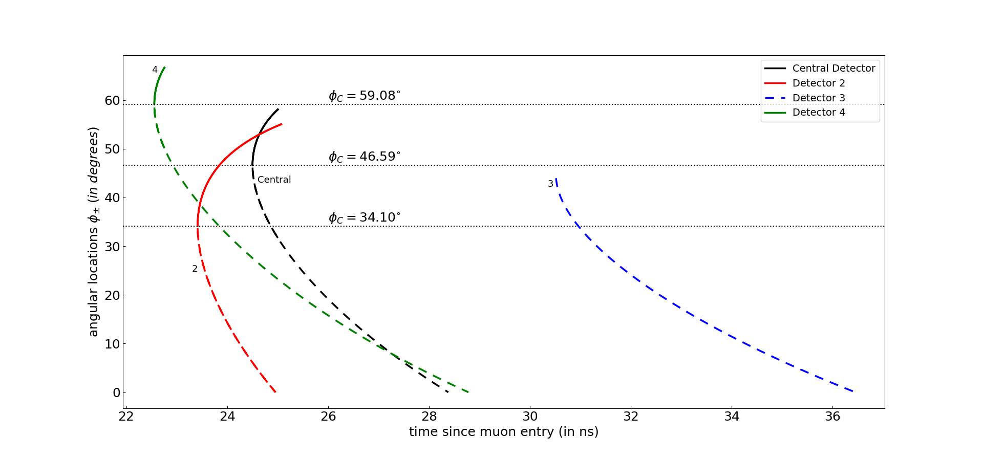
Figure 12: A plot of angular location of Cherenkov images versus total time for a muon entering the WCD at the example oblique trajectory given in the text. Note again that detector 3 does not observe any RID so that the only curve for detector 3 is the dashed one i.e. this detector will see the muon image first at 30.52 ns and last at 36.45 ns.

Inspection of Figure 12 shows that $t_{total}$ is frequently double-valued with respect to $\phi$. For detectors having double-valued curves, the muon is seen for the first time when $z=z_{C}$ i.e. when the first RID is seen. An RID thus produces the first light observed by the detector. Also note that only detector 3 sees a Cherenkov image move classically from point $A$ to point $B$, but only after the other three detectors have stopped observing it.

A graph of relative image brightness versus time for all the four detectors is shown in Figure 13. From this plot, it can be deconvolved what a PMT will record. Figure 13 shows that at roughly 25 ns after the muon enters the tank, three out of four video detectors will collectively observe five images of the same muon as opposed to the conventional notion of observing three images, one for each detector. Each of these five images will stop appearing at different times.

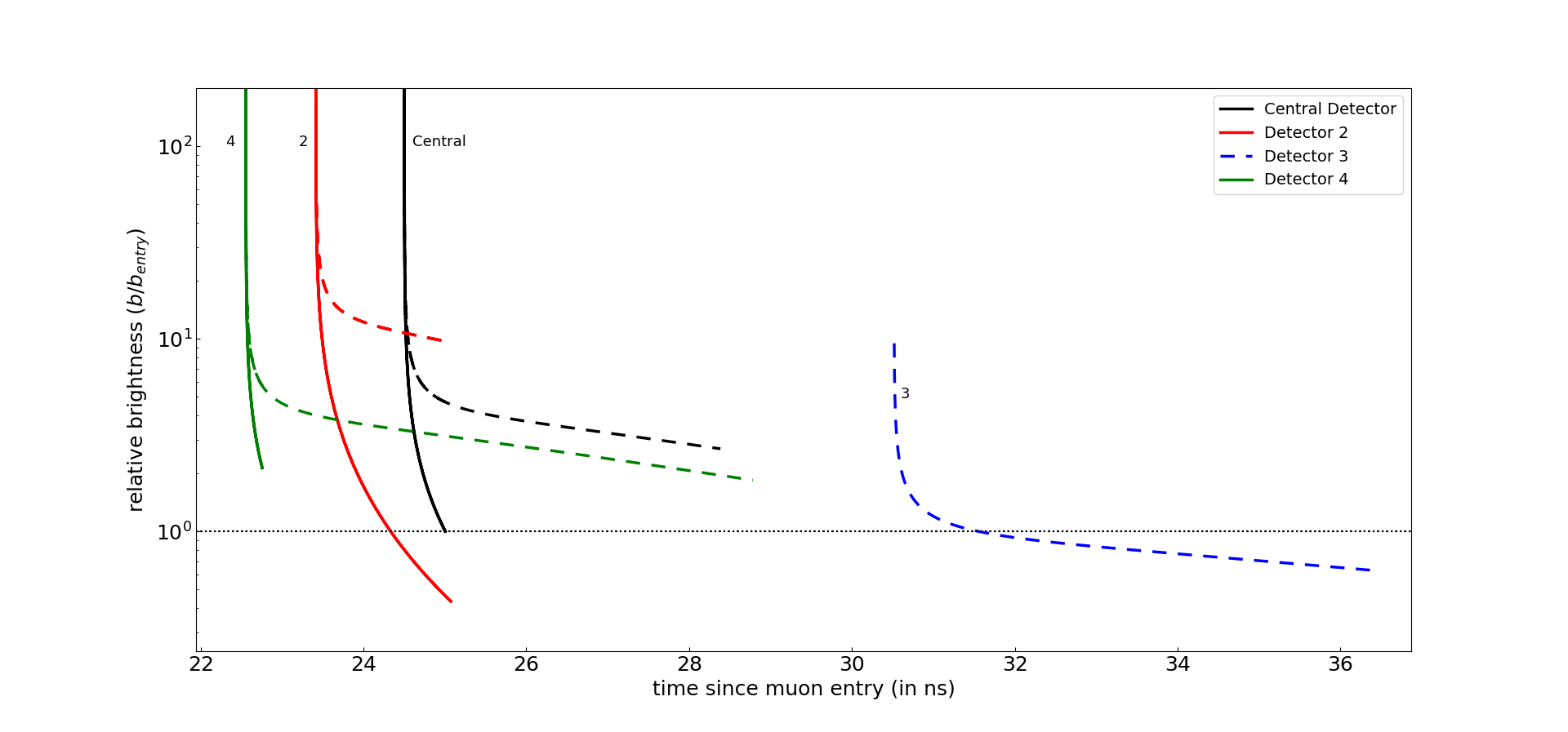
Figure 13: A plot of relative Cherenkov image brightness versus total time for a muon entering the WCD at the example oblique angle. Note that detector 3 starts measuring the brightness of the single Cherenkov image it sees only after the Cherenkov images recorded by the other three detectors have disappeared.

Finally, a graph of relative brightness vs angular locations as observed by all the four detectors is shown in Figure 14. For the detectors that see an RID, the graph shows sharp peaks in the brightness of each image when $z=z_{c}$, which corresponds to $v_{r}=c_{w}$. These peaks correspond to when the Cherenkov images appear for the very first time to each detector. The top Cherenkov image disappears when it reaches the upper lid of the tank at $A$, while the bottom image disappears when it hits the ground at $B$.

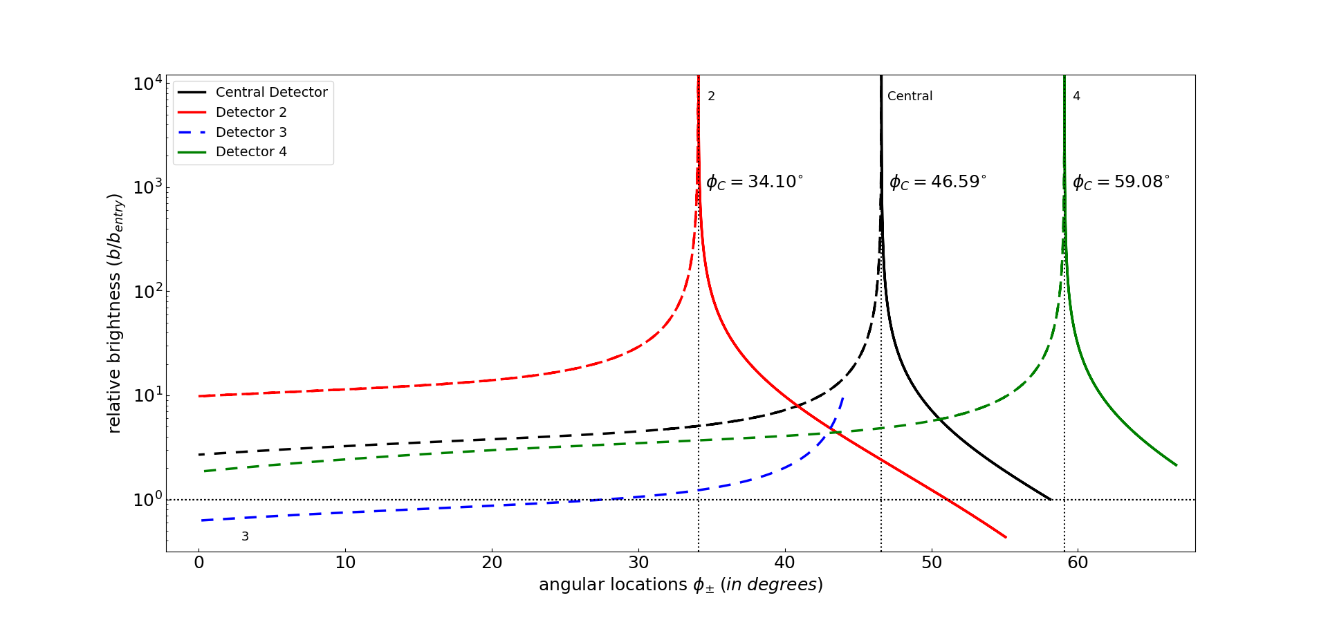
Figure 14: A plot of relative brightness versus angular locations of Cherenkov images of the muon entering the tank at the example oblique angle. An angle $\theta=0^{\circ}$ here corresponds to the detector looking directly towards the entry point $A$.

4 Monte Carlo Simulation: Fraction of Muons Showing an RID Event in a HAWC-Like Detector

Monte Carlo simulation were performed to find the relative fraction of charged, relativistic particles entering a HAWC-like WCD that can cause an RID effect visible to at least one of the internal detectors. Two different algorithms were employed to find this fraction, with both returning similar results. In both algorithms, a cylindrical WCD tank was assumed having radius $R$ and height $H$.

The first algorithm was written in FORTRAN and is shown in Appendix A.1. In this algorithm, muons were assumed to pass through the ground at a random location within three $R$ of the center of the cylindrical WCD. This location, labeled $B$, was then associated with a randomly chosen azimuthal angle $\phi$ relative to an $x$-axis connecting to the center of the bottom of the WCD, and then associated with a randomly chosen zenith angle $\theta$. Given $R$, $\phi$ and $\theta$ for ground location $B$, the muon’s three-dimensional path was uniquely determined. Paths that did not intersect the WCD were discarded. Paths that did intersect the WCD were then assumed to model the muon moving with a downward component through the WCD. The location $A$ where the muon entered the WCD was found. The Cherenkov cone angle $\beta$ was extended from $A$ downward to see if any detectors were inside. The fraction of interior paths to total paths was then computed.

A second algorithm was independently conceived and coded in C++ by the other author and is shown in Appendix A.2. In this algorithm, muons were assumed to come from all possible directions. A random entry point $A$ was first chosen to be anywhere on the top or walls of the tank. Next, a random exit point $B$ was chosen to be located anywhere on the walls or the bottom of the tank. Then a muon track was constructed passing through these points and going down (The $z$-coordinate of exit point was always less than or equal to the $z$-coordinate of entry point). The distance from the entry point $A$ where the first RID would be seen by at least one of the four HAWC-like PMT detectors was found using equation 7 for that muon track. If that RID location was inside the tank, that particular detector was considered to be showing an RID and that muon track was not checked further for any RIDs by the remaining detectors. This process was repeated for a large number of muon tracks which were then subsequently checked for an RID event by at least one of the four detectors.

The two algorithms were run for $1$ billion muon tracks using parameters describing a HAWC-like WCD as shown in Fig. 2 and Fig. 6. Both algorithms found that of all the muons entering the WCD, between $85$ to $90\%$ would create an RID as seen by at least one detector. This indicates that RID events should be seen in HAWC-like WCDs quite commonly. These codes are available on GitHub under an MIT License and version 1.0 is archived in Astrophysics Source Code Library (ASCL) (Kaushal & Nemiroff, 2020).

5 Discussion

Relativistic Image Doubling (RID) is a simple concept in optics where, as opposed to physical or gravitational lenses, relativistic speed itself creates multiple images of the source (Nemiroff, 2018). RID is an observer effect – the muon does not split, for example – and RID can only be observed when something moves faster than light in a given medium. Surprisingly, perhaps, RID effects are actually quite common on Earth, but typically occur on such a short time scale that they are not noticed. To date, only one RID effect has been reported (Clerici et al., 2016), although recently many more have been hypothesized (see, for example, Nemiroff & Kaushal (2020)).

A common medium where RIDs may be observed is water. Many ground-based high-energy gamma-ray observatories use water to facilitate the creation of Cherenkov radiation caused (liberated) by superluminal particles. However, to the best of our knowledge, none of the science teams that run these experiments have published an analysis that acknowledges the RID effect.

RID has several uniquely defining characteristics. One is that, for a given detector, before an RID is detected, no Cherenkov light at all will be seen. It is not that the Cherenkov images are dim, it is that they are not there. For any one detector, the RID appears suddenly and exactly in the direction of the Cherenkov cone of the descending muon. The line connecting the Cherenkov cone to the detector gives the direction of the RID as seen by the detector. Another defining characteristic is that the RID event, as seen by any given detector, is very bright. This high brightness is recorded even though the Cherenkov track is uniformly bright along its track. The reason the RID appears bright is because the detector receives light from a long section of the uniformly bright track all in a short period of time.

After a video detector records an RID event, two Cherenkov images from the RID could be seen moving along the track of the muon, but in opposite directions. The two images will start with formally infinite angular speed, which drops quickly after appearance. These images will start with the same great brightness, but both will quickly fade, and their relative brightness will diverge from unity. This attribute can be important for identifying and verifying images resulting from RID. In the example case of a horizontally moving muon, this fading is shown in Figure 10.

One of the two Cherenkov images will eventually disappear at the location where the actual muon exited the WCD, while the other Cherenkov image will suddenly disappear at the location where the muon entered. It is interesting to note that the backwards-moving Cherenkov image of the muon is actually observed time-backwards by the detector. Although each Cherenkov image will usually appear to fade as it goes, sometimes a competing brightening effect occurs when an image nears a detector.

One might argue that RID is a trivial effect. Who cares that two images of the same muon track are sometimes visible simultaneously? In our view, as also noted in (Nemiroff & Kaushal, 2020), RID is a novel optical effect caused not by lenses but solely by relativistic kinematics – and so is interesting basic physics even without a demonstrated usefulness. However, discovering and tracking RID effects in WCDs may prove useful. Such observations could add information that better allow muon track locations and orientations to be recovered, or give an independent method of confirming the muon’s trajectory. Studying the basic science of other multiple-imaging optical effects is common practice, for example in gravitational lensing (Nemiroff, 1987; Schneider et al., 1992) and temperature inversions effects in the Earth’s atmosphere (Young, A., 1999).

Why have RID effects remained so obscure? One reason is that they have no classical analog – they depend crucially on the finiteness of the speed of light. Classical thinking may allow scientists to accurately visualize how the muon actually moves through the WCD, but not always how it appears to the detector (Nemiroff & Kaushal, 2020).

RID effects may be thought of as immeasurable by some, because both images fade within nanoseconds, as shown in Figure 13. However, tracking the images for even a short angular distance would be interesting. As computer technology and miniaturization is increasing the frame rate that can be captured, imagers appearing over the past few years are becoming capable of recording sub-nanosecond events (Clerici et al., 2016). These technological innovations raise the possibility of placing video detectors inside WCDs that can resolve RID events in both time and angle. Alternatively, simple digital cameras may be placed that can resolve the Cherenkov images only in angle, leaving the temporal resolution to the PMTs.

There are also attributes of realistic detectors that may obscure RID effects. One is that the detector itself is not just a point – it may be so large that light travel time across its surface is significant when compared to $t_{light}$. Then any light curve that a WCD PMT measures will convolve the size and shape of the PMT, not just geometry inherent to the muon’s path.

Because RID effects will look different to different detectors even for the same muon event, the locations of individual detectors are paramount. Therefore, simply adding together the brightness of different images from multiple PMTs, at the times of the brightness measurements, for example, will typically convolute RID effects beyond recognition. However, a careful reconstruction accounting for the timing of separate RID events as seen by different detectors should be possible that could enhance RID detection and better determine the muon’s real track inside the WCD.

There are many interesting RID and detector-related effects that were deemed too complex to be incorporated in this primarily conceptual work. One such effect is the deceleration of the muon as it moves downward through the WCD. A muon that slows significantly will force $z_{C}$ to occur higher in the tank. Additionally, the size of the detectors may cause a convolution of measurements over the time it takes for light to cross the detector. A full treatment of these effects would likely require more detailed and complex computer modeling, but not change the character of the reported results.

In sum, resolving relativistic image doubling events in time and space would recover a novel type of optics caused not by lenses but by relativistic kinematics alone. Further, tracking simultaneous images as they emerge and diverge in angle, angular speed, and relative brightness could resolve or independently confirm information about the muon’s trajectory, including the brightness along its path as described through equations in Section 2.

As a check on the accuracy of the results, the simulations were computed in different programming languages. NK’s Python and C++ codes are listed first followed by RJN’s FORTRAN code.

.1 FORTRAN Code: Monte Carlo Simulation for fraction of muons showing an RID event

⬇

1

2c Computes fraction of HAWC events that show RID.

3 program fractionRID

4c

5c integer*4, parameter :: n=10

6 integer*4 i, ntot, nRID, n, nmax

7 real*8 c, pi, seed, pin, eps, Cangle

8 real*8 R, H, Rd

9 real*8 xd(4), yd(4), zd(4), th(4)

10 real*8 xg, yg, zg, rg

11 real*8 xs, ys, zs, rs

12 real*8 xm, ym, zm, rm

13 real*8 xe, ye, ze, re

14 real*8 x_ge, y_ge, z_ge

15 real*8 x_de(4), y_de(4), z_de(4), r_de(4)

16 real*8 top, bot

17 character*3 before, now, RID

18c Constants

19 nmax=1000000000

20 c=3.0d8

21 pi=dacos(-1.0d0)

22 seed=2.8d0

23 eps=0.1d0

24 Cangle=dacos(1.0d0/1.33d0)*(180.0d0/pi)

25 write (*,*) ’ Input seed, please: ’

26 read (*,*) seed

27c R=radius of tank (meters)

28c H=height of tank (m)

29c Source: https://www.sciencedirect.com/

30c science/article/pii/S0273117713001695?via%3Dihub

31 R=7.30d0/2.0d0

32 H=4.5d0

33c Ground dist. to detectors (check)

34 Rd=7.3d0/4.0d0

35 Rd=1.850d0

36c Location of four ground detectors

37 xd(1)=0.0d0

38 yd(1)=0.0d0

39 zd(1)=0.0d0

40 xd(2)=-Rd

41 yd(2)=0.0d0

42 zd(2)=0.0d0

43 xd(3)=Rd*cos(pi/3.0d0)

44 yd(3)=Rd*sin(pi/3.0d0)

45 zd(3)=0.0d0

46 xd(4)=Rd*cos(pi/3.0d0)

47 yd(4)=-Rd*sin(pi/3.00)

48 zd(4)=0.0d0

49c

50 ntot=0

51 nRID=0

52c ********************

53c Grand loop over muons

54c ********************

55 do 700 n=1, nmax

56c Location muon hits ground

57 xg=3.0d0*R*(2.0d0*pin(seed) - 1.0d0)

58 yg=3.0d0*R*(2.0d0*pin(seed) - 1.0d0)

59 zg=0.0d0

60 rg=sqrt(xg**2 + yg**2)

61 if (rg.ge.5.0d0*R) goto 700

62c Direction muon arrived on sky

63 200 xs=(2.0d0*pin(seed) - 1.0d0)

64 ys=(2.0d0*pin(seed) - 1.0d0)

65 zs=pin(seed)

66 phi=atan(ys,xs)

67c Angular direction of muon

68 phi=2.0d0*pi*pin(seed)

69 theta=acos(zs)

70c Horizon dimming

71 if (pin(seed).gt.zs**2) goto 200

72c

73c ********************** Find where muon enters tank ***

74c

75 xm=xg

76 ym=yg

77 zm=zg

78 rm=sqrt(xm**2 + ym**2)

79c Is muon in the tank?

80 now=’out’

81 if (rm.lt.R.and.zm.lt.H) now=’in’

82c Step the photon back along track

83 300 xm=xm + xs*eps

84 ym=ym + ys*eps

85 zm=zm + zs*eps

86 rm=sqrt(xm**2 + ym**2)

87c write (*,310) xm/R, ym/R, zm/H, rm/R

88c310 format (2x, 4(f7.4, 3x))

89c If muon missed tank try again

90c if (rm.gt.3.0d0*R) write (*,*) ’ Muon missed tank: wide’

91 if (rm.gt.3.0d0*R) goto 700

92c if (zm.gt.H) write (*,*) ’ Muon missed tank: high’

93 if (zm.gt.H) goto 700

94 before=now

95c

96 now=’out’

97 if (rm.lt.R.and.zm.lt.H) now=’in’

98c if (before.eq.’out’.and.now.eq.’in’) write (*,*) "In"

99c If muon left tank then analyze

100c if (before.eq.’in’.and.now.eq.’out’) write (*,*) "Out"

101 if (before.eq.’in’.and.now.eq.’out’) goto 500

102 goto 300

103

104c The muon has just entered the tank

105c Three points: g, e, d

106c For ground, entry, detector

107c Find the vertex angles

108 500 xe=xm

109 ye=ym

110 ze=zm

111 re=rm

112c write (*,*)

113c write (*,*) ’ xm / R = ’, xm/R

114c write (*,*) ’ ym / R = ’, ym/R

115c write (*,*) ’ zm / H = ’, zm/H

116c write (*,*) ’ rm / R = ’, rm/R

117c write (*,*) ’ rg / R = ’, rg/R

118c

119 x_ge=xg - xe

120 y_ge=yg - ye

121 z_ge=zg - ze

122 r_ge=sqrt(x_ge**2 + y_ge**2 + z_ge**2)

123c write (*,*) ’ phi = ’, phi*(180.0d0/pi)

124c write (*,*) ’ theta = ’, theta*(180.0d0/pi)

125c write (*,*)

126c

127 RID=’no’

128 ntot=ntot + 1

129 do 600 i=1, 4

130 x_de(i)=xd(i) - xe

131 y_de(i)=yd(i) - ye

132 z_de(i)=zd(i) - ze

133 r_de(i)=sqrt(x_de(i)**2 + y_de(i)**2 + z_de(i)**2)

134c

135 top=x_ge*x_de(i) + y_ge*y_de(i) + z_ge*z_de(i)

136 bot=r_ge * r_de(i)

137 th(i)=acos(top/bot)*(180.0d0/pi)

138c write (*,*) ’ th(i) = ’, th(i)

139 if (th(i).lt.Cangle) RID=’yes’

140 600 continue

141 if (RID.eq.’yes’) nRID=nRID + 1

142 700 continue

143c

144 write (*,*) ’ nRID, ntot = ’, nRID, ntot

145 write (*,*) ’ RID fraction = ’, float(nRID)/float(ntot)

146

147c Stop the madness.

148 999 stop

149 end

150c

151c*******************************************************

152c

153c Subroutine that uses pi**n algorithm.

154 real*8 function pin(pseed)

155 implicit real*8 (a-h,o-z)

156c

157 pi=dacos(-1.0d0)

158 pseed=pseed*pi

159 if (pseed.gt.10.0d0) pseed=pseed/10.0d0

160 pin=pseed*10000.0d0 - int(pseed*10000.0d0)

161c

162 return

163 end

.2 PYTHON Code: Simulation for horizontal incidence of muon

⬇

1

2

3#!/usr/bin/env python

4#coding: utf-8

5

6#Import Libraries

7import matplotlib.pyplot as plt

8from numpy import sin, cos, sqrt, pi, linspace, arange, deg2rad, rad2deg, array, zeros

9from numpy import arcsin, arccos,sort, argsort, argwhere, argmin, argmax, interp, concatenate

10from scipy.spatial import distance

11import warnings

12from numpy import linalg as LA

13warnings.simplefilter(’ignore’)

14

15#Initialize Parameters

16n = 1.33 #------------------------------------ Refractive index of medium

17c = 299792458/n #----------------------------- Speed of light in medium

18R = 7.3/2 #----------------------------------- Radius of tank

19v = n * c #----------------------------------- Particle Speed

20times = linspace(1e-11,1e-7,200000)

21c1 = (0, 0, 0) #------------------------------ Central PMT number 1

22c2 = (1.85*cos(2*pi/3) , 1.85*sin(2*pi/3), 0) # Non-Radial PMT number 2

23c3 = (1.85*cos(4*pi/3) , 1.85*sin(4*pi/3), 0) # Non-Radial PMT number 3

24c4 = (1.85*cos(0 ) , 1.85*sin(0 ), 0) # Radial PMT number 4

25xA,xB,h= 3.6,-1.5, 0.5

26A = array( [xA , sqrt(R**2-xA**2), h] ) #--- Entry Point of muon

27B = array( [xB , -sqrt(R**2-xB**2), h] ) #--- Exit point of muon

28AB = B-A

29nAB = LA.norm(AB) #-----------------------------Muon path length

30den = c*c - v*v

31print(’A : ’, A)

32print(’B : ’, B)

33

34

35#Bird’s View of tank

36plt.figure(figsize=(10,8))

37angs = linspace(0,6.28,1000)

38xs,ys = R*cos(angs), R*sin(angs)

39plt.plot(xs,ys,lw=3)

40plt.scatter(A[0],A[1],c=’r’,s=500)

41plt.scatter(B[0],B[1],c=’b’,s=500)

42plt.scatter(c1[0],c1[1],c=’k’,s=200)

43plt.scatter(c2[0],c2[1],c=’k’,s=200)

44plt.scatter(c3[0],c3[1],c=’k’,s=200)

45plt.scatter(c4[0],c4[1],c=’k’,s=200)

46plt.axhline(0)

47plt.axvline(0)

48plt.axis(’scaled’)

49plt.arrow(A[0],A[1],B[0]-3.1,B[1]-0.3,head_width=0.4,head_length=0.4,fc=’k’,ec=’k’,lw=2)

50plt.text(A[0]-0.5,A[1]+0.25, "A", fontsize=26)

51plt.text(B[0]-0.2,B[1]+0.35, "B", fontsize=26)

52plt.text(c1[0]+0.2,c1[1]+0.25, "$D_1$", fontsize=24)

53plt.text(c2[0]-0.8,c2[1], "$D_2$", fontsize=24)

54plt.text(c3[0]-0.8,c3[1], "$D_3$", fontsize=24)

55plt.text(c4[0]+0.1,c4[1]+0.25, "$D_4$", fontsize=24)

56plt.xlim(-R-0.2,R+0.2)

57plt.ylim(-R-0.2,R+0.2)

58plt.xticks(arange(-4.0,4.1,1))

59plt.tick_params(axis=’both’, direction=’in’, labelsize=18)

60plt.tick_params(labeltop=True, labelright=True, labelbottom=True)

61plt.tick_params(labelleft=True, bottom=True, top=True, left=True, right=True)

62plt.grid(True)

63plt.show()

64

65

66#Necessary functions

67#Calculate brightness at the muon entry point

68def entry_brightness(L,c,v,alpha,den):

69 tt = L/c

70 aterm = (c*c*tt*v-L*v*v*cos(alpha))

71 bterm = (v*v*( -L*L*v*v + c*c*L*L + c*c*tt*tt*v*v - 2*c*c*L*tt*v*cos(alpha) + L*L*v*v*cos(alpha)**2))

72 xp = (aterm + sqrt(bterm)) / den

73 cterm = (c*c*v)

74 dterm = (c*c*v*v*v*(tt*v-L*cos(alpha)))

75 vp = (cterm + (dterm/sqrt(bterm))) / den

76 kp = sqrt( L*L + xp*xp - 2*L*xp*cos(alpha) )

77 betap = alpha

78 vtp = vp*sin(betap)

79 omegap = vtp / kp

80 bp = abs(omegap/(kp**2))

81 return bp

82

83def sec(x):

84 return 1/cos(x)

85def tan(x):

86 return sin(x)/cos(x)

87

88#Different plotting scenarios

89def plus_t_vs_x (a, b, color, label):

90 plt.plot(a, b, c=color, ls=’-’ , lw=2.5, label=label)

91def minus_t_vs_x(a, b, color, label):

92 plt.plot(a, b, c=color, ls=’--’, lw=2.5, label=label)

93def both_t_vs_x (a1, b1, a2, b2, color, label):

94 plt.plot(a1, b1, c=color, ls=’-’ , lw=2.5, label=label)

95 plt.plot(a2, b2, c=color, ls=’--’, lw=2.5)

96 plt.xlabel(r’time since muon entry (in ns)’,fontsize=18)

97 plt.ylabel(r’image distance $x_{pm}$ from entry point (in meters)’, fontsize=18)

98 plt.axhline(xc, c=’k’, ls=’:’)

99

100def plus_t_vs_b (a, b, color, label):

101 plt.plot(a, b, c=color, ls=’-’, lw=2.5, label=label)

102def minus_t_vs_b(a, b, color, label):

103 plt.plot(a, b, c=color, ls=’--’, lw=2.5, label=label)

104def both_t_vs_b (a1, b1, a2, b2, color, label):

105 plt.plot(a1, b1, c=color, ls=’-’ , lw=2.5, label=label)

106 plt.plot(a2, b2, c=color, ls=’--’, lw=2.5)

107 plt.axhline(1,c=’k’,ls=’:’)

108 plt.xlabel(r’time since muon entry (in ns)’,fontsize=18)

109 plt.ylabel(r’relative brightness ($b/b_{entry}$)’, fontsize=18)

110 plt.yscale(’log’)

111 plt.ylim(1e-2,1e+4)

112

113def plus_t_vs_ang(a, b, color, label):

114 plt.plot(a, b, c=color, ls=’-’, lw=2.5, label=label)

115def minus_t_vs_ang(a, b, color, label):

116 plt.plot(a, b, c=color, ls=’--’, lw=2.5, label=label)

117def both_t_vs_ang(a1, b1, a2, b2, color, label):

118 plt.plot(a1, b1, c=color, ls=’-’ , lw=2.5, label=label)

119 plt.plot(a2, b2, c=color, ls=’--’, lw=2.5)

120 plt.axhline(phic, c=’k’, ls=’:’)

121 plt.xlabel(r’time since muon entry (in ns)’,fontsize=18)

122 plt.ylabel(r’angular locations $\phi_{pm}\;(in\;degrees)$’,fontsize=18)

123

124def plus_b_vs_ang(a, b, color, label):

125 plt.plot(a, b, c=color, ls=’-’, lw=2.5, label=label)

126def minus_b_vs_ang(a, b, color, label):

127 plt.plot(a, b, c=color, ls=’--’, lw=2.5, label=label)

128def both_b_vs_ang(a1, b1, a2, b2, color, label):

129 plt.plot(a1, b1, c=color, ls=’-’ , lw=2.5, label=label)

130 plt.plot(a2, b2, c=color, ls=’--’, lw=2.5)

131 plt.axvline(phic, c=’k’, ls=’:’)

132 plt.axhline(1,c=’k’,ls=’:’)

133 plt.xlabel(r’angular locations $\phi_{pm}\;(in\;degrees)$’,fontsize=18)

134 plt.ylabel(r’relative brightness ($b/b_{entry}$)’, fontsize=18)

135 plt.yscale(’log’)

136 plt.ylim(1e-2,1e+4)

137

138

139#Computations and plotting

140plt.figure()

141plotme = ’t vs b’ #---------Plot type selection

142#plotme = ’t vs x’

143#plotme = ’t vs ang’

144#plotme = ’b vs ang’

145detector_coordinates = [c1,c2,c3,c4]

146colors = [’k’,’r’,’b’,’g’]

147detectors = [1,2,3,4]

148labels = [’Central Detector’, "Detector 2",’Detector 3’,’Detector 4’]

149

150for D, color, detector, mylabel in zip(detector_coordinates, colors, detectors, labels):

151

152 print("==============================================")

153 print("Detector ", detector)

154 AD = D - A

155 BD = D - B

156 L = LA.norm(AD)

157 alpha = arccos((sum(AD*AB))/(L*nAB)) #-Angle between detector and muon track through entry point A

158 xc = L*cos(alpha) - (c*L*sin(alpha))/sqrt(-den) #-Critical height

159 print(’XC: ’,round(xc,3), " m")

160 T,XP,XM,BP,BM,PHIP,PHIM = [],[],[],[],[],[],[]

161

162 for iii,t in enumerate(times):

163

164 x = v*t #------------Distance traveled by muon in time t

165 ratio = x/nAB

166 X = array([ (1-ratio)*A[0] + ratio*B[0] , (1-ratio)*A[1] + ratio*B[1] , h ])

167 AX,DX = X - A, X-D

168 k = sqrt(L*L+x*x-2*L*x*cos(alpha)) #--Distance between detector and muon at time t

169 t1,t2 = t, k/c

170 tt = t1 + t2 #-----------------Total time taken by detector to see the muon

171

172 aterm = (c*c*tt*v-L*v*v*cos(alpha))

173 bterm = (v*v*( -L*L*v*v + c*c*L*L + c*c*tt*tt*v*v - 2*c*c*L*tt*v*cos(alpha) + L*L*v*v*cos(alpha)**2))

174 xp = (aterm + sqrt(bterm)) / den #------Distance of first cherenkov image from entry point A

175 xm = (aterm - sqrt(bterm)) / den #------------------second----------------------------------

176

177 cterm = (c*c*v)

178 dterm = (c*c*v*v*v*(tt*v-L*cos(alpha)))

179 vp = (cterm + (dterm/sqrt(bterm))) / den #----Velocity of first cherenkov image

180 vm = (cterm - (dterm/sqrt(bterm))) / den #----------------second---------------

181

182 kp = sqrt( L*L + xp*xp - 2*L*xp*cos(alpha) ) #---Distance of first cherenkov image from detector

183 km = sqrt( L*L + xm*xm - 2*L*xm*cos(alpha) ) #---------------second-----------------------------

184

185 betap = pi - arccos( (xp*xp + kp*kp - L*L) / (2*xp*kp) )

186 betam = pi - arccos( (xm*xm + km*km - L*L) / (2*xm*km) )

187

188 vtp = vp*sin(betap) #------Transverse velocity of first cherenkov image

189 vtm = vm *sin(betam ) #-----------------------------second---------------

190 omegap = vtp / kp

191 omegam = vtm / km

192 bp,bm = abs(omegap/(kp**2)), abs(omegam/(km **2)) #------Brightness of first and second cherenkov images

193

194 phip = arccos( (L*L + kp*kp - xp*xp ) / (2*L*kp) ) #----Angular location of images as seen by detector

195 phim = arccos( (L*L + km*km - xm*xm ) / (2*L*km) ) #----------------------------do--------------------

196

197 XP.append(xp); XM.append(xm); BP.append(bp); BM.append(bm)

198 PHIP.append(rad2deg(phip)); PHIM.append(rad2deg(phim)); T.append(tt)

199

200 XP, XM, BP, BM, T, PHIP, PHIM = array(XP), array(XM), array(BP), array(BM), array(T), array(PHIP), array(PHIM)

201 TT = T * 1e+9 #------Convert time in nanoseconds

202 conp = [(XP>=0) & (XP<=nAB)] #---Consider only the images inside the tank

203 conm = [(XM>=0) & (XM<=nAB)] #----------------do-------------------------

204 pluslen = len (XP[conp])

205 minuslen = len (XM[conm])

206 kc = sqrt( L*L + xc*xc - 2*L*xc*cos(alpha) ) #---Distance between detector & first RID location

207 phic = rad2deg(arccos( (L*L + kc*kc - xc*xc ) / (2*L*kc) )) #--Angular location of first RID

208 if detector==1:

209 Bnorm = entry_brightness(L,c,v,alpha,den) #---Use this to normalize brightness wrt the entry point

210 #---as seen by the central detector

211 if pluslen == 0:

212 if minuslen == 0:

213 print("Images outside tank. Skipping...")

214 else:

215 print(’One image moving towards exit B.’)

216 TT,XM,BM,PHIM = TT[conm], XM[conm], BM[conm]/Bnorm, PHIM[conm]

217 if plotme==’t vs b’ :minus_t_vs_b (a=TT, b=BM, color=color, label=mylabel)

218 elif plotme==’t vs x’ :minus_t_vs_x (a=TT, b=XM, color=color, label=mylabel)

219 elif plotme==’t vs ang’:minus_t_vs_ang(a=TT, b=PHIM, color=color, label=mylabel)

220 elif plotme==’b vs ang’:minus_b_vs_ang(a=PHIM, b=BM, color=color, label=mylabel)

221

222 elif pluslen != 0:

223 if minuslen == 0:

224 print(’One image moving towards entry A.’)

225 TT,XP,BP,PHIP = TT[conp], XP[conp], BP[conp]/Bnorm, PHIP[conp]

226 if plotme==’t vs b’ :plus_t_vs_b (a=TT, b=BP, color=color, label=mylabel)

227 elif plotme==’t vs x’ :plus_t_vs_x (a=TT, b=XP, color=color, label=mylabel)

228 elif plotme==’t vs ang’:plus_t_vs_ang(a=TT, b=PHIP, color=color, label=mylabel)

229 elif plotme==’b vs ang’:plus_b_vs_ang(a=PHIP, b=BP, color=color, label=mylabel)

230 else:

231 print(’Both images moving’)

232 TTm, XM, BM, PHIM = TT[conm], XM[conm], BM[conm]/Bnorm, PHIM[conm]

233 TTp, XP, BP, PHIP = TT[conp], XP[conp], BP[conp]/Bnorm, PHIP[conp]

234 if plotme==’t vs b’ :both_t_vs_b (a1=TTp, b1=BP, a2=TTm, b2=BM, color=color, label=mylabel)

235 elif plotme==’t vs x’ :both_t_vs_x (a1=TTp, b1=XP, a2=TTm, b2=XM, color=color, label=mylabel)

236 elif plotme==’t vs ang’:both_t_vs_ang(a1=TTp, b1=PHIP, a2=TTm, b2=PHIM, color=color, label=mylabel)

237 elif plotme==’b vs ang’:both_b_vs_ang(a1=PHIP, b1=BP, a2=PHIM, b2=BM , color=color, label=mylabel)

238

239plt.tick_params(axis=’both’, direction=’in’, labelsize=18)

240plt.legend(prop={’size’: 14})

241plt.show()

.3 C++ Code: Monte Carlo Simulation for fraction of muons showing an RID event

⬇

1

2#include<iostream>

3#include<cmath>

4#include<cstdlib>

5#include<ctime>

6using namespace std;

7

8double getRandFloat(double min, double max)

9 {

10 return min + (double) rand() / (double) (RAND_MAX/(max-min));

11 }

12

13int getRandInt(long min, long max)

14 {

15 return min + ( (long) rand() / (long) (RAND_MAX/(max-min+1)) );

16 }

17

18

19double getDistance(double a1[], double a2[], long n)

20 {

21 double distance=0.0;

22 for (unsigned int i=0; i<n; i++)

23 distance += pow(a2[i]-a1[i],2.0);

24 return pow(distance,0.5);

25 }

26

27

28double getAngle(double b[], double a[], double c[], long n)

29 {

30 double ab[n], ac[n];

31 double origin[3]={0.0,0.0,0.0};

32 double dotproduct=0.0;

33 for (unsigned int i=0; i<n; i++)

34 {

35 ab[i] = b[i]-a[i];

36 ac[i] = c[i]-a[i];

37 }

38 for (unsigned int i=0; i<n; i++)

39 dotproduct += (ab[i]*ac[i]);

40 return acos (dotproduct/(getDistance(ab,origin,n) * getDistance(ac,origin,n)));

41 }

42

43

44void setCoordinates(long choice, double point[])

45 {

46 double x,y,z,Y;

47 double H=4.5, R=3.65;

48 x = -R + ( (double) rand() / (double) (RAND_MAX/(R+R)) );

49 if (choice==1)

50 {

51 Y = pow(R*R-x*x,0.5);

52 y = -Y + ( (double) rand() / (double) (RAND_MAX/(Y+Y)) );

53 z = H;

54 }

55 else if (choice==2)

56 {

57 z = 0.0 + ( (double) rand() / (double) (RAND_MAX/(H)) );

58 y = pow(R*R-x*x,0.5);

59 int dir = 1 + ( (long) rand() / (long) (RAND_MAX/(2-1+1)) );

60 if (dir==2)

61 y = -y;

62 }

63 else

64 {

65 Y = pow(R*R-x*x,0.5);

66 y = -Y + ( (double) rand() / (double) (RAND_MAX/(Y+Y)) );

67 z = 0;

68 }

69 point[0]=x;

70 point[1]=y;

71 point[2]=z;

72 }

73

74

75int main(int argc , char* argv[])

76 {

77 srand(time(0));

78 const long all_cases=atol(argv[1]);

79 const long pi=3.141597;

80 const double c=299792458.0/1.33, v=1.33*c, H=4.5, R=3.65;

81 const double c1[3] = {0.0, 0.0, 0.0};

82 const double c2[3] = {1.85*cos(2*pi/3) , 1.85*sin(2*pi/3), 0.0};

83 const double c3[3] = {1.85*cos(4*pi/3) , 1.85*sin(4*pi/3), 0.0};

84 const double c4[4] = {1.85*cos(0) , 1.85*sin(0) , 0.0};

85 long counts=0, iter=0;

86 long choice_A, choice_B, flag;

87 double A[3], B[3], X[3];

88 double alpha, nAB, L, xc, ratio;

89

90 while (iter<all_cases)

91 {

92 choice_A = getRandInt(1,2);

93 choice_B = getRandInt(2,3);

94 setCoordinates(choice_A, A);

95 setCoordinates(choice_B, B);

96 while (B[2] > A[2])

97 {

98 choice_A = getRandInt(1,2);

99 choice_B = getRandInt(2,3);

100 setCoordinates(choice_A, A);

101 setCoordinates(choice_B, B);

102 }

103 nAB = getDistance(A,B,3);

104 double detectors[1][4][3] = {{{c1[0],c1[1],c1[2]}, {c2[0],c2[1],c2[2]},

105 {c3[0],c3[1],c3[2]}, {c4[0],c4[1],c4[2]}}};

106 flag = 0;

107 for (int index=0; index<4; index++)

108 {

109 alpha = getAngle(B,A,detectors[0][index],3);

110 L = getDistance(A,detectors[0][index],3);

111 xc = L*cos(alpha) - ( (c*L*sin(alpha)) / (pow(v*v-c*c,0.5)) );

112 ratio = xc/nAB;

113 X[0] = (1-ratio)*A[0]+ratio*B[0];

114 X[1] = (1-ratio)*A[1]+ratio*B[1];

115 X[2] = (1-ratio)*A[2]+ratio*B[2];

116

117 if ( ((X[0]*X[0]+X[1]*X[1])<=R*R) && (X[2]>=0.0) && (X[2]<=H) )

118 {

119 counts+=1;

120 flag = 1;

121 }

122 if (flag==1)

123 break;

124 }

125 iter+=1;

126 }

127

128 cout<<"Total Particles : "<<all_cases<<endl;

129 cout<<"Particles RIDed : "<<counts<<endl;

130 cout<<"Fraction : "<<(double)counts/(double)all_cases<<endl;

131 return 0;

132}

References

- Aab et al. (2015) Aab, A., Abreu, P., Aglietta, M., et al. 2015, ApJ, 802, 111
- Aartsen et al. (2014) Aartsen, M. G., Abbasi, R., Ackermann, M., et al. 2014, Journal of Instrumentation, 9, P03009
- Aartsen et al. (2017) Aartsen, M. G., Ackermann, M., Adams, J., et al. 2017, Journal of Instrumentation, 12, P03012
- Actis et al. (2011) Actis, M., Agnetta, G., Aharonian, F., et al. 2011, Experimental Astronomy, 32, 193
- Aharonian et al. (2006) Aharonian, F., Akhperjanian, A. G., Bazer-Bachi, A. R., et al. 2006, A&A, 457, 899
- Aliu et al. (2009) Aliu, E. et al. 2009, Astroparticle Physics 30, 293
- Arisaka et al. (1984) Arisaka, K., Kajita, T., Kifune, T., et al. 1984, American Institute of Physics Conference Series, 54
- BenZvi (2015) BenZvi, S. 2015, European Physical Journal Web of Conferences, 01003
- Baixeras et al. (2004) Baixeras, C., Bastieri, D., Bigongiari, C., et al. 2004, Nuclear Instruments and Methods in Physics Research A, 518, 188
- Butslov et al. (1963) Butslov, M. M., Medvedev, M. N., Chuvilo, I. V., & Sheshunov, M. V. 1963, Nuclear Instruments and Methods, 20, 263
- Cavaliere et al. (1971) Cavaliere, A., Morrison, P., & Sartori, L. 1971, Science, 173, 525
- Čerenkov (1937) Čerenkov, P. A. 1937, Physical Review, 52, 378
- Clerici et al. (2016) Clerici, M., Spalding, G. C., Warburton, R., et al. 2016, Science Advances, 2, e1501691
- Daum et al. (1997) Daum, A., Hermann, G., Heß, M., et al. 1997, Astroparticle Physics, 8, 1
- Hakkila & Nemiroff (2019) Hakkila, J., & Nemiroff, R. 2019, ApJ, 883, 70
- Hess et al. (1999) Hess, M. et al. 1999, Astroparticle Physics, 11, 363
- Hillas (1982) Hillas, A. M. 1982, J. Phys. G: Nucl. Phys 8, 1475
- Hillas (1985) Hillas, A.M. 1985, 19th International Cosmic Ray Conference (ICRC19), Volume 3, 445
- Holder et al. (2006) Holder, J., Atkins, R. W., Badran, H. M., et al. 2006, Astroparticle Physics, 25, 391
- Kaushal & Nemiroff (2020) Kaushal, N., Nemiroff, R. J. 2020, Relativistic Image Doubling in Water Cherenkov Detectors, 001, Astrophysics Source Code Library, ascl:2005.001
- Lewis (1990) Lewis, D. A. 1990, Experimental Astronomy, 1, 213
- Maier & Holder (2017) Maier, G., & Holder, J. 2017, International Cosmic Ray Conference, 35, 747
- Morrison (1958) Morrison, P. 1958, Il Nuovo Cimento, 7, 858
- Nemiroff (1987) Nemiroff, R. J. 1987, Ph.D. Thesis
- Nemiroff (2015) Nemiroff, R. J. 2015, PASA, 32, e001
- Nemiroff & Zhong (2017) Nemiroff, R. J., & Zhong, Q. 2017, arXiv:1703.05811
- Nemiroff (2018) Nemiroff, R. J. 2018, Annalen der Physik, 530, 1700333
- Nemiroff (2019) Nemiroff, R. 2019, American Astronomical Society Meeting Abstracts #233, 233, #251.01
- Nemiroff & Kaushal (2020) Nemiroff, R. J., & Kaushal, N. 2020, ApJ, 889, 122
- Porter & Weekes (1977) Porter, N. A., & Weekes, T. C. 1977, SAO Special Report, 381, 381
- Rossi (1933) Rossi, B. 1933, Zeitschrift fur Physik, 82, 151
- Sandoval (2013) Sandoval, A. 2013, International Cosmic Ray Conference, 1155
- Schneider et al. (1992) Schneider, P., Ehlers, J., & Falco, E. E. 1992, Gravitational Lenses, XIV, 560 pp. 112 figs.. Springer-Verlag Berlin Heidelberg New York. Also Astronomy and Astrophysics Library, 112
- Tanabashi et al. (2018) Tanabashi, M., Hagiwara, K., Hikasa, K., et al. 2018, Phys. Rev. D, 98, 030001
- Weekes et al. (2002) Weekes, T. C., Badran, H., Biller, S. D., et al. 2002, Astroparticle Physics, 17, 221
- Young, A. (1999) Young, Andrew T. 1999, An Introduction to Mirages https://aty.sdsu.edu/mirages/mirintro.html