Stellar energy loss rates beyond the standard model

Abstract

It is known that the dipole moments of the neutrino lead to important astrophysical and cosmological effects. In this regard, within the context of a $U(1)_{B-L}$ model, we develop and present novel analytical formulas to assess the effects of the anomalous magnetic moment and electric dipole moment of the neutrino on the stellar energy loss rates through some common physical process of pair-annihilation $e^{+}e^{-}\to(\gamma,Z,Z^{\prime})\to\nu\bar{\nu}$. Our results show that the stellar energy loss rates strongly depends on the effective magnetic moment of the neutrino, but also on the parameters which characterize the adopted $U(1)_{B-L}$ model.

I Introduction

At the beginning of the last century, the establishment of the Hertzsprungh-Russell (HR) diagram led quickly to the bases of a stellar evolution theory, which identified mass as the fundamental parameter to determine the structure, nucleosynthesis, mean lifetime, ways of production and release of energy, stability mechanisms and the final product of stars. We now know that massive stars with minimum initial mass of approximately $7M_{\odot}<M<9M_{\odot}$ are the potential precursors of different types of supernovae type I (SN I) with subtypes Ia, Ib, and Ic. The former two being mainly linked to single white dwarfs, moderate mass interacting binaries, whereas the lattest of them seems to be linked to massive Wolf-Rayet stars Kilpatrick2018 . Supernovae type II (SN II), with subtypes IIn, IIP, IIL IIb and IIe are associated with massive stars of initial masses within $10M_{\odot}<M<35M_{\odot}$, resulted from red supergiant stars, most massive white dwarfs and very luminous blue variable stars hendry2006 ; smartt2009 . Each of these SN populations are potential progenitors of neutron stars and black holes.

In a SN event, the violent outburst triggered by the gravitational collapse of a Fe-core of mass approximately $1.3-2M_{\odot}$ toward a neutron star, releases an energy about $E_{\nu}\approx(3-5)\times 10^{53}$ erg in the form of neutrinos and antineutrinos of the three flavors ($\nu_{e},\nu_{\mu},\nu_{\tau}$). The gravitational binding energy of the resulting neutron star corresponds nearly to ($10-15\%$) of the core rest mass. The remaining core-collapsed SN can reach extremely high surface temperatures and densities, e.g. up to $3\times 10^{8}K$ and $\rho\leq 10^{5}gr/cm^{3}$. Therefore, contrary to normal stars where photons can be transported to the surface by radiative or convective processes, neutrinos interact extremely weakly and can easily escape from stellar interiors taking away such amounts of energy. These stellar energy loss rates, which leads to cooling by neutrino emission, are mainly due to purely leptonic processes and weak nuclear reactions. However although large values of temperatures and densities seems to characterize well the final stage of stellar evolution, the former are dominant. Under these conditions, we can identify four main mechanisms of neutrino pair production relevant for the neutrino luminosity beaudet1967 ; dicus1972 ; dicus1976 ; alam1989 ; dicus1977 ; bruenn1985 ; torres2010 ; hernandez2017 :

$$e^{+}e^{-} \rightarrow\nu\bar{\nu}\hskip 8.53581pt\textrm{ (pair-annihilation)},$$ (1)

$$\gamma+e^{\pm} \rightarrow e^{\pm}\nu\bar{\nu}\hskip 8.53581pt\textrm{ ($\nu-$ pair photoproduction)},$$ (2)

$$\gamma^{*} \rightarrow\nu\bar{\nu}\hskip 8.53581pt\textrm{ (plasmon decay)},$$ (3)

$$e^{\pm}+Z \rightarrow e^{\pm}+Z\nu\bar{\nu}\hskip 8.53581pt\textrm{ (bremsstrahlung)}.$$ (4)

Quantify stellar energy loss rates is recognized as a priority scientific knowledge to set constraints on the properties and interaction of light particles dicus1972 ; dicus1976 ; ellis1983 ; bruenn1985 , which give important advances in astrophysics and cosmology tanabashi2018 ; gerbino2017 ; raffelt1996 . Furthermore, one of the most interesting possibilities to use stars as particle physics laboratories is to study the backreaction of the novel energy loss rates implied by the existence of new low-mass particles such as axions payez2015 ; fischer2016 , which remain as candidates to dark matter.

On the other hand, the weak interaction predicts interactions between the neutrino and photon through a non-zero magnetic moment induced via loop corrections of gauge boson. In the minimal extension of the Standard Model (SM) with massive Dirac neutrinos, the diagonal magnetic moment of the neutrino mass eigenestate $\nu_{i}$ is proportional to its mass $m_{i}$ and is given by Fujikawa-MM ; Robert-MM ; Fukugita1-MM ; bugarin2017 :

$$\mu^{ii}_{\nu}=\frac{3eG_{F}m_{i}}{8\sqrt{2}\pi^{2}}=3.2\times 10^{-19}(\frac{m_{i}}{eV})\mu_{B},$$ (5)

where $\mu_{B}$ is the Bohr magneton.

Discoveries of new interactions and/or nonstandard properties of neutrinos could modify the rate at which neutrinos are produced, or they can even carry more, or less energy. In this respect, for instance, the electromagnetic properties of the neutrino, such as the Anomalous Magnetic Moment (AMM) and the Electric Dipole Moment (EDM) have given one of the most sensitive probes of physics beyond the Standard Model (BSM) mohapatra2004 ; bugarin2017 ; ko2019 . These interactions are expected to generate observable effects in astrophysical environments kerimov1992 ; blinnikov1994 ; raffelt1999 ; heger2009 ; giunti2015 . Furthermore, they will be of relevance in cosmology gerbino2017 , and terrestrial neutrino experiments cisneros1971 .

Bounds on the diagonal magnetic moment of the neutrino have been reported as the result of different astrophysical and experimental determinations; for example, Barbieri-MM show that the abscence of high-energy events in the SN1987A neutrino signal puts a higher bound of $\mu_{\nu}\lesssim 10^{-12}\mu_{B}$ at $90\%$. Supernova energy loss studies lead to an upper limit of $\mu_{\nu}\lesssim(1.1-2.7)\times 10^{-12}\mu_{B}$ at $90\%$ according to Kuznetsov-MM . Cooling rates of red giants Raffelt-MM gives a comparable bound of $\mu_{\nu}\lesssim 3\times 10^{-12}\mu_{B}$ at $90\%$, whereas analysis of cooling rates of white dwarfs Blinnikov-MM puts a limit of $\mu_{\nu}\lesssim 10^{-11}\mu_{B}$ at $90\%$. Recent bounds were also obtained for the Borexino experiment Borexino-MM which explores solar neutrinos $\mu_{\nu}\leq 5.4\times 10^{-11}\mu_{B}$ at $90\%$, and the TEXONO Collaboration Texono-MM get $\mu_{\nu}<2.9\times 10^{-11}\mu_{B}$ at $90\%$, etc. All these bounds are reasonably compatible.

Concerning the simplest extensions to the SM, the $U(1)_{B-L}$ model mohapatra1980 ; marshak1980 ; buchmuller1991 ; emam2007 ; khalil2008 take into account an extra $U(1)$ local gauge symmetry carlson1987 , where B and L denote the baryon number and lepton number, respectively. The B-L model basso2009 is attractive due to its relatively simple theoretical structure, as it contains an extra gauge boson $Z^{\prime}$ corresponding to B-L gauge symmetry and an extra SM singlet scalar (heavy Higgs boson $H$). The mass of the additional boson $Z^{\prime}$ is given by the relation $M_{Z^{\prime}}=2v^{\prime}g^{\prime}_{1}$ khalil2008 ; emam2007 ; basso2009 . This boson $Z^{\prime}$ interacts with the leptons, quarks, heavy neutrinos and light neutrinos with interaction strengths proportional to the B-L gauge coupling $g^{\prime}_{1}$. The $U(1)_{B-L}$ model becomes mostly attractive due that can account for dark matter abundance singirala2018 .

It is important to point out that, in the early Universe, from a few femtoseconds after the Big-Bang up to the electroweak scale, period in which the last positrons disappeared, the relevant degrees of freedom are pressure, the energy density, entropy density, and number density. Then, in the B-L model neutrinos are not produced in purely left-handed states, probably the thermally excited degrees of freedom in the early universe would increase, providing constraints on the alternative model. A review of the fundamentals of the minimal B-L model adopted in this paper can be read in bugarin2017 and references therein.

The priority objective of this paper is to study the combined effects of a) the AMM and the EDM of the neutrino, and b) the parameters of the $U(1)_{B-L}$ model on the determination of stellar energy loss rates through the process of pair-annihilation $e^{+}e^{-}\to(\gamma,Z,Z^{\prime})\to\nu_{i}\bar{\nu}_{i}$ with $\nu_{i}=\nu_{e},\nu_{\mu},\nu_{\tau}$. We shall present analytical exact formules for this purpose, and we get the relative emission compared with those of the SM.

With these goals, the paper is organized as follows: Within the context of the $U(1)_{B-L}$ model, in Section II we perform the calculations of the transition amplitude, the total cross-section and the exact determination of the stellar energy loss rates. The relative correction for the stellar energy loss rates with the SM is also shown. In Section III, we present a discussion and our results. Finally, we give our main conclusions in Section IV.

II Stellar energy loss rates through the process $e^{+}e^{-}\to\nu\bar{\nu}$

It is already well known that during the later phases of stellar evolution, once the core bounce and a proton-neutron star forms at the center of the SN explosion, the huge amount of energy of the order of $10^{53}$ ergs is realised in the form of pairs neutrinos and antineutrinos. Evidently, neutrinos of the three flavors with extra freedom degrees such as AMM and EDM would be able to take away more amounts of energy. This is the case of the neutrino involved in the pair-annihilation process $e^{+}e^{-}\rightarrow\nu\bar{\nu}$ given by Eq. (1) which would be an important agent for cooling the collapsed core by neutrino emission.

In our calculations, we incorporate the AMM and the EDM of the neutrino. We also quantify the dependence on these momenta of the stellar energy loss rate through the process of pair-annihilation $e^{+}e^{-}\to(\gamma,Z,Z^{\prime})\to\nu\bar{\nu}$ and on the parameters associated with the $U(1)_{B-L}$ model.

II.1 Amplitudes calculation

We focus now on the calculation of the amplitude for the pair-annihilation:

$$e^{+}\left(p_{1}\right)e^{-}\left(p_{2}\right)\rightarrow(\gamma,Z,Z^{\prime})\to\nu_{i}\left(k_{1},\lambda_{1}\right)\bar{\nu}_{i}\left(k_{2},\lambda_{2}\right),$$ (6)

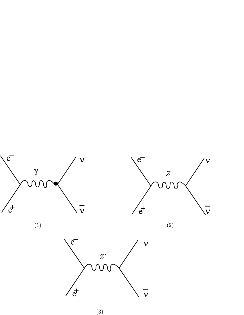
Figure 1: The Feynman diagrams contributing to the process $e^{+}e^{-}\rightarrow(\gamma,Z,Z^{\prime})\to\nu\bar{\nu}$. The dot represents an interaction arising from a effective operator.

with $\gamma$, $Z$, $Z^{\prime}$ exchanges and $\nu_{i}=\nu_{e},\nu_{\mu},\nu_{\tau}$, respectively. Here the $k_{i}$ and $p_{i}$ are the particles quadrimoment and $\lambda_{i}$ is the neutrino helicity. The Feynman diagrams contributing to the process given by Eq. (6) are shown in Fig. 1.

For neutrinos the electric charge is zero and there are no electromagnetic interactions at tree-level between the neutrino field $\nu(x)$ and the electromagnetic field $A^{\mu}(x)$. However, such interactions can arise at the quantum level from loop diagrams at higher order of the perturbative expansion of the interaction. In the one-photon approximation, the electromagnetic interactions of a neutrino field $\nu(x)$ can be described by an effective interaction. In this regard, the electromagnetic properties of any fermion appear in quantum field theory through its interaction with the photon. Thus, the most general expression for the effective vertex of the interaction $\nu\bar{\nu}\gamma$ is given by nieves1982 ; kayser1983 :

$$\Gamma^{\alpha}=eF_{1}(q^{2})\gamma^{\alpha}+\frac{ie}{2m_{\nu}}F_{2}(q^{2})\sigma^{\alpha\mu}q_{\mu}+\dfrac{e}{2m_{\nu}}F_{3}(q^{2})\gamma_{5}\sigma^{\alpha\mu}q_{\mu}+eF_{4}(q^{2})\gamma_{5}(\gamma^{\alpha}-\dfrac{q\hbox to0.0pt{\hss/}q^{\alpha}}{q^{2}}),$$ (7)

where $q^{\mu}$ is the photon momentum, and $F_{1,2,3,4}(q^{2})$ are the electromagnetic form factors of the neutrino. Strictly, the $F_{1,2,3,4}(q^{2})$ form factors are not physical quantities, but in the limit $q^{2}\to 0$ they become quantifiable and related to the static quantities corresponding to Charge Radius, AMM, EDM and the Anapole Moment (AM), respectively giunti2015 ; vogel1989 . In this analysis, we are interested in the AMM and the EDM of the neutrino, which are defined in terms of the $F_{2}\left(q^{2}=0\right)$ and $F_{3}\left(q^{2}=0\right)$ form factors as follows gutierrez2018 :

$$\mu_{\nu}=\frac{m_{e}}{m_{\nu}}F_{2}\left(q^{2}=0\right),\qquad d_{\nu}=\dfrac{e}{2m_{\nu}}F_{3}\left(q^{2}=0\right).$$ (8)

Throughout the rest of the paper, the form factors corresponding to charge radius and the anapole moment are not considered.

Using the couplings between the $Z$, $Z^{\prime}$ bosons with those of the SM fermions given in Table 1 of Appendix A, the respective transition amplitudes are thus given by:

$$i\mathcal{M}_{\gamma} =\bar{u}\left(k_{2},\lambda_{2}\right)\Gamma^{\alpha}\upsilon\left(k_{1},\lambda_{1}\right)\dfrac{-ig_{\mu\nu}}{\left(p_{1}+p_{2}\right)^{2}}\bar{\upsilon}\left(p_{1}\right)ie\gamma_{\mu}u\left(p_{2}\right),$$ (9)

$$i\mathcal{M}_{Z} =\bar{u}\left(k_{2},\lambda_{2}\right)\left(\dfrac{-ig}{\cos{\theta_{W}}}\right)\gamma^{\mu}\frac{1}{2}\left(g_{V}^{\nu}-{g_{A}^{\nu}\gamma}_{5}\right)\upsilon\left(k_{1},\lambda_{1}\right)$$

$$\quad\times\dfrac{-i(g_{\mu\nu}-p_{\mu}p_{\nu}/M_{Z}^{2})}{\left[\left(p_{1}+p_{2}\right)^{2}-M_{Z}^{2}-iM_{Z}\Gamma_{Z}\right]}\bar{\upsilon}\left(p_{1}\right)\left(\dfrac{-ig}{\cos{\theta_{W}}}\right)\gamma^{\nu}\frac{1}{2}\left(g_{V}^{e}-{g_{A}^{e}\gamma}_{5}\right)u\left(p_{2}\right),$$ (10)

$$i\mathcal{M}_{Z^{\prime}} =\bar{u}\left(k_{2},\lambda_{2}\right)\left(\dfrac{-ig}{\cos{\theta_{W}}}\right)\gamma^{\mu}\frac{1}{2}\left(g^{\prime\nu}_{V}-{g^{\prime\nu}_{A}\gamma}_{5}\right)\upsilon\left(k_{1},\lambda_{1}\right)$$

$$\quad\times\dfrac{-i(g_{\mu\nu}-p_{\mu}p_{\nu}/M_{Z^{\prime}}^{2})}{\left[\left(p_{1}+p_{2}\right)^{2}-M_{Z^{\prime}}^{2}-iM_{Z^{\prime}}\Gamma_{Z^{\prime}}\right]}\bar{\upsilon}\left(p_{1}\right)\left(\dfrac{-ig}{\cos{\theta_{W}}}\right)\gamma^{\nu}\dfrac{1}{2}\left(g^{\prime e}_{V}-{g^{\prime e}_{A}\gamma}_{5}\right)u\left(p_{2}\right),$$ (11)

where $u$ and $v$ are the usual Dirac spinors, and the electron and positron helicity indexes have been suppressed since they will be averaged over. The constants $g_{V}^{e}$, $g_{A}^{e}$, $g_{V}^{\nu}$ and $g_{A}^{\nu}$ depend only of the parameters of the $U(1)_{B-L}$ model, that is $\theta_{B-L}$ and $g^{\prime}_{1}$ (see Table 1 of Appendix A).

The squared transition amplitude is derived by the use of Eqs. (9)-(11), resulting:

$$\sum_{s} \left|\mathcal{M}_{\nu\bar{\nu}}\right|^{2}=\dfrac{4\left(4\pi\alpha\right)^{2}}{\sin^{4}{2\theta_{W}}}\Bigg{\{}\dfrac{\sin^{4}{2\theta_{W}}}{\left(4\pi\alpha\right)}\left(\mu_{\nu}^{2}+d_{\nu}^{2}\right)\left(\dfrac{\left(p_{1}\cdot p_{2}+m_{e}^{2}\right)\left(p_{1}\cdot k_{2}+m_{e}^{2}\right)}{\left(p_{1}+p_{2}\right)^{2}}\right)$$

$$+\Bigg{[}\bigg{(}\dfrac{1}{M_{Z}^{2}}\big{(}g_{V}^{e}-g_{A}^{e}\big{)}\big{(}g_{V}^{\nu}+g_{A}^{\nu}\big{)}+\dfrac{1}{M_{Z^{\prime}}^{2}}\big{(}g_{V}^{\prime e}-g_{A}^{\prime e}\big{)}\big{(}g_{V}^{\prime\nu}+g_{A}^{\prime\nu}\big{)}\bigg{)}^{2}$$

$$+\bigg{(}\dfrac{1}{M_{Z}^{2}}\big{(}g_{V}^{e}+g_{A}^{e}\big{)}\big{(}g_{V}^{\nu}-g_{A}^{\nu}\big{)}+\dfrac{1}{M_{Z^{\prime}}^{2}}\big{(}g_{V}^{\prime e}+g_{A}^{\prime e}\big{)}\big{(}g_{V}^{\prime\nu}-g_{A}^{\prime\nu}\big{)}\bigg{)}^{2}\Bigg{]}\left(p_{1}\cdot k_{1}\right)\left(p_{2}\cdot k_{2}\right)$$

$$+\Bigg{[}\bigg{(}\dfrac{1}{M_{Z}^{2}}\big{(}g_{V}^{e}+g_{A}^{e}\big{)}\big{(}g_{V}^{\nu}+g_{A}^{\nu}\big{)}+\dfrac{1}{M_{Z^{\prime}}^{2}}\big{(}g_{V}^{\prime e}+g_{A}^{\prime e}\big{)}\big{(}g_{V}^{\prime\nu}+g_{A}^{\prime\nu}\big{)}\bigg{)}^{2}$$

$$+\bigg{(}\dfrac{1}{M_{Z}^{2}}\big{(}g_{V}^{e}-g_{A}^{e}\big{)}\big{(}g_{V}^{\nu}-g_{A}^{\nu}\big{)}+\dfrac{1}{M_{Z^{\prime}}^{2}}\big{(}g_{V}^{\prime e}-g_{A}^{\prime e}\big{)}\big{(}g_{V}^{\prime\nu}-g_{A}^{\prime\nu}\big{)}\bigg{)}^{2}\Bigg{]}\left(p_{1}\cdot k_{2}\right)\left(p_{2}\cdot k_{1}\right)$$

$$+2\Bigg{[}\dfrac{1}{M_{Z}^{4}}\Big{(}\left(g_{V}^{e}\right)^{2}-\left(g_{A}^{e}\right)^{2}\Big{)}\Big{(}\left(g_{V}^{\nu}\right)^{2}+\left(g_{A}^{\nu}\right)^{2}\Big{)}+\dfrac{1}{M_{Z^{\prime}}^{4}}\Big{(}\left(g_{V}^{\prime e}\right)^{2}-\left(g_{A}^{\prime e}\right)^{2}\Big{)}$$

$$\times\Big{(}\left(g_{V}^{\prime\nu}\right)^{2}+\left(g_{A}^{\prime\nu}\right)^{2}\Big{)}+\dfrac{2}{M_{Z}^{2}M_{Z^{\prime}}^{2}}\big{(}g_{V}^{e}g_{V}^{\prime e}-g_{A}^{e}g_{A}^{\prime e}\big{)}\big{(}g_{V}^{\nu}g_{V}^{\prime\nu}+g_{A}^{\nu}g_{A}^{\prime\nu}\big{)}\Bigg{]}\left(m_{e}^{2}\right)\left(k_{1}\cdot k_{2}\right)\Bigg{\}},$$ (12)

where $s=\left(p_{1}+p_{2}\right)^{2}$, $t=\left(p_{1}-k_{1}\right)^{2}$, $u=\left(p_{2}-k_{2}\right)^{2}$ and $s+t+u=2m_{e}^{2}$ are the Mandelstam variables. The coupling constants of Eq. (12) are redefined as presented in Appendix B.

The SM expression for the squared transition amplitude of the same process can be recovered in the decoupling limit when $\theta_{B-L}=0$, $g^{\prime}_{1}=0$, $M_{Z^{\prime}}\to\infty$ and $\mu_{\nu}=d_{\nu}=0$. In this case, the terms that depend on $\theta_{B-L}$, $g^{\prime}_{1}$, $M_{Z^{\prime}}$, $\mu_{\nu}$ and $d_{\nu}$ in Eq. (12) are zero and Eq. (12) is reduced to the SM case dicus1972 ; ellis1983 ; yakovlev2001 ; esposito2002 ; esposito2003 .

II.2 Stellar energy loss rates

The expression for the stellar energy loss rates for our pair-annihilation process $e^{+}e^{-}\to(\gamma,Z,Z^{\prime})\to\nu\bar{\nu}$ is determined by kerimov1992 ; yakovlev2001 ; esposito2002 ; heger2009 :

$$\mathcal{Q}_{\nu\bar{\nu}}^{B-L}=\frac{4}{\left(2\pi\right)^{6}}\int_{m_{e}}^{\infty}{\frac{d^{3}\mathbf{p}_{1}}{\left[e^{\left(E_{1}-\mu\right)/T}+1\right]}\frac{d^{3}\mathbf{p}_{2}}{\left[e^{\left(E_{2}+\mu\right)/T}+1\right]}\left(E_{1}E_{2}\right)}\upsilon_{rel}\sigma_{Tot}^{B-L},$$ (13)

as a function of the total spin-averaged cross-section of the process $\sigma_{Tot}^{B-L}$, the Fermi-Dirac distribution functions $\left[\exp\left({\left(E_{1,2}\pm\mu\right)/T}\right)+1\right]^{-1}$ for $e^{\pm}$, the chemical potential, $\mu$, for the electron, the stellar temperature $T$, and $\upsilon_{rel}$ is the electron-positron relative velocity $\frac{1}{2}[s(s-4m_{e}^{2})]^{1/2}$ aydin1992 .

The quantity $E_{1}E_{2}\upsilon_{rel}\sigma_{Tot}^{B-L}$ is Lorentz invariant and is given by heger2009

$$E_{1}E_{2}\upsilon_{rel}\sigma_{Tot}^{B-L} = \dfrac{1}{4}\int{\dfrac{d^{3}k_{1}d^{3}k_{2}}{\left(2\pi\right)^{3}2\omega_{1}\left(2\pi\right)^{3}2\omega_{2}}}\left|\mathcal{M}_{\nu\bar{\nu}}\right|^{2}\left(2\pi\right)^{4}\delta^{4}\left(p_{1}+p_{2}-k_{1}-k_{2}\right).$$ (14)

For process (6)

$${E_{1}E_{2}\upsilon_{rel}}\sigma_{Tot}^{B-L} =\dfrac{\pi\alpha^{2}}{3\sin^{4}{2\theta_{W}}}\Bigg{\{}\dfrac{\sin^{4}\theta_{W}}{2\pi\alpha}\left(\mu_{\nu}^{2}+d_{\nu}^{2}\right)\left(2m_{e}^{2}+p_{1}\cdot p_{2}\right)+\Big{(}g_{1}^{[B-L]}\Big{)}\Big{[}m_{e}^{4}$$

$$+3m_{e}^{2}\left(p_{1}\cdot p_{2}\right)+2\left(p_{1}\cdot p_{2}\right)^{2}\Big{]}+12\Big{(}g_{2}^{[B-L]}\Big{)}\Big{[}m_{e}^{4}+m_{e}^{2}\left(p_{1}\cdot p_{2}\right)\Big{]}\Bigg{\}},$$ (15)

where the coefficients $g_{1,2}^{[B-L]}$ contain the couplings of the $U(1)_{B-L}$ model and are given in Appendix B.

The calculation of the stellar energy loss rates given by Eq. (13) can be easily performed by expressing the latest integrals in terms of the Fermi integral, defined as

$$G_{n}^{\pm}(\lambda,\eta,x)=\lambda^{{3+2n}}\int_{\lambda^{-1}}^{\infty}{x^{2n+1}\frac{\sqrt{x^{2}-\lambda^{-2}}}{e^{\left(x\pm\eta\right)}+1}}dx,$$ (16)

where we have defined the dimensionless variables

$$\lambda=\dfrac{k_{B}T}{m_{e}},\qquad\eta=\dfrac{\mu}{k_{B}T},$$

and we take $k_{B}=1$ for the Boltzmann constant. With these definitions, Eq. (16) becomes

$$G_{s}^{\pm}(\lambda,\eta,E)=\dfrac{1}{m_{e}^{3+2s}}\int_{m_{e}/T}^{\infty}{E^{2s+1}\frac{\sqrt{E^{2}-m_{e}^{2}}}{e^{\left(E\pm\mu_{e}\right)/T}+1}}dE.$$ (17)

Therefore, the final expression for the stellar energy loss rates, in the context of the $U\left(1\right)_{B-L}$ model is given by:

$$\mathcal{Q}_{\nu\bar{\nu}}^{B-L}{\tiny\left(\mu_{\nu},d_{\nu},\theta_{B-L},g^{\prime}_{1},M_{Z^{\prime}},\eta\right)}=\dfrac{\alpha^{2}m_{e}^{9}}{9\pi^{3}\sin^{4}{2\theta_{W}}}\Bigg{\{}\dfrac{3\sin^{4}{2\theta_{W}}}{2\pi\alpha m_{e}^{2}}\left(\mu_{\nu}^{2}+d_{\nu}^{2}\right)$$

$$\qquad\qquad\qquad\times\bigg{[}2\Big{(}G_{-1/2}^{-}G_{0}^{+}+G_{0}^{-}G_{-1/2}^{+}\Big{)}+G_{0}^{-}G_{1/2}^{+}+G_{1/2}^{-}G_{0}^{+}\bigg{]}$$

$$\qquad\qquad+4\Big{(}g_{1}^{[B-L]}\Big{)}\bigg{[}5\Big{(}G_{-1/2}^{-}G_{0}^{+}+G_{0}^{-}G_{-1/2}^{+}\Big{)}+7\Big{(}G_{0}^{-}G_{1/2}^{+}+G_{1/2}^{-}G_{0}^{+}\Big{)}$$

$$\qquad\qquad\qquad-2\Big{(}G_{1}^{-}G_{-1/2}^{+}+G_{-1/2}^{-}G_{1}^{+}\Big{)}+8\Big{(}G_{1}^{-}G_{1/2}^{+}+G_{1/2}^{-}G_{1}^{+}\Big{)}\bigg{]}$$

$$\qquad\qquad+36\Big{(}g_{2}^{[B-L]}\Big{)}\bigg{[}G_{-1/2}^{-}G_{0}^{+}+G_{0}^{-}G_{-1/2}^{+}+G_{0}^{-}G_{1/2}^{+}+G_{1/2}^{-}G_{0}^{+}\bigg{]}\Bigg{\}}.$$ (18)

Note, that the weak and electromagnetic diagrams given in Fig. 1 do not interfere. This equation is valid whether or not the electrons are degenerate or even relativistic, i.e is valid for all values of the $\lambda$ and $\eta$. Additionally, one can once again recover the SM stellar energy loss rates in the decoupling limit dicus1972 .

We emphasize that, while the dependence of mixing angle $\theta_{B-L}$ between $Z-Z^{\prime}$ and the coupling constant $g_{1}^{\prime}$ of the $U(1)_{B-L}$ model are contained in the new coupling constants $g^{f}_{V}$, $g^{f}_{A}$, $g^{\prime f}_{V}$ and $g^{\prime f}_{A}$ (see Appendix A), also the dependence on the $\eta$ degeneration parameter is contained in the Fermi integrals $G_{n}^{\pm}\left(\lambda,\eta\right)$. Thus, to quantify the combined effects of the AMM and the EMM of the nuetrino, with the free parameters $\theta_{B-L}$, $g^{\prime}_{1}$ and $M_{Z^{\prime}}$, of the $U\left(1\right)_{B-L}$ model, we define the relative correction for the stellar energy loss rates as:

$$\dfrac{\delta\mathcal{Q}_{\nu\bar{\nu}}^{B-L}}{\mathcal{Q}_{\nu\bar{\nu}}^{SM}}=\dfrac{\mathcal{Q}_{\nu\bar{\nu}}^{B-L}\left(\mu_{\nu},d_{\nu},\theta_{B-L},g^{\prime}_{1},M_{Z^{\prime}},\eta\right)-\mathcal{Q}_{\nu\bar{\nu}}^{SM}\left(\eta\right)}{\mathcal{Q}_{\nu\bar{\nu}}^{SM}\left(\eta\right)}.$$ (19)

However, given the mathematical impossibility of solving these integral for all the values of $\lambda$ and $\eta$ in general, we proceed to evaluate Eq. (18) in different interesting limits represented by their respective densities and temperatures. We shall do this next.

II.2.1 Region I: $\lambda\ll 1,\eta\ll\frac{1}{\lambda}$

This corresponds to the nonrelativistic and nondegenerate case, where temperature and densities can vary between $3\times 10^{8}\leq T\leq 3\times 10^{9}K$ and $\rho\leq 10^{5}gr/cm^{3}$, respectively. In this regime, the Fermi integral is simplified as:

$$G_{n}^{\pm}\approx\left(\frac{\pi}{2}\right)^{\frac{1}{2}}\lambda^{\frac{3}{2}}e^{-1/\lambda}e^{\mp\eta},$$ (20)

which allows us to get:

$$\mathcal{Q}_{I}^{B-L} \left(\mu_{\nu},d_{\nu},\theta_{B-L},g^{\prime}_{1},M_{Z^{\prime}}\right)=\dfrac{2\alpha^{2}m_{e}^{6}}{\pi^{2}\sin^{4}{2\theta_{W}}}\left(T\right)^{3}e^{-2m_{e}/T}$$

$$\times\Bigg{[}\dfrac{\sin^{4}{2\theta_{W}}}{4\pi\alpha m_{e}^{2}}\left(\mu_{\nu}^{2}+d_{\nu}^{2}\right)+4\Big{(}g_{1}^{[B-L]}+g_{2}^{[B-L]}\Big{)}\Bigg{]}.$$ (21)

Therefore, the relative correction gives:

$$\dfrac{\delta\mathcal{Q}^{B-L}_{I}}{\mathcal{Q}^{SM}_{I}} = \dfrac{M_{Z}^{4}\bigg{[}\Big{(}g_{1}^{[B-L]}+g_{2}^{[B-L]}\Big{)}+\dfrac{\sin^{4}{2\theta_{W}}\left(\mu_{\nu}^{2}+d_{\nu}^{2}\right)}{16\pi\alpha m_{e}^{2}}\bigg{]}}{\Big{(}g_{V}^{SM}\Big{)}^{2}}-1.$$ (22)

The result is independent of the stellar temperature, and Eq. (22) only depends on the AMM $\left(\mu_{\nu}\right)$ and the EDM $\left(d_{\nu}\right)$ of the neutrino, and on the parameters of the $U(1)_{B-L}$ model, explicitly the coupling constant $g^{\prime}_{1}$ and the gauge boson mass $M_{Z^{\prime}}$.

II.2.2 Region II: $\lambda\ll 1,\frac{1}{\lambda}\ll\eta\ll\frac{2}{\lambda}$

Such a nonrelativistic and mildly degenerate case, represents temperatures $T\leq 10^{8}K$ and densities between $10^{4}gr/cm^{3}\leq\rho\leq 10^{6}gr/cm^{3}$. Then, Fermi integrals satisfy that $G_{0}^{-}\gg G_{0}^{+}$ and $G_{n}^{-}\approx G_{0}^{-}$, thus

$$G_{n}^{+}\approx G_{0}^{+}=\left(\frac{\pi}{2}\right)^{\frac{1}{2}}\lambda^{\frac{3}{2}}e^{-1/\lambda}e^{-\eta},\qquad G_{n}^{-}\approx G_{0}^{-}=\left(\frac{\rho}{\mu_{e}}\right)\frac{\pi^{2}}{m_{e}^{3}}N_{A}.\\$$ (23)

With this, we assess:

$$\mathcal{Q}_{II}^{B-L} \left(\mu_{\nu},d_{\nu},\theta_{B-L},g^{\prime}_{1},M_{Z^{\prime}}\right)=\dfrac{2\sqrt{2\pi}\alpha^{2}}{\pi\sin^{4}{2\theta_{W}}}\left(\dfrac{\rho}{\mu_{e}}N_{A}\right)\left(\dfrac{T}{m_{e}}\right)^{3/2}{m_{e}^{6}}\,e^{-({m_{e}+\mu_{e}})/{T}}$$

$$\qquad\qquad\qquad\qquad\times\Bigg{[}\dfrac{\sin^{4}{2\theta_{W}}}{4\pi\alpha m_{e}^{2}}\left(\mu_{\nu}^{2}+d_{\nu}^{2}\right)+4\Big{(}g_{1}^{[B-L]}+g_{2}^{[B-L]}\Big{)}\Bigg{]},$$ (24)

and the corresponding relative correction results:

$$\dfrac{\delta\mathcal{Q}^{B-L}_{II}}{\mathcal{Q}^{SM}_{II}} = \dfrac{M_{Z}^{4}\bigg{[}\Big{(}g_{1}^{[B-L]}+g_{2}^{[B-L]}\Big{)}+\dfrac{\sin^{4}{2\theta_{W}}\left(\mu_{\nu}^{2}+d_{\nu}^{2}\right)}{16\pi\alpha m_{e}^{2}}\bigg{]}}{\Big{(}g_{V}^{SM}\Big{)}^{2}}-1,$$ (25)

which is exactly equal as in region I, extending this equality in the dependence on the bunch of parameters just listed above. Consequently, the indistinguishability of treating with non-degenerate or mildly degenerate electrons becomes clear.

II.2.3 Region III: $\lambda\ll 1,1\ll\lambda\eta$

This region represents the relativistic and degenerate case and is valid for temperatures $T>6\times 10^{7}K$ and densities $\rho>10^{7}gr/cm^{3}$. Fermi integrals result:

$$G_{n}^{+}\approx G_{0}^{+}=\left(\frac{\pi}{2}\right)^{\frac{1}{2}}\lambda^{\frac{3}{2}}e^{-1/\lambda}e^{-\eta},\qquad G_{n}^{-}=\left(\frac{3}{2n+3}\right)\left(\lambda\eta\right)^{2n}G_{0}^{-}.$$ (26)

Then, the energy loss rates for this region to highest power in $\lambda\eta$ is:

$$\mathcal{Q}_{III}^{B-L}\left(\theta_{B-L},g^{\prime}_{1},M_{Z^{\prime}}\right) =\dfrac{8\sqrt{2\pi}\alpha^{2}}{5\pi\sin^{4}{2\theta_{W}}}\left(\dfrac{\rho}{\mu_{e}}N_{A}\right)\left(\dfrac{T}{m_{e}}\right)^{3/2}\left(\dfrac{\mu_{e}}{m_{e}}\right)^{2}$$

$$\qquad\times{m_{e}^{6}}\,e^{-({m_{e}+\mu_{e}})/{T}}\Big{(}g_{1}^{[B-L]}\Big{)},$$ (27)

and consequently the relative correction is given by:

$$\dfrac{\delta\mathcal{Q}^{B-L}_{III}}{\mathcal{Q}^{SM}_{III}} = \dfrac{2(M_{Z}^{4})\Big{(}g_{1}^{[B-L]}\Big{)}}{\Big{[}\Big{(}{g_{V}^{SM}}\Big{)}^{2}+\Big{(}g_{A}^{SM}\Big{)}^{2}\Big{]}}-1.$$ (28)

The typical approximation for this region only considers the terms of dominant powers, so there is no dependence on the AMM and/or EDM of the neutrino.

II.2.4 Region IV: $\lambda\gg 1,\eta\ll 1$

The relativistic and nondegenerate case holds for densities $\rho>10^{7}gr/cm^{3}$. In this region we may ignore the chemical potential. Considering the dominance of the highest orders in $\lambda$

$$G_{n}^{\pm}\approx\lambda^{2n+3}\Gamma\left(2n+3\right)\sum_{S=1}^{\infty}\frac{\left(-1\right)^{S+1}}{S^{2n+3}}.$$ (29)

Then, the stellar energy loss rates for this region is:

$$\mathcal{Q}_{IV}^{B-L}\left(\theta_{B-L},g^{\prime}_{1},M_{Z^{\prime}},\mu_{\nu},d_{\nu}\right) =\dfrac{28\pi\zeta{\left(5\right)}\,\alpha^{2}\left(T\right)^{9}}{3\sin^{4}{2\theta_{W}}}\Big{(}g_{1}^{[B-L]}\Big{)},$$ (30)

thus the relative correction is the same as in the previous region:

$$\dfrac{\delta\mathcal{Q}^{B-L}_{IV}}{\mathcal{Q}^{SM}_{IV}} = \dfrac{(M_{Z}^{4})\Big{(}g_{1}^{[B-L]}\Big{)}}{\Big{[}\left(g_{V}^{SM}\right)^{2}+\left(g_{A}^{SM}\right)^{2}\Big{]}}-1.$$ (31)

II.2.5 Region V: $\lambda\gg 1,\eta\gg 1$

This degenerate relativistic region holds for densities greater than $\rho>10^{8}gr/cm^{3}$ with temperatures of $T\approx 10^{10}K$ at the lowest density, extendable to a range between $10^{10}K$ and $10^{11}K$ at a density of $\rho>10^{10}gr/cm^{3}$. Here $G_{n}^{-}\gg G_{n}^{+}$, then

$$G_{n}^{+}\approx\lambda^{2n+3}\left(2n+2\right)!e^{-\eta}\qquad G_{n}^{-}\approx\left(\frac{3}{2n+3}\right)\left(\lambda\eta\right)^{2n}\left(\frac{\rho}{\mu_{e}}\right)\frac{\pi^{2}}{m_{e}^{3}}N_{A}.$$ (32)

Restricting the calculation to the higher powers in $\lambda\eta$, the stellar energy loss rates result:

$$\mathcal{Q}^{B-L}_{V}\left(\theta_{B-L},g^{\prime}_{1},M_{Z^{\prime}},\rho\right) =\dfrac{\left(8\alpha\right)^{2}}{5\pi\sin^{4}{2\theta_{W}}}\left(\dfrac{\rho}{\mu_{e}}N_{A}\right)\left(\dfrac{T}{m_{e}}\right)^{4}\left(\dfrac{\mu_{e}}{m_{e}}\right)^{2}$$

$$\qquad\times{m_{e}^{6}}\,e^{-\mu_{e}/{T}}\Big{(}g_{1}^{[B-L]}\Big{)},$$ (33)

thus the relative correction is:

$$\dfrac{\delta\mathcal{Q}^{B-L}_{V}}{\mathcal{Q}^{SM}_{V}} = \dfrac{2(M_{Z}^{4})\Big{(}g_{1}^{[B-L]}\Big{)}}{\Big{[}\Big{(}{g_{V}^{SM}}\Big{)}^{2}+\Big{(}g_{A}^{SM}\Big{)}^{2}\Big{]}}-1,$$ (34)

resulting equal as in Region III. Again, it becomes clear that there is an indistinguishability of treating with nondegenerate or degenerate electrons.

III Results

In this paper in the context of the $SU(3)_{C}\times SU(2)_{L}\times U(1)_{Y}\times U(1)_{B-L}$ model mohapatra1980 ; marshak1980 ; buchmuller1991 ; emam2007 ; khalil2008 ; carlson1987 ; basso2009 we develop and present novel analytical formulas to assess the effects of the anomalous magnetic moment and the electric dipole moment of the neutrino, in addition of the parameters of the B-L model on the stellar energy loss rates through the physical process of pair-annihilation $e^{+}e^{-}\to(\gamma,Z,Z^{\prime})\to\nu\bar{\nu}$. This is one of the main mechanisms of neutrino pair production relevant for the neutrino luminosity.

For nonvanishing AMM and/or EDM of neutrinos, the pair production process via the channel of Eq. (6) would receive an additional electromagnetic contribution from the interaction with a virtual photon. Consequently, new channels for neutrino production are possible and the additional electromagnetic pair production would lead to an increase in the stellar neutrinos. In here, our analytical result on the stellar energy loss rates of neutrino pair production are obtained through the process $e^{+}e^{-}\to(\gamma,Z,Z^{\prime})\to\nu\bar{\nu}$ and expressed as a function of the $\mu_{\nu}$ and the $d_{\nu}$ of the neutrino, the mixing angle $\theta_{B-L}$, the mass of a new gauge boson $M_{Z^{\prime}}$, which at the time, strongly depends on $g_{1}^{\prime}$ and the degeneration parameter $\eta$.

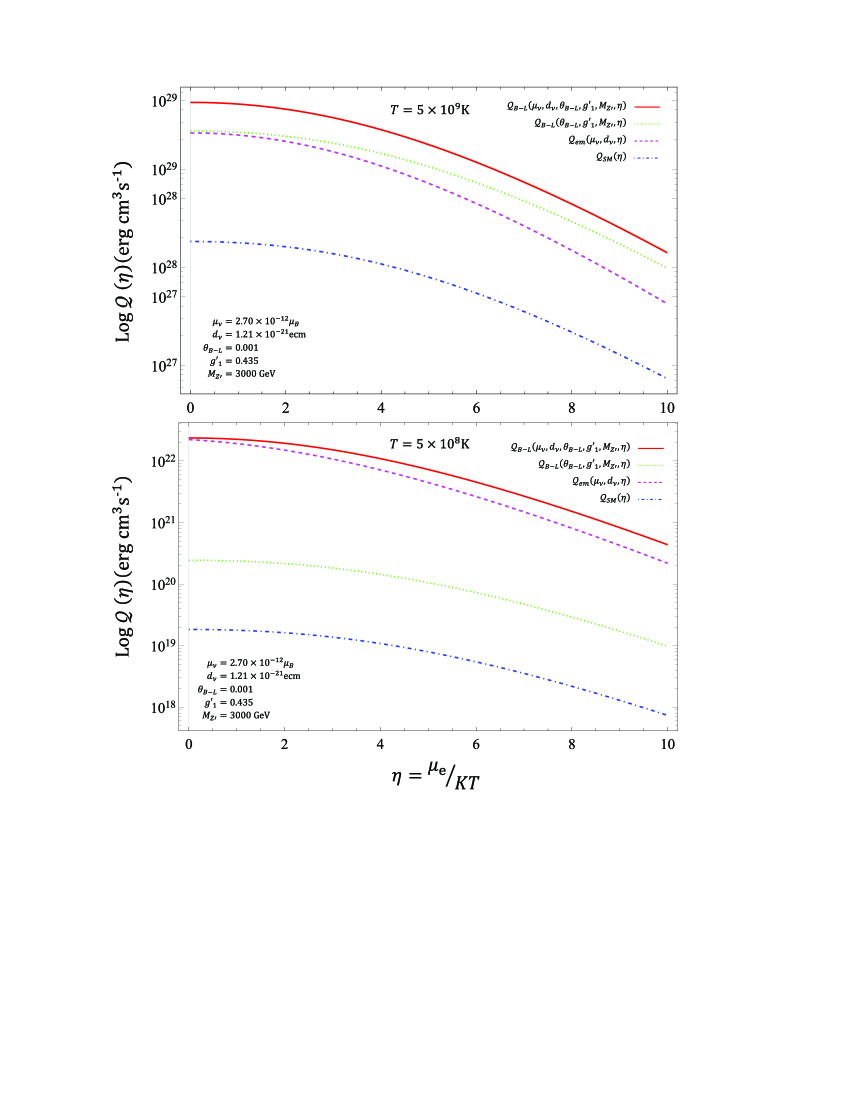
Figure 2: The stellar energy loss rates as a function of the degeneration parameter $\eta$ for stellar temperature of $5\times 10^{8}$K and $5\times 10^{9}$K. The solid line is for $\mathcal{Q}_{B-L}\left(\mu_{\nu},d_{\nu},\theta_{B-L},g^{\prime}_{1},M_{Z^{\prime}},\eta\right)$, the tiny dashes line is for $\mathcal{Q}_{B-L}\left(\theta_{B-L},g^{\prime}_{1},M_{Z^{\prime}},\eta\right)$, the large dashes line is for $\mathcal{Q}_{em}\left(\mu_{\nu},d_{\nu},\eta\right)$ and the dot-dashes line is for $\mathcal{Q}_{SM}\left(\eta\right)$.

The stellar energy loss rates for the process of pair-annihilation $e^{+}e^{-}\to(\gamma,Z,Z^{\prime})\to\nu\bar{\nu}$ as a function of the degeneration parameter $\eta$ are presented in Fig. 2, corresponding to input parameters $g^{\prime}_{1}=0.435$, $M_{Z^{\prime}}=3000$ GeV, $\theta_{B-L}=10^{-3}$, $\mu_{\nu}=2.70\times 10^{-12}\mu_{B}$ Kuznetsov-MM and $d_{\nu}=1.21\times 10^{-21}ecm$ bugarin2017 . In this figure we consider the following scenarios, $\mathcal{Q}_{B-L}\left(\mu_{\nu},d_{\nu},\theta_{B-L},g^{\prime}_{1},M_{Z^{\prime}},\eta\right)$ the stellar energy loss rates as a function of the dipole moments of the neutrino, the parameters of the B-L model and the degeneration parameter $\eta$, that is to say the $\mathcal{Q}_{B-L}$ correspond to the B-L model with electromagnetic properties. Another case corresponds to $\mathcal{Q}_{B-L}\left(\theta_{B-L},g^{\prime}_{1},M_{Z^{\prime}},\eta\right)$ the stellar energy loss rates as a function of the parameters of the B-L model and the degeneration parameter $\eta$, that is the $\mathcal{Q}_{B-L}$ correspond to the $U(1)_{B-L}$ model and without electromagnetic properties of the neutrino. The third case correspond to $\mathcal{Q}_{em}\left(\mu_{\nu},d_{\nu},\eta\right)$ the stellar energy loss rates as a function of the dipole moments of the neutrino and the degeneration parameter $\eta$, this case refers to the minimal extension of the SM with electromagnetic properties of the neutrino. Finally, the $\mathcal{Q}_{SM}\left(\eta\right)$ corresponds to the case of SM. These results show that both the dipole moments and the parameters of the B-L model have an important effect on the stellar energy loss rates. For instance, the difference between the cases with and without electromagnetic properties for the B-L model is 2 orders of magnitude. For the cases of the SM and the minimally extended SM with electromagnetic properties the difference is up to 3 orders of magnitude. Fig. 2 reveals that emissivity becomes larger with the contribution of the AMM and of the EDM of the neutrino, as well as with the parameters of the B-L model.

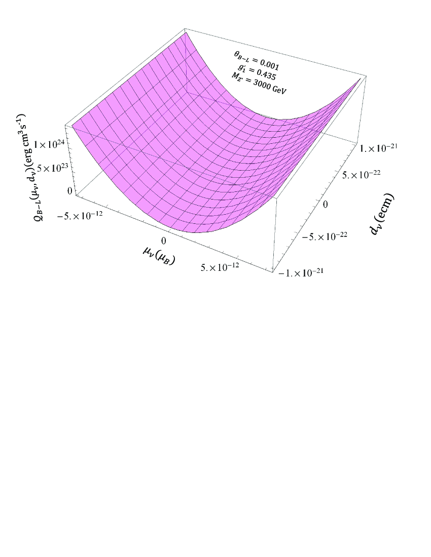
Figure 3: The stellar energy loss rates as a function of the AMM and the EDM $(\mu_{\nu},d_{\nu})$ for $\eta=2$.

Variation of ${\cal Q}_{B-L}\left(\mu_{\nu},d_{\nu},\eta\right)$ as a function of $\mu_{\nu}$ and $d_{\nu}$ with $g^{\prime}_{1}=0.435$, $M_{Z^{\prime}}=3000$ GeV, $\theta_{B-L}=10^{-3}$ and degeneration parameter $\eta=2$, respectively, is shown in Fig. 3. This, clearly shows a strong dependence of ${\cal Q}_{B-L}\left(\mu_{\nu},d_{\nu},\eta\right)$ with respect to the AMM of the neutrino and it is almost independent of the EDM, in agreement with a previous analysis presented in Ref. kerimov1992 .

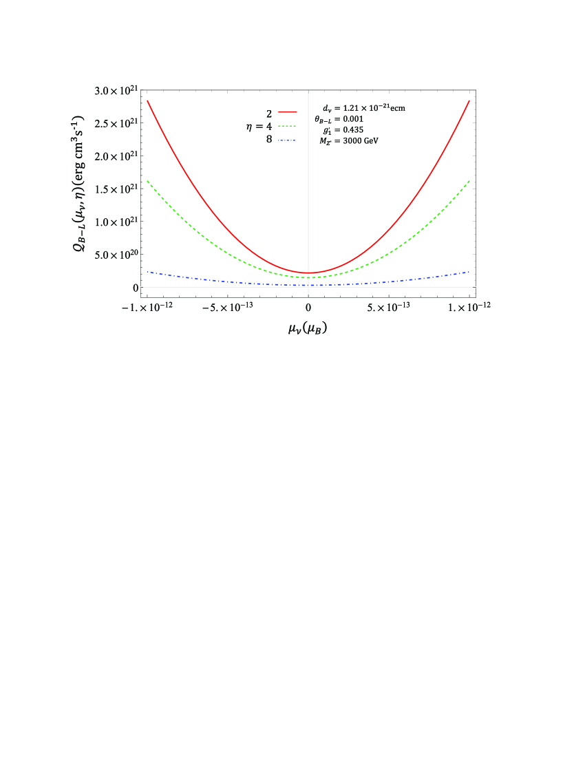
Figure 4: The stellar energy loss rate as a function of the AMM of the neutrino. The solid line is for $\eta=2$, the dashes line is for $\eta=4$ and the dot-dashes line is for $\eta=8$.

The dependence of ${\cal Q}\left(\mu_{\nu},\eta\right)$ with respect to $\mu_{\nu}$ is display in Fig. 4, with degeneration parameters $\eta=2,4,8$. From this figure we see that the stellar energy loss rates depend significantly on both, the AMM and the degeneration parameter $\eta$. The stellar energy loss rates also decreases as increasing $\eta$, which is due to the reduction in the number of positrons involved in the collisions.

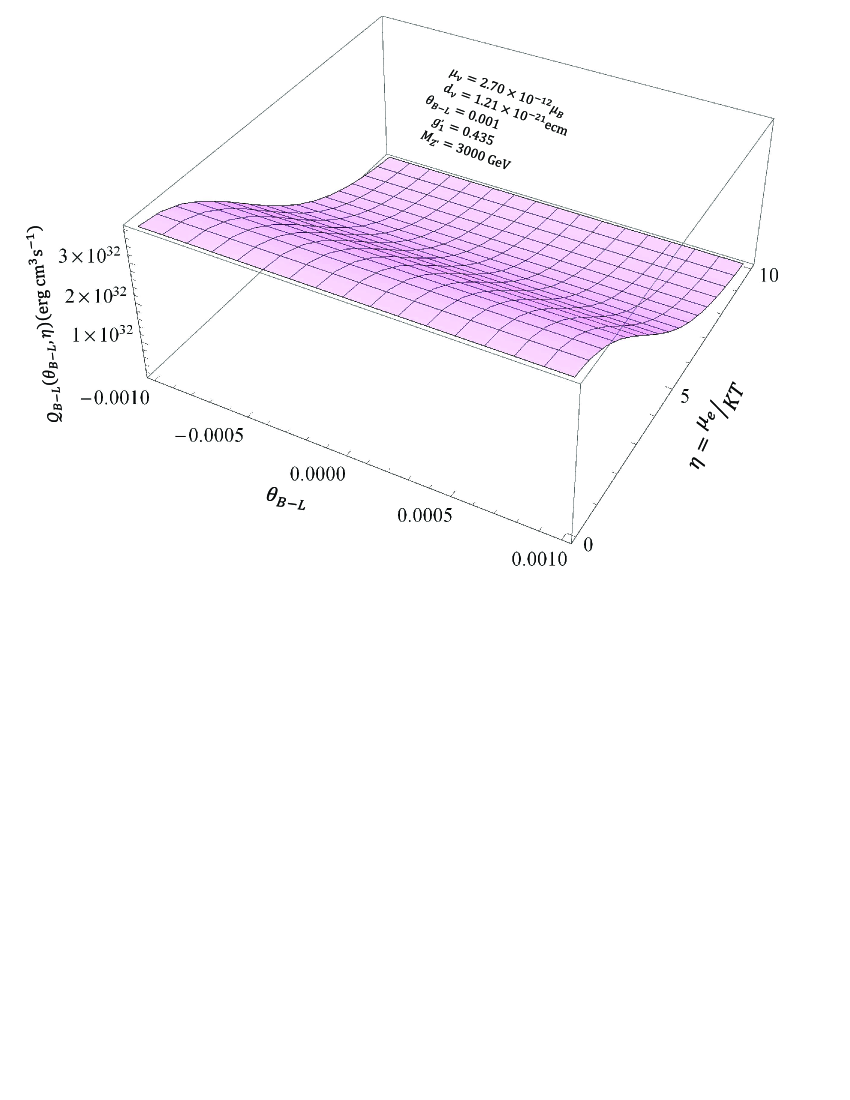
Figure 5: The stellar energy loss rates as a function of degeneration parameter and the mixing angle $(\eta,\theta_{B-L})$.

The dependence of ${\cal Q}\left(\theta_{B-L},\eta\right)$ on the pair of parameters $(\theta_{B-L},\eta)$ is shown in Fig. 5. The stellar energy loss rates decreases when $\eta$ increases. This behaviour is due to the reduction of the number of positrons available to cause the collision. Besides, the stellar energy loss rates keeps nearly constant for any value of the mixing angle $\theta_{B-L}$.

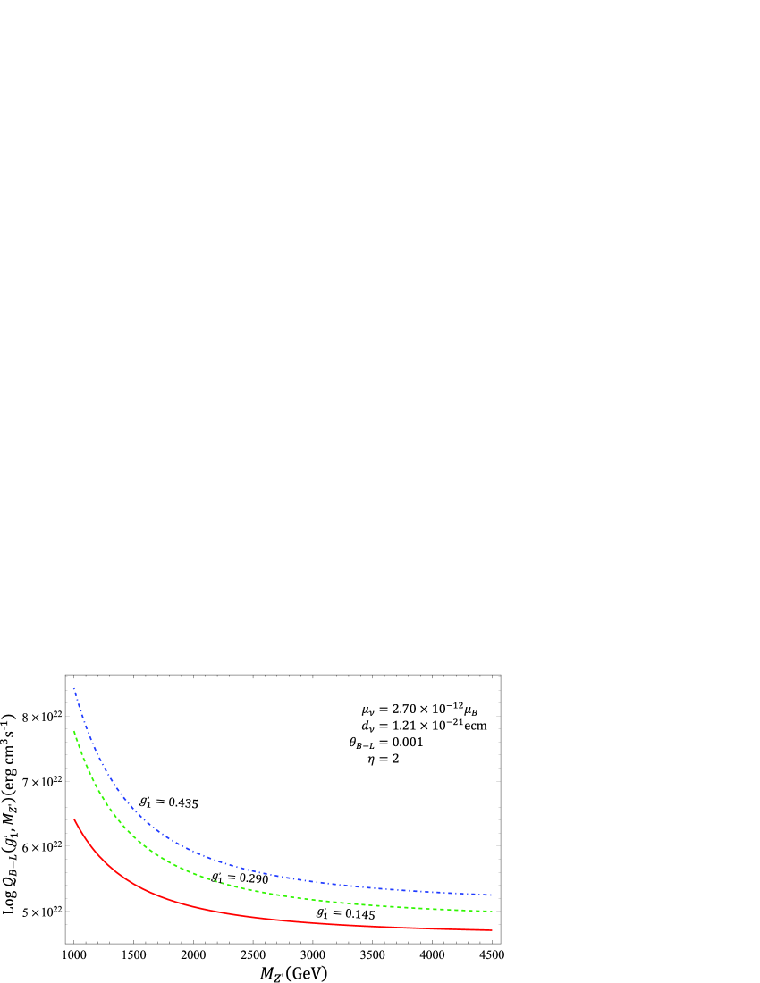
Figure 6: The stellar energy loss rates as a function of the mass of the new gauge boson $M_{Z^{\prime}}$. The solid line is for $g^{\prime}_{1}=0.145$, the dashes line is for $g^{\prime}_{1}=0.290$ and the dot-dashes line is for $g^{\prime}_{1}=0.435$.

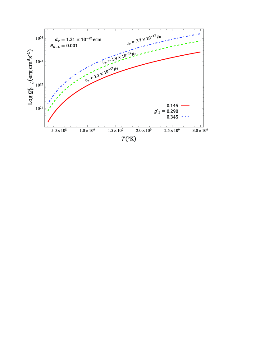
Figure 7: The stellar energy loss rates as a function of the stellar temperature $T$. The solid line is for $g^{\prime}_{1}=0.145$, the dashes line is for $g^{\prime}_{1}=0.290$ and the dot-dashes line is for $g^{\prime}_{1}=0.435$.

Fig. 6 shows the variation of the stellar energy loss rates as a function of the new gauge boson mass $M_{Z^{\prime}}$ from the $U(1)_{B-L}$ model with $g^{\prime}_{1}=0.145,0.290,0.435$. A dependance on both $M_{Z^{\prime}}$ and $g^{\prime}_{1}$ is observed for ${\cal Q}\left(M_{Z^{\prime}},g^{\prime}_{1},\eta\right)$. This result comes directly from the relation $M_{Z^{\prime}}=2v^{\prime}g^{\prime}_{1}$ khalil2008 ; emam2007 ; basso2009 . In Fig. 7, we show the stellar energy loss rates for the annihilation process $e^{+}e^{-}\rightarrow(\gamma,Z,Z^{\prime})\to\nu\bar{\nu}$ with contribution weak and electromagnetic. The high temperature enhancement of the electromagnetic annihilation channel discussed in section II is evident. For an AMM of $10^{-12}\mu_{B}$ and an EDM of $10^{-21}ecm$ the electromagnetic annihilation rates dominates over the rates for an AMM of $10^{-12}\mu_{B}$ and an EDM of $10^{-21}ecm$, respectively. Clearly magnetic and electric dipole moments of order minor that of $10^{-12}\mu_{B}$ and $10^{-21}ecm$ have less influence on the annihilation channel.

A simple comparison of the SM and the $U(1)_{B-L}$ model for pair production $e^{+}e^{-}\to(\gamma,Z,Z^{\prime})\to\nu\bar{\nu}$ is obtained using the full expressions of $\mathcal{Q}_{B-L}\left(\mu_{\nu},d_{\nu},\theta_{B-L},g^{\prime}_{1},M_{Z^{\prime}}\right)$ given by Eq. (18) and the corresponding of the SM which is obtained in the decoupling limit when $\theta_{B-L}=0$, $g^{\prime}_{1}=0$, $M_{Z^{\prime}}\to\infty$ and $\mu_{\nu}=d_{\nu}=0$.

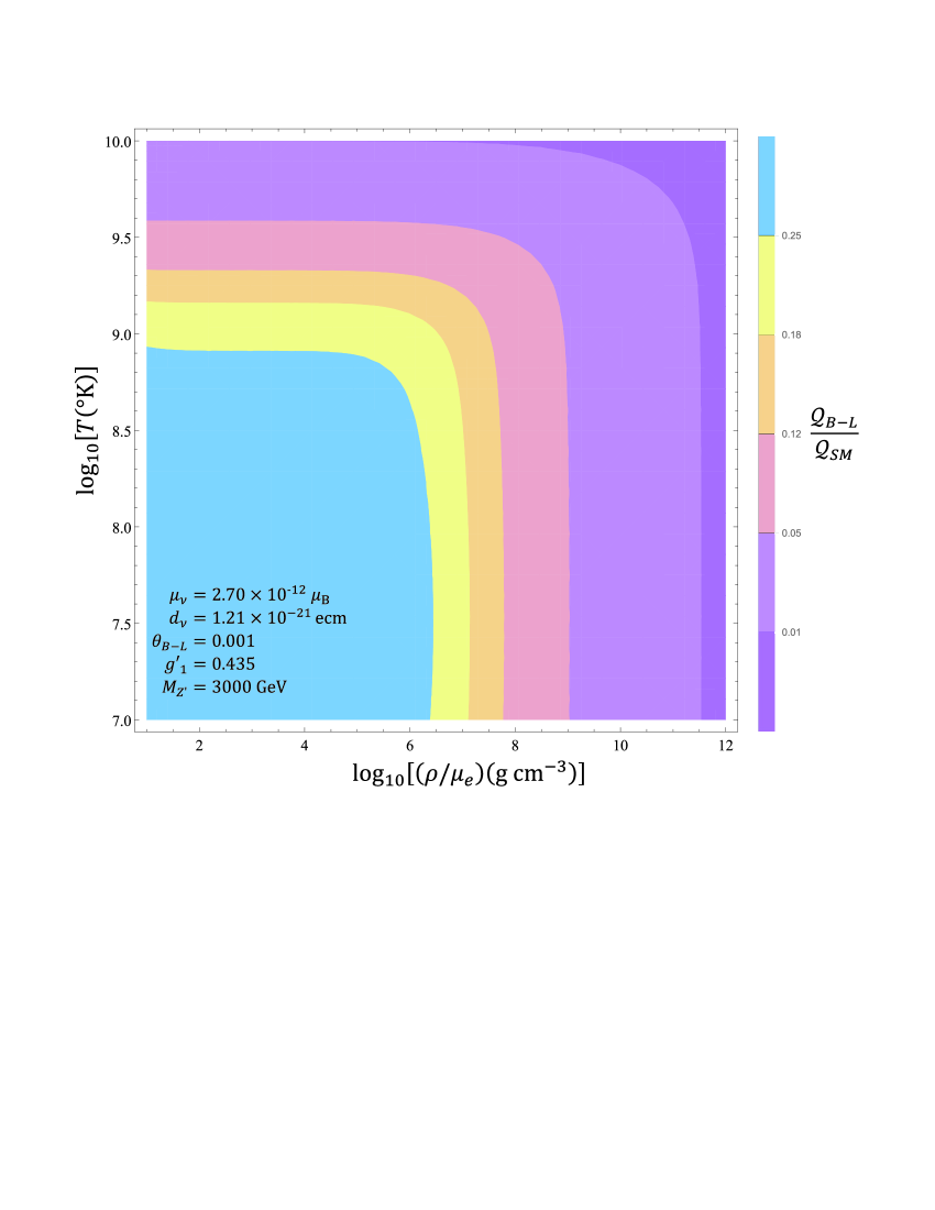
Figure 8: Contour plot of the ratio $\frac{\mathcal{Q}_{B-L}(\mu_{\nu},d_{\nu},\theta_{B-L},g^{\prime}_{1},M_{Z^{\prime}})}{\mathcal{Q}_{SM}}$ as a function of temperature $(T)$ and matter density $(\rho)$.

In this regard, Fig. 8 shows the contour plot of the ratio $\frac{\mathcal{Q}_{B-L}(\mu_{\nu},d_{\nu},\theta_{B-L},g^{\prime}_{1},M_{Z^{\prime}})}{\mathcal{Q}_{SM}}$ in the $(T,\rho/\mu_{e})$ parameter space, where the input parameters are $g^{\prime}_{1}=0.435$, $M_{Z^{\prime}}=3000$ GeV, $\theta_{B-L}=10^{-3}$, $\mu_{\nu}=2.70\times 10^{-12}\mu_{B}$ and $d_{\nu}=1.21\times 10^{-21}ecm$, respectively. This figure show the contours of the ratio $\mathcal{Q}_{B-L}\left(\mu_{\nu},d_{\nu},\theta_{B-L},g^{\prime}_{1},M_{Z^{\prime}}\right)/\mathcal{Q}_{SM}$ of nonstandard over standard energy loss via neutrino pair production as a function of temperature $(T)$ and matter density $(\rho)$ in the region of interest defined by $10^{1}\leq(\rho/\mu_{e})(gcm^{-3})\leq 10^{12}$ and $10^{7}\leq T(^{0}K)\leq 10^{10}$. The results show that indeed the $U(1)_{B-L}$ model loss does not exceeds $25\%$ of the SM one.

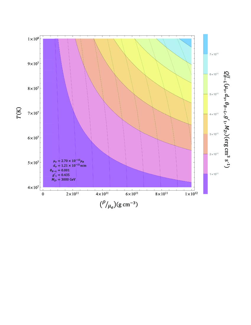
Figure 9: Contours in the plane $(T,\rho/\mu_{e})$ for the Region II. The AMM of the neutrino is fixed at $\mu_{\nu}=2.70\times 10^{-12}\mu_{B}$.

Starting from the expression for $\mathcal{Q}^{B-L}_{II}$ given by Eq. (24), we shows the contours plot in the $(T,\rho/\mu_{e})$ plane for different $\mathcal{Q}_{II}^{B-L}\left(\mu_{\nu},d_{\nu},\theta_{B-L},g^{\prime}_{1},M_{Z^{\prime}}\right)$, as shown in the color code for $\mathcal{Q}_{II}^{B-L}\left(\mu_{\nu},d_{\nu},\theta_{B-L},g^{\prime}_{1},M_{Z^{\prime}}\right)$, and the AMM of the neutrino is fixed at $\mu_{\nu}=2.70\times 10^{-12}\mu_{B}$. Our results are show in Fig. 9.

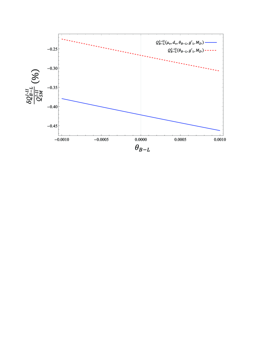
Figure 10: The relative correction $\dfrac{\delta\mathcal{Q}_{B-L}^{I-II}}{\mathcal{Q}_{SM}^{I-II}}$ as a function of the mixing angle $\theta_{B-L}$ with and without dependence of the AMM and the EDM $(\mu_{\nu},d_{\nu})$ for Regions I and II.

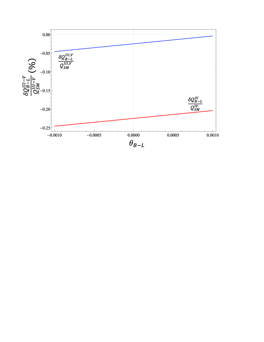
Figure 11: The relative correction $\dfrac{\mathcal{Q}_{B-L}^{III-V}\left(\mu_{\nu},d_{\nu},\theta_{B-L},g^{\prime}_{1},M_{Z^{\prime}},\eta\right)-\mathcal{Q}_{SM}^{III-V}\left(\eta\right)}{\mathcal{Q}_{SM}^{III-V}\left(\eta\right)}$ as a function of the mixing angle $\theta_{B-L}.$

To visualize and quantify the effects of the dipole moments $\mu_{\nu}$ and $d_{\nu}$ of the neutrino, as well as of the parameters $g^{\prime}_{1}$, $\theta_{B-L}$ and $M_{Z^{\prime}}$ of the $U(1)_{B-L}$ model on the stellar energy loss rates, we plot the relative correction $\frac{\delta{\cal Q}^{B-L}_{\nu\bar{\nu}}}{{\mathcal{Q}^{SM}_{\nu\bar{\nu}}}}$ for the regions I-II given by Eqs. (22) and (25) in Fig. 10. From this figure we observed that the relative correction $\frac{\delta{\cal Q}^{B-L}_{I-II}}{{\mathcal{Q}^{SM}}}$ is of the order of $22\%-46\%$ to the interval of $-10^{-3}\leq\theta_{B-L}\leq 10^{-3}$. While for the regions III-V, the relative correction $\frac{\delta{\cal Q}^{B-L}_{III-V}}{{\mathcal{Q}^{SM}}}$ given by Eqs. (28), (31) and (34) is of the order of $1\%-25\%$, as shown in Fig. 11.

To show the consistency of our model with the minimally extended standard model, as well as with the role in cosmology and astrophysics we estimated a sensitivity measure on the magnetic moment of the neutrino. Our obtained sensitivity measure is as follows. From Eqs. (21) or (24) corresponding to regions I and II where there is dependence on the AMM $(\mu_{\nu})$ and considering the ratio:

$$\frac{\mathcal{Q}^{B-L}_{I}}{\mathcal{Q}^{SM}_{I}} = \frac{M_{Z}^{4}\bigg{[}\Big{(}g_{1}^{[B-L]}+g_{2}^{[B-L]}\Big{)}+\frac{\sin^{4}{2\theta_{W}}\left(\mu_{\nu}^{2}+d_{\nu}^{2}\right)}{16\pi\alpha m_{e}^{2}}\bigg{]}}{\Big{(}g_{V}^{SM}\Big{)}^{2}},$$ (35)

it is possible to estimate sensitivity measure on the magnetic dipole moment of the neutrino which is competitive with other bounds reported in different astrophysical, cosmological and experimental approaches, as the ones mentioned in the Introduction. For instance, for the following values ​​of $\theta_{B-L}=10^{-3}$, $g^{\prime}_{1}=0.435$ and $M_{Z^{\prime}}=3000$ GeV we obtain the following sensitivity measure for the AMM:

$$|\mu_{\nu}|\leq 2.020\times 10^{-12}\mu_{B}.$$ (36)

Our sensitivity measure for the AMM given by Eq. (36) is consistent with that obtained through the Supernova energy loss studies lead to an upper limit of $\mu_{\nu}\lesssim(1.1-2.7)\times 10^{-12}\mu_{B}$ Kuznetsov-MM . In addition of the limits reported through the cooling rates of red giants $\mu_{\nu}\lesssim 3\times 10^{-12}\mu_{B}$ Raffelt-MM , of the analysis of cooling rates of white dwarfs $\mu_{\nu}\lesssim 10^{-11}\mu_{B}$ Blinnikov-MM , etc..

We show that the stellar energy loss rates significantly depends on the effective magnetic moment of the neutrino, as well as on the parameters of the $U(1)_{B-L}$ model, that is the mass of the new gauge boson $M_{Z}^{\prime}$ , the mixing angle $\theta_{B-L}$ between $Z-Z^{\prime}$ and the coupling constant $g^{\prime}_{1}$. Furthermore, our analytical formulas for the stellar energy loss rates in the B-L model approach are novel and are more general than the corresponding ones for the SM.

In the B-L model approach we estimated a sensitivity measure on the neutrino magnetic moment which is competitive with those obtained from astrophysical and experimental approach. See Eq. (36) about our sensitivity measure on the AMM.

For all the aforementioned, ${\cal Q}^{B-L}_{\nu\bar{\nu}}$ increases if one introduces new interactions that changes the neutrino annihilation cross-section. This is the case if the neutrino has a diagonal magnetic moment, because a magnetic moment would increase $\nu-\bar{\nu}$ annihilation (creation) into (by) $e^{\pm}$, keeping the neutrinos in equilibrium below the canonical (including only weak processes) neutrino decoupling temperature. In addition, as neutrino mass is sufficiently small, that is $m_{\nu}\ll m_{e}$ and remains coupled to electrons while the electrons annihilate, the neutrino number density will be increased because part of the electrons entropy will be shared with the neutrinos.

Until now, SN 1987A is the only supernova from which neutrinos have been detected. However, new generations of detectors of neutrinos will increase the capability detection of the order of ten thousand neutrinos from Via Lactea supernovas up to one more order of magnitude. As we just did, it will be possible to relate our results with data from observations or measurements such as supernova energy loss, cooling rates of red giants, cooling rates of white dwarfs, Borexino Experiment, TEXONO Collaboration, etc. through the neutrino magnetic moment.

IV Conclusions

We have developed and presented exact analytical formulas to assess the stellar energy loss rates involved in the process of emission of neutrinos driven by the channel $e^{+}e^{-}\to(\gamma,Z,Z^{\prime})\to\nu\bar{\nu}$. Thus, the stellar energy lost rates must be assessed completely with (18). The validity of such an equation extends to the cases whether or not electrons are degenerated or relativistic ones, a fact that is properly reflected in all the range of values considered for $\lambda$ and $\eta$. A fiduciary result is that the stellar energy lost rates increase and are considerably dependent on the electromagnetic dipole moments of the Dirac neutrinos and of the $U(1)_{B-L}$ parameters. The comparison $\mathcal{Q}_{B-L}\left(\mu_{\nu},d_{\nu},\theta_{B-L},g^{\prime}_{1},M_{Z^{\prime}}\right)/\mathcal{Q}_{SM}$ in the region of interest for $T$ and $\rho/\mu_{e}$ show that the $U(1)_{B-L}$ model loss does not exceeds $25\%$ of the SM one. Also, we find that the sensitivity estimated on magnetic dipole moment of the neutrino is of the order of $|\mu_{\nu}|\leq 2.020\times 10^{-12}\mu_{B}$, and it is competitive with other limits reported in the literature Barbieri-MM ; Kuznetsov-MM ; Raffelt-MM ; Blinnikov-MM ; Borexino-MM ; Texono-MM . The relative correction of $\frac{\delta{\cal Q}^{B-L}_{\nu\bar{\nu}}}{\mathcal{Q}^{SM}_{\nu\bar{\nu}}}$, given by $\frac{\delta\mathcal{Q}^{B-L}_{I-II}}{{\mathcal{Q}^{SM}}}$ is of $22\%-46\%$ for the regions I-II. For regions III-V the relative correction is of the order of $1\%-25\%$. The comparison $\mathcal{Q}_{B-L}\left(\mu_{\nu},d_{\nu},\theta_{B-L},g^{\prime}_{1},M_{Z^{\prime}}\right)/\mathcal{Q}_{SM}$ in the region of interest for $T$ and $\rho/\mu_{e}$ show that the $U(1)_{B-L}$ model loss does not exceeds $25\%$ of the SM one.

With our results, the process of pair-annihilation $e^{+}e^{-}\rightarrow(\gamma,Z,Z^{\prime})\to\nu\bar{\nu}$, open a number of opportunities to further study the stellar energy loss rates combining both, the effects of the AMM and the EDM of the neutrino, and the $U(1)_{B-L}$ parameters, with the inclusion of other potentially important channnels such as $\gamma+e^{\pm}\rightarrow e^{\pm}\nu\bar{\nu}$ ($\nu$- photoproduction), $\gamma^{*}\rightarrow\nu\bar{\nu}$ (plasmon decay) and $e^{\pm}+Z\rightarrow e^{\pm}+Z\nu\bar{\nu}$ (bremsstrahlung on nuclei). These processes are the dominant cause of the stellar energy loss rates in different regions present within the density-temperature plane. These new calculations, could contribute to a better understanding of the neutrino physics, and of new physics BSM Gutierrez2019 .

Acknowledgments

A. G. R. and M. A. H. R. thank SNI and PROFEXCE (México).

Appendix A Lagrangian of the $U(1)_{B-L}$ model

For the Lagrangian of the $U(1)_{B-L}$ model, the terms for the interactions between neutral gauge bosons $Z,Z^{\prime}$ and a pair of fermions of the SM can be written as khalil2008 ; emam2007 ; bugarin2017 :

$${\cal L}_{NC}=\frac{-ig}{\cos\theta_{W}}\sum_{f}\bar{f}\gamma^{\mu}\frac{1}{2}(g^{f}_{V}-g^{f}_{A}\gamma^{5})fZ_{\mu}+\frac{-ig}{\cos\theta_{W}}\sum_{f}\bar{f}\gamma^{\mu}\frac{1}{2}(g^{\prime f}_{V}-g^{\prime f}_{A}\gamma^{5})fZ^{\prime}_{\mu}.$$ (37)

Thus, the expressions for the new couplings between the $Z,Z^{\prime}$ bosons and the SM fermions are presented in Table I. As usual, the SM couplings are recovered in the limit when $\theta_{B-L}=0$ and $g^{\prime}_{1}=0$,

Table 1: New couplings of the $Z,Z^{\prime}$ bosons with the SM fermions. $g=e/\sin\theta_{W}$ and $\theta_{B-L}$ is the $Z-Z^{\prime}$ mixing angle.

Particle	Couplings
$f\bar{f}Z$	$g^{f}_{V}=T^{f}_{3}\cos\theta_{B-L}-2Q_{f}\sin^{2}\theta_{W}\cos\theta_{B-L}+\frac{2{g\prime}_{1}}{g}\cos\theta_{W}\sin\theta_{B-L},$
	$g^{f}_{A}=T^{f}_{3}\cos\theta_{B-L}$
$f\bar{f}Z^{\prime}$	${g^{\prime}}^{f}_{V}=-T^{f}_{3}\sin\theta_{B-L}-2Q_{f}\sin^{2}\theta_{W}\sin\theta_{B-L}+\frac{2{g^{\prime}}_{1}}{g}\cos\theta_{W}\cos\theta_{B-L},$
	${g\prime}^{f}_{A}=-T^{f}_{3}\sin\theta_{B-L}$

Appendix B Couplings Constants

In Eq. (18) we have redefined the coupling constants of the $U\left(1\right)_{B-L}$ model as:

$$g_{1}^{[B-L]} =\Bigg{[}\dfrac{1}{M_{Z}^{4}}\Big{(}\left(g_{V}^{e}\right)^{2}+\left(g_{A}^{e}\right)^{2}\Big{)}\Big{(}\left(g_{V}^{\nu}\right)^{2}+\left(g_{A}^{\nu}\right)^{2}\Big{)}+\dfrac{1}{M_{Z^{\prime}}^{4}}\Big{(}\left(g_{V}^{\prime e}\right)^{2}+\left(g_{A}^{\prime e}\right)^{2}\Big{)}$$

$$\qquad\times\Big{(}\left(g_{V}^{\prime\nu}\right)^{2}+\left(g_{A}^{\prime\nu}\right)^{2}\Big{)}+\dfrac{2}{M_{Z}^{2}M_{Z^{\prime}}^{2}}\big{(}g_{V}^{e}g_{V}^{\prime e}+g_{A}^{e}g_{A}^{\prime e}\big{)}\big{(}g_{V}^{\nu}g_{V}^{\prime\nu}+g_{A}^{\nu}g_{A}^{\prime\nu}\big{)}\Bigg{]},$$ (38)

$$g_{2}^{[B-L]} =\Bigg{[}\dfrac{1}{M_{Z}^{4}}\Big{(}\left(g_{V}^{e}\right)^{2}-\left(g_{A}^{e}\right)^{2}\Big{)}\Big{(}\left(g_{V}^{\nu}\right)^{2}+\left(g_{A}^{\nu}\right)^{2}\Big{)}+\dfrac{1}{M_{Z^{\prime}}^{4}}\Big{(}\left(g_{V}^{\prime e}\right)^{2}-\left(g_{A}^{\prime e}\right)^{2}\Big{)}$$

$$\qquad\times\Big{(}\left(g_{V}^{\prime\nu}\right)^{2}+\left(g_{A}^{\prime\nu}\right)^{2}\Big{)}+\dfrac{2}{M_{Z}^{2}M_{Z^{\prime}}^{2}}\big{(}g_{V}^{e}g_{V}^{\prime e}-g_{A}^{e}g_{A}^{\prime e}\big{)}\big{(}g_{V}^{\nu}g_{V}^{\prime\nu}+g_{A}^{\nu}g_{A}^{\prime\nu}\big{)}\Bigg{]}.$$ (39)

References

• (1) C. D. Kilpatrick, T. Takaro, R. J. Foley, C. N. Leibler, Y. Pan, R.D. Campbell, W. V. Jacobson-Galan, H. A. Lewis, J. E. Lyke, C. E. Max, S. A. Medallon and A. Rest., Month. Not. R. Astron. Soc. 480, Vol. 2, 2072 (2018).
• (2) M. A. Hendry, S.J. Smartt, R. M. Crockett et al., Month. Not. R. Astron. Soc. 369, 1303 (2006).
• (3) S. J. Smartt, Ann. Rev. Astron. Astroph. 47, Vol. 1, 63 (2009).
• (4) G. Beaudet, V. Petrosian, and E. Salpeter, Astrophys. J. 150, 979 (1967).
• (5) D. A. Dicus, Phys. Rev. D 6, 941 (1972).
• (6) D. A. Dicus, E. W. Kolb, D. N. Schramm, and D. L. Tubbs, Neutrino pair bremsstrahlung including neutral current effects, Tech. Rep. (Texas Univ., Austin (USA). Center for Particle Theory, 1976).
• (7) S. Alam, J. Anand, S. Biswas, and A. Goyal, Phys. Rev. D 40, 2712 (1989).
• (8) D. A. Dicus and E. W. Kolb, Phys. Rev. D 15, 977 (1977).
• (9) S. W. Bruenn, Astrophys. J. S. 58, 771 (1985).
• (10) A. Gutiérrez-Rodríguez, E. Torres-Lomas and A. González-Sánchez, Int. J. Mod. Phys. A 25, 12 (2010).
• (11) M. A. Hernández-Ruíz, A. Gutiérrez-Rodríguez and A. González-Sánchez, Eur. Phys. J. A 53, 1 (2017).
• (12) J. Ellis and K. A. Olive, Nucl. Phys. B 223, 252 (1983).
• (13) M. Tanabashi et al., Phys. Rev. D 98, 030001 (2018).
• (14) M. Gerbino and M. Lattanzi, arXiv:1712.07109v1 [astro-ph].
• (15) G. G. Raffelt, Stars as laboratories for fundamental physics: The astrophysics of neutrinos, axions, and other weakly interacting particles (University of Chicago press, 1996).
• (16) A. Payez, C. Evoli, T. Fischer, M. Giannotti, A. Mirizzi, and A. Ringwald, Journal of Cosmology and Astroparticle Physics 2015, 006 (2015).
• (17) T. Fischer, S. Chakraborty, M. Giannotti, A. Mirizzi, A. Payez, and A. Ringwald, Phys. Rev. D 94, 085012 (2016).
• (18) K. Fujikawa and R. Shrock, Phys. Rev. Lett. 45, 963 (1980).
• (19) Robert E. Shrock, Nucl. Phys. B206, 359 (1982).
• (20) M. Fukugita and T. Yanagida, Physics of Neutrinos and Applications to Astrophysics, (Springer, Berlin, 2003).
• (21) A. Llamas-Bugarín, A. Gutiérrez-Rodríguez, and M. A. Hernández-Ruíz, Phys. Rev. D 95, 116008 (2017) and references therein.
• (22) R. N. Mohapatra and P. B. Pal, Massive Neutrinos in Physics and Astrophysics, World Scientific Lecture Notes in Physics, Vol. 72, (2004).
• (23) H. Ko, D. Jang, M. Kusakabe and M. Cheoun, arXiv:1910.04984v1 [hep-ph].
• (24) B. Kerimov, S. Zeinalov, V. Alizade, and A. Mourao, Phys. Lett. B 274, 477 (1992).
• (25) S. Blinnikov, Mon. Not. Roy. Astron. Soc. 266, 289 (1994).
• (26) G. G. Raffelt, Phys. Rep. 320, 319 (1999).
• (27) A. Heger, A. Friedland, M. Giannotti, and V. Cirigliano, Astrophys. J. 696, 608 (2009).
• (28) C. Giunti and A. Studenikin, Rev. Mod. Phys. 87, 531 (2015).
• (29) A. Cisneros, Astrophysics and Space Science 10, 87 (1971).
• (30) R. Barbieri and R. N. Mohapatra, Phys. Rev. Lett. 61, 27 (1988).
• (31) A. V. Kuznetsov, N. V. Mikheev and A. A. Okrugin, arXiv:0907.2905 [hep-ph].
• (32) G. G. Raffelt, Phys. Rept. 320, 319 (1999) and references therein.
• (33) S. I. Blinnikov, N. V. Dunina-Barkovskaya, Mon. Not. R. Astron. Soc. 266, 289 (1994).
• (34) C. Arpesella, et al., [Borexino Collaboration], Phys. Rev. Lett. 101, 091302 (2008).
• (35) M. Deniz et al. [TEXONO Collaboration], Phys. Rev. D81, 072001 (2010).
• (36) R. N. Mohapatra and R. E. Marshak, Phys. Rev. Lett. 44, 1316 (1980).
• (37) R. Marshak and R. N. Mohapatra, Phys. Lett. B 91, 222 (1980).
• (38) W. Buchmüller, C. Greub, and P. Minkowski, Phys. Lett. B 267, 395 (1991).
• (39) W. Emam and S. Khalil, Eur. Phys. J. C 52, 625 (2007).
• (40) S. Khalil, J. Phys. G: Nuclear and Particle Physics 35, 055001 (2008).
• (41) E. D. Carlson, Nucl. Phys. B 286, 378 (1987).
• (42) L. Basso, A. Belyaev, S. Moretti, and C. H. Shepherd-Themistocleous, Phys. Rev. D 80, 055030 (2009).
• (43) S. Singirala, R. Mohanta, S. Patra and S. Rao, arXiv:1710.05775v2 [hep-ph].
• (44) J. F. Nieves, Phys. Rev. D 26, 3152 (1982).
• (45) B. Kayser and A. S. Goldhaber, Phys. Rev. D 28, 2341 (1983).
• (46) P. Vogel and J. Engel, Phys. Rev. D 39, 3378 (1989).
• (47) A. Billur, M. Köksal, A. Gutiérrez-Rodríguez and M. Hernández-Ruíz, Phys. Rev. D 98, 095013 (2018).
• (48) D. Yakovlev, A. Kaminker, O. Y. Gnedin, and P. Haensel, Physics Reports 354, 1 (2001).
• (49) S. Esposito, G. Mangano, G. Miele, I. Picardi, and O. Pisanti, Mod. Phys. Lett. A 17, 491 (2002).
• (50) S. Esposito, G. Mangano, G. Miele, I. Picardi, and O. Pisanti, Nucl. Phys. B 658, 217 (2003).
• (51) C. Aydin, Il Nuovo Cimento A (1965-1970) 105, 843 (1992).
• (52) A. Llamas-Bugarín, A. Gutiérrez-Rodríguez, A. González-Sánchez and M. A. Hernández-Ruíz. In progress.
Refer to caption