Reinforcement Learning with Feedback Graphs

Abstract

We study episodic reinforcement learning in Markov decision processes when the agent receives additional feedback per step in the form of several transition observations. Such additional observations are available in a range of tasks through extended sensors or prior knowledge about the environment (e.g., when certain actions yield similar outcome). We formalize this setting using a feedback graph over state-action pairs and show that model-based algorithms can leverage the additional feedback for more sample-efficient learning. We give a regret bound that, ignoring logarithmic factors and lower-order terms, depends only on the size of the maximum acyclic subgraph of the feedback graph, in contrast with a polynomial dependency on the number of states and actions in the absence of a feedback graph. Finally, we highlight challenges when leveraging a small dominating set of the feedback graph as compared to the bandit setting and propose a new algorithm that can use knowledge of such a dominating set for more sample-efficient learning of a near-optimal policy.

1 Introduction

There have been many empirical successes of reinforcement learning (RL) in tasks where an abundance of samples is available [36, 39]. However, for many real-world applications the sample complexity of RL is still prohibitively high. It is therefore crucial to simplify the learning task by leveraging domain knowledge in these applications. A common approach is imitation learning where demonstrations from domain experts can greatly reduce the number of samples required to learn a good policy [38]. Unfortunately, in many challenging tasks such as drug discovery or tutoring system optimization, even experts may not know how to perform the task well. They can nonetheless give insights into the structure of the task, e.g., that certain actions yield similar behavior in certain states. These insights could in principle be baked into a function class for the model or value-function, but this is often non-trivial for experts and RL with complex function classes is still very challenging, both in theory and practice [21, 14, 17, 19].

A simpler, often more convenient approach to incorporating structure from domain knowledge is to provide additional observations to the algorithm. In supervised learning, this is referred to as data augmentation and best practice in areas like computer vision with tremendous performance gains [27, 42]. Recent empirical work [31, 26, 28] suggests that data augmentation is similarly beneficial in RL. However, to the best of our knowledge, little is theoretically known about the question:

How do side observations in the form of transition samples (e.g. through data augmentation) affect the sample-complexity of online RL?

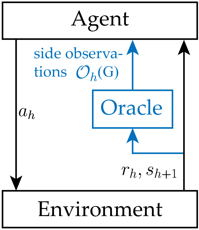
Figure 1: RL loop with side observations from a data augmentation oracle

In this paper, we take a first step toward answering this question and study RL in finite episodic Markov decision processes (MDPs) where, at each step, the agent receives some side information from an online data augmentation oracle, in addition to the reward and next state information $(r_{h},s_{h+1})$ directly supplied by the environment (Figure 1). This side information is a collection of observations, pairs of reward and next state, for some state-action pairs other than the one taken by the agent in that round. What can be observed is specified by a feedback graph [33] over state-action pairs: an edge in the feedback graph from state-action pair $(s,a)$ to state-action pair $(\bar{s},\bar{a})$ indicates that, when the agent takes action $a$ at state $s$, the oracle also provides the reward and next-state sample $(r^{\prime},s^{\prime})$ that it would have seen if it would have instead taken the action $\bar{a}$ at state $\bar{s}$. Specifically, at each time step, the agents not only gets to see the outcome of executing the current (s, a), but also an outcome of executing all the corresponding state-action pairs that have an edge from (s, a) in the feedback graph.

To illustrate this setting, consider a robot moving in a grid world. Through auxiliary sensors, it can sense positions in its line of sight. When the robot takes an action to move in a certain direction, it can also predict what would have happened for the same action in other positions in the line of sight. The oracle formalizes this ability and provides the RL algorithm with transition observations of (hypothetical) movements in the same direction from nearby states. Here, the feedback graph connects state-action pairs with matching states and actions in the line of sight (Figure 2).

For another illustrative example where feedback graphs occur naturally, consider a robot arm grasping different objects and putting them in bins. In this task, the specific shape of the object is relevant only when the robot hand is close to the object or has grasped it. In all other states, the actual shape is not significant and thus, the oracle can provide additional observations to the learning algorithm by substituting different object shapes in the state description of current transition. In this case, all such state-action pairs that are identical up to the object shape are connected in the feedback graph. This additional information can be easily modeled using a feedback graph but is much harder to incorporate in models such as factored MDPs [5] or linear MDPs [23]. RL with feedback graphs also generalizes previously studied RL settings, such as learning with aggregated state representations [16] and certain optimal stopping domains [18]. Furthermore, it can also be used to analyze RL with auxiliary tasks (see Section 5).

In this paper, we present an extensive study of RL with MDPs in the presence of side observations through feedback graphs. We prove in Section 4 that optimistic algorithms such as Euler or ORLC [41, 15] augmented with the side observations achieve significantly more favorable regret guarantees: the dominant terms of the bounds only depend on the mas-number $M$ of the feedback graph as opposed to an explicit dependence on $S$ and $A$, the number of states and actions of the MDP, which can be substantially larger than $M$ in many cases (See Table 1 for a summary of our results). We further give lower bounds which show that our regret bounds are in fact minimax-optimal, up to lower-order terms, in the case of symmetric feedback graphs (see Section 7).

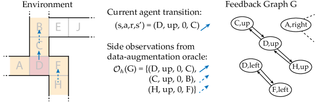
Figure 2: Example for RL with feedback graphs: Through additional sensors, the robot in state $D$ can also observe nearby states (yellow) and when taking the action up, the oracle provides the actual transition (solid arrow) as well as hypothetical transitions (dashed arrow) from nearby states. This is formalized by a feedback graph $G$ over state-action pairs shown on the right (snippet). Since $(D,up)$ has an edge to $(C,up)$ and $(G,up)$ in the feedback graph, the agent receives a (hypothetical) transition observation for both from the oracle.

While learning with feedback graphs has been widely studied in the multi-armed bandit setting [e.g. 33, 1, 9, 10, 2], the corresponding in the MDP setting is qualitatively different as the agent cannot readily access all vertices in the feedback graph (see section 6). A vertex $(s,a)$ of the feedback graph may be very informative but the agent does not know how to reach state $s$ yet. To formalize this, we prove through a statistical lower bound that leveraging a small dominating set to improve over the sample complexity of RL is fundamentally harder in MDPs than in multi-armed bandits. Finally, we propose a simple algorithm to addresses the additional challenges of leveraging a small dominating set in MDPs when learning an $\epsilon$-optimal policy and prove that its sample complexity scales with the size of the dominating set in the main $1/\epsilon^{2}$- term only.

2 Background and Notation

Episodic Tabular MDPs:

The agent interacts with an MDP in episodes indexed by $k$. Each episode is a sequence $(s_{k,1},a_{k,1},r_{k,1},\ldots,\allowbreak s_{k,H},a_{k,H},r_{k,H})$ of $H$ states $s_{k,h}\in\mathcal{S}$, actions $a_{k,h}\in\mathcal{A}$ and scalar rewards $r_{k,h}\in[0,1]$. The initial state $s_{k,1}$ can be chosen arbitrarily, possibly adversarially. Actions are taken as prescribed by the agent’s policy $\pi_{k}$ which are deterministic and time-dependent mappings from states to actions, i.e., $a_{k,h}=\pi_{k}(s_{k,h},h)$ for all time steps $h\in[H]:=\{1,2,\dots H\}$. The successor states and rewards are sampled from the MDP as $s_{k,h+1}\sim P(s_{k,h},a_{k,h})$ and $r_{k,h}\sim P_{R}(s_{k,h},a_{k,h})$.

State-action pairs $\mathcal{X}$:

We denote by $\mathcal{X}$ the space of all state-action pairs $(s,a)$ that the agent can encounter, i.e., visit $s$ and take $a$. The state space and action space are then defined as $\mathcal{S}=\{s\colon\exists a:~{}(s,a)\in\mathcal{X}\}$ and $\mathcal{A}=\{a\colon\exists s:~{}(s,a)\in\mathcal{X}\}$, respectively. This notation is more general than the typical definition of $\mathcal{S}$ and $\mathcal{A}$ and more convenient for our purposes. We restrict ourselves to tabular MDPs where $\mathcal{X}$ is finite. The agent only knows the horizon $H$ and $\mathcal{X}$, but has no access to the reward and transition distributions. For a pair $x\in\mathcal{X}$, we denote by $s(x)$ and $a(x)$ its state and action respectively.

Value Functions and Regret:

The Q-value of a policy is defined as the reward to go given the current state and action when the agent follows $\pi$ afterwards

$$Q^{\pi}_{h}(s,a):=\mathbb{E}\left[\sum_{t=h}^{H}r_{k,t}\Bigg{|}a_{k,h}=a,s_{k,h}=s,a_{k,h+1:H}\sim\pi\right],$$

and the state-values of $\pi$ are $V^{\pi}_{h}(s):=Q_{h}^{\pi}(s,\pi_{h}(s))$. The expected return of a policy in episode $k$ is simply the initial value $V^{\pi}_{1}(s_{k,1})$. Any policy that achieves optimal reward to go, i.e., $\pi(s,h)\in\mathop{\mathrm{argmax}}_{a}Q_{h}^{\pi}(s,a)$ is called optimal. We use superscript $\star$ to denote any optimal policy and its related quantities. The quality of an algorithm can be measured by its regret, the cumulative difference of achieved and optimal return, which after $T$ episodes is

$$R(T):=\sum_{k=1}^{T}(V^{\star}_{1}(s_{k,1})-V^{\pi_{k}}_{1}(s_{k,1})).$$

		Worst-Case Regret	Sample Complexity
without feedback graph	ORLC [11]	$\tilde{O}(\sqrt{{\color[rgb]{0.75,0,0}SA}H^{2}T}+{\color[rgb]{0.75,0,0}SA}\hat{S}H^{2})$	$\tilde{O}\left(\frac{{\color[rgb]{0.75,0,0}SA}H^{2}}{\epsilon^{2}}+\frac{{\color[rgb]{0.75,0,0}SA}\hat{S}H^{2}}{\epsilon}\right)$
	Lower bounds [12, 37]	$\tilde{\Omega}(\sqrt{{\color[rgb]{0.75,0,0}SA}H^{2}T})$	$\tilde{\Omega}\left(\frac{{\color[rgb]{0.75,0,0}SA}H^{2}}{\epsilon^{2}}\right)$
with feedback graph	ORLC [Thm. 1, Cor. 1]	$\tilde{O}(\sqrt{{\color[rgb]{0.078125,0.46875,0.078125}{M}}H^{2}T}+{\color[rgb]{0.078125,0.46875,0.078125}{M}}\hat{S}H^{2})$	$\tilde{O}\left(\frac{{\color[rgb]{0.078125,0.46875,0.078125}{M}}H^{2}}{\epsilon^{2}}+\frac{{\color[rgb]{0.078125,0.46875,0.078125}{M}}\hat{S}H^{2}}{\epsilon}\right)$
	Algorithm 2 [Thm. 4]	at least $O(\sqrt{{\color[rgb]{0.078125,0.46875,0.078125}{\gamma}}T^{2/3}})$	$\tilde{O}\left(\frac{{\color[rgb]{0.078125,0.46875,0.078125}{\gamma}}H^{3}}{p_{0}\epsilon^{2}}+\frac{{\color[rgb]{0.078125,0.46875,0.078125}{\gamma}}\hat{S}H^{2}}{p_{0}\epsilon}+\frac{{\color[rgb]{0.078125,0.46875,0.078125}{M}}\hat{S}H^{2}}{p_{0}}\right)$
	Lower bounds [Thm. 5, Thm. 6]	$\tilde{\Omega}(\sqrt{{\color[rgb]{0.078125,0.46875,0.078125}{\alpha}}H^{2}T})$	$\tilde{\Omega}\left(\frac{{\color[rgb]{0.078125,0.46875,0.078125}{\gamma}}H^{2}}{p_{0}\epsilon^{2}}+\frac{{\color[rgb]{0.078125,0.46875,0.078125}{\alpha}}}{p_{0}}\wedge\frac{{\color[rgb]{0.078125,0.46875,0.078125}{\alpha}}H^{2}}{\epsilon^{2}}\right)$

Table 1: Comparison of our main results. $\alpha$, $\gamma$ and $M$ denote the independence number, domination number and mas-number of the feedback graph respectively, with $\gamma\leq\alpha\leq M\leq SA$.

3 Reinforcement Learning in MDPs with Feedback Graphs

In the typical RL setting, when the agent takes action $a_{h}$ at state $s_{h}$, it can only observe the reward $r_{h}$ and next-state $s_{h+1}$. Thus, it only observes the transition $(s_{h},a_{h},r_{h},s_{h+1})$. Here, we assume that the agent additionally receives some side observations from an oracle (Figure 1). We denote by $\mathcal{O}_{k,h}(G)\subseteq\mathcal{X}\times[0,1]\times\mathcal{S}$ the set of transition observations thereby available to the agent in episode $k$ and time $h$. $\mathcal{O}_{k,h}(G)$ thus consists of the tuples $(s,a,r,s^{\prime})$ with state $s$, action $a$, reward $r$ and next state $s^{\prime}$, including the current transition $(s_{k,h},a_{k,h},r_{k,h},s_{k,h+1})$. For notational convenience, we also sometimes write transition tuples in the form $(x,r,s^{\prime})$ where $x=(s,a)$ is the state-action pair.

As discussed in Section 1, the oracle information is typically based on prior knowledge about the environment and additional sensors. The goal of this paper is not to study how specific oracles work but rather how RL algorithms can benefit from side observations. To that end, we formalize the side observations available to the agent by a directed graph $G=(\mathcal{X},E)$ over state-action pairs called a feedback graph. An edge $x\overset{G}{\rightarrow}\bar{x}$ (short for $(x,\bar{x})\in E$) from $x\in\mathcal{X}$ to $\bar{x}\in\mathcal{X}$ indicates that, when the agent takes action $a(x)$ at state $s(x)$, it can observe a reward and next-state sample $(r^{\prime},s^{\prime})$ it would have received, had it taken action $a(\bar{x})$ at state $s(\bar{x})$. To simplify the discussion, self-loops will be implicit and not included in the feedback graph. Essentially, $G$ only stipulates which side observations are available in addition to the currently performed transition. See Figure 2 for a concrete example. Formally, the set of transition observations received by the agent when it takes action $a_{h}$ at state $s_{h}$ is thus

$$\mathcal{O}_{h}(G)=\{((s_{h},a_{h}),r_{h},s_{h+1})\}\cup\{(x,r^{\prime},s^{\prime})\colon(s_{h},a_{h})\overset{G}{\rightarrow}x\},$$ (1)

where each observation $(x,r,s^{\prime})$ contains an independent sample from the next state distribution $s^{\prime}\sim P(x)$ and reward distribution $r\sim P_{R}(x)$ given all previous observations. Note that we allow simultaneous transition observations to be dependent.

Important Graph Properties:

The analysis of regret and sample-complexity in this setting makes use of following properties of the feedback graph:

• Mas-number $\bm{M}$: A set of vertices $\mathcal{V}\subseteq\mathcal{X}$ form an acyclic subgraph if the subgraph $(\mathcal{V},\{(v,w)\subseteq\mathcal{V}\times\mathcal{V}\colon v\overset{G}{\rightarrow}w\})$ of $G$ restricted to $\mathcal{V}$ is loop-free. We call the size of the maximum acyclic subgraph the mas-number $M$ of $G$.

• Independence number $\bm{\alpha}$: A set of vertices $\mathcal{V}\subseteq\mathcal{X}$ is an independent set if there is no edge between any two nodes of that set: $\forall v,w\in\mathcal{V}\colon v\,\not\overset{G}{\rightarrow}w$. The size of the largest independent set is called the independence number $\alpha$ of $G$.

• Domination number $\bm{\gamma}$: A set of vertices $\mathcal{V}\subset\mathcal{X}$ form a dominating set if there is an edge from a vertex in $\mathcal{V}$ to any vertex in $G$: $\forall x\in\mathcal{X}\;\exists v\in\mathcal{V}\colon v\overset{G}{\rightarrow}x$. The size of the smallest dominating set is called the domination number $\gamma$.

For any directed graph $G$,

$$\gamma\leq\alpha\leq M\leq|\mathcal{X}|,$$

where all the above inequalities can be a factor of $\Theta(|\mathcal{X}|)$ apart in the worst case. Independence- and mas-number coincide, $\alpha=M$, for symmetric (or undirected) graphs where for every edge there is an edge pointing backward. We defer to Appendix A a more extensive discussion with examples of how the above graph properties can differ from each other. Here, we only give two relevant examples:

1. State aggregation [16] can be considered a special case of learning with feedback graphs where the feedback graph consists of disjoint cliques, each consisting of the state-action pairs whose state belongs to a an aggregated state. Here $M=\alpha=\gamma=AB$ where $B$ is the number of aggregated states and $A=|\mathcal{A}|$.

2. Learning with auxiliary tasks where the agent aims to optimize several auxiliary reward functions can also be modeled as RL with a feedback graph where the MDP state space is augmented with a task identifier. See Section 5 for an extended discussion.

4 Graph Regret Bounds for Model-Based RL

In this section, we show the benefits of a feedback graph in achieving more favorable learning guarantees. We focus on model-based algorithms that follow the optimism in the face of uncertainty principle, a popular paradigm that achieves the tightest known regret / PAC bounds for the tabular MDP setting. Specifically, we will analyze a version of the Euler or ORLC algorithm [15, 41] shown in Algorithm 1.

The algorithm proceeds in rounds, and maintains first and second moments of the immediate reward i.e. $\widehat{r}(x)$ and $\widehat{r^{2}}(x)$ respectively, transition frequencies $\widehat{P}(x)$ and the number of observations $n(x)$ for each state-action pair $x\in\mathcal{X}$ as statistics to form an estimate of the true model. At the start of every round, in line 1, we compute a new policy $\pi_{k}$ using OptimistPlan, a version of value iteration with reward bonuses. Next, we execute the policy $\pi_{k}$ for one episode and update the model statistics using the samples collected.

The main difference between Algorithm 1 and the Euler or ORLC algorithms without feedback graphs is in the way we update our model statistics. Specifically, our algorithm also includes the additional observations $\mathcal{O}_{h}(G)$ available along with the current transition (as stipulated by the feedback graph $G$) to update the model statistics at the end of every round. This is highlighted in green in lines 1–1 of Algorithm 1.

Though being a straightforward extension of the previous algorithms, we show that Algorithm 1 can benefit from the feedback graph structure, and satisfies the following regret and certificates sizes (IPOC [15]) bound that only scales with the mas-number $M$ of the feedback graph $G$, and does not have any explicit dependence on size of the state or action space (in the dominant terms). Our main technical contribution is in the analysis, which we describe in the rest of this section.

input : failure tolerance $\delta\in(0,1]$, state-action space $\mathcal{X}$, episode length $H$;

input : maximum transition support $\widehat{S}\leq\|P(x)\|_{0}\leq S$;

1

2Initialize $n_{1}(x)\leftarrow 0,~{}\widehat{r}_{1}(x)\leftarrow 0,~{}\widehat{r^{2}}_{1}(x)\leftarrow 0,~{}\widehat{P}_{1}(x)\leftarrow e_{1}\in\{0,1\}^{S}$ for all $x\in\mathcal{X}$;

3 for episode $k=1,2,3,\dots$ do // Main Loop

       $(\pi_{k},\widetilde{V}_{k,h},\underaccent{\sim}{V}_{k,h})\leftarrow$ OptimistPlan($n_{k},\widehat{r}_{k},\widehat{r^{2}}_{k},\widehat{P}_{k}$) ;

        // VI with reward bonuses, see appendix

4       Receive initial state $s_{k,1}$ ;

5       $(n_{k+1},\widehat{r}_{k+1},\widehat{r^{2}}_{k+1},\widehat{P}_{k+1})\leftarrow$SampleEpisode($\pi_{k},s_{k,1},n_{k},\widehat{r}_{k},\widehat{r^{2}}_{k},\widehat{P}_{k}$) ;

6      

7 end for

8

9function SampleEpisode ($\pi,s_{1},n,\widehat{r},\widehat{r^{2}},\widehat{P}$):

10       for $h=1,\dots H$ do

11             Take action $a_{h}=\pi(s_{h},h)$ and transition to $s_{h+1}$ with reward $r_{h}$;

             Receive transition observations $\mathcal{O}_{h}(G)$;

              // As stipulated by feedback graph $G$

12             for transition $(x,r,s^{\prime})\in\mathcal{O}_{h}(G)$  do // Update empirical model and number of observations

13                   $\begin{array}[]{ll}n(x)\leftarrow n(x)+1,&\widehat{P}(x)\leftarrow\frac{n(x)-1}{n(x)}\widehat{P}(x)+\frac{1}{n(x)}e_{s^{\prime}},\\ \widehat{r}(x)\leftarrow\frac{n(x)-1}{n(x)}\widehat{r}(x)+\frac{1}{n(x)}r,&\widehat{r^{2}}(x)\leftarrow\frac{n(x)-1}{n(x)}\widehat{r^{2}}(x)+\frac{1}{n(x)}r^{2},\end{array}$

14                         where $e_{s^{\prime}}\in\{0,1\}^{S}$ has $1$ on the $s^{\prime}$-th position;

15                  

16             end for

             return : $(n,\widehat{r},\widehat{r^{2}},\widehat{P})$

17            

18       end for

19      

20

Algorithm 1 Optimistic model-based RL algorithm

Theorem 1 (Cumulative IPOC and regret bound).

For any tabular episodic MDP with episode length $H$, state-action space $\mathcal{X}\subseteq\mathcal{S}\times\mathcal{A}$ and directed feedback graph $G$, Algorithm 1 satisfies with probability at least $1-\delta$ an IPOC bound for all number of episodes $T$ of

$$\widetilde{O}\left(\sqrt{MH^{2}T}+M\widehat{S}H^{2}\right),$$ (2)

where $M$ is the size of the maximum acyclic subgraph of $G$ and algorithm parameter $\widehat{S}\leq S$ is a bound on the number of possible successor states of each $x\in\mathcal{X}$.
Equation (2) bounds the cumulative certificate size $\sum_{k=1}^{T}(\widetilde{V}_{1}(s_{k,1})-\underaccent{\sim}{V}_{1}(s_{k,1}))$ and the regret $R(T)$.

The above regret bound replaces a factor of $SA$ in the regret bounds for RL without side observations [15, 41] with the mas-number $M$ (see also Table 1). This is a substantial improvement since, in many feedback graphs $SA$ may be very large while $M$ is a constant. The only remaining polynomial dependency on $\widehat{S}\leq S$ in the lower-order term is typical for model-based algorithms.

On the lower bound side, we show in Section 7 that the regret is at-least $\widetilde{\Omega}(\sqrt{\alpha H^{2}T})$, where $\alpha$ denotes the independence number of $G$. While $M$ and $\alpha$ can differ by as much as $|\mathcal{X}|-1$ for general graphs, they match for symmetric feedback graphs (i.e. $M=\alpha$). In that case, our regret bound in Theorem 1 is optimal up to constant terms and $\log$-factors, and Algorithm 1 cannot be improved further.

We now discuss how the analysis of Theorem 1 differs from existing ones, with the full proof deferred to Appendix C. Assuming that the value functions estimated in OptimistPlan are valid confidence bounds, that is, $\underaccent{\sim}{V}_{k,h}\leq V^{\pi}_{h}\leq V^{\star}_{h}\leq\widetilde{V}_{k,h}$ for all $k\in[T]$ and $h\in[H]$, we bound regret as their differences

$$R(T)\leq\sum_{k=1}^{T}\big{[}\widetilde{V}_{k,1}(s_{k,1})-\underaccent{\sim}{V}_{k,1}(s_{k,1})\big{]}\lesssim\sum_{k=1}^{T}\sum_{h=1}^{H}\sum_{\begin{subarray}{c}x\in\mathcal{X}\end{subarray}}w_{k,h}(x)\left[H\wedge\left[\frac{\sigma_{k,h}(x)}{\sqrt{n_{k}(x)}}+\frac{\widehat{S}H^{2}}{n_{k}(x)}\right]\right],$$ (3)

where $\lesssim$ and $\gtrsim$ ignore constants and $\log$-terms and where $\wedge$ denotes the minimum operator. The second step is a bound on the value estimate differences derived through a standard recursive argument. Here, $w_{k,h}(x)=\mathbb{P}\big{(}(s_{k,h},a_{k,h})=x\mid\pi_{k},s_{k,1}\big{)}$ is the probability that policy $\pi_{k}$ visits $x$ in episode $k$ at time $h$. In essence, each such expected visit incurs regret $H$ or a term that decreases with the number of observations $n_{k}(x)$ for $x$ so far. In the expression above, $\sigma^{2}_{k,h}(x)=\operatorname{Var}_{r\sim P_{R}(x)}(r)+\operatorname{Var}_{s^{\prime}\sim P(x)}(V^{\pi_{k}}_{h+1}(s^{\prime}))$ is the variance of immediate rewards and the policy value with respect to one transition.

In the bandit case, one would now apply a concentration argument to turn $w_{k,h}(x)$ into actual visitation indicators but this would yield a loose regret bound of $\Omega(\sqrt{H^{3}T})$ here. Hence, techniques in the analysis of UCB in bandits with graph feedback [32] based on discrete pigeon-hole arguments cannot be applied here without incurring suboptimal regret in $H$. Instead, we apply a probabilistic argument to the number of observations $n_{k}(x)$. We show that, with high probability, $n_{k}(x)$ is not much smaller than the total visitation probability so far of all nodes $x^{\prime}\in\mathcal{N}_{G}(x):=\{x\}\cup\{x^{\prime}\in\mathcal{X}\colon x^{\prime}\overset{G}{\rightarrow}x\}$ that yield observations for $x$:

$$n_{k}(x)\gtrsim\sum_{i=1}^{k}\sum_{x^{\prime}\in\mathcal{N}_{G}(x)}w_{i}(x^{\prime}),\textrm{ with }w_{i}(x)=\sum_{h=1}^{H}w_{i,h}(x).$$

This only holds when $\sum_{i=1}^{k}\sum_{x^{\prime}\in\mathcal{N}_{G}(x)}w_{i}(x^{\prime})\gtrsim H$. Hence, we split the sum over $\mathcal{X}$ in (3) in $U_{k}=\left\{x\in\mathcal{X}\colon\sum_{i=1}^{k}\sum_{x^{\prime}\in\mathcal{N}_{G}(x)}w_{i}(x^{\prime})\gtrsim H\right\}$ and complement $U^{c}_{k}$. Ignoring fast decaying $1/n_{k}(x)$ terms, this yields

$$\eqref{eqn:basicbound1} \lesssim\sum_{k=1}^{T}\!\left[\sum_{x\in U_{k}^{c}}w_{k}(x)H+\!\!\sum_{x\in U_{k}}\sum_{h=1}^{H}w_{k,h}(x)\frac{\sigma_{k,h}(x)}{\sqrt{n_{k}(x)}}\right]$$

$$\lesssim\underbrace{\sum_{k=1}^{T}\sum_{x\in U_{k}^{c}}w_{k}(x)}_{({\text{A}})}H+\underbrace{\sqrt{\sum_{k=1}^{T}\sum_{x\in\mathcal{X}}\sum_{h=1}^{H}w_{k,h}(x)\sigma_{k,h}^{2}(x)}}_{({\text{B}})}~{}\cdot\underbrace{\sqrt{\sum_{k=1}^{T}\sum_{x\in U_{k}}\frac{w_{k}(x)}{\sum_{i=1}^{k}\sum_{x^{\prime}\in\mathcal{N}_{G}(x)}w_{i}(x^{\prime})}}}_{({\text{C}})},$$

where the second step uses the Cauchy-Schwarz inequality. The law of total variance for MDPs [3] implies that $({\text{B}})\lesssim H\sqrt{T}$. It then remains to bound $({\text{A}})$ and $({\text{C}})$, which is the main technical innovation in our proof. Observe that both $({\text{A}})$ and $({\text{C}})$ are sequences of functions that map each node $x$ to a real value $w_{k}(x)$. While $({\text{A}})$ is a thresholded sequence that effectively stops once a node has accumulated enough weight from the in-neighbors, $({\text{C}})$ is a self-normalized sequence. We derive the following two novel results to control each term. We believe these could be of general interest.

Lemma 2 (Bound on self-normalizing real-valued graph sequences).

Let $G=(\mathcal{X},\mathcal{E})$ be a directed graph with the finite vertex set $\mathcal{X}$ and mas-number $M$, and let $(w_{k})_{k\in[T]}$ be a sequence of weights $w_{k}:\mathcal{X}\rightarrow\mathbb{R}^{+}$ such that for all $k$, $\sum_{x\in\mathcal{X}}w_{k}(x)\leq w_{\max}$. Then, for any $w_{\min}>0$,

$$\sum_{k=1}^{T}\sum_{x\in\mathcal{X}}\frac{{\bf 1}\{w_{k}(x)\geq w_{\min}\}w_{k}(x)}{\sum_{i=1}^{k}\sum_{x^{\prime}\in\mathcal{N}_{G}(x)}w_{i}(x^{\prime})}\leq 2M\ln\left(eT\cdot\frac{w_{\max}}{w_{\min}}\right),$$ (4)

where $\mathcal{N}_{G}(x)=\{x\}\cup\{y\in\mathcal{X}~{}|~{}y\overset{G}{\rightarrow}x\}$ denotes the set of all vertices that have an edge to $x$ in $G$ and $x$ itself.

Lemma 3.

Let $G=(\mathcal{X},\mathcal{E})$ be a directed graph with vertex set $\mathcal{X}$ and let $w_{k}$ be a sequence of weights $w_{k}\colon\mathcal{X}\rightarrow\mathbb{R}^{+}$. Then, for any threshold $C\geq 0$,

$$\sum_{x\in\mathcal{X}}\sum_{k=1}^{\infty}w_{k}(x)\cdot{\bf 1}\left\{\sum_{i=1}^{k}\sum_{x^{\prime}\in\mathcal{N}_{G}(x)}w_{i}(x^{\prime})\leq C\right\}\leq MC$$ (5)

where $\mathcal{N}_{G}(x)$ is defined as in Lemma 2.

We apply Lemma 2 and Lemma 3 to get the bounds $({\text{A}})\lesssim MH$ and $({\text{C}})\lesssim\sqrt{M}$ respectively. Plugging these bounds back in (3) yields the desired regret bound. Note that both Lemma 2 and Lemma 3 above operate on a sequence of node weights as opposed to one set of node weights as in the technical results in the analyses of EXP-type algorithms [1]. The proof of Lemma 2 uses a potential function and a pigeon-hole argument. The proof for Lemma 3 relies on a series of careful reduction steps, first to integer sequences and then to certain binary sequences and finally a pigeon-hole argument. (full proofs are deferred to Appendix D).

5 Example Application of Feedback Graphs: Multi-Task RL

In this section, we show that various multi-task RL problems can be naturally modelled using feedback graphs and present an analysis of these problems. We consider the setting where there are $m$ tasks in an episodic tabular MDP. All tasks share the same dynamics $P$ but admit different immediate reward distributions $P_{R}^{(i)}$, $i\in[m]$. We assume the initial state is fixed, which generalizes without loss of generality to stochastic initial states. We further assume that the reward distributions of all but one task are known to the agent. Note that this assumption holds in most auxiliary task learning settings and does not trivialize the problem (see the next section for an example). The goal is to learn a policy that, given the task identity $i$, performs $\epsilon$-optimally. This is equivalent to learning an $\epsilon$-optimal policy for each task.

The naive solution to this problem consists of using $m$ instances of any existing PAC-RL algorithm to learn each task separately. Using Algorithm 1 as an example, this would require $\widetilde{O}\left(\frac{MH^{2}}{\epsilon^{2}}+\frac{\widehat{S}MH^{2}}{\epsilon}\right)$ episodes per task and in total

$$\widetilde{O}\left(\frac{m(1+\epsilon\widehat{S})MH^{2}}{\epsilon^{2}}\right)$$ (6)

episodes. When there is no additional feedback, the mas-number is simply the number of states and actions $M=SA$. If the number of tasks $m$ is large, this can be significantly more costly than learning a single task. We will now show that this dependency on $m$ can be removed when we learn the tasks jointly with the help of feedback graphs.

We can jointly learn the $m$ tasks by effectively running Algorithm 1 in an extended MDP $\bar{\mathcal{M}}$. In this extended MDP, the state is augmented with a task index, that is, $\bar{\mathcal{S}}=\mathcal{S}\times[m]$. In states with index $i$, the rewards are drawn from $P_{R}^{(i)}$ and the dynamics according to $P$ with successor states having the same task index. Formally, the dynamics $\bar{P}$ and immediate expected rewards $\bar{r}$ of the extended MDP is given by

$$\bar{P}((s^{\prime},j)|(s,i),a)={\bf 1}\{i=j\}P(s^{\prime}|s,a),\quad\text{and, }\quad\bar{r}((s,i),a)=r_{i}(s,a)$$ (7)

for all $s\in\mathcal{S}$, $a\in\mathcal{A}$, $i,j\in[m]$ where $r_{i}(s,a)=\mathbb{E}_{r\sim P_{R}^{(i)}(s,a)}[r]$ are the expected immediate rewards of task $i$. Essentially, the extended MDP consists of $m$ disjoint copies of the original MDP, each with the rewards of the respective task. Tabular RL without feedback graphs would also take as many episodes as Equation (6) to learn an $\epsilon$-optimal policy in this extended MDP for all tasks (e.g., when task index is drawn uniformly before each episode).

The key for joint learning is to define the feedback graph $\bar{G}$ so that it connects all copies of state-action pairs that are connected in the feedback graph $G$ of the original MDP. That is, for all $s,s^{\prime}\in\mathcal{S}$, $a,a^{\prime}\in\mathcal{A}$, $i,j\in[m]$,

$$((s,i),a)\overset{\bar{G}}{\rightarrow}~{} ((s^{\prime},j),a^{\prime})\Leftrightarrow(s,a)\overset{G}{\rightarrow}(s^{\prime},a^{\prime}).$$ (8)

Note that we can simulate an episode of $\bar{\mathcal{M}}$ by running the same policy in the original MDP because we assumed that the immediate rewards of all but one task are known. Therefore, to run Algorithm 1 in the extended MDP, it is only left to determine the task index $i_{k}$ of each episode $k$. To ensure learning all tasks equally fast and not wasting resources on a single task, it is sufficient to choose the task for which the algorithm would provide the largest certificate, i.e., $i_{k}\in\mathop{\mathrm{argmax}}_{i\in[m]}~{}\widetilde{V}_{k,1}((s_{k,1},i))-\underaccent{\sim}{V}_{k,1}((s_{k,1},i))$. This choice implies that if the certificate of the chosen task is smaller than $\epsilon$, then the same holds for all other tasks. Thus, by Theorem 1 above, Algorithm 1 must output a certificate with $\widetilde{V}_{k,1}((s_{k,1},i_{k}))-\underaccent{\sim}{V}_{k,1}((s_{k,1},i_{k}))\leq\epsilon$ after at most

$$\widetilde{O}\left(\frac{(1+\epsilon\widehat{S})MH^{2}}{\epsilon^{2}}\right)$$ (9)

episodes (see Corollary 1 in the appendix). Note that we used the mas-number $M$ and maximum number of successor states $\widehat{S}$ of the original MDP, as these quantities are identical in the extended MDP. Since $\epsilon\geq\widetilde{V}_{k,1}((s_{k,1},i_{k}))-\underaccent{\sim}{V}_{k,1}((s_{k,1},i_{k}))\geq\widetilde{V}_{k,1}((s_{k,1},j))-\underaccent{\sim}{V}_{k,1}((s_{k,1},j))\geq V^{\star}((s_{k,1},j))-V^{\pi_{k}}_{1}((s_{k,1},j))$ for all $j\in[m]$, the current policy $\pi_{k}$ is $\epsilon$-optimal for all tasks. Hence, by learning tasks jointly through feedback graphs, the total number of episodes needed to learn a good policy for all tasks does not grow with the number of tasks and we save a factor of $m$ compared to the naive approach without feedback graphs. This might seem to be too good to be true but it is possible because the rewards of all but one task are known and the dynamics is identical across tasks. Hence, additional tasks cannot add significant statistical complexity compared to the worst-case for a single task. While it may be possible to derive and analyze a specialized algorithm for this setting without feedback graphs, this would likely be much more tedious compared to this immediate approach leveraging feedback graphs.

6 Faster Policy Learning Using a Small Dominating Set

Algorithm 1 uses side observations efficiently (and close to optimally for symmetric feedback graphs), despite being agnostic to the feedback graph structure. Yet, sometimes, an alternative approach can be further beneficial. In some tasks, there are state-action pairs which are highly informative, that is, they have a large out-degree in the feedback graph, but yield low return. Consider for example a ladder in the middle of a maze. Going to this ladder and climbing it is time-consuming (low reward) but it reveals the entire structure of the maze, thereby making a subsequent escaping much easier. Explicitly exploiting such state-action pairs is typically not advantageous in regret terms (worst case $\Omega(T^{2/3})$) but that can be useful when the goal is to learn a good policy and when the return during learning is irrelevant. We therefore study the sample-complexity of RL in MDPs given a small dominating set $\mathcal{X}_{D}=\{X_{1},\dots,X_{\gamma}\}$ of the feedback graph.

We propose a simple algorithm that aims to explore the MDP by uniformly visiting state-action pairs in the dominating set. This works because the dominating set admits outgoing edges to every vertex, that is $\forall x\in\mathcal{X},\exists x^{\prime}\in\mathcal{X}_{D}\colon x^{\prime}\overset{G}{\rightarrow}x$. However, compared to bandits [1] with immediate access to all vertices, there are additional challenges for such an approach in MDPs:

1. Unknown policy for visiting the dominating: While we assume to know the identity of the state-action pairs in a dominating set, we do not know how to reach those pairs.

2. Low probability of reaching dominating set: Some or all nodes of the dominating set might be hard to reach under any policy.

The lower bound in Theorem 6 in the next section shows that these challenges are fundamental. To address them, Algorithm 2 proceeds in two stages. In the first stage (lines 2–2), we learn policies $\pi^{(i)}$ that visit each element $X_{i}\in\mathcal{X}_{D}$ in the dominating set with probability at least $\frac{p^{(i)}}{2}$. Here, $p^{(i)}=\max_{\pi}\mathbb{E}\left[\sum_{h=1}^{H}{\bf 1}\{(s_{h},a_{h})=X^{(i)}\}~{}|~{}\pi\right]$ is the highest expected number of visits to $X_{i}$ per episode possible.

The first phase leverages the construction for multi-task learning from Section 5. We define an extended MDP for a set of tasks $0,1,\dots,\gamma$. While task $0$ is to maximize the original reward, tasks $1,\dots,\gamma$ aim to maximize the number of visits to each element of the dominating set. We therefore define the rewards for each task of the extended MDP as

$$\bar{r}((s,0),a) =r(s,a) \bar{r}((s,k),a) ={\bf 1}\{(s,a)=X_{k}\},\quad\forall k\in[\gamma],s\in\mathcal{S},a\in\mathcal{A}.$$ (10)

The only difference with Section 5 is that we consider a subset of the tasks and stop playing a task once we have identified a sufficiently good policy for it. The stopping condition in Line 2 ensures that policy $\pi^{(i)}$ visits $X_{i}$ in expectation at least $\widehat{p}^{(i)}\geq\frac{p^{(i)}}{2}$ times. In the second phase of the algorithm (lines 2–2), each policy $\pi^{(i)}$ is played until there are enough samples per state-action pair to identify an $\epsilon$-optimal policy.

Theorem 4 (Sample-Complexity of Algorithm 2).

For any tabular episodic MDP with state-actions $\mathcal{X}$, horizon $H$, feedback graph with mas-number $M$ and given dominating set $\mathcal{X}_{D}$ with $|\mathcal{X}_{D}|=\gamma$ and accuracy parameter $\epsilon>0$, Algorithm 2 returns with probability at least $1-\delta$ an $\epsilon$-optimal policy after

$$O\left(\left(\frac{\gamma H^{3}}{p_{0}\epsilon^{2}}+\frac{\gamma\widehat{S}H^{3}}{p_{0}\epsilon}+\frac{M\widehat{S}H^{2}}{p_{0}}\right)\ln^{3}\frac{|\mathcal{X}|H}{\epsilon\delta}\right)$$ (11)

episodes. Here, $p_{0}=\min_{i\in[\gamma]}p^{(i)}$ is expected number of visits to the node in the dominating set that is hardest to reach.

The proof of Theorem 4 builds on the feedback graph techniques for Algorithm 1 and the arguments in Section 5. These arguments alone would yield an additional $\frac{MH^{2}}{p_{0}^{2}}$ term, but we show that is can be avoided through a more refined (and to the best of our knowledge, novel) argument in Appendix E.

The last term $\frac{M\widehat{S}H^{2}}{p_{0}}$ is spent in the first phase on learning how to reach the dominating set. The first two terms come from visiting the dominating set uniformly in the second phase. Comparing that to Corollary 1 for Algorithm 1, $M$ is replaced by $\frac{\gamma H}{p_{0}}$ in $\operatorname{poly}(\epsilon^{-1})$ terms. This can yield substantial savings when a small and easily accessible dominating set is known, e.g., when $\gamma\ll\frac{Mp_{0}}{H}$ and $\epsilon\ll p_{0}$. There is a gap between the bound above and the lower bound in Theorem 6, but one can show that a slightly specialized version of the algorithm reduces this gap to $H$ in the class of MDPs of the lower bound (by using that $p_{0}\leq 1,\hat{S}=2$ in this class, see Appendix E for details).

Extension to Unknown Dominating Sets: Since we pay only a logarithmic price for the number of tasks attempted to be learned in the first phase, we can modify the algorithm to attempt to learn policies to reach all $S$ states (and thus all $\mathcal{X}$) and stop the phase when an appropriate dominating set is found.

input : failure tolerance $\delta\in(0,1]$, desired accuracy $\epsilon>0$

input : dominating set $\mathcal{X}_{D}=\{X_{1},\dots,X_{\gamma}\}$, maximum transition support $\widehat{S}\leq\|P(x)\|_{0}\leq S$

1 Initialize $n(s,a)\leftarrow 0,~{}\widehat{r}(s,a)\leftarrow 0,~{}\widehat{r^{2}}(s,a)\leftarrow 0,~{}\widehat{P}(s,a)\leftarrow e_{1}$ for all $s\in\bar{\mathcal{S}}$ and $a\in\mathcal{A}$;

Set $\mathcal{I}\leftarrow\{1,\dots,\gamma\}$;

  // index set of active tasks

/* First phase: find policy to reach each vertex in given dominating set */

2 while $\mathcal{I}\neq\varnothing$ do

3      

      $\pi,\widetilde{V}_{h},\underaccent{\sim}{V}_{h}\leftarrow$ OptimistPlan($n,\widehat{r},\widehat{r^{2}},\widehat{P}$) ;

        // Alg. 3, with probability parameter $\delta/2$

4       $j\leftarrow\mathop{\mathrm{argmax}}_{i\in\mathcal{I}}\widetilde{V}_{1}((s_{1},i))-\underaccent{\sim}{V}_{1}((s_{1},i))$;

5       for $i\in\mathcal{I}$ do

6             if $\widetilde{V}_{1}((s_{1},i))\leq 2\underaccent{\sim}{V}_{1}((s_{1},i))$  then

7                  

                  $\pi^{(i)}((s,0),h)\leftarrow\pi((s,i),h)\qquad\forall s\in\mathcal{S},h\in[H]$;

                    // map policy to task 0

8                  

9                  $\widehat{p}^{(i)}\leftarrow\underaccent{\sim}{V}_{1}((s_{1},i))$;

10                   $\mathcal{I}\leftarrow\mathcal{I}\setminus\{i\}$;

11                  

12             end if

13            

14       end for

15      

      $n,\widehat{r},\widehat{r^{2}},\widehat{P}\leftarrow$ SampleEpisode($\pi,(s_{1},j),n,\widehat{r},\widehat{r^{2}},\widehat{P}$) ;

        // from Alg. 1, apply to extended MDP $\bar{\mathcal{M}}$

16      

17 end while

/* Second phase: play learned policies to uniformly sample from dominating set */

18

19while $\widetilde{V}_{1}((s_{1},0))-\underaccent{\sim}{V}_{1}((s_{1},0))>\epsilon$ do

20      

      $j\leftarrow(j\operatorname{mod}\gamma)+1$ ;

       // Choose policy in circular order

       $n,\widehat{r},\widehat{r^{2}},\widehat{P}\leftarrow$SampleEpisode($\pi^{(j)},(s_{1},0),n,\widehat{r},\widehat{r^{2}},\widehat{P}$) ;

        // from Alg. 1, apply to extended MDP $\bar{\mathcal{M}}\!\!\!$

       $\pi,\widetilde{V}_{h},\underaccent{\sim}{V}_{h}\leftarrow$ OptimistPlan($n,\widehat{r},\widehat{r^{2}},\widehat{P}$) ;

        // Alg. 3, with probability parameter $\delta/2$

21      

22 end while

$\hat{\pi}(s,h)\leftarrow\pi((s,0),h)\quad\forall s\in\mathcal{S},h\in[H]$;

 // map policy back to original MDP

return : $\hat{\pi}$

Algorithm 2 RL Using Dominating Set

7 Statistical Lower Bounds

RL in MDPs with feedback graphs is statistically easier due to side observations compared to RL without feedback graphs. Thus, existing lower bounds are not applicable. We now present a new lower-bound that shows that for any given feedback graph, the worst-case expected regret of any learning algorithm has to scale with the size of the largest independent set of at least half of the feedback graph.

Theorem 5.

Let $A,N,H,T\in\mathbb{N}$ and $G_{1},G_{2}$ be two graphs with $NA$ and $(N+1)A$ (disjoint) nodes each. If $H\geq 2+2\log_{A}N$, then there exists a class of episodic MDPs with $2N+1$ states, $A$ actions, horizon $H$ and feedback graph $G_{1}\cup G_{2}:=(V(G_{1})\cup V(G_{2}),E(G_{1})\cup E(G_{2}))$ such that the worst-case expected regret of any algorithm after $T$ episodes is at least $\frac{1}{46}\sqrt{\alpha H^{2}T}$ when $T\geq\alpha^{3}/\sqrt{2}$ and $\alpha\geq 2$ is the independence number of $G_{1}$.

The states in the class of MDPs in this lower bound form a deterministic tree with degree $A$ (bottom half of Figure 3). $G_{1}$ is the feedback graph for the state-action pairs at the leaves of this tree. They transition with slightly different probabilities to terminal states with high or low reward. Following Mannor and Shamir [33], we show that learning in such MDPs cannot be much easier than learning in $\alpha$-armed bandits where rewards are scaled by $H$. The same construction can be used to show a lower sample-complexity bound of order $\frac{\alpha H^{2}}{\epsilon^{2}}\ln\frac{1}{\delta}$ for learning $\epsilon$-optimal policies with probability at least $1-\delta$. This regret lower bound shows that, up to a scaling of rewards of order $H$, the statistical difficulty is comparable to the bandit case where the regret lower-bound is $\sqrt{\alpha T}$ [33].

The situation is different when we consider lower bounds in terms of domination number. Theorem 6 below proves that there is a fundamental difference between the two settings:

Theorem 6.

Let $\gamma\in\mathbb{N}$ and $p_{0}\in(0,1]$ and $H,S,A\in\mathbb{N}$ with $H\geq 2\log_{A}(S/4)$. There exists a family of MDPs with horizon $H$ and a feedback graph with a dominating set of size $\gamma$ and independence set of size $\alpha=\Theta(SA)$. The dominating set can be reached uniformly with probability $p_{0}$. Any algorithm that returns an $\epsilon$-optimal policy in this family with probability at least $1-\delta$ has to collect the following expected number of episodes in the worst case

$$\Omega\left(\frac{\alpha H^{2}}{\epsilon^{2}}\ln\frac{1}{\delta}\wedge\left(\frac{\gamma H^{2}}{p_{0}\epsilon^{2}}\ln\frac{1}{\delta}+\frac{\alpha}{p_{0}}\right)\right).$$ (12)

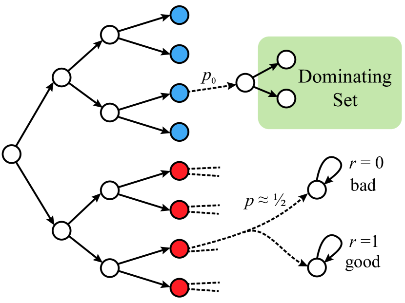
Figure 3: Difficult class of MDPs with a feedback graph and small dominating set. Omitted transitions point to the bad state.

This lower bound depends on the probability $p_{0}$ with which the dominating set can be reached and has a dependency $\frac{M}{p_{0}}\approx\frac{SA}{p_{0}}$ on the number of states and actions. In bandits, one can easily avoid the linear dependency on number of arms by uniformly playing all actions in the given dominating set $\tilde{\Theta}(\epsilon^{-2})$ times. We illustrate where the difficulty in MDPs comes from in Figure 6. States are arranged in a tree so that each state at the leafs can be reached by one action sequence.

The lower half of state-action pairs at the leafs (red) transition to good or bad terminal states with similar probability. This mimics a bandit with $\Theta(SA)$ arms. There are no side observations available except in state-action pairs of the dominating set (shaded area). Each of them can be reached by a specific action sequence but only with probability $p_{0}$, otherwise the agent ends up in the bad state.

To identify which arm is optimal in the lower bandit, the agent needs to observe $\Omega(H^{2}/\epsilon^{2})$ samples for each arm. It can either directly play all $\Theta(SA)$ arms or learn about them by visiting the dominating set uniformly. To visit the dominating set once takes $1/p_{0}$ attempts on average if the agent plays the right action sequence. However, the agent does not know which state-action at the leaf of the tree (blue states) can lead to the dominating set and therefore has to try each of the $\Theta(SA)$ options on average $1/p_{0}$ times to identify it.

8 Related Work

To the best of our knowledge, we are the first to study RL with feedback graphs in MDPs. In the bandit setting, there is a large body of works on feedback graphs going back to Mannor and Shamir [33]. In stochastic bandits, Caron et al. [7] provided the first regret bound for UCB in terms of clique covering number which was improved by Lykouris et al. [32] to mas-number. Both are gap-dependent bounds as is common in bandits. Simchowitz and Jamieson [40] recently proved the first gap-dependent bounds in MDPs for an algorithm similar to Algorithm 1 without graph feedback. To keep the analysis and discussion to the point, we here provided worst-case problem-independent bounds but we assume that a slight generalization of our technical results could be used to prove similar problem-dependent bounds.

While mas-number is the best-known dependency for UCB-style algorithms, Cohen et al. [8] achieved $\sqrt{\alpha T}$ regret with an elimination algorithm that uniformly visits independence sets in each round. Instead, Alon et al. [1] explicitly leveraged a dominating set for $\sqrt{\alpha T}$ regret. Finally, Buccapatnam et al. [6] also relies on the existence of a small dominating set to achieve problem-dependent regret scaling with $\gamma$. Unfortunately, all these techniques rely on immediate access to each node in the feedback graph which is unavailable in MDPs.

Albeit designed for different purposes, the first phase of Algorithm 2 is similar to a concurrently developed algorithm [24] for exploration in absence of rewards. But there is a key technical difference: Algorithm 2 learns how to reach each element of the dominating set jointly, while the approach by Jin et al. [24] learns how to reach each state-action pair separately. Following the discussion in Section 5, we hypothesize that by applying our technique to their setting, one could reduce the state-space dependency in the $\epsilon^{-1}$ term of their sample complexity bound from $S^{4}/\epsilon$ to $S^{3}/\epsilon$.

9 Conclusion

We studied the effect of data augmentation in the form of side observations governed by a feedback graph on the sample-complexity of RL. Our results show that optimistic model-based algorithms achieve minimax-optimal regret up to lower-order terms in symmetric feedback graphs by just incorporating all available observations. We also proved that exploiting the feedback graph structure by visiting highly informative state-action pairs (dominating set) is fundamentally more difficult in MDPs compared to the well-studied bandit setting. As RL with feedback graph in MDPs captures existing settings such as learning with state abstractions and learning with auxiliary tasks, our work paves the way for a more extensive study of this setting. Promising directions include a regret analysis for feedback graphs in combination with function approximation motivated by impressive empirical successes [31, 26, 28]. Another question of interest is an analysis of model-free methods [22] with graph feedback which likely requires a very different analysis, as existing proofs hinge on observations arriving in trajectories.

Acknowledgements.

The work of MM was partly supported by NSF CCF-1535987, NSF IIS-1618662, and a Google Research Award. KS would like to acknowledge NSF CAREER Award 1750575 and Sloan Research Fellowship. The work of YM was partly supported by a grant of the Israel Science Foundation (ISF).

Appendix A Discussion of Graph Properties

In this section, we provide an extended discussion of the relevant graph properties that govern learning efficiency of RL with feedback graphs. For convenience, we repeat the definitions of the properties from Section 3.

• Mas-number $\bm{M}$: A set of vertices $\mathcal{V}\subseteq\mathcal{X}$ form an acyclic subgraph if the subgraph $(\mathcal{V},\{(v,w)\subseteq\mathcal{V}\times\mathcal{V}\colon v\overset{G}{\rightarrow}w\})$ of $G$ restricted to $\mathcal{V}$ is loop-free. We call the size of the maximum acyclic subgraph the mas-number $M$ of $G$.

• Independence number $\bm{\alpha}$: A set of vertices $\mathcal{V}\subseteq\mathcal{X}$ is an independent set if there is no edge between any two nodes of that set: $\forall v,w\in\mathcal{V}\colon v\,\not\overset{G}{\rightarrow}w$. The size of the largest independent set is called the independence number $\alpha$ of $G$.

• Domination number $\bm{\gamma}$: A set of vertices $\mathcal{V}\subseteq\mathcal{X}$ form a dominating set if there is an edge from a vertex in $\mathcal{V}$ to any vertex in $G$: $\forall x\in\mathcal{X}\;\exists v\in\mathcal{V}\colon v\overset{G}{\rightarrow}x$. The size of the smallest dominating set is called the domination number $\gamma$.

• Clique covering number $\bm{\mathcal{C}}$: A set of vertices $\mathcal{V}\subseteq\mathcal{X}$ is a clique if there it is a fully-connected subgraph, i.e., for any $x,y\in\mathcal{V}\colon x\overset{G}{\rightarrow}y$. A set of such cliques $\{\mathcal{V}_{1},\dots\mathcal{V}_{n}\}$ is called a clique cover if every node is included in at least one of the cliques, i.e., $\mathcal{X}=\bigcup_{i=1}^{n}\mathcal{V}_{i}$. The size of the smallest clique cover is called the clique covering number $\mathcal{C}$.

In addition to the properties appearing our bounds, we here include the clique covering number $\mathcal{C}$ which has been used earlier analyses of UCB algorithms in bandits [7]. One can show that in any graph, the following relation holds

$$|\mathcal{X}|\geq\mathcal{C}\geq M\geq\alpha\geq\gamma.$$ (13)

For example, $\mathcal{C}\geq M$ follows from the fact that no two vertices that form a clique can be part of an acyclic subgraph and thus no acyclic subgraph can be larger than any clique cover. An important class of feedback graphs are symmetric feedback graphs where for each edge $x\overset{G}{\rightarrow}y$, there is a back edge $y\overset{G}{\rightarrow}x$. In fact, many analyses in the bandit settings assume undirected feedback graphs which is equivalent to symmetric directed graphs. For symmetric feedback graphs, the independence number and mas-number match, i.e.,

$$\alpha=M.$$ (14)

This is true because acyclic subgraphs of symmetric graphs cannot contain any edges, otherwise the back edge would immediately create a loop. Thus any acyclic subgraph is also an independent set and $M\geq\alpha$.

Examples:

We now discuss the value of the graph properties in feedback graphs by example (see Figure 4). The graph in Figure 4(a) consists of two disconnected cliques and thus the clique covering number and the domination number is $2$. While the total number of nodes can be much larger – 8 in this example – all graph properties equal the number of cliques in such a graph. In practice, feedback graphs that consists of disconnected cliques occur for example in state abstractions where all $(s,a)$ pairs with matching action and where the state belongs to the same abstract state form a clique. They are examples for a simple structure that can be easily exploited by RL with feedback graphs to substantially reduce the regret.

In the feedback graph in Figure 4(b), the vertices are ordered and every vertex is connected to every vertex to the left. This graph is acyclic and hence $M$ coincides with the number of vertices but the independence number is $1$ as the graph is a clique if we ignore the direction of edges (and thus each independence set can only contain a single node). A concrete example where feedback graphs can exhibit such structure is in tutoring systems where the actions represent the number of practice problems to present to a student in a certain lesson. The oracle can fill in the outcomes (how well the performed on each problem) for all actions that are would have given fewer problems than the chosen action.

Figure 4(c) shows a star-shaped feedback graph. Here, the center vertex reveals information about all other vertices and thus is a dominating set with size $\gamma=1$. At the same time, the largest independence set are the tips of the star which is much larger. This is an example where approaches such as Algorithm 2 that leverage a dominating set can learn a good policy with much fewer samples as compared to others that only rely independence sets.

The examples in Figure 4(a)–4(c) exhibit structured graphs, but it is important to realize that our results do not rely a specific structure. They can work with any feedback graph and we expect that feedback graphs in practice are not necessarily structured. Figure 4(d) shows a generic graph where all relevant graph properties are distinct which highlights that even in seemingly unstructured graphs, it is important which graph property governs the learning speed of RL algorithms.

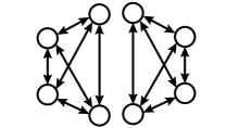
(a) $SA=8$
     $\mathcal{C}=M=\alpha=\gamma=2$

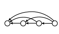
(b) $SA=\mathcal{C}=M=4$
     $\alpha=\gamma=1$

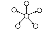
(c) $SA=6$
     $\mathcal{C}=M=\alpha=5$
     $\gamma=1$

(d) $SA=6$
     $\mathcal{C}=5,M=4$
     $\alpha=3,\gamma=2$

Figure 4: Examples of feedback graphs with different vertex numbers $SA$, mas-number $M$, independence number $\alpha$ and domination number $\gamma$.

Appendix B Additional Details on Model-Based RL with Feedback Graphs

Here, we provide additional details and extensions to Algorithm 1 in Section 4.

B.1 Optimistic Planning

Algorithm 3 presents the optimistic planning subroutine called by Algorithms 1 and 2. In this procedure, the maximum value is set as $V^{\max}_{h}=H-h+1$ for each time step $h$ and notation $\widehat{P}(x)f=\mathbb{E}_{s^{\prime}\sim P(x)}[f(x)]$ denotes the expectation with respect to the next state distribution of any function $f\colon\mathcal{S}\rightarrow\mathbb{R}$ on states.

The OptimistPlan procedure computes an optimistic estimate $\widetilde{Q}$ of the optimal Q-function $Q^{\star}$ by dynamic programming. The policy $\pi$ is chosen greedily with respect to this upper confidence bound $\widetilde{Q}$. In addition, a pessimistic estimate $\underaccent{\sim}{Q}$ of the Q-function of this policy $Q^{\pi}$ is computed (lower confidence bound) analogously to $\widetilde{Q}$. The two estimates only differ in the sign of the reward bonus $\psi_{h}$. Up to the specific form of the reward bonus $\psi_{h}(x)$, this procedure is identical to the policy computation in ORLC [15] and Euler [41].

1 function OptimistPlan ($n,\widehat{r},\widehat{r^{2}},\widehat{P}$):

2       Set $\widetilde{V}_{H+1}(s)\leftarrow 0;\quad\underaccent{\sim}{V}_{H+1}(s)\leftarrow 0\quad\forall s\in\mathcal{S}$;

3       for $h=H$ to $1$ and $s\in\mathcal{S}$ do // optimistic planning with upper and lower confidence bounds

4            

5            for $a\in\mathcal{A}$ do

6                   $x\leftarrow(s,a)$;

                   /* Compute reward bonus */

                   $\eta\leftarrow\sqrt{\widehat{r^{2}}(x)-\widehat{r}(x)^{2}}+\sqrt{\widehat{P}(x)(\widetilde{V}_{h+1}^{2})-(\widehat{P}(x)\widetilde{V}_{h+1})^{2}}$;

                   // Reward and next state variance

7                   $\psi_{h}(x)\leftarrow O\left(\frac{1}{H}\widehat{P}(x)[\widetilde{V}_{h+1}-\underaccent{\sim}{V}_{h+1}]+\sqrt{\frac{\eta}{n(x)}\ln\frac{|\mathcal{X}|H\ln n(x)}{\delta}}+\frac{\widehat{S}H^{2}}{n(x)}\ln\frac{|\mathcal{X}|H\ln n(x)}{\delta}\!\right)$ ;

                   /* Bellman backup of upper and lower confidence bounds */

                   $\widetilde{Q}_{h}(x)\leftarrow 0\vee\,\,(\widehat{r}(x)+\widehat{P}(x)\widetilde{V}_{h+1}+\psi_{h}(x))\,\,\wedge V^{\max}_{h}$ ;

                    // UCB of $Q^{\star}_{h}$

                   $\underaccent{\sim}{Q}_{h}(x)\leftarrow 0\vee\,\,(\widehat{r}(x)+\widehat{P}(x)\underaccent{\sim}{V}_{h+1}-\psi_{h}(x))\,\,\wedge V^{\max}_{h}$ ;

                    // LCB of $Q^{\pi}_{h}\geq 0$

8                  

9             end for

            /* Compute greedy policy of UCB */

10             $\pi(s,h)\leftarrow\mathop{\mathrm{argmax}}_{a}\widetilde{Q}_{h}(s,a)$;

11             $\widetilde{V}_{h}(s)\leftarrow\widetilde{Q}_{h}(s,\pi(h))$;        $\underaccent{\sim}{V}_{h}(s)\leftarrow\underaccent{\sim}{Q}_{h}(s,\pi(h))$;

12            

13       end for

      return : $\pi,\widetilde{V}_{h},\underaccent{\sim}{V}_{h}$

14      

15

Algorithm 3 Optimistic Planning Routine

B.2 Runtime Analysis

Just as in learning without graph feedback, the runtime of Algorithm 1 is $O(S\widehat{S}AH)$ per episode where $\widehat{S}$ is a bound on the maximum transition probability support ($S$ in the worst case). The only difference to RL without side observations is that there are additional updates to the empirical model. However, sampling an episode and updating the empirical model requires $O(HSA)$ computation as there are $H$ time steps and each can provide at most $|\mathcal{X}|\leq SA$ side observations. This is still dominated by the runtime of optimistic planning $O(S\widehat{S}AH)$. If the feedback graph is known ahead of time, one might be able to reduce the runtime, e.g., by maintaining only one model estimate for state-action pairs that form a clique in the feedback graph with no incoming edges. Then is suffices to only compute statistics of a single vertex per clique.

B.3 Sample Complexity

Since Algorithm 1 is a minor modification of ORLC, it follows the IPOC framework [15] for accountable reinforcement learning. As a result, we can build on the results for algorithms with cumulative IPOC bounds [11, Proposition 2] and show that our algorithm satisfies a sample-complexity guarantee:

Corollary 1 (PAC-style Bound).

For any episodic MDP with state-actions $\mathcal{X}$, horizon $H$ and feedback graph $G$, with probability at least $1-\delta$ for all $\epsilon>0$ jointly, Algorithm 1 can output a certificate with $\widetilde{V}_{k^{\prime},1}(s_{k^{\prime},1})-\underaccent{\sim}{V}_{k^{\prime},1}(s_{k^{\prime},1})$ for some episode $k^{\prime}$ within the first

$$k^{\prime}=O\left(\frac{MH^{2}}{\epsilon^{2}}\ln^{2}\frac{H|\mathcal{X}|}{\epsilon\delta}+\frac{M\hat{S}H^{2}}{\epsilon}\ln^{3}\frac{H|\mathcal{X}|}{\epsilon\delta}\right)$$ (15)

episodes. If the initial state is fixed, such a certificate identifies an $\epsilon$-optimal policy.

The proof of this corollary is available in Section C.6

B.4 Generalization to Stochastic Feedback Graphs

As presented in Section 3, we assumed so far that the feedback graph $G$ is fixed and identical in all episodes. We can generalize our results and consider stochastic feedback graphs where the existence of an edge in the feedback graph in each episode is drawn independently (from other episodes and edges). This means the oracle provides a side observation for another state-action pair only with a certain probability. We formalize this as the feedback graph $G_{k}$ in episode $k$ to be an independent sample from a fixed distribution where the probability an each edge is denoted as

$$q(x,x^{\prime}):=\mathbb{P}\left(x\overset{G_{k}}{\rightarrow}x^{\prime}\right).$$ (16)

This model generalizes the well-studied Erdős–Rényi model [e.g. 6] because different edges can have different probabilities. This can be used as a proxy for the strength of the user’s prior. One could for example choose the probability of states being connected to decreases with their distance. This would encode a belief that nearby states behave similarly.

Algorithm 1 can be directly applied to stochastic feedback graphs and as our analysis will show the bound in Theorem 1 still holds as long as the mas-number $M$ is replaced by

$$\bar{M}=\inf_{\epsilon\in(0,1]}\frac{M(G_{\geq\epsilon})}{\epsilon}$$ (17)

where $G_{\geq\nu}$ is the feedback graph that only contains an edge if its probability is at least $\nu$, i.e., $x\overset{G_{\geq\nu}}{\rightarrow}x^{\prime}$ if and only if $q(x,x^{\prime})\geq\nu$ for all $x,x^{\prime}\in\mathcal{X}$. The quantity $\bar{M}$ generalizes the mas-number of deterministic feedback graphs where $q$ is binary and thus $M=\bar{M}$.

B.5 Generalization to Side Observations with Biases

While there are often additional observations available, they might not always have the same quality as the observation of the current transition [25]. For example in environments where we know the dynamics and rewards change smoothly (e.g. are Lipschitz-continuous), we can infer additional observations from the current transition but have error that increases with the distance to the current transition. We thus also consider the case where each feedback graph sample $(x,r,s^{\prime},\epsilon^{\prime})$ also comes with a bias $\epsilon^{\prime}\in\mathbb{R}$ and the distributions $\tilde{P}_{R},\tilde{P}$ of this sample satisfy

$$|\mathbb{E}_{r\sim\tilde{P}_{R}}[r]-\mathbb{E}_{r\sim P_{R}(x)}[r]|\leq\epsilon^{\prime}\quad\textrm{and}\quad\|\tilde{P}-P(x)\|_{1}\leq\epsilon^{\prime}.$$ (18)

To allow biases in side observations, we adjust the bonuses in Line 3 of Algorithm 1 to

$$\psi_{h}(x)+\tilde{O}\left(\sqrt{\frac{H\widehat{\epsilon}(x)}{n(x)}\ln\frac{|\mathcal{X}|H\ln n(x)}{\delta}}+H\widehat{\epsilon}(x)\right)$$ (19)

for each state-action pair $x$ where $\widehat{\epsilon}(x)$ is the average bound on bias in all observations of this $x$ so far. We defer the presentation of the full algorithm with these changes to the next section but first state the main result for learning with biased side observations here. The following theorem shows that the algorithm’s performance degrades smoothly with the maximum encountered bias $\epsilon_{\max}$:

Theorem 7 (Regret bound with biases).

In the same setting as Theorem 1 but where samples can have a bias of at most $\epsilon_{\max}$ , the cumulative certificate size and regret are bounded with probability at least $1-\delta$ for all $T$ by

$$O\left(\sqrt{MH^{2}T}\ln\frac{H|\mathcal{X}|T}{\delta}+M\hat{S}H^{2}\ln^{3}\frac{H|\mathcal{X}|T}{\delta}+\sqrt{MH^{3}T\epsilon_{\max}}\ln\frac{|\mathcal{X}|HT}{\delta}+H^{2}T\epsilon_{\max}\right).$$ (20)

If $T$ is known, the algorithm can be modified to ignore all observations with bias larger than $T^{-1/2}$ and still achieve order $\sqrt{T}$ regret by effectively setting $\epsilon_{\max}=O(T^{1/2})$ (at the cost of increase in $M$).

B.6 Generalized Algorithm and Main Regret Theorem

We now introduce a slightly generalized version of Algorithm 1 that will be the basis for our theoretical analysis and all results for Algorithm 1 follow as special cases. This algorithm, given in Algorithm 4 contains numerical values for all quantities – as opposed to $O$-notation – and differs from Algorithm 1 in the following aspects:

1. Allowing Biases: While Algorithm 1 assumes that the observations provided by the feedback graph are unbiased, Algorithm 4 allows biased observations where the bias (for every sample) is bounded by some $\epsilon^{\prime}\geq 0$ (see Section B.5). For the unbiased case, one can set $\epsilon^{\prime}$ or the average bias $\hat{\epsilon}$ as $0$ throughout.

2. Value Bounds: While the OptimistPlan subroutine of Algorithm 1 in Algorithm 3 only uses the trivial upper-bound $V^{\max}_{h}=H-h+1$ to clip the value estimates, Algorithm 4 uses upper-bounds $Q^{\max}_{h}(x)$ and $V^{\max}_{h+1}(x)$ that can depend on the given state-action pair $x$. This is useful in situations where one has prior knowledge on the optimal value for particular states and can a smaller value bound than the worst case bound of $H-h+1$. This is the case in Algorithm 2, where we apply an instance of Algorithm 4 to the extended MDP with different reward functions per task.

We show that Algorithm 4 enjoys the IPOC bound (see Dann et al. [15]) in the theorem below. This is the main theorem and other statements follow as a special case. The proof can be found in the next section.

Theorem 8 (Main Regret / IPOC Theorem).

For any tabular episodic MDP with episode length $H$, state-action space $\mathcal{X}\subseteq\mathcal{S}\times\mathcal{A}$ and directed, possibly stochastic, feedback graph $G$, Algorithm 4 satisfies with probability at least $1-\delta$ a cumulative IPOC bound for all number of episodes $T$ of

$$O\left(\sqrt{\bar{M}H\sum_{k=1}^{T}V^{\pi_{k}}_{1}(s_{k,1})}\ln\frac{|\mathcal{X}|HT}{\delta}+\bar{M}\widehat{S}Q^{\max}H\ln^{3}\frac{|\mathcal{X}|HT}{\delta}+\sqrt{\bar{M}H^{3}T\epsilon_{\max}}\ln\frac{|\mathcal{X}|HT}{\delta}+H^{2}T\epsilon_{\max}\right),$$

where $\bar{M}=\inf_{\nu}\frac{M(G_{\geq\nu})}{\nu}$ and $M(G_{\geq\nu})$ is the mas-number of a feedback graph that only contains edges that have probability at least $\nu$. Parameter $\widehat{S}\leq S$ denotes a bound on the number of possible successor states of each $x\in\mathcal{X}$. Further, $Q^{\max}\leq H$ is a bound on all value bounds used in the algorithm for state-action pairs that have visitation probability under any policy $\pi_{k}$ for all $k\in[T]$, i.e., $Q^{\max}$ satisfies

$$Q^{\max} \geq\max_{\begin{subarray}{c}k\in[T],h\in[H]\end{subarray}}~{}\max_{x\colon w_{k,h}(x)>0}Q^{\max}_{h}(x),\text{ \qquad and, }$$ (21)

$$Q^{\max} \geq\max_{k\in[T],h\in[H]}~{}\max_{x\colon w_{k,h}(x)>0}V^{\max}_{h+1}(x).$$ (22)

The bound in this theorem is an upper-bound on the cumulative size of certificates $\sum_{k=1}^{T}\widetilde{V}_{1}(s_{k,1})-\underaccent{\sim}{V}_{1}(s_{k,1})$ and on the regret $R(T)$.

input : failure tolerance $\delta\in(0,1]$, state-action space $\mathcal{X}$, episode length $H$

input : known bound on maximum transition support $\widehat{S}\leq\|P(x)\|_{0}\leq S$

input : known bounds on value $V^{\max}_{h+1}(x)\leq H$ and $Q^{\max}_{h}(x)\leq H$ with $V^{\max}_{h+1}(x)\geq\max_{s^{\prime}:P(s^{\prime}|x)>0}V^{\star}_{h+1}(s^{\prime})$ and $Q^{\max}_{h}(x)\geq Q^{\star}_{h}(x)$

1 $\phi(n):=1\wedge\sqrt{\frac{0.52}{n}\left(1.4\ln\ln(e\vee 2n)+\ln\frac{5.2\times|\mathcal{X}|(4\widehat{S}+5H+7)}{\delta}\right)}=\Theta\left(\sqrt{\frac{\ln\ln n}{n}}\right)$;

2

3Initialize $n_{1}(x)\leftarrow 0,~{}\widehat{\epsilon}_{1}(x)\leftarrow 0,~{}\widehat{r}_{1}(x)\leftarrow 0$ $\widehat{r^{2}}_{1}(x)\leftarrow 0,~{}\widehat{P}_{1}(x)\leftarrow e_{1}\in\{0,1\}^{S}$ for all $x\in\mathcal{X}$;

/* Main loop */

4 for episode $k=1,2,3,\dots$ do

5       $\pi_{k},\widetilde{V}_{k,h},\underaccent{\sim}{V}_{k,h}\leftarrow$ OptimistPlan($n_{k},\widehat{r}_{k},\widehat{r^{2}}_{k},\widehat{P}_{k},\widehat{\epsilon}_{k}$);

6       Receive initial state $s_{k,1}$;

7       $n_{k+1},\widehat{r}_{k+1},\widehat{r^{2}}_{k+1},\widehat{P}_{k+1},\widehat{\epsilon}_{k+1}\leftarrow$SampleEpisode($\pi_{k},s_{k,1},n_{k},\widehat{r}_{k},\widehat{r^{2}}_{k},\widehat{P}_{k},\widehat{\epsilon}_{k}$);

8      

9 end for

10

/* Optimistic planning subroutine with biases */

11 function OptimistPlan $(n,\widehat{r},\widehat{r^{2}},\widehat{P},\widehat{\epsilon})$:

12       $\widetilde{V}_{H+1}(s)=0;~{}\underaccent{\sim}{V}_{H+1}(s)=0\quad\forall s\in\mathcal{S},k\in\mathbb{N}$;

13       for $h=H$ to $1$ and $s\in\mathcal{S}$ do

14            

15            for $a\in\mathcal{A}$ do

16                   $x\leftarrow(s,a)$;

17                   $\eta\leftarrow\sqrt{\widehat{r^{2}}(x)-\widehat{r}(x)^{2}}+2\sqrt{\widehat{\epsilon}(x)}H+\sigma_{\widehat{P}(x)}(\widetilde{V}_{h+1})$;

18                   $\psi_{h}(x)\leftarrow 4\eta\phi(n(x))+53\widehat{S}HV^{\max}_{h+1}(x)\phi(n(x))^{2}+\frac{1}{H}\widehat{P}(x)(\widetilde{V}_{h+1}-\underaccent{\sim}{V}_{h+1})+(H+1)\widehat{\epsilon}(x)$;

                   $\widetilde{Q}_{h}(x)\leftarrow 0\vee\,\,(\widehat{r}(x)+\widehat{P}(x)\widetilde{V}_{h+1}+\psi_{h}(x))\,\,\wedge Q^{\max}_{h}(x)$;

                    // UCB of $Q^{\star}_{h}\leq V^{\max}_{h}\leq H$

                   $\underaccent{\sim}{Q}_{h}(x)\leftarrow 0\vee\,\,(\widehat{r}(x)+\widehat{P}(x)\underaccent{\sim}{V}_{h+1}-\psi_{h}(x))\,\,\wedge Q^{\max}_{h}(x)$;

                    // LCB of $Q^{\pi}_{h}\geq 0$

19                  

20             end for

21            $\pi(s,h)\leftarrow\mathop{\mathrm{argmax}}_{a}\widetilde{Q}_{h}(s,a)$, $\widetilde{V}_{h}(s)\leftarrow\widetilde{Q}_{h}(s,\pi(h))$, $\underaccent{\sim}{V}_{h}(s)\leftarrow\underaccent{\sim}{Q}_{h}(s,\pi(h))$;

22            

23       end for

      return : $\pi,\widetilde{V}_{h},\underaccent{\sim}{V}_{h}$

24      

25

/* Sampling subroutine with biases */

26 function SampleEpisode ($\pi,n,\widehat{r},\widehat{r^{2}},\widehat{P},\widehat{\epsilon}$):

27       for $h=1,\dots H$ do

28             Take action $a_{h}=\pi(s_{h},h)$ and transition to $s_{h+1}$ with reward $r_{h}$;

29             Receive transition observations $\mathcal{O}_{h}(G)$;

30             for transition $(x,r,s^{\prime},\epsilon^{\prime})\in\mathcal{O}_{h}(G)$ do

31                    $n(x)\leftarrow n(x)+1$;

32                   $\begin{array}[]{ll}\widehat{r}(x)\leftarrow\frac{n(x)-1}{n(x)}\widehat{r}(x)+\frac{1}{n(x)}r,&\widehat{r^{2}}(x)\leftarrow\frac{n(x)-1}{n(x)}\widehat{r^{2}}(x)+\frac{1}{n(x)}r^{2},\\ \widehat{\epsilon}(x)\leftarrow\frac{n(x)-1}{n(x)}\widehat{\epsilon}(x)+\frac{1}{n(x)}\epsilon^{\prime},&\qquad\widehat{P}(x)\leftarrow\frac{n(x)-1}{n(x)}\widehat{P}(x)+\frac{1}{n(x)}e_{s^{\prime}},\end{array}$

33                    where $e_{s^{\prime}}\in\{0,1\}^{S}$ has $1$ on the $s^{\prime}$-th position;

34                  

35             end for

            return : ($n,\widehat{r},\widehat{r^{2}},\widehat{P},\widehat{\epsilon}$)

36            

37       end for

38      

39

Algorithm 4 Optimistic model-based RL algorithm for biased side observations

Appendix C Analysis of Model-Based RL with Feedback Graphs

Before presenting the proof of the main Theorem 8 stated in the previous section, we show that Theorem 1 and Theorem 7 indeed follow from Theorem 8:

Proof of Theorem 1.

Proof.

We will reduce from the bound in Theorem 8. We start by setting the bias in Theorem 1 to zero by plugging in $\epsilon_{\max}=0$. Next, we set the worst-case value $Q^{\max}=H$. Next, we set the thresholded mas-number of the stochastic graph $\bar{M}$ to the mas-number $M$ of deterministic graphs (by setting $\nu=1$ in the definition of $\bar{M}$). Finally, we upper-bound the initial values for all played policies by the maximum value of $H$ rewards, i.e.,

$$\sum_{k=1}^{T}V^{\pi_{k}}_{1}(s_{k,1})\leq TH.$$ (23)

Plugging all of the above in the statement of Theorem 8, we get that Algorithm 1 satisfies the IPOC bound of

$$O\left(\sqrt{MH^{2}T}\ln\frac{|\mathcal{X}|HT}{\delta}+\widehat{S}MH^{2}\ln^{3}\frac{|\mathcal{X}|HT}{\delta}\right).$$ (24)

∎

Proof of Theorem 7.

Proof.

The proof follows similar to the proof of Theorem 1 (above), while setting $\epsilon_{\max}\neq 0$. Following Theorem 8, this yields additional regret / cumulative certificate size of at most

$$O\left(\sqrt{\bar{M}H^{3}T\epsilon_{\max}}\ln\frac{|\mathcal{X}|HT}{\delta}+H^{2}T\epsilon_{\max}\right).$$ (25)

∎

Proof of the main theorem.

The proof of our main result, Theorem 8, is provided in parts in the following subsections:

• Section C.1 considers the event in which the algorithm performs well. The technical lemmas therein guarantee that this event holds with high probability.

• Section C.2 quantifies the amount of cumulative bias in the model estimates and other relevant quantities.

• Section C.3 proves technical lemmas that establish that OptimistPlan always returns valid confidence bounds for the value functions.

• Section C.4 bounds how far apart can the confidence bounds provided by OptimistPlan can be for each state-action pair.

• Section D (above) contains general results on self-normalized sequences on nodes of graphs that only depend on the structure of the feedback graph.

• Section C.5 connects all the results from the previous sections into the proof of Theorem 8.

C.1 High-Probability Arguments

In the following, we establish concentration arguments for empirical MDP models computed from data collected by interacting with the corresponding MDP (with the feedback graph).

We first define additional notation. To keep the definitions uncluttered, we will use the unbiased versions of the empirical model estimates and bound the effect of unbiasing in Section C.2 below. The unbiased model estimates are defined as

$$\bar{r}_{k}(x) =\widehat{r}_{k}(x)-\frac{1}{n_{k}(x)}\sum_{i=1}^{n_{k}(x)}\bar{\epsilon}_{i}(x),$$ (26)

$$\bar{P}_{k}(s^{\prime}|x) =\widehat{P}_{k}(s^{\prime}|x)-\frac{1}{n_{k}(x)}\sum_{i=1}^{n_{k}(x)}\bar{\epsilon}_{i}(x,s^{\prime})$$ (27)

where $\bar{\epsilon}_{i}(x)$ is the bias of the $i^{\text{th}}$ reward observation $r_{i}$ for $x$ and $\bar{\epsilon}_{i}(x,s^{\prime})$ is the bias of the $i^{\text{th}}$ transition observation of $s^{\prime}$ for $x$. Recall that $\bar{\epsilon}_{i}(x)$ and $\bar{\epsilon}_{i}(x,s^{\prime})$ are unknown to the algorithm, which, however, receives an upper bound $\epsilon_{i}^{\prime}$ on $|\bar{\epsilon}_{i}(x)|$ and $\sum_{s^{\prime}\in\mathcal{S}}|\bar{\epsilon}_{i}(x,s^{\prime})|$ for each observation $i$. Additionally, for any probability parameter $\delta^{\prime}\in(0,1)$, define the function

$$\phi(n):=1\wedge\sqrt{\frac{0.52}{n}\left(1.4\ln\ln(e\vee 2n)+\ln\frac{5.2}{\delta^{\prime}}\right)}=\Theta\left(\sqrt{\frac{\ln\ln n}{n}}\right).$$ (28)

We now define several events for which we can ensure that our algorithms exhibit good behavior with.

Events regarding immediate rewards.

The first two event $\mathsf{E}^{\text{R}}$ and $\mathsf{E}^{\text{RE}}$ are the concentration of (unbiased) empirical estimates $\bar{r}_{k}(x)$ of the immediate rewards around the population mean $r(x)$ using a Hoeffding and empirical Bernstein bound respectively, i.e.,

$${\mathsf{E}}^{\text{R}}= \left\{\forall~{}k\in\mathbb{N},x\in\mathcal{X}:\,|\bar{r}_{k}(x)-r(x)|\leq\phi(n_{k}(x))\right\},$$ (29)

$${\mathsf{E}}^{\text{RE}}= \bigg{\{}\forall k\in\mathbb{N},x\in\mathcal{X}:\,|\bar{r}_{k}(x)-r(x)|\leq\sqrt{8\overline{\operatorname{Var}}_{k}(r|x)}\phi(n_{k}(x))+7.49\phi(n_{k}(x))^{2}\bigg{\}},$$ (30)

where the unbiased empirical variance is defined as $\overline{\operatorname{Var}}_{k}(r|x)=\frac{1}{n_{k}(x)}\sum_{i=1}^{n_{k}(x)}\left(r_{i}-\bar{\epsilon}_{i}(x)-\bar{r}_{k}(x)\right)^{2}$. The next event ensures that the unbiased empirical variance estimates concentrate around the true variance $\operatorname{Var}(r|x)$

$$\mathsf{E}^{\text{Var}}= \bigg{\{}\forall k\in\mathbb{N},x\in\mathcal{X}:\,\sqrt{\overline{\operatorname{Var}}_{k}(r|x)}\leq\sqrt{\operatorname{Var}(r|x)}+\sqrt{\frac{2\ln(\pi^{2}n^{2}/6\delta^{\prime})}{n}}\bigg{\}}.$$ (31)

Events regarding state transitions.

The next two events concern the concentration of empirical transition estimates. We consider the unbiased estimate of the probability to encounter state $s^{\prime}$ after state-action pair $x$ as defined in Equation (27). As per Bernstein bounds, they concentrate around the true transition probability $P(s^{\prime}|x)$ as

$$\mathsf{E}^{\text{P}}= \bigg{\{}\forall~{}k\in\mathbb{N},s^{\prime}\in\mathcal{S},x\in\mathcal{X}:\,|\bar{P}_{k}(s^{\prime}|x)-P(s^{\prime}|x)|\leq\sqrt{4P(s^{\prime}|x)}\phi(n_{k}(x))+1.56\phi(n_{k}(x))^{2}\bigg{\}},$$ (32)

$$\mathsf{E}^{\text{PE}}= \bigg{\{}\forall~{}k\in\mathbb{N},s^{\prime}\in\mathcal{S},x\in\mathcal{X}:\,|\bar{P}_{k}(s^{\prime}|x)-P(s^{\prime}|x)|\leq\sqrt{4\bar{P}_{k}(s^{\prime}|x)}\phi(n_{k}(x))+4.66\phi(n_{k}(x))^{2}\bigg{\}},$$ (33)

where the first event uses the true transition probabilities to upper-bound the variance and the second event uses the empirical version. Both events above treat the probability of transitioning to each successor state $s^{\prime}\in\mathcal{S}$ individually which can be loose in certain cases. We therefore also consider the concentration in total variation in the following event

$$\mathsf{E}^{\text{L}_{1}}= \left\{\forall~{}k\in\mathbb{N},x\in\mathcal{X}:\,\|\bar{P}_{k}(x)-P(x)\|_{1}\leq 2\sqrt{\widehat{S}}\phi(n_{k}(x))\right\},$$ (34)

where $\bar{P}_{k}(x)=(\bar{P}_{k}(s^{\prime}|x))_{s^{\prime}\in\mathcal{S}}\in\mathbb{R}^{S}$ is the vector of transition probabilities. The event $\mathsf{E}^{\text{L}_{1}}$ has the typical $\sqrt{\widehat{S}}$ dependency in the RHS of an $\ell_{1}$ concentration bound. In the analysis, we will often compare the expected the empirical estimate of the expected optimal value of successor state $\bar{P}_{k}(x)V^{\star}_{h+1}=\sum_{s^{\prime}\in\mathcal{S}}\bar{P}_{k}(s^{\prime}|x)V^{\star}_{h+1}(s^{\prime})$ to its population mean $P(x)V^{\star}_{h+1}$ and we would like to avoid the $\sqrt{\widehat{S}}$ factor. To this end, the next two events concern this difference explicitly

$$\mathsf{E}^{\text{V}}= \left\{\forall k\in\mathbb{N},h\in[H],x\in\mathcal{X}:\,|(\bar{P}_{k}(x)-P(x))V^{\star}_{h+1}|\leq\operatorname{rng}(V^{\star}_{h+1})\phi(n_{k}(x))\right\}$$ (35)

$$\mathsf{E}^{\text{VE}}= \bigg{\{}\forall k\in\mathbb{N},h\in[H],x\in\mathcal{X}:\,|(\bar{P}_{k}(x)-P(x))V^{\star}_{h+1}|\leq 2\sqrt{\bar{P}_{k}(x)[(V^{\star}_{h+1}-P(x)V^{\star}_{h+1})^{2}]}\phi(n_{k}(x))$$

$$\hskip 284.52756pt+4.66\operatorname{rng}(V^{\star}_{h+1})\phi(n_{k}(x))^{2}\bigg{\}}$$ (36)

where $\operatorname{rng}(V^{\star}_{h+1})=\max_{s^{\prime}\in\mathcal{S}}V^{\star}_{h+1}(s^{\prime})-\min_{s^{\prime}\in\mathcal{S}}V^{\star}_{h+1}(s^{\prime})$ is the range of possible successor values. The first event $\mathsf{E}^{\text{V}}$ uses a Hoeffding bound and the second event $\mathsf{E}^{\text{VE}}$ uses empirical Bernstein bound.

Events regarding observation counts.

All events definitions above include the number of observations $n_{k}(x)$ to each state-action pair $x\in\mathcal{X}$ before episode $k$. This is a random variable itself which depends on how likely it was in each episode $i<k$ to observe this state-action pair. The last events states that the actual number of observations cannot be much smaller than the total observation probabilities of all episodes so far. We denote by $w_{i}(x)=\sum_{h\in[H]}\mathbb{P}(s_{i,h}=s(x),a_{i,h}=a(x)~{}|~{}s_{i,1},\mathcal{H}_{1:i-1})$ the expected number of visits to each state-action pair $x=(s(x),a(x))\in\mathcal{X}\subseteq\mathcal{S}\times\mathcal{A}$ in the $i$th episode given all previous episodes $\mathcal{H}_{1:i-1}$ and the initial state $s_{i,1}$. The event is defined as

$$\mathsf{E}^{\text{N}}= \left\{\forall~{}k\in\mathbb{N},x\in\mathcal{X}\colon n_{k}(x)\geq\frac{1}{2}\sum_{i<k}\sum_{\bar{x}\in\mathcal{X}}q(\bar{x},x)w_{i}(\bar{x})-H\ln\frac{1}{\delta^{\prime}}\right\}.$$ (37)

The following lemma shows that each of the events above is indeed a high-probability event and that their intersection has high probability at least $1-\delta$ for a suitable choice of the $\delta^{\prime}$ in the definition of $\phi$ above.

Lemma 9.

Consider the data generated by sampling with a feedback graph from an MDP with arbitrary, possibly history-dependent policies. Then, for any $\delta^{\prime}>0$, the probability of each of the events, defined above, is bounded as

1. $\mathbb{P}(\mathsf{E}^{\mathrm{RE}}\cup\mathsf{E}^{\mathrm{R}})\geq 1-4|\mathcal{X}|\delta^{\prime}$,

2. $\mathbb{P}(\mathsf{E}^{\mathrm{RE}}\cup\mathsf{E}^{\mathrm{R}})\geq 1-4|\mathcal{X}|\delta^{\prime}$,

3. $\mathbb{P}(\mathsf{E}^{\mathrm{Var}})\geq 1-|\mathcal{X}|\delta^{\prime}$

4. $\mathbb{P}(\mathsf{E}^{\mathrm{P}})\geq 1-2\widehat{S}|\mathcal{X}|\delta^{\prime}$,

5. $\mathbb{P}(\mathsf{E}^{\mathrm{PE}})\geq 1-2\widehat{S}|\mathcal{X}|\delta^{\prime}$,

6. $\mathbb{P}(\mathsf{E}^{\mathrm{L}_{1}})\geq 1-2|\mathcal{X}|\delta^{\prime}$,

7. $\mathbb{P}\left(\mathsf{E}^{\mathrm{V}}\right)\geq 1-2|\mathcal{X}|H\delta^{\prime}$,

8. $\mathbb{P}(\mathsf{E}^{\mathrm{VE}})\geq 1-2|\mathcal{X}|H\delta^{\prime}$,

9. $\mathbb{P}(E^{\mathrm{N}})\leq|\mathcal{X}|H\delta^{\prime}.$

Further, define the event $E$ as $E\vcentcolon={}\mathsf{E}^{\mathrm{R}}\cap\mathsf{E}^{\mathrm{RE}}\cap\mathsf{E}^{\mathrm{Var}}\cap\mathsf{E}^{P}\cap\mathsf{E}^{\mathrm{PE}}\cap\mathsf{E}^{\mathrm{L}_{1}}\cap\mathsf{E}^{V}\cap\mathsf{E}^{\mathrm{VE}}\cap\mathsf{E}^{\mathrm{N}}$. Then, the event $E$ occurs with probability at least $1-\delta$, i.e.

$$\mathbb{P}(E)\geq 1-\delta,$$

where $\delta={\delta^{\prime}}|\mathcal{X}|(7+4\widehat{S}+5H)$.

Proof.

We bound the probability of occurrence of the events $\mathsf{E}^{R},\mathsf{E}^{P},\mathsf{E}^{\text{PE}},\mathsf{E}^{\text{L}_{1}},\mathsf{E}^{V}$ and $\mathsf{E}^{\text{VE}}$ using similar techniques as in the works of Dann et al. [15], Zanette and Brunskill [41] (see for example Lemma 6 in Dann et al. [15]). However, in our setting, we work with a slightly different $\sigma$-algebra to account for the feedback graph, and explicitly leverage the bound on the number of possible successor states $\widehat{S}$. We detail this deviation from the previous works for events $\mathsf{E}^{\text{R}}$ and $\mathsf{E}^{\mathrm{RE}}$ in Lemma 10 (below), and the rest follow analogously.

Further, we bound the probability of occurrence of the event $\mathsf{E}^{\mathrm{N}}$ in Lemma 12. The proof significantly deviates from the prior work, as in our case, the number of observations for any state-action pair is different from the number of visits of the agent to that pair due to the feedback graph. Finally, the bound for the probability of occurrence of $\mathsf{E}^{\text{Var}}$ is given in Lemma 11.

Taking a union bound for all the above failure probabilities, and setting $\delta^{\prime}=\frac{\delta}{|\mathcal{X}|(7+4\widehat{S}+5H)}$, we get a bound on the probability of occurrence of the event $\mathbb{P}(E)$. ∎

Lemma 10.

Let the data be generated by sampling with a feedback graph from an MDP with arbitrary, possibly history-dependent policies. Then, the event $\mathsf{E}^{\mathrm{R}}\cap\mathsf{E}^{\mathrm{RE}}$ occurs with probability at-least $1-4|\mathcal{X}|\delta^{\prime}$, or

$$\mathbb{P}(\mathsf{E}^{\mathrm{R}}\cap\mathsf{E}^{\mathrm{RE}})\geq 1-4|\mathcal{X}|\delta^{\prime}.$$ (38)

Proof.

Let $\mathcal{F}_{j}$ be the natural $\sigma$-field induced by everything (all observations and visitations) up to the time when the algorithm has played a total of $j$ actions and has seen which state-action pairs will be observed but not the actual observations yet. More formally, let $k=\lceil\frac{j}{H}\rceil$ and $h=j\mod H$ be the episode and the time index when the algorithm plays the $j^{\text{th}}$ action. Then everything in episodes $1\dots k-1$ is $\mathcal{F}_{j}$-measurable as well as everything up to $s_{k,h},a_{k,h}$ and $\bar{\mathcal{O}}_{k,h}(G)$ (which $x$ are observed at $k,h$) but not $\mathcal{O}_{k,h}(G)$ (the actual observations) or $s_{k,h+1}$.

We will use a filtration with respect to the stopping times of when a specific state-action pair is observed. To that end, consider a fixed $x\in\mathcal{X}$. Define

$$\tau_{i}=\inf\left\{(k-1)H+h\colon\sum_{j=1}^{k-1}\sum_{h^{\prime}=1}^{H}{\bf 1}\{x\in\bar{\mathcal{O}}_{j,h^{\prime}}(G)\}+\sum_{h^{\prime}=1}^{h}{\bf 1}\{x\in\bar{\mathcal{O}}_{k,h^{\prime}}(G)\}\geq i\right\}$$ (39)

to be the index $j$ of $\mathcal{F}_{j}$ where $x$ was observed for the $i^{\text{th}}$ time. Note that, for all $i$, $\tau_{i}$ are stopping times with respect to $(\mathcal{F}_{j})_{j=1}^{\infty}$. Hence, $\mathcal{F}^{x}_{i}=\mathcal{F}_{\tau_{i}}=\{A\in\mathcal{F}_{\infty}\,:\,A\cap\{\tau_{i}\leq t\}\in\mathcal{F}_{t}\,\,\forall\,t\geq 0\}$ is a $\sigma$-field. Intuitively, it captures all information available at time $\tau_{i}$ [29, Sec. 3.3]. Since $\tau_{i}\leq\tau_{i+1}$, the sequence $(\mathcal{F}_{\tau_{i}})_{i=1}^{\infty}$ is a filtration as well.

Consider a fixed $x\in\mathcal{X}$ and number of observations $n$. Define $X_{i}={\bf 1}\{\tau_{i}<\infty\}(r_{i}-\bar{\epsilon}_{i}(x)-r(x))$ where $r_{i}$ is the $i^{\text{th}}$ observation with bias $\bar{\epsilon}_{i}(x)$ of $x$. By construction $(X_{i})_{i=1}^{\infty}$ is adapted to the filtration $(\mathcal{F}^{x}_{i})_{i=1}^{\infty}$. Further, recall that $r(x)=\mathbb{E}[r|(s,a)=x]-\bar{\epsilon}_{i}$ is the immediate expected reward in $x$ and hence, we one can show that $(X_{i})_{i=1}^{\infty}$ is a martingale with respect to this filtration. It takes values in the range $[-r,1-r]$. We now use a Hoeffding bound and empirical Bernstein bound on $\sum_{i=1}^{n}X_{i}$ to show that the probability of $\mathsf{E}^{\mathrm{R}}$ and $\mathsf{E}^{\mathrm{RE}}$ is sufficiently large. We use the tools provided by Howard et al. [20] for both concentration bounds. The martingale $\sum_{i=1}^{n}X_{i}$ satisfies Assumption 1 in Howard et al. [20] with $V_{n}=n/4$ and any sub-Gaussian boundary (see Hoeffding I entry in Table 2 therein). The same is true for $-\sum_{i=1}^{n}X_{i}$. Using the sub-Gaussian boundary in Corollary 22 in Dann et al. [15], we get that

$$\left|\frac{1}{n}\sum_{i=1}^{n}X_{i}\right|\leq 1.44\sqrt{\frac{n}{4n^{2}}\left(1.4\ln\ln(e\vee n/2)+\ln\frac{5.2}{\delta^{\prime}}\right)}\leq\phi(n)$$ (40)

holds for all $n\in\mathbb{N}$ with probability at least $1-2\delta^{\prime}$. It therefore also holds for all random $n$ including the number of observations of $x$ after $k-1$ episodes. Hence, the condition in $\mathsf{E}^{R}$ holds for all $k$ for a fixed $x$ with probability at least $1-2\delta^{\prime}$. An additional union bound over $x\in\mathcal{X}$ gives $\mathbb{P}(\mathsf{E}^{R})\geq 1-2|\mathcal{X}|\delta^{\prime}$.

We can proceed analogously for $\mathsf{E}^{\text{RE}}$, except that we use the uniform empirical Bernstein bound from Theorem 4 in Howard et al. [20] with the sub-exponential uniform boundary in Corollary 22 in Dann et al. [15] which yields

$$\left|\frac{1}{n}\sum_{i=1}^{n}X_{i}\right|\leq 1.44\sqrt{\frac{V_{n}}{n^{2}}\left(1.4\ln\ln(e\vee 2V_{n})+\ln\frac{5.2}{\delta^{\prime}}\right)}+\frac{2.42}{n}\left(1.4\ln\ln(e\vee 2V_{n})+\ln\frac{5.2}{\delta^{\prime}}\right)$$ (41)

with probability at least $1-2\delta^{\prime}$ for all $n\in\mathbb{N}$. Here, $V_{n}=\sum_{i=1}^{n}X_{i}^{2}\leq n$. Using the definition of $\phi(n)$ in Equation (28), we can upper-bound the right hand side in the above equation with $2\sqrt{V_{n}/n}\phi(n)+4.66\phi(n)^{2}$. We next bound $V_{n}$ in the above by the de-biased variance estimate

$$V_{n}=\sum_{i=1}^{n}X_{i}^{2}= \sum_{i=1}^{n}(r_{i}-\bar{\epsilon}_{i}(x)-r(x))^{2}=\sum_{i=1}^{n}(r_{i}-\bar{\epsilon}_{i}(x)-r(x))^{2}$$ (42)

$$\leq ~{}2\sum_{i=1}^{n}(r_{i}-\bar{\epsilon}_{i}(x)-\bar{r}_{\tau_{n}}(x))^{2}+2n(r(x)-\bar{r}_{\tau_{n}}(x))^{2}$$ (43)

Applying the definition of event $\mathsf{E}^{\mathrm{R}}$, we know that $|r(x)-\bar{r}_{\tau_{n}}(x)|\leq\phi(n)$ and thus $V_{n}/n\leq 2\overline{\operatorname{Var}}_{\tau_{n}}(r|x)+2\phi(n)^{2}$. Plugging this back into (41) yields

$$|\bar{r}_{\tau_{n}}(x)-r(x)|=\left|\frac{1}{n}\sum_{i=1}^{n}X_{i}\right| \leq 2\sqrt{2\overline{\operatorname{Var}}(r)+2\phi(n)^{2}}\phi(n)+4.66\phi(n)^{2}$$ (44)

$$\leq\sqrt{8\overline{\operatorname{Var}}(r)}\phi(n)+7.49\phi(n)^{2}$$ (45)

This is the condition of $\mathsf{E}^{\text{RE}}$ which holds for all $n$ and as such $k$ as long as $\mathsf{E}^{\text{R}}$ also holds. With a union bound over $\mathcal{X}$, this yields

$$\mathbb{P}(\mathsf{E}^{\text{RE}}\cup\mathsf{E}^{\mathrm{R}})\geq 1-4|\mathcal{X}|\delta^{\prime}.$$

∎

Lemma 11.

Let the data be generated by sampling with a feedback graph from an MDP with arbitrary (and possibly history-dependent) policies. Then, the event $\mathsf{E}^{\text{Var}}$ occurs with probability at least $1-|\mathcal{X}|\delta^{\prime}$, i.e.,

$$\mathbb{P}(\mathsf{E}^{\mathrm{Var}})\geq 1-|\mathcal{X}|\delta^{\prime}.$$

Proof.

Consider first a fix $x\in\mathcal{X}$ and let $K$ be the total number of observations for $x$ during the entire run of the algorithm. We denote the observations by $r_{i}$. Define now $X_{i}=r_{i}-\bar{\epsilon}_{i}(x)$ for $i\in[K]$ and $X_{i}\sim P_{R}(x)$ independently. Then by construction $X_{i}$ is a sequence of i.i.d. random variables in $[0,1]$. We now apply Theorem 10, Equation 4 by Maurer and Pontil [35] which yields that for any $n$

$$\sqrt{\frac{n}{n-1}\widehat{\operatorname{Var}}(X_{n})}\leq\operatorname{Var}(X)+\sqrt{\frac{2\ln(n^{2}\pi^{2}/6\delta^{\prime})}{n-1}}$$ (46)

holds with probability at least $1-\frac{6\delta^{\prime}}{\pi^{2}n^{2}}$, where $\operatorname{Var}(X)$ is the variance of $X_{i}$ and $\widehat{\operatorname{Var}}(X_{n})=\frac{1}{n}\sum_{i=1}^{n}(X_{i}-\bar{X}_{n})^{2}$ with $\bar{X}_{n}=\frac{1}{n}\sum_{i=1}^{n}X_{i}$ is the empirical variance of the first $n$ samples. By applying a union bound over $n\in\mathbb{N}$, and multiplying by $\sqrt{n/(n-1})$ we get that

$$\sqrt{\widehat{\operatorname{Var}}(X_{n})}\leq\sqrt{\frac{n-1}{n}}\operatorname{Var}(X)+\sqrt{\frac{2\ln(n^{2}\pi^{2}/6\delta)}{n}}\leq\operatorname{Var}(X)+\sqrt{\frac{2\ln(n^{2}\pi^{2}/6\delta)}{n}}$$ (47)

holds for all $n\in\mathbb{N}$ with probability at least $1-\frac{6\delta^{\prime}}{\pi^{2}}\sum_{n=1}^{\infty}\frac{1}{n^{2}}\geq 1-\delta^{\prime}$. We now note that $\operatorname{Var}(X)=\operatorname{Var}(r|x)$ and for each episode $k$, there is some $n$ so that $\overline{\operatorname{Var}}_{k}(r|x)=\widehat{\operatorname{Var}}(X_{n})$. Hence, with another union bound over $x\in\mathcal{X}$, the statement follows. ∎

Lemma 12.

Let the data be generated by sampling with a feedback graph from an MDP with arbitrarily (possibly adversarially) chosen initial states. Then, the event $\mathsf{E}^{\mathrm{N}}$ occurs with probability at-least $1-H|\mathcal{X}|\delta^{\prime}$, or

$$\mathbb{P}(\mathsf{E}^{\mathrm{N}})\geq 1-H|\mathcal{X}|\delta^{\prime}.$$

Proof.

Consider a fixed $x\in\mathcal{X}$ and $h\in[H]$. We define $\mathcal{F}_{k}$ to be the sigma-field induced by the first $k-1$ episodes and $s_{k,1}$. Let $X_{k,h}={\bf 1}\{x\in\bar{\mathcal{O}}_{k,h}(G)\}$ be the indicator whether $x$ was observed in episode $k$ at time $h$. The probability that this indicator is true given $\mathcal{F}_{k}$ is simply the probability $w_{k,h}(x)=\mathbb{P}(s_{k,h}=s(x),a_{k,h}=a(x)~{}|~{}s_{k,1},\mathcal{H}_{1:k-1})$ of visiting each $\bar{x}\in\mathcal{X}$ at time $h$ and the probability $q(\bar{x},x)$ that $\bar{x}$ has an edge to $x$ in the feedback graph in the episode

$$\mathbb{P}(X_{k,h}=1~{}|\mathcal{F}_{k})=\sum_{\bar{x}\in\mathcal{X}_{h}}q(\bar{x},x)w_{k}(\bar{x}).$$ (48)

We now apply Lemma F.4 by Dann et al. [13] with $W=\ln\frac{1}{\delta^{\prime}}$ and obtain that

$$\sum_{i=1}^{k}X_{i,h}\geq\frac{1}{2}\sum_{i=1}^{k}\sum_{\bar{x}\in\mathcal{X}_{h}}q(\bar{x},x)w_{i}(\bar{x})-\ln\frac{1}{\delta^{\prime}}$$ (49)

for all $k\in\mathbb{N}$ with probability at least $1-\delta^{\prime}$. We now take a union-bound over $h\in[H]$ and $x\in\mathcal{X}$ get that $\mathbb{P}(\mathsf{E}^{\mathrm{N}})\geq 1-|\mathcal{X}|H\delta^{\prime}$ after summing over $h\in[H]$ because the total number of observations after $k-1$ episodes for each $x$ is simply $n_{k}(x)=\sum_{i=1}^{k-1}\sum_{h\in[H]}X_{k,h}$. ∎

C.2 Bounds on the Difference of Biased Estimates and Unbiased Estimates

We now derive several helpful inequalities that bound the difference of biased and unbiased estimates.

$$|\bar{r}_{k}(x)-\widehat{r}_{k}(x)|= \frac{1}{n_{k}(x)}\sum_{i=1}^{n_{k}(x)}\bar{\epsilon}_{i}(x)\leq\widehat{\epsilon}_{k}(x)$$ (50)

$$\|\bar{P}_{k}(x)-\widehat{P}_{k}(x)\|_{1}= 2\max_{\mathcal{B}\subseteq\mathcal{S}}|\bar{P}_{k}(\mathcal{B}|x)-\widehat{P}_{k}(\mathcal{B}|x)|=2\left|\sum_{s^{\prime}\in\mathcal{B}}\frac{1}{n_{k}(x)}\sum_{i=1}^{n_{k}(x)}\bar{\epsilon}_{i}(x,s^{\prime})\right|$$ (51)

$$\leq \frac{2}{n_{k}(x)}\sum_{i=1}^{n_{k}(x)}\left|\sum_{s^{\prime}\in\mathcal{B}}\bar{\epsilon}_{i}(x,s^{\prime})\right|\leq\widehat{\epsilon}_{k}(x).$$ (52)

The final inequality follows from the fact that $\sum_{s^{\prime}\in\mathcal{B}}\bar{\epsilon}_{i}(x,s^{\prime})\leq\frac{1}{2}\|P(x)-P^{\prime}_{i}(x)\|_{1}\leq\frac{\epsilon^{\prime}_{i}}{2}$ where $P_{i}^{\prime}(x)$ denotes the true distribution of the $i^{\text{th}}$ transition observation of $x$ and $\epsilon^{\prime}_{i}$ denotes the bias parameter for this observation. From this total variation bound, we can derive a convenient bound on the one-step variance of any $``$value”-function $f\colon\mathcal{S}\rightarrow[0,f_{\max}]$ over the states. In the following, we will use the notation

$$\sigma^{2}_{P}(f):=\mathbb{E}_{s^{\prime}\sim P}[f(s^{\prime})^{2}]-\mathbb{E}_{s^{\prime}\sim P}[f(s^{\prime})]^{2}.$$ (53)

Using this notation, we bound the difference of the one-step variance of the biased and unbiased state distributions as

$$|\sigma^{2}_{\bar{P}_{k}(x)}(f)-\sigma^{2}_{\widehat{P}_{k}(x)}(f)|= ~{}|\bar{P}_{k}(x)f^{2}-(\bar{P}_{k}(x)f)^{2}-\widehat{P}_{k}(x)f^{2}+(\widehat{P}_{k}(x)f)^{2}|$$ (54)

$$= ~{}|(\bar{P}_{k}(x)-\widehat{P}_{k}(x))f^{2}+(\bar{P}_{k}(x)-\widehat{P}_{k}(x))f(\bar{P}_{k}(x)+\widehat{P}_{k}(x))f|$$ (55)

$$\leq ~{}f_{\max}^{2}\|\bar{P}_{k}(x)-\widehat{P}_{k}(x)\|_{1}+2f_{\max}^{2}\|\bar{P}_{k}(x)-\widehat{P}_{k}(x)\|_{1}\leq 3f_{\max}^{2}\widehat{\epsilon}_{k}(x).$$ (56)

We also derive the following bounds on quantities related to the variance of immediate rewards. In the following, we consider any number of episodes $k$ and $x\in\mathcal{X}$. To keep notation short, we omit subscript $k$ and argument $x$ below. That is, $r=r(x)$ is the expected reward, $n=n_{k}(x)$ is the number of observations, which we denote by $r_{1},\dots,r_{n}$ each. Further $\bar{\epsilon}_{i}=\bar{\epsilon}_{i}(x)$ is the bias of the $i$th reward sample for this $x$ and $\epsilon_{i}\geq\bar{\epsilon}_{i}$ the accompanying upper-bound provided to the algorithm. We denote by $\widehat{\operatorname{Var}}(r)=\frac{1}{n}\sum_{i=1}^{n}(r_{i}-\widehat{r})^{2}$ the empirical variance estimate and by $\overline{\operatorname{Var}}(r)=\overline{\operatorname{Var}}_{k}(r|x)=\frac{1}{n}\sum_{i=1}^{n}(r_{i}-\bar{\epsilon}_{i}-\bar{r})^{2}$. Thus,

$$\overline{\operatorname{Var}}(r)=\frac{1}{n}\sum_{i=1}^{n}(r_{i}-\bar{\epsilon}_{i}-\bar{r})^{2}\leq ~{}\frac{2}{n}\sum_{i=1}^{n}(r_{i}-\widehat{r})^{2}+\frac{2}{n}\sum_{i=1}^{n}(\widehat{r}-\bar{\epsilon}_{i}-\bar{r})^{2}$$ (57)

$$= ~{}2\widehat{\operatorname{Var}}(r)+\frac{2}{n}\sum_{i=1}^{n}\left(\Big{(}\frac{1}{n}\sum_{j=1}^{n}\bar{\epsilon}_{j}\Big{)}-\bar{\epsilon}_{i}\right)^{2}$$ (58)

$$\leq ~{}2\widehat{\operatorname{Var}}(r)+\frac{2}{n}\sum_{i=1}^{n}\bar{\epsilon}_{i}^{2}\leq 2\widehat{\operatorname{Var}}(r)+\frac{2}{n}\sum_{i=1}^{n}\epsilon_{i}^{2}\leq 2\widehat{\operatorname{Var}}(r)+2\widehat{\epsilon},$$ (59)

where the last inequality follows from the definition of $\widehat{\epsilon}$ and using the fact that $\bar{\epsilon}_{i}\leq 1$. The right hand side of the above chain of inequalities is empirically computable and, subsequently, used to derive the reward bonus terms.

Analogously, we can derive a reverse of this bound that upper bounds the computable variance estimate $\widehat{\operatorname{Var}}(r)$ by the unbiased variance estimate $\overline{\operatorname{Var}}(r)$. This is given as

$$\widehat{\operatorname{Var}}(r)=\frac{1}{n}\sum_{i=1}^{n}(r_{i}-\widehat{r})^{2}\leq ~{}\frac{2}{n}\sum_{i=1}^{n}(r_{i}-\bar{\epsilon}_{i}-\bar{r})^{2}+\frac{2}{n}\sum_{i=1}^{n}(\bar{\epsilon}_{i}-\widehat{r}+\bar{r})^{2}$$ (60)

$$\leq ~{}\frac{2}{n}\sum_{i=1}^{n}(r_{i}-\bar{\epsilon}_{i}-\bar{r})^{2}+\frac{2}{n}\sum_{i=1}^{n}\epsilon_{i}^{2}=2\overline{\operatorname{Var}}(r)+\frac{2}{n}\sum_{i=1}^{n}\epsilon_{i}^{2}.\leq 2\overline{\operatorname{Var}}(r)+2\widehat{\epsilon}.$$ (61)

C.3 Correctness of optimistic planning

In this section, we provide the main technical results to guarantee that in event $E$ (defined in Lemma 9), the output of OptimistPlan are upper and lower confidence bounds on the value functions.

Lemma 13 (Correctness of Optimistic Planning).

Let $\pi,\widetilde{V},\underaccent{\sim}{V}$ be the policy and the value function bounds returned by OptimistPlan with inputs $n,\widehat{r},\widehat{r^{2}},\widehat{P},\widehat{\epsilon}$ after any number of episodes $k$. Then, in event $E$ (defined in Lemma 9), the following hold.

1. The policy $\pi$ is greedy with respect to $\widetilde{V}$ and satisfies for all $h\in[H]$

   $$\underaccent{\sim}{V}_{h}\leq V^{\pi}_{h}\leq V^{\star}_{h}\leq\widetilde{V}_{h}.$$ (62)

2. The same chain of inequalities also holds for the Q-estimates used in OptimistPlan, i.e.,

   $$\underaccent{\sim}{Q}_{h}\leq Q^{\pi}_{h}\leq Q^{\star}_{h}\leq\widetilde{Q}_{h}.$$

Proof.

We show the statement by induction over $h$ from $H+1$ to $1$. For $h=H+1$, the statement holds for the value functions $\underaccent{\sim}{V}_{H+1},\widetilde{V}_{H+1}$ by definition. We now assume it holds for $h+1$. Due to the specific values of $\psi_{h}$ in OptimistPlan, we can apply Lemmas 14 and 15 and get that $\underaccent{\sim}{Q}_{h}\leq Q^{\pi}_{h}\leq Q^{\star}_{h}\leq\widetilde{Q}_{h}$. Taking the maximum over actions, gives that $\underaccent{\sim}{V}_{h}\leq V^{\pi}_{h}\leq V^{\star}_{h}\leq\widetilde{V}_{h}$. Hence, the claim follows. The claim that the policy is greedy with respect to $\widetilde{V}$ follows from the definition $\pi(s,h)\in\mathop{\mathrm{argmax}}_{a}\widetilde{Q}_{h}(s.a)$. ∎

Lemma 14 (Lower bounds admissible).

Let $\pi,\widetilde{V},\underaccent{\sim}{V}$ be the policy and the value function bounds returned by OptimistPlan with inputs $n,\widehat{r},\widehat{r^{2}},\widehat{P},\widehat{\epsilon}$ after any number of episodes $k$. Consider $h\in[H]$ and $x\in\mathcal{X}$ and assume that $\widetilde{V}_{h+1}\geq V^{\star}_{h+1}\geq V^{\pi}_{h+1}\geq\underaccent{\sim}{V}_{h+1}$ and that the confidence bound width is at least

$$\psi_{h}(x)\geq ~{}4\left(\sqrt{\widehat{\operatorname{Var}}(r|x)}+\sigma_{\widehat{P}(x)}(\widetilde{V}_{h+1})+2\sqrt{\widehat{\epsilon}(x)}H\right)\phi(n(x))+53\widehat{S}HV^{\max}_{h+1}(x)\phi(n(x))^{2}$$ (63)

$$\qquad\quad+\frac{1}{H}\widehat{P}(x)(\widetilde{V}_{h+1}-\underaccent{\sim}{V}_{h+1})+(H+1)\widehat{\epsilon}(x).$$ (64)

Then, in event $E$ (defined in Lemma 9), the lower confidence bound at time $h$ is admissible, i.e.,

$$Q^{\pi}_{h}(x)\geq\underaccent{\sim}{Q}_{h}(x).$$

Proof.

When $\underaccent{\sim}{Q}_{h}(x)=0$, the statement holds trivially. Otherwise, we can decompose the difference of the lower bound and the value function of the current policy as

$$Q^{\pi}_{h}(x)-\underaccent{\sim}{Q}_{h}(x)\geq ~{}\underbrace{r(x)-\bar{r}(x)+(P(x)-\bar{P}(x))V^{\star}_{h+1}}_{({\text{A}})}+\underbrace{(P(x)-\bar{P}(x))(V^{\pi}_{h+1}-V^{\star}_{h+1})}_{({\text{B}})}$$ (65)

$$\quad+\bar{P}(x)(V^{\pi}_{h+1}-\underaccent{\sim}{V}_{h+1})+\underbrace{\bar{r}(x)-\widehat{r}(x)+(\bar{P}(x)-\widehat{P}(x))\underaccent{\sim}{V}_{h+1}}_{({\text{C}})}+\underaccent{\widetilde{}}{\psi}_{h}(x).$$ (66)

Note that $\bar{P}(x)(V^{\pi}_{h+1}-\underaccent{\sim}{V}_{h+1})\geq 0$ by assumption. We bound the terms (A), (B) and (C) separately as follows.

• Bound on (A).  Given that the event $E$ occurs, the events $\mathsf{E}^{\text{RE}}$ and $\mathsf{E}^{\text{VE}}$ also hold (see definition of $E$ in Lemma 9). Thus,

  $$|r(x)-\bar{r}(x)+(P(x)-\bar{P}(x))V^{\star}_{h+1}|$$ (67)

  $$\leq ~{}\left(\sqrt{8\overline{\operatorname{Var}}(r|x)}+2\sqrt{\bar{P}(x)[(V^{\star}_{h+1}-P(x)V^{\star}_{h+1})^{2}]}\right)\phi(n(x))$$ (68)

  $$\qquad\qquad+(4.66V^{\max}_{h+1}(x)+7.49)\phi(n(x))^{2}$$ (69)

  $$\overset{(i)}{\leq} ~{}\left(\sqrt{8\overline{\operatorname{Var}}(r|x)}+\sqrt{12}\sigma_{\bar{P}(x)}(\widetilde{V}_{h+1})\right)\phi(n(x))$$ (70)

  $$\qquad+(24H\sqrt{\widehat{S}}V^{\max}_{h+1}(x)+8.13V^{\max}_{h+1}(x)+7.49)\phi(n(x))^{2}+\frac{1}{2H}\bar{P}(x)(\widetilde{V}_{h+1}-\underaccent{\sim}{V}_{h+1})$$

  $$\overset{(ii)}{\leq} ~{}\left(\sqrt{16\widehat{\operatorname{Var}}(r|x)+2\widehat{\epsilon}(x)}+\sqrt{36H^{2}\widehat{\epsilon}(x)+12\sigma^{2}_{\widehat{P}(x)}(\widetilde{V}_{h+1})}\right)\phi(n(x))$$ (71)

  $$+(24H\sqrt{\widehat{S}}V^{\max}_{h+1}(x)+8.13V^{\max}_{h+1}(x)+7.49)\phi(n(x))^{2}$$ (72)

  $$+\frac{1}{2H}\widehat{P}(x)(\widetilde{V}_{h+1}-\underaccent{\sim}{V}_{h+1})+\frac{\bar{\epsilon}(x)}{2}$$ (73)

  $$\leq ~{}\left(4\sqrt{\widehat{\operatorname{Var}}(r|x)}+\sqrt{12}\sigma_{\widehat{P}(x)}(\widetilde{V}_{h+1})\right)\phi(n(x))$$ (74)

  $$+(24H\sqrt{\widehat{S}}V^{\max}_{h+1}(x)+8.13V^{\max}_{h+1}(x)+7.49)\phi(n(x))^{2}$$ (75)

  $$+\frac{1}{2H}\widehat{P}(x)(\widetilde{V}_{h+1}-\underaccent{\sim}{V}_{h+1})+\frac{\bar{\epsilon}(x)}{2}+(6H+\sqrt{2})\sqrt{\widehat{\epsilon}(x)}\phi(n(x))$$ (76)

  where the inequality $(i)$ is given by Lemma 10 in Dann et al. [15] and, the inequality $(ii)$ follows from equations (56) and (59).

• Bound on (B).   An application of Lemma 17 in Dann et al. [15] implies that

  $$|(P(x)-\bar{P}(x))(V^{\pi}_{h+1}-V^{\star}_{h+1})|$$ (77)

  $$\leq ~{}(8H+4.66)\widehat{S}V^{\max}_{h+1}(x)\phi(n(x))^{2}+\frac{1}{2H}\bar{P}(x)(V^{\star}_{h+1}-V^{\pi}_{h+1})$$ (78)

  $$\leq ~{}(8H+4.66)\widehat{S}V^{\max}_{h+1}(x)\phi(n(x))^{2}+\frac{1}{2H}\widehat{P}(x)(\widetilde{V}_{h+1}-\underaccent{\sim}{V}_{h+1})+\frac{\bar{\epsilon}(x)}{2}$$ (79)

  where the last inequality uses the assumption that $\widetilde{V}_{h+1}\geq V^{\star}_{h+1}\geq V^{\pi}_{h+1}\geq\underaccent{\sim}{V}_{h+1}$.

• Bound on $({\text{C}})$. Note that

  $$|\bar{r}(x)-\widehat{r}(x)+(\bar{P}(x)-\widehat{P}(x))\underaccent{\sim}{V}_{h+1}|\leq\bar{\epsilon}(x)+(H-1)\bar{\epsilon}(x)=H\bar{\epsilon}(x).$$ (80)

Plugging the above bounds back in (66), we get

$$Q^{\pi}_{h}(x)-\underaccent{\sim}{Q}_{h}(x)\geq ~{}-\frac{1}{H}\widehat{P}(x)(\widetilde{V}_{h+1}-\underaccent{\sim}{V}_{h+1})-4\left(\sqrt{\widehat{\operatorname{Var}}(r|x)}+\sigma_{\widehat{P}(x)}(\widetilde{V}_{h+1})\right)\phi(n(x))$$

$$-53\widehat{S}HV^{\max}_{h+1}(x)\phi(n(x))^{2}-(H+1)\widehat{\epsilon}(x)-8H\sqrt{\widehat{\epsilon}(x)}\phi(n(x))+\psi_{h}(x)$$ (81)

which is non-negative by our choice of $\psi_{h}(x)$. ∎

Lemma 15 (Upper bounds admissible).

Let $\pi,\widetilde{V},\underaccent{\sim}{V}$ be the policy and the value function bounds returned by OptimistPlan with inputs $n,\widehat{r},\widehat{r^{2}},\widehat{P},\widehat{\epsilon}$ after any number of episodes $k$. Consider $h\in[H]$ and $x\in\mathcal{X}$ and assume that $\widetilde{V}_{h+1}\geq V^{\star}_{h+1}\geq V^{\pi}_{h+1}\geq\underaccent{\sim}{V}_{h+1}$ and that the confidence bound width is at least

$$\psi_{h}(x)\geq ~{}4\left(\widehat{\operatorname{Var}}(r|x)+2H\sqrt{\bar{\epsilon}(x)}+\sigma_{\widehat{P}(x)}(\widetilde{V}_{h+1})\right)\phi(n(x))+40\sqrt{\widehat{S}}HV^{\max}_{h+1}(x)\phi(n(x))^{2}$$ (82)

$$\qquad+\frac{1}{2H}\widehat{P}(x)(\widetilde{V}_{h+1}-\underaccent{\sim}{V}_{h+1})+(H+1/2)\widehat{\epsilon}(x).$$ (83)

Then, in event $E$ (defined in Lemma 9), the upper confidence bound at time $h$ is admissible, i.e.,

$$Q^{\star}_{h}(x)\leq\widetilde{Q}_{h}(x).$$

Proof.

When $\widetilde{Q}_{h}(x)=Q^{\max}_{h}(x)$, the statement holds trivially. Otherwise, we can decompose the difference of the upper bound and the optimal Q-function as

$$\widetilde{Q}_{h}(x)-Q^{\star}_{h}(x)\geq ~{}\underbrace{\bar{r}(x)-r(x)+(\bar{P}(x)-P(x))V^{\star}_{h+1}}_{({\text{A}})}+\widehat{P}(x)(\widetilde{V}_{h+1}-V^{\star}_{h+1})$$ (84)

$$+\underbrace{\widehat{r}(x)-\bar{r}(x)+(\widehat{P}(x)-\bar{P}(x))V^{\star}_{h+1}}_{({\text{C}})}+\psi_{h}(x).$$ (85)

Note that by assumption $\widehat{P}(x)(\widetilde{V}_{h+1}-V^{\star}_{h+1})\geq 0$. The term, (A) is bound using Equation (76) in Lemma 13 and the bias terms $({\text{C}})$ is bound as

$$|\bar{r}(x)-\widehat{r}(x)+(\bar{P}(x)-\widehat{P}(x))V^{\star}_{h+1}|\leq\bar{\epsilon}(x)+(H-1)\bar{\epsilon}(x)=H\bar{\epsilon}(x).$$ (86)

Thus,

$$\widetilde{Q}_{h}(x)-Q^{\star}_{h}(x)\geq ~{}-4\left(\widehat{\operatorname{Var}}(r|x)+2H\sqrt{\bar{\epsilon}(x)}+\sigma_{\widehat{P}(x)}(\widetilde{V}_{h+1})\right)\phi(n(x))-40\sqrt{\widehat{S}}HV^{\max}_{h+1}(x)\phi(n(x))^{2}$$

$$\qquad-\frac{1}{2H}\widehat{P}(x)(\widetilde{V}_{h+1}-\underaccent{\sim}{V}_{h+1})-\frac{\bar{\epsilon}(x)}{2}-H\bar{\epsilon}(x)+\psi_{h}(x)=\psi_{h}(x)-\widetilde{\psi}_{h}(x),$$ (87)

which is non-negative by our choice for $\psi_{h}$. ∎

C.4 Tightness of Optimistic Planning

Lemma 16 (Tightness of Optimistic Planning).

Let $\pi,\widetilde{V}$ and $\underaccent{\sim}{V}$ be the output of OptimistPlan with inputs $n,\widehat{r},\widehat{r^{2}},\widehat{P}$ and $\widehat{\epsilon}$ after any number of episodes $k$. In event $E$ (defined in Lemma 9), we have for all $s\in\mathcal{S},h\in[H]$,

$$\widetilde{V}_{h}(s)-\underaccent{\sim}{V}_{h}(s)\leq\sum_{x\in\mathcal{X}}\sum_{t=h}^{H}\left(1+\frac{3}{H}\right)^{2t}w_{t}(x)\left[Q^{\max}_{t}(x)\wedge(\gamma_{t}(x)\phi(n(x))+\beta_{t}(x)\phi(n(x))^{2}+\alpha\widehat{\epsilon}(x))\right]$$

where $\gamma_{t}(x)=8\left(\sqrt{2\overline{\operatorname{Var}}(r|x)}+7\sqrt{\widehat{\epsilon}(x)}H+2\sigma_{P(x)}(V^{\pi}_{t+1})\right)$, $\beta_{t}(x)=416\widehat{S}HV^{\max}_{t+1}(x)$, $\alpha=3H+4$, and the weights $w_{t}(x)=\mathbb{P}((s_{t},a_{t})=x~{}|~{}s_{h}=s,a_{h:H}\sim\pi)$ are the probability of visiting each state-action pair at time $t$ under policy $\pi$.

Proof.

We start by considering the difference of Q-estimates for $h$ at a state-action pair $x\in\mathcal{X}$

$$\widetilde{Q}_{h}(x)-\underaccent{\sim}{Q}_{h}(x)\leq ~{}2\psi_{h}(x)+\widehat{P}(x)(\widetilde{V}_{h+1}-\underaccent{\sim}{V}_{h+1})$$ (88)

$$= \left(1+\frac{2}{H}\right)\widehat{P}(x)(\widetilde{V}_{h+1}-\underaccent{\sim}{V}_{h+1})+106\widehat{S}HV^{\max}_{h+1}(x)\phi(n(x))^{2}+(2H+2)\widehat{\epsilon}(x)$$ (89)

$$+8\left(\sqrt{\widehat{\operatorname{Var}}(r|x)}+2\sqrt{\widehat{\epsilon}(x)}H+\sigma_{\widehat{P}(x)}(\widetilde{V}_{h+1})\right)\phi(n(x))$$ (90)

$$\leq \left(1+\frac{2}{H}\right)\bar{P}(x)(\widetilde{V}_{h+1}-\underaccent{\sim}{V}_{h+1})+106\widehat{S}HV^{\max}_{h+1}(x)\phi(n(x))^{2}+(3H+4)\widehat{\epsilon}(x)$$ (91)

$$+8\left(\sqrt{2\overline{\operatorname{Var}}(r|x)}+7\sqrt{\widehat{\epsilon}(x)}H+\sigma_{\bar{P}(x)}(\widetilde{V}_{h+1})\right)\phi(n(x)),$$ (92)

where, the equality is given by the definition of $\psi_{h}$ and the inequality follows by using Equations (56) and (61) to remove the biases. Next, using Lemma 11 from Dann et al. [15] to convert the value variance to the variance with respect to the value function of $\pi$, we get,

$$\widetilde{Q}_{h}(x)-\underaccent{\sim}{Q}_{h}(x)\leq ~{}\left(1+\frac{3}{H}\right)\bar{P}(x)(\widetilde{V}_{h+1}-\underaccent{\sim}{V}_{h+1})+410\widehat{S}HV^{\max}_{h+1}(x)\phi(n(x))^{2}+(3H+4)\widehat{\epsilon}(x)$$ (93)

$$+8\left(\sqrt{2\overline{\operatorname{Var}}(r|x)}+7\sqrt{\widehat{\epsilon}(x)}H+2\sigma_{P(x)}(V^{\pi}_{h+1})\right)\phi(n(x))$$ (94)

$$\leq ~{}\left(1+\frac{3}{H}\right)^{2}P(x)(\widetilde{V}_{h+1}-\underaccent{\sim}{V}_{h+1})+416\widehat{S}HV^{\max}_{h+1}(x)\phi(n(x))^{2}+(3H+4)\widehat{\epsilon}(x)$$ (95)

$$+8\left(\sqrt{2\overline{\operatorname{Var}}(r|x)}+7\sqrt{\widehat{\epsilon}(x)}H+2\sigma_{P(x)}(V^{\pi}_{h+1})\right)\phi(n(x)),$$ (96)

where the second inequality follows by using Lemma 17 from Dann et al. [15] to substiute $\bar{P}(x)(\widetilde{V}_{h+1}-\underaccent{\sim}{V}_{h+1})$ by $P(x)(\widetilde{V}_{h+1}-\underaccent{\sim}{V}_{h+1})$. Next, recalling that

$$\widetilde{V}_{h}(s)-\underaccent{\sim}{V}_{h}(s)=\widetilde{Q}_{h}(s,\pi(s,h))-\underaccent{\sim}{Q}_{h}(s,\pi(s,h)),$$

and rolling the recursion in equation (96) from $s$ to $h$, we get,

$$\widetilde{V}_{h}(s)-\underaccent{\sim}{V}_{h}(s)\leq\sum_{x\in\mathcal{X}}\sum_{t=h}^{H}\left(1+\frac{3}{H}\right)^{2t}w_{t}(x)[Q^{\max}_{t}(x)\wedge(\gamma_{t}(x)\phi(n(x))+\beta_{t}(x)\phi(n(x))^{2}+\alpha\widehat{\epsilon}(x)],$$ (97)

where, $\gamma_{t}(x)=8\left(\sqrt{2\overline{\operatorname{Var}}(r|x)}+7\sqrt{\widehat{\epsilon}(x)}H+2\sigma_{P(x)}(V^{\pi}_{t+1})\right)$, $\beta_{t}(x)=416\widehat{S}HV^{\max}_{t+1}(x)$ and $\alpha=3H+4$. The final statement follows by observing that $(1+3/H)^{2t}\leq\exp(6)$. ∎

C.5 Proof of the Main Theorem 8

In this section, we provide the proof of the desired IPOC bound for Algorithm 4.

Proof.

Throughout the proof, we consider only outcomes in event $E$ (defined in Lemma 9) which occurs with probability at least $1-\delta$. Lemma 13 implies that the outputs $\pi_{k},\widetilde{V}_{k,h}$ and $\underaccent{\sim}{V}_{k,h}$ from calls to OptimistPlan during the execution of Algorithm 4 satisfy

$$\underaccent{\sim}{V}_{k,h}\leq V^{\pi_{k}}_{h}\leq V^{\star}_{h}\leq\widetilde{V}_{k,h}$$ (98)

and hence, all the certificates provided by Algorithm 4 are admissible confidence bounds. Further, Lemma 16 shows that the difference between the two value functions returned by OptimistPlan is bounded as

$$\widetilde{V}_{k,1}(s_{k,1})-\underaccent{\sim}{V}_{k,1}(s_{k,1}) \leq\exp(6)\sum_{x\in\mathcal{X}}\sum_{h=1}^{H}w_{k,h}(x)\left[Q_{h}^{\max}(x)\wedge\Big{(}\beta_{h}(x)\phi(n_{k}(x))^{2}\right.$$ (99)

$$\qquad+\gamma_{k,h}(x)\phi(n_{k}(x))+\alpha\widehat{\epsilon}_{k}(x)\Big{)}\Big{]},$$ (100)

where, $w_{k,h}(x)=\mathbb{P}((s_{k,h},a_{k,h}=x~{}|~{}\pi_{k},s_{k,1})$ denotes the probability of the agent visiting $x$ in episode $k$ at time $h$ given the policy $\pi_{k}$ and the initial state $s_{k,1}$, and $\alpha=3H+4$, $\beta_{h}(x)=416\widehat{S}HV^{\max}_{h+1}(x)$ and $\gamma_{k,h}(x)=8\left(\sqrt{2\overline{\operatorname{Var}}_{k}(r|x)}+7\sqrt{\widehat{\epsilon}(x)}H+2\sigma_{P(x)}(V^{\pi_{k}}_{h+1})\right)$.

We define some additional notation, which will come in handy to control Equation (100) above. Let $w_{k}(x)\vcentcolon={}\sum_{h=1}^{H}w_{k,h}(x)$ denote the (total) expected visits of $x$ in the $k^{\text{th}}$ episode. Next, for some $w_{\min}>0$, to be fixed later, define the following subsets of the state action pairs:

1. $L_{k}$: Set of all state-actions pairs $x$ that have low expected visitation in the $k^{\text{th}}$ episode, i.e.

   $$L_{k}\vcentcolon={}\{x\in\mathcal{X}\colon w_{k}(x)<w_{\min}\}.$$

2. $U_{k}$: Set of all state-action pairs that had low observation probability in the past, and therefore have not been observed often enough, i.e.

   $$U_{k}\vcentcolon={}\left\{x\in\mathcal{X}\setminus L_{k}\colon\sum_{i<k}\sum_{\bar{x}\in\mathcal{X}}q(\bar{x},x)w_{i}(\bar{x})<4H\ln\frac{1}{\delta^{\prime}}\right\}.$$

3. $W_{k}$: Set of the remaining state-action pairs that have sufficient past probability, i.e.

   $$W_{k}\vcentcolon={}\left\{x\in\mathcal{X}\setminus L_{k}\colon\sum_{i<k}\sum_{\bar{x}\in\mathcal{X}}q(\bar{x},x)w_{i}(\bar{x})\geq 4H\ln\frac{1}{\delta^{\prime}}\right\}.$$

Additionally, let $Q^{\max}$ denote an upper bound on the value-bounds used in the algorithm for all relevant $x$ at all times in the first $T$ episodes, i.e.,

$$Q^{\max} \geq\max_{k\in[T],h\in[H]}\max_{x\colon w_{k,h}(x)>0}Q^{\max}_{h}(x)\qquad\textrm{and,}$$ (101)

$$Q^{\max} \geq\max_{k\in[T],h\in[H]}\max_{x\colon w_{k,h}(x)>0}V^{\max}_{h+1}(x).$$ (102)

Next, we bound Equation (100) (above) by controlling the right hand side separately for each of the above classes. For $L_{k}$ and $U_{k}$, we will use the upper bound $Q^{\max}$ and for the set $W_{k}$, we will use the bound $\beta_{h}(x)\phi(n_{k}(x))^{2}+\gamma_{k,h}(x)\phi(n_{k}(x)))+\alpha\widehat{\epsilon}_{k}(x))$. Thus,

$$\sum_{k=1}^{T}\widetilde{V}_{k,1}(s_{k,1})-\underaccent{\sim}{V}_{k,1}(s_{k,1})\leq ~{}\exp(6)\Bigg{(}\underbrace{\sum_{k=1}^{T}\sum_{x\in L_{k}}w_{k}(x)Q^{\max}}_{({\text{A}})}+\underbrace{\sum_{k=1}^{T}\sum_{x\in U_{k}}w_{k}(x)Q^{\max}}_{({\text{B}})}$$ (103)

$$+\underbrace{\sum_{k=1}^{T}\sum_{x\in W_{k}}\sum_{h=1}^{H}w_{k,h}(x)(\beta_{h}(x)\phi(n_{k}(x))^{2}+\gamma_{k,h}(x)\phi(n_{k}(x))+\alpha\widehat{\epsilon}_{k}(x))}_{({\text{C}})}\Bigg{)}.$$ (104)

We bound the terms $({\text{A}}),({\text{B}})$ and $({\text{C}})$ separately as follows:

1. Bound on $({\text{A}})$. Since, for any $x\in L_{k}$, $w_{k}(x)<w_{\min}$ (by definition), we have

   $$Q^{\max}\sum_{k=1}^{T}\sum_{x\in L_{k}}w_{k}(x)\leq Q^{\max}T|\mathcal{X}|w_{\min}.$$ (105)

2. Bound on $({\text{B}})$. By the definition of the set $U_{k}$,

   $$\sum_{k=1}^{T}\sum_{x\in U_{k}}w_{k}(x)Q^{\max}= ~{}Q^{\max}\sum_{k=1}^{T}\sum_{x\in\mathcal{X}}w_{k}(x){\bf 1}\left\{\sum_{i<k}\sum_{\bar{x}\in\mathcal{X}}q(\bar{x},x)w_{i}(\bar{x})<4H\ln\frac{1}{\delta^{\prime}}\right\}.$$ (106)

   Observe that, for any constant $\nu\in(0,1]$, to be fixed later,

   $$\sum_{i<k}\sum_{\bar{x}\in\mathcal{X}}q(\bar{x},x)w_{i}(\bar{x})\geq\sum_{i<k}\sum_{\bar{x}\in\mathcal{X}}q(\bar{x},x)w_{i}(\bar{x}){\bf 1}\{q(\bar{x},x)\geq\nu\}\geq\sum_{i<k}\sum_{\bar{x}\in\mathcal{N}^{-}_{\geq\nu}(x)}w_{i}(\bar{x})\nu,$$ (107)

   where, $\mathcal{N}^{-}_{\geq\nu}(x)$ denotes the of incoming neighbors of $x$ (and $x$ itself) in the truncated feedback graph $G_{\geq\nu}$. Plugging the above in Equation (106), we get,

   $$\sum_{k=1}^{T}\sum_{x\in U_{k}}w_{k}(x)Q^{\max}\leq ~{}Q^{\max}\sum_{k=1}^{T}\sum_{x}w_{k}(x){\bf 1}\left\{\sum_{i<k}\sum_{\bar{x}\in\mathcal{N}^{-}_{\geq\nu}(x)}w_{i}(\bar{x})<\frac{4H}{\nu}\ln\frac{1}{\delta^{\prime}}\right\}.$$ (108)

   Next, using a pigeon hole argument from Lemma 21 in the above expression, we get,

   $$\sum_{k=1}^{T}\sum_{x\in U_{k}}w_{k}(x)Q^{\max}\leq ~{}4HQ^{\max}\frac{M(G_{\geq\nu})}{\nu}\left(1+\ln\frac{1}{\delta^{\prime}}\right).$$ (109)

   Since the above holds for any $\nu\in(0,1]$, taking the the infimum over $\nu$, we get

   $$\sum_{k=1}^{T}\sum_{x\in U_{k}}w_{k}(x)Q^{\max}\leq ~{}4HQ^{\max}\bar{M}\left(1+\ln\frac{1}{\delta^{\prime}}\right),$$ (110)

   where, $\bar{M}\vcentcolon={}\inf_{\nu}\frac{M(G_{\geq\nu})}{\nu}$.

3. Bound on $({\text{C}})$. Setting $\beta=410\widehat{S}Q^{\max}H$, we get,

   $$({\text{C}}) \leq\beta\sum_{k=1}^{T}\sum_{x\in W_{k}}w_{k}(x)\phi(n_{k}(x))^{2}+\sum_{k=1}^{T}\sum_{x\in W_{k}}\sum_{h=1}^{H}w_{k,h}(x)\gamma_{k,h}(x)\phi(n_{k}(x))$$ (111)

   $$\qquad+\alpha\sum_{k=1}^{T}\sum_{x\in W_{k}}w_{k}(x)\widehat{\epsilon}_{k}(x)$$ (112)

   $$\overset{\leavevmode\hbox to9.15pt{\vbox to9.15pt{\text{[drawing]}}}}{\lesssim}\beta\sqrt{\ln(HT)}\sum_{k=1}^{T}\sum_{x\in W_{k}}w_{k}(x)\phi(n_{k}(x))^{2}+\sum_{k=1}^{T}\sum_{x\in W_{k}}\sum_{h=1}^{H}w_{k,h}(x)\tilde{\gamma}_{k,h}(x)\phi(n_{k}(x))+\epsilon_{\max}H^{2}T$$ (113)

   $$\overset{\leavevmode\hbox to9.15pt{\vbox to9.15pt{\text{[drawing]}}}}{\lesssim}\beta\sqrt{\ln(HT)}\underbrace{\sum_{k=1}^{T}\sum_{x\in W_{k}}w_{k}(x)\phi(n_{k}(x))^{2}}_{({\text{D}})}$$ (114)

   $$+\sqrt{\underbrace{\sum_{k=1}^{T}\sum_{x\in W_{k}}\sum_{h=1}^{H}w_{k,h}(x)\tilde{\gamma}_{k,h}(x)^{2}}_{({\text{E}})}}\sqrt{\underbrace{\sum_{k=1}^{T}\sum_{x\in W_{k}}w_{k}(x)\phi(n_{k}(x))^{2}}_{({\text{D}})}}+\epsilon_{\max}H^{2}T.$$ (115)

   Where, we use the symbol $\lesssim$ to denote $\leq$ up to multiplicative constants, and the inequality $({\text{1}})$ follows by bounded $\widehat{\epsilon}_{k}(x)$ by the largest occurring bias $\epsilon_{\max}$ and using the definition of event $\mathsf{E}^{\text{Var}}$ from Lemma 11 to replace $\gamma_{k,h}(x)$ by $\tilde{\gamma}_{k,h}(x)=8\sqrt{2\operatorname{Var}_{k}(r|x)}+56\sqrt{\widehat{\epsilon}(x)}H+16\sigma_{P(x)}(V^{\pi_{k}}_{h+1})$ while paying for an additional term of order $\sqrt{\ln(n^{2}/\delta^{\prime})/n}\leq\sqrt{\ln(HT)}\phi(n)$. Since this additional term is multiplied by an additional $\phi(n)$, it only appears in the first term of (115). The inequality $({\text{2}})$ is given by the Cauchy-Schwarz inequality.

   We bound the terms $({\text{D}})$ and $({\text{E}})$ separately in the following.

   1. Bound on $({\text{D}})$. The term $({\text{A}})$ essentially has the form $\sum_{k=1}^{T}\sum_{x\in W_{k}}w_{k}(x)\frac{\ln\ln n_{k}(x)}{n_{k}(x)}$. To make our life easier, we first replace the $\ln\ln n_{k}(x)$ dependency by a constant. Specifically, we upper-bound $\phi(n_{k}(x))^{2}$ by a slightly simpler expression $\frac{J}{n_{k}(x)}$ where $J=0.75\ln\frac{5.2\ln(2HT)}{\delta^{\prime}}\geq 0.52\times 1.4\ln\frac{5.2\ln(e\vee 2n_{k}(x))}{\delta^{\prime}}\geq 0.52(1.4\ln\ln(e\vee 2n_{k}(x))+\ln(5.2/\delta^{\prime}))$ which replaces the dependency on the number of observations $n_{k}(x)$ in the log term by the total number of time steps $HT\geq Hk\geq n_{k}(x)$. This gives

      $$({\text{A}})\leq J\sum_{k=1}^{T}{\bf 1}\{x\in W_{k}\}\frac{w_{k}(x)}{n_{k}(x)}.$$ (116)

      By the definition of $W_{k}$, we know that for all $x\in W_{k}$ the following chain of inequalities holds

      $$\sum_{i<k}\sum_{\bar{x}\in\mathcal{X}}q(\bar{x},x)w_{i}(\bar{x})\geq 4H\ln\frac{1}{\delta^{\prime}}\geq 8H\geq 8\sum_{\bar{x}\in\mathcal{X}}q(\bar{x},x)w_{k}(\bar{x}).$$ (117)

      The second inequality is true because of the definition of $\delta^{\prime}$ gives $\frac{1}{\delta^{\prime}}=\frac{|\mathcal{X}|(4\widehat{S}+5H+7)}{\delta}$ which is lower bounded by $13\geq\exp(2)$ because $\delta\leq 1$ and $|\mathcal{X}|\geq 2$. Leveraging this chain of inequalities in combination with the definition of event $\mathsf{E}^{\text{N}}$, we can obtain a lower bound on $n_{k}(x)$ for $x\in W_{k}$ as

      $$n_{k}(x)\geq \frac{1}{2}\sum_{i<k}\sum_{\bar{x}\in\mathcal{X}}q(\bar{x},x)w_{i}(\bar{x})-H\ln\frac{1}{\delta^{\prime}}\geq\frac{1}{4}\sum_{i<k}\sum_{\bar{x}\in\mathcal{X}}q(\bar{x},x)w_{i}(\bar{x})\geq\frac{2}{9}\sum_{i\leq k}\sum_{\bar{x}\in\mathcal{X}}q(\bar{x},x)w_{i}(\bar{x})$$

      $$\geq \frac{2\nu}{9}\sum_{i<k}\sum_{\bar{x}\in\mathcal{N}^{-}_{\geq\nu}(x)}w_{i}(\bar{x})$$ (118)

      where the last inequality follows from (107). Plugging this back into (116) and applying Lemma 20 gives

      $$({\text{A}})\leq\frac{9J}{2\nu}\sum_{k=1}^{T}\sum_{x\in W_{k}}\frac{w_{k}(x)}{\sum_{i<k}\sum_{\bar{x}\in\mathcal{N}^{-}_{\geq\nu}(x)}w_{i}(\bar{x})}\leq\frac{18eJ}{\nu}\operatorname{mas}(G_{\geq\nu})\ln\left(\frac{eHT}{w_{\min}}\right).$$ (119)

      Since this holds for any $\nu$, we get

      $$({\text{A}})\leq 18eJ\bar{M}\ln\left(\frac{eHT}{w_{\min}}\right).$$ (120)

   2. Bound on $({\text{E}})$. Using the law of total variance for value functions in MDPs (see Lemma 4 in Dann and Brunskill [12] or see Azar et al. [3], Lattimore and Hutter [30] for the discounted setting), we get,

      $$\sum_{k=1}^{T}\sum_{x\in\mathcal{X}}\sum_{h=1}^{H}w_{k,h}(x)\tilde{\gamma}_{k,h}(x)^{2}\lesssim \sum_{k=1}^{T}\sum_{h=1}^{H}\sum_{x\in\mathcal{X}}w_{k,h}(x)(\operatorname{Var}(r|x)+H^{2}\epsilon(x)+\sigma^{2}_{P(x)}(V^{\pi_{k}}_{h+1}))$$ (121)

      $$\leq \sum_{k=1}^{T}\sum_{h=1}^{H}\sum_{x\in\mathcal{X}}w_{k,h}(x)(\operatorname{Var}(r|x)+\sigma^{2}_{P(x)}(V^{\pi_{k}}_{h+1}))+\epsilon_{\max}H^{3}T$$ (122)

      $$\leq \sum_{k=1}^{T}\left(\sum_{x\in\mathcal{X}}w_{k}(x)r(x)+\operatorname{Var}\left(\sum_{h=1}^{H}r_{h}~{}\bigg{|}~{}a_{1:H}\sim\pi_{k},s_{k,1}\right)\right)$$ (123)

      $$\qquad\quad+\epsilon_{\max}H^{3}T$$ (124)

      $$\leq ~{}\sum_{k=1}^{T}(H+1)\mathbb{E}\left(\sum_{h=1}^{H}r_{h}~{}\bigg{|}~{}a_{1:H}\sim\pi_{k},s_{k,1}\right)+\epsilon_{\max}H^{3}T$$ (125)

      $$\leq (H+1)\sum_{k=1}^{T}V^{\pi_{k}}_{1}(s_{k,1})+TH^{3}\epsilon_{\max},$$ (126)

      where, the above inequalities use the fact that for any random variable $X\leq X_{\max}$ a.s., we have $\operatorname{Var}(X)\leq\mathbb{E}[X^{2}]\leq\mathbb{E}[X]X_{\max}$.

Plugging the above developed bounds for the terms $({\text{A}})$, $({\text{B}})$ and $({\text{C}})$ in (104), we get,

$$\sum_{k=1}^{T}\widetilde{V}_{k,1}(s_{k,1})-\underaccent{\sim}{V}_{k,1}(s_{k,1})\lesssim ~{}|\mathcal{X}|Q^{\max}Tw_{\min}+\bar{M}Q^{\max}H\left(1+\ln\frac{1}{\delta^{\prime}}\right)+\beta\sqrt{\ln(HT)}J\bar{M}\ln\left(\frac{eHT}{w_{\min}}\right)$$

$$+\sqrt{J\left(H\sum_{k=1}^{T}V^{\pi_{k}}_{1}(s_{k,1})+H^{3}\epsilon_{\max}T\right)\bar{M}\ln\left(\frac{eHT}{w_{\min}}\right)}+H^{2}T\epsilon_{\max}.$$ (127)

Setting $w_{\min}=\frac{1}{Q^{\max}|\mathcal{X}|T}$ gives

$$\sum_{k=1}^{T}\widetilde{V}_{k,1}(s_{k,1})-\underaccent{\sim}{V}_{k,1}(s_{k,1})= ~{}O\left(\sqrt{\bar{M}H\sum_{k=1}^{T}V^{\pi_{k}}_{1}(s_{k,1})}\ln\frac{|\mathcal{X}|HT}{\delta}+\bar{M}\widehat{S}Q^{\max}H\ln^{3}\frac{|\mathcal{X}|HT}{\delta}\right)$$ (128)

$$+O\left(\sqrt{\bar{M}H^{3}T\epsilon_{\max}}\ln\frac{|\mathcal{X}|HT}{\delta}+H^{2}T\epsilon_{\max}\right).$$ (129)

∎

C.6 Sample Complexity Bound for Algorithm 1 and Algorithm 4

For convenience, we here restate the sample-complexity bound of Algorithm 1 from Section B.3.

See 1

Proof.

This Corollary is a special case of Proposition 17 below. We simply set $\gamma=1$ and the quantities $\bar{V}(\bar{T})=H$ and $Q^{\max}=H$ to their worst-case values. Note also that $M=\bar{M}$ in deterministic feedback graphs. Then $\bar{T}$ in Proposition 17 evaluates to

$$\bar{T}=O\left(\frac{MH^{2}}{\epsilon^{2}}\ln^{2}\frac{|\mathcal{X}|H}{\epsilon\delta}+\frac{M\widehat{S}H^{2}}{\epsilon}\ln^{3}\frac{|\mathcal{X}|H}{\epsilon\delta}\right)$$ (130)

which is the desired sample-complexity. ∎

Proposition 17 (Sample-Complexity of Algorithm 4).

Consider any tabular episodic MDP with state-action pairs $\mathcal{X}$, episode length $H$ and stochastic independent directed feedback graph $G$ that provides unbiased observations ($\epsilon_{\max}=0$). Then, with probability at least $1-\delta$, for all $\epsilon>0$ and $\gamma\in\mathbb{N}$ jointly, Algorithm 4 outputs $\gamma$ certificates that are smaller than $\epsilon$ after at most

$$\bar{T}=O\left(\frac{\bar{M}V(\bar{T})H}{\epsilon^{2}}\ln^{2}\frac{|\mathcal{X}|H}{\epsilon\delta}+\frac{\bar{M}\widehat{S}HQ^{\max}}{\epsilon}\ln^{3}\frac{|\mathcal{X}|H}{\epsilon\delta}+\gamma\right)$$ (131)

episodes where $\bar{V}(T)\geq\frac{1}{T}\sum_{k=1}^{T}V^{\pi_{k}}_{1}(s_{k,1})\leq\frac{1}{T}\sum_{k=1}^{T}V^{\star}_{1}(s_{k,1})\leq H$ is a bound on the average expected return achieved by the algorithm during those episodes and can be set to $H$.

Proof.

Let $\epsilon_{k}=\widetilde{V}_{k,1}(s_{k,1})-\underaccent{\sim}{V}_{k,1}(s_{k,1})$ be the size of the certificate output by Algorithm 4 in episode $k$. By Theorem 8, the cumulative size after $T$ episodes is with high probability $1-\delta$ bounded by

$$\sum_{k=1}^{T}\epsilon_{k}\leq O\left(\sqrt{\bar{M}H\bar{V}(T)T}\ln\frac{|\mathcal{X}|HT}{\delta}+\bar{M}\widehat{S}Q^{\max}H\ln^{3}\frac{|\mathcal{X}|HT}{\delta}\right).$$ (132)

Here, $\bar{V}(T)\geq\frac{1}{T}\sum_{k=1}^{T}V^{\pi_{k}}_{1}(s_{k,1})$ is any non-increasing bound that holds in the high-probability event on the average initial values of all policies played. We can always set $\bar{V}(T)=H=O(1)$ but there may be smaller values appropriate if we have further knowledge of the MDP (such as the value of the optimal policy).

If the algorithm has not returned $\gamma$ certificates of size at most $\epsilon$ yet, then $\sum_{k=1}^{T}\epsilon_{k}>(T-\gamma)\epsilon$. Combining this with the upper bound above gives

$$\epsilon<\frac{\sqrt{T}}{T-\gamma}\sqrt{c\bar{M}H\bar{V}(T)}\ln\frac{|\mathcal{X}|HT}{\delta}+\frac{c\bar{M}\widehat{S}Q^{\max}H}{T-\gamma}\ln^{3}\frac{|\mathcal{X}|HT}{\delta}$$ (133)

for some absolute constant $c$. Since the expression on the RHS is monotonically decreasing, it is sufficient to find a $\bar{T}$ such that

$$\frac{\sqrt{\bar{T}}}{\bar{T}-\gamma}\sqrt{c\bar{M}H\bar{V}(\bar{T})}\ln\frac{|\mathcal{X}|H\bar{T}}{\delta}\leq\frac{\epsilon}{2}\qquad\textrm{and}\qquad\frac{c\bar{M}\widehat{S}Q^{\max}H}{\bar{T}-\gamma}\ln^{3}\frac{|\mathcal{X}|H\bar{T}}{\delta}\leq\frac{\epsilon}{2}.$$ (134)

to guarantee that the algorithm has returned $\gamma$ certificates of size at most $\gamma$ after $\bar{T}$ episodes. Consider the first condition for $\bar{T}$ that satisfies

$$2\gamma\vee\bar{c}\frac{\bar{M}V(\bar{T})H}{\epsilon^{2}}\ln^{2}\frac{\bar{c}|\mathcal{X}|H}{\epsilon\delta}\leq\bar{T}\leq\left[\frac{{\bar{c}}|\mathcal{X}|H}{\epsilon\delta}\right]^{5}$$ (135)

for some constant $\bar{c}$ large enough ($\bar{c}\geq 3456c$ sufficies). A slightly tedious computation gives

$$\frac{\sqrt{\bar{T}}}{\bar{T}-\gamma}\sqrt{c\bar{M}H\bar{V}(\bar{T})}\ln\frac{|\mathcal{X}|H\bar{T}}{\delta} \leq 2\sqrt{\frac{c\bar{M}H\bar{V}(\bar{T})}{\bar{T}}\ln^{2}\frac{|\mathcal{X}|H\bar{T}}{\delta}}$$ (136)

$$\leq\sqrt{\frac{\epsilon^{2}}{4\cdot 6^{2}}\frac{\ln^{2}\frac{|\mathcal{X}|H\bar{T}}{\delta}}{\ln^{2}\frac{\bar{c}|\mathcal{X}|H}{\epsilon\delta}}}=\frac{\epsilon}{2}\cdot\frac{\ln\frac{|\mathcal{X}|H}{\delta}+\ln\bar{T}}{\ln\frac{|\mathcal{X}|H}{\delta}+\ln\frac{\bar{c}^{6}|\mathcal{X}|^{5}H^{5}}{\epsilon^{6}\delta^{5}}}$$ (137)

and by the upper-bound condition in (135), the RHS cannot exceed $\frac{\epsilon}{2}$. Consider now the second condition for $\bar{T}$ that satisfies

$$2\gamma\vee\bar{c}\frac{\bar{M}\widehat{S}HO^{\max}}{\epsilon}\ln^{3}\frac{\bar{c}|\mathcal{X}|H}{\epsilon\delta}\leq\bar{T}\leq\left[\frac{{\bar{c}}|\mathcal{X}|H}{\epsilon\delta}\right]^{5}$$ (138)

which yields

$$\frac{c\bar{M}\widehat{S}Q^{\max}H}{\bar{T}-\gamma}\ln^{3}\frac{|\mathcal{X}|H\bar{T}}{\delta} \leq\frac{2c\bar{M}\widehat{S}Q^{\max}H}{\bar{T}}\ln^{3}\frac{|\mathcal{X}|H\bar{T}}{\delta}$$ (139)

$$\leq\frac{\epsilon}{2}\cdot\frac{\ln^{3}\frac{|\mathcal{X}|H\bar{T}}{\delta}}{4\cdot 6^{3}\ln^{3}\frac{\bar{c}|\mathcal{X}|H}{\epsilon\delta}}=\frac{\epsilon}{2}\cdot\left[\frac{\ln\frac{|\mathcal{X}|H}{\delta}+\ln\bar{T}}{\ln\frac{|\mathcal{X}|H}{\delta}+\ln\frac{\bar{c}^{6}|\mathcal{X}|^{5}H^{5}}{\epsilon^{6}\delta^{5}}}\right]^{3}.$$ (140)

Hence, we have shown that if $\bar{T}$ satisfies the conditions in (135) and (138), then the algorithm must have produced at least $\gamma$ certificates of size at most $\epsilon$ within $\bar{T}$ episodes. By realizing that we can pick

$$\bar{T}=2\gamma+\bar{c}\frac{\bar{M}V(\bar{T})H}{\epsilon^{2}}\ln^{2}\frac{\bar{c}|\mathcal{X}|H}{\epsilon\delta}+\bar{c}\frac{\bar{M}\widehat{S}HO^{\max}}{\epsilon}\ln^{3}\frac{\bar{c}|\mathcal{X}|H}{\epsilon\delta}\leq\left[\frac{{\bar{c}}|\mathcal{X}|H}{\epsilon\delta}\right]^{5},$$ (141)

as long as $\gamma$ is not significantly larger than the following quantities, the statement to show follows. ∎

Appendix D Technical Lemmas on Sequences on Vertices of a Graph

In this section, we present several technical results that form the foundation for our performance bounds in terms of feedback graph properties. We begin with bounds on self-normalizing sequences on vertices. Lemma 18 provides a bound for vertex-values sequences, which we then generalize to integer-valued vector sequences in Lemma 19 and to real-values vector sequences in Lemma 20. Finally, Lemma 21 gives a bound on a cumulative thresholded process defined over vertices. These results may be of interest beyond the analysis of our specific algorithms and are therefore provided separately.

Lemma 18 (Bound on self-normalizing vertex sequences).

Let $G=(\mathcal{X},\mathcal{E})$ be a directed graph and $x\in\mathcal{X}^{T}$ be a vector of length $T$ taking values in $\mathcal{X}$. Then

$$\sum_{k=1}^{T}\frac{1}{\sum_{i\in[k]}\sum_{x^{\prime}\in\mathcal{N}_{G}(x_{k})}{\bf 1}\{x_{i}=x^{\prime}\}}\leq M(G)\ln(eT),$$ (142)

where $\mathcal{N}_{G}(x)=\{x\}\cup\{x^{\prime}\in\mathcal{X}\colon(x^{\prime},x)\in\mathcal{E}\}$ are all incoming neighbors of $x$ and $x$ itself.

Proof.

The proof works by re-ordering the sum over $T$ in groups based on the graph structure. Consider any mapping $\ell$ of indices to groups that satisfies $\ell(k)=\min\{l\in[T]~{}:~{}\forall i<k~{}\ell(i)=l\Rightarrow x_{i}\notin\mathcal{N}_{G}(x_{k})\}$ which can be constructed inductively. It assigns each index to the smallest group that does not already contain an earlier incoming neighbor. This assignment has two convenient properties:

• There can be at most $M(G)$ indices be assigned to a group because otherwise the subgraph of the associated vertices contains a cycle. If there were a cycle then there would be an index in that cycle that is the child of an earlier index. This violates the definition of $\ell$.

• For all occurrences it holds that $\sum_{i\leq k}{\bf 1}\{x_{i}\in\mathcal{N}_{G}(x_{k}\}\geq\ell(k)$. This is true because in all layers $l<\ell(k)$ there must be at least one earlier index that is a parent. Otherwise $\ell(k)$ would be $l$ instead.

We now leverage both properties to bound the left hand side of Equation (142) as

$$(\textrm{LHS of }\ref{eqn:1overxum})= \sum_{l=1}^{T}\sum_{k=1}^{T}\frac{{\bf 1}\{\ell(k)=l\}}{\sum_{i=1}^{k}{\bf 1}\{x_{i}\in\mathcal{N}_{G}(x_{k}\}}\leq\sum_{l=1}^{T}\sum_{k=1}^{T}\frac{{\bf 1}\{\ell(k)=l\}}{l}\leq\sum_{l=1}^{T}\frac{M(G)}{l}\leq M(G)\ln(eT),$$ (143)

where the last inequality comes from a bound on the harmonic number $\sum_{i=1}^{T}1/i\leq\ln(T)+1=\ln(eT)$. This grouping argument bears resemblance with the argument by Lykouris et al. [32]. ∎

Lemma 19 (Bound on self-normalizing integer-valued sequences).

Let $G=(\mathcal{X},\mathcal{E})$ be a directed graph defined on a finite vertex set $\mathcal{X}$ with a maximum acyclic subgraph of size $M(G)$ and let $(w_{k})_{k\in[T]}$ be a sequence of bounded integer weight functions $w_{k}~{}:~{}\mathcal{X}\rightarrow\{0\}\cup[W]$. The following quantity is bounded from above as

$$\sum_{k=1}^{T}\sum_{x\in\mathcal{X}}\frac{w_{k}(x)}{\sum_{i=1}^{k}\sum_{x^{\prime}\in\mathcal{N}_{G}(x)}w_{i}(x^{\prime})}\leq M(G)\ln\left(e\sum_{x}\sum_{k=1}^{T}w_{k}(x)\right)$$ (144)

where $\mathcal{N}_{G}(x)=\{x\}\cup\{y\in\mathcal{X}~{}:~{}(y,x)\in\mathcal{E}\}$ is the set of all neighbors pointing to $x$ (and $x$ itself) in $G$.

Proof.

We will first reduce this statement to the case where all weights are binary by extending the length of the sequence by a factor of at most $W$. For each index $k$ and value $m\in[W]$ define the weights $\bar{w}_{W(k-1)+m}(x)={\bf 1}\{w_{k}(x)\geq m\}$. Each original index $k$ corresponds now to a block of $W$ indices of which the first $w_{k}(x)$ are set to $1$. Then we rewrite the quantity of interest in terms of these binary weights as

$$(\textrm{LHS of }\ref{eqn:wsumdiscmas})= \sum_{k=1}^{T}\sum_{m=1}^{W}\sum_{x\in\mathcal{X}}\frac{\bar{w}_{(k-1)W+m}(x)}{\sum_{i=1}^{k}\sum_{x^{\prime}\in\mathcal{N}_{G}(x)}\sum_{m=1}^{W}\bar{w}_{(i-1)W+m}(x^{\prime})}$$ (145)

$$\leq \sum_{k=1}^{WT}\sum_{x\in\mathcal{X}}\frac{\bar{w}_{k}(x)}{\sum_{i=1}^{k}\sum_{x^{\prime}\in\mathcal{N}_{G}(x)}\bar{w}_{i}(x^{\prime})}.$$ (146)

The inequality holds because we have only changed the indexing but both sides are identical except that the right-hand side potentially contains up to $W$ fewer terms in the denominator per $x\in\mathcal{X}$.

Let now $\mathcal{O}$ be the set of all occurrences of $\bar{w}_{k}(x)>0$ and with slight abuse of notation denote by $k(o)$ and $x(o)$ the index and vertice of the occurrence. Note that the total number of occurrences is bounded $|\mathcal{O}|=\bar{T}:=\sum_{x}\sum_{k=1}^{T}w_{k}(x)\leq|\mathcal{X}|WT$. Further, consider any total order of this set that satisfies $o\leq o^{\prime}$ implies $k(o)\leq k(o^{\prime})$ for any $o,o^{\prime}\in\mathcal{O}$ (i.e., order respects index order but occurrences at the same index can be put in any order). We then rewrite (146) in terms of occurrences

$$\eqref{eqn:wsumbinary}\leq\sum_{o\in\mathcal{O}}\frac{1}{\sum_{o^{\prime}\leq o}{\bf 1}\{x(o^{\prime})\in\mathcal{N}_{G}(x(o))\}}.$$ (147)

The inequality holds because the denominator on the right-hand side includes all occurrences of all incoming neighbors at previous indices (but might not count occurrences of neighbors at the current index). Let $X\in\mathcal{X}^{\bar{T}}$ be the vertex-valued sequence of these ordered occurrences, that is, $X=[x(o_{1}),\dots,x(o_{\bar{T}})]$ for $o_{1}<\dots<o_{\bar{T}}$ and apply Lemma 18. This gives the desired bound

$$\eqref{eqn:osum}\leq M(G)\ln(e\bar{T})=M(G)\ln\left(e\sum_{x}\sum_{k=1}^{T}w_{k}(x)\right).$$ (148)

∎

Lemma 20 (Bound on self-normalizing real-valued sequences, Restatement of Lemma 2).

Let $G=(\mathcal{X},\mathcal{E})$ be a directed graph defined on a finite vertex set $\mathcal{X}$ with a maximum acyclic subgraph of size $M(G)$ and let $(w_{k})_{k\in[T]}$ be a sequence of non-negative weight functions $w_{k}~{}:~{}\mathcal{X}\rightarrow\mathbb{R}^{+}$ which satisfy for all $k$ that $\sum_{x\in\mathcal{X}}w_{k}(x)\leq w_{\max}$. For any $w_{\min}>0$, the following quantity is bounded from above as

$$\sum_{k=1}^{T}\sum_{x\in\mathcal{X}}\frac{{\bf 1}\{w_{k}(x)\geq w_{\min}\}w_{k}(x)}{\sum_{i=1}^{k}\sum_{x^{\prime}\in\mathcal{N}_{G}(x)}w_{i}(x^{\prime})}\leq 2M(G)\ln\left(\frac{eTw_{\max}}{w_{\min}}\right)$$ (149)

where $\mathcal{N}_{G}(x)=\{x\}\cup\{y\in\mathcal{X}~{}:~{}(y,x)\in\mathcal{E}\}$ is the set of all neighbors pointing to $x$ (and $x$ itself) in $G$.

Proof.

Without loss of generality, we can assume that all weights take values in $\{0\}\cup[w_{\min},w_{\max}]$ and ignore the indicator in the numerator. This is because

$$\sum_{k=1}^{T}\sum_{x\in\mathcal{X}}\frac{{\bf 1}\{w_{k}(x)\geq w_{\min}\}w_{k}(x)}{\sum_{i=1}^{k}\sum_{x^{\prime}\in\mathcal{N}_{G}(x)}w_{i}(x^{\prime})}\leq\sum_{k=1}^{T}\sum_{x\in\mathcal{X}}\frac{{\bf 1}\{w_{k}(x)\geq w_{\min}\}w_{k}(x)}{\sum_{i=1}^{k}\sum_{x^{\prime}\in\mathcal{N}_{G}(x)}{\bf 1}\{w_{i}(x^{\prime})\geq w_{\min}\}w_{i}(x^{\prime})}.$$ (150)

We define a new set of integer-values weights $\hat{w}_{k}(x)=\left\lfloor\frac{w_{k}(x)}{w_{\min}}\right\rfloor$. These new weights have several convenient properties. First, $\hat{w}_{k}(x)$ are integers bounded by $\frac{w_{\max}}{w_{\min}}$. Second, their total sum is nicely bounded as $\sum_{k=1}^{T}\sum_{x\in\mathcal{X}}\hat{w}_{k}(x)\leq\frac{Tw_{\max}}{w_{\min}}$. Third, from the assumption that $w_{k}(x)\in\{0\}\cup[w_{\min},w_{\max}]$, it follows that $\hat{w}_{k}(x)\in\{0\}\cup\left[1,\frac{w_{\max}}{w_{\min}}\right]$. This implies that

$$\frac{w_{k}(x)}{2w_{\min}}\leq\hat{w}_{k}(x)\leq\frac{w_{k}(x)}{w_{\min}}$$ (151)

as the flooring has the largest relative effect when $\frac{w_{k}(x)}{w_{\min}}\nearrow 2$. Rearranging terms, we get $w_{\min}\hat{w}_{k}(x)\leq w_{k}(x)\leq 2w_{\min}\hat{w}_{k}(x)$. We now use this relationship to exchange the original weights with the discretized weights and only pay a factor of 2. Specifically,

$$\sum_{k=1}^{T}\sum_{x\in\mathcal{X}}\frac{w_{k}(x)}{\sum_{i=1}^{k}\sum_{x^{\prime}\in\mathcal{N}_{G}(x)}w_{i}(x^{\prime})}\leq\sum_{k=1}^{T}\sum_{x\in\mathcal{X}}\frac{2w_{\min}\hat{w}_{k}(x)}{\sum_{i=1}^{k}\sum_{x^{\prime}\in\mathcal{N}_{G}(x)}w_{\min}\hat{w}_{i}(x^{\prime})}\leq 2M(G)\ln\left(\frac{eTw_{\max}}{w_{\min}}\right).$$ (152)

The final inequality is an application of Lemma 19. ∎

Lemma 21 (Restatement of Lemma 3).

Let $G=(\mathcal{X},\mathcal{E})$ be a graph with finite vertex set $\mathcal{X}$ and let $w_{k}$ be a sequence of weights $w_{k}\colon\mathcal{X}\rightarrow\mathbb{R}^{+}$. For any threshold $C\geq 0$,

$$\sum_{x\in\mathcal{X}}\sum_{k=1}^{\infty}w_{k}(x){\bf 1}\left\{\sum_{i=1}^{k}\sum_{x^{\prime}\in\mathcal{N}_{G}(x)}\!\!\!w_{i}(x^{\prime})\leq C\right\}\leq M(G)C$$ (153)

where $\mathcal{N}_{G}(x)=\{x\}\cup\{y\in\mathcal{X}\colon(y,x)\in\mathcal{E}\}$ is the set of $x$ and all in-neighbors in $G$.

Proof.

We proceed with an inductive argument that modifies the weight function sequence. To that end, we define $w_{k}^{(0)}=w_{k}$ for all $k$ as the first element in this sequence (over sequences of weight functions). We then give the value of interest with respect to $(w^{(t)}_{k})_{k\in\mathbb{N}}$ an explicit name

$$F^{(t)}=\sum_{x\in\mathcal{X}}\sum_{k=1}^{\infty}w^{(t)}_{k}(x){\bf 1}\left\{\sum_{i\leq k}\sum_{x^{\prime}\in\mathcal{N}_{G}(x)}w^{(t)}_{i}(x^{\prime})\leq C\right\}.$$ (154)

Let $y^{(t)}(x)=\sum_{k=1}^{\infty}{\bf 1}\left\{\sum_{i\leq k}\sum_{x^{\prime}\in\mathcal{N}_{G}(x)}w^{(t)}_{i}(x^{\prime})\leq C\right\}$ be the largest index for each $x$ that can have positive weight in the sum. Note that $y^{(t)}(x)$ can be infinity. Let $\hat{y}^{(t)}=\max_{x\in\mathcal{X}}y^{(t)}$ be the largest index and $x^{(t)}\in\mathop{\mathrm{argmax}}_{x}y^{(t)}(x)$ a vertex that hits the threshold last (if at all). We now effectively remove it and its parents from the graph by setting their weights to $0$. Specifically, define

$$w^{(t+1)}_{k}(x)=w^{(t)}_{k}(x){\bf 1}\{x\notin\mathcal{N}_{G}(x^{(t)})\}{\bf 1}\{k\leq\hat{y}^{(t)}\}\qquad\textrm{for all }k\in\mathbb{N}$$ (155)

as the weight function of the next inductive step. First note that all weights after $\hat{y}^{(t)}$ can be set to $0$ without affecting $F^{(t)}$ because of how we picked $\hat{y}^{(t)}$. Second, by the condition in the first indicator, $x\notin\mathcal{N}_{G}(x^{(t)})$ the total sum of zeroed weights before $\hat{y}^{(t)}$ is

$$\sum_{i=1}^{\hat{y}^{(t)}}\sum_{x^{\prime}\in\mathcal{N}_{G}(x^{(t)})}w_{i}(x^{\prime})$$ (156)

which can be at most $C$ because $\hat{y}^{(t)}$ was picked as exactly the index where this bound holds. Hence, $F^{(t+1)}$ can decrease at most by $C+w_{\max}$, i.e., $F^{(t+1)}\geq F^{(t)}-C$. We now claim that all weights are $0$ after at most $M(G)$ steps. This is true because in each step we zero out the weights of at least one vertex that must have at least one positive weight as well as all its parents. We can do this at most the size of the largest acyclic subgraph. Hence $F^{(M(G))}=0$ and therefore

$$F^{(0)}\leq F^{(1)}+C\leq\dots\leq F^{(M(G))}+\sum_{t=1}^{M(G)}C=M(G)C$$ (157)

which completes the proof. ∎

Corollary 2.

Let $G=(\mathcal{X},\mathcal{E})$ be a graph defined on a finite vertex set $\mathcal{X}$ and let $w_{k}$ be a sequence of non-negative bounded weight functions $w_{k}\colon\mathcal{X}\rightarrow[0,w_{\max}]$. For any threshold $C\geq 0$, the following bound holds

$$\sum_{x\in\mathcal{X}}\sum_{k=1}^{\infty}w_{k}(x){\bf 1}\left\{\sum_{i<k}\sum_{x^{\prime}\in\mathcal{N}_{G}(x)}w_{i}(x^{\prime})\leq C\right\}\leq M(G)(C+w_{\max})$$ (158)

where $\mathcal{N}_{G}(x)=\{x\}\cup\{y\in\mathcal{X}\colon(y,x)\in\mathcal{E}\}$ is the set of $x$ and all its parents in $G$

Proof.

We match the index ranges in front of and within the indicator by increasing the threshold $C$ by the maximum value $w_{\max}$ that the weight can take when the indicator condition is met for the last time

$$(\textrm{LHS of }\ref{eqn:wcumsum1})\leq\sum_{x\in\mathcal{X}}\sum_{k=1}^{\infty}w_{k}(x){\bf 1}\left\{\sum_{i\leq k}\sum_{x^{\prime}\in\mathcal{N}_{G}(x)}w_{i}(x^{\prime})\leq C+w_{\max}\right\}.$$ (159)

We can now apply Lemma 21. ∎

Appendix E Proofs for Domination Set Algorithm

In this section, we will prove the main sample-complexity bound for Algorithm 2 in Theorem 4. We will do this in two steps:

1. We show an intermediate, looser bound with an additional additive $\frac{MH^{2}}{p_{0}^{2}}$ term stated in Theorem 22 in Section E.1.

2. We prove the final bound in Theorem 4 based on the intermediate bound in Section E.2.

E.1 Proof of Intermediate Sample-Complexity Bound

Theorem 22 (Sample-Complexity of Algorithm 2, Loose Bound).

For any tabular episodic MDP with state-actions $\mathcal{X}$, horizon $H$, feedback graph with mas-number $M$ and given dominating set $\mathcal{X}_{D}$ with $|\mathcal{X}_{D}|=\gamma$ and accuracy parameter $\epsilon>0$, Algorithm 2 returns with probability at least $1-\delta$ an $\epsilon$-optimal policy after

$$O\left(\left(\frac{\gamma H^{3}}{p_{0}\epsilon^{2}}+\frac{\gamma\widehat{S}H^{3}}{p_{0}\epsilon}+\frac{M\widehat{S}H^{2}}{p_{0}}+\frac{MH^{2}}{p_{0}^{2}}\right)\ln^{3}\frac{|\mathcal{X}|H}{\epsilon\delta}\right)$$ (160)

episodes. Here, $p_{0}=\min_{i\in[\gamma]}p^{(i)}$ is the expected number of visits to the vertex in the dominating set that is hardest to reach.

Proof.

Algorithm 2 can be considered an instance of Algorithm 1 executed on the extended MDP with two differences:

• We choose $\delta/2$ as failure probability parameter in OptimistPlan. The remaining $\frac{\delta}{2}$ will be used later.

• We choose the initial states per episode adaptively. This does not impact any of the analysis of Algorithm 1 as it allows potentially adversarially chosen initial states.

• In the second phase, we do not collect samples with the policy proposed by the OptimistPlan routine but with previous policies.

We therefore can consider the same event $E$ as in the analysis of Algorithm 1 which still has probability at least $1-\frac{\delta}{2}$ by Lemmas 9. In this event, by Lemma 13 it holds that $\underaccent{\sim}{V}_{h}\leq V^{\pi}_{h}\leq V^{\star}_{h}\leq\widetilde{V}_{h}$ for $\underaccent{\sim}{V}_{h},\widetilde{V}_{h},\pi$ returned by all executions of OptimistPlan. As a result, the correctness of the algorithm follows immediately as $\widehat{\pi}$ is guaranteed to be $\epsilon$-optimal in the considered event. It remains to bound the number of episodes collected by the algorithm before returning.

While the regret bound of Algorithm 1 in Theorem 1 does not apply to the second phase, it still holds in the first phase. We can therefore use it directly to bound the number of episodes collected in the first phase.

Length of first phase:

We first claim that the first phase must end when the algorithm encounters a certificate for the chosen task that has size at most $\frac{p_{0}}{2}$. This is true from the stopping condition in Line 2. The algorithm removes $i$ from $\mathcal{I}$ as soon as $\widetilde{V}_{1}((s_{1},i))\leq 2\underaccent{\sim}{V}_{1}((s_{1},i))$. This implies that when the stopping condition is met

$$\underaccent{\sim}{V}_{1}((s_{1},i))\geq\frac{\widetilde{V}_{1}((s_{1},i))}{2}\geq\frac{V^{\star}_{1}((s_{1},i))}{2}=\frac{p^{(i)}}{2},$$ (161)

where the second inequality follows from the fact that $\widetilde{V}_{1}\geq V^{\star}_{1}$ in event $E$. That means that policy $\pi^{(i)}$ visits node $X_{i}$ indeed at least $\widehat{p}^{(i)}\geq\frac{p^{(i)}}{2}$ times per episode in expectation.

When the stopping condition is not met, then $\widetilde{V}_{1}((s_{1},i))>2\underaccent{\sim}{V}_{1}((s_{1},i))$ and hence $\widetilde{V}_{1}((s_{1},i))-\underaccent{\sim}{V}_{1}((s_{1},i))>\underaccent{\sim}{V}_{1}((s_{1},i))$. Note also that $\widetilde{V}_{1}((s_{1},i))-\underaccent{\sim}{V}_{1}((s_{1},i))\geq V^{\star}_{1}((s_{1},i))-\underaccent{\sim}{V}_{1}((s_{1},i))$ at all times in event $E$. Combining both lower bounds gives

$$\widetilde{V}_{1}((s_{1},i))-\underaccent{\sim}{V}_{1}((s_{1},i))\geq(V^{\star}_{1}((s_{1},i))-\underaccent{\sim}{V}_{1}((s_{1},i)))\vee\underaccent{\sim}{V}_{1}((s_{1},i))\geq\frac{V^{\star}_{1}((s_{1},i))}{2}=\frac{p^{(i)}}{2}.$$ (162)

Assume the algorithm encounters a certificate that satisfies

$$\widetilde{V}_{1}((s_{1},i))-\underaccent{\sim}{V}_{1}((s_{1},i))\leq\frac{p_{0}}{4},$$ (163)

where $i$ is the task which is about to be executed. By the task choice of the algorithm, this implies for any $j\in\mathcal{I}$

$$\widetilde{V}_{1}((s_{1},j))-\underaccent{\sim}{V}_{1}((s_{1},j))\leq\widetilde{V}_{1}((s_{1},i))-\underaccent{\sim}{V}_{1}((s_{1},i))\leq\frac{p_{0}}{4}<\frac{p^{(j)}}{2},$$ (164)

where the last inequality follows the definition of $p_{0}$. As a result, by contradiction with (162), all remaining tasks would be removed from $\mathcal{I}$. Hence, the first phase ends when or before the algorithm has produced a certificate for the chosen task of size $\frac{p_{0}}{4}$. By Proposition 17, this can take at most

$$O\left(\frac{MH^{2}}{p_{0}^{2}}\ln^{2}\frac{|\mathcal{X}|H}{p_{0}\delta}+\frac{M\widehat{S}H^{2}}{p_{0}}\ln^{3}\frac{\ |\mathcal{X}|H}{p_{0}\delta}\right)$$ (165)

episodes. Note that even though the algorithm operates in the extended MDP, the size of the maximum acyclic subgraph $M$ is identical to that of the original feedback graph since all copies of a state-action pair form a clique in the extended feedback graph $\bar{G}$. Further note that even though the number of states $\bar{S}$ in the extended MDP is larger than in the original MDP by a factor of $(\gamma+1)$, this factor does not appear in the lower-order term as the number of possible successor states (which can have positive transition probability) are still bounded by $\widehat{S}$ in each state-action pair of the extended MDP. It only enters the logarithmic term due to the increased state-action space.

Length of second phase:

We now determine a minimum number of samples per state-action pair that ensures that the algorithm terminates. By Lemma 16, the difference $\widetilde{V}_{1}((s_{1},0))-\underaccent{\sim}{V}_{1}((s_{1},0))$ can be bounded for the case where $\epsilon_{\max}=0$ by

$$\exp(6)\sum_{x\in\mathcal{X}}\sum_{h=1}^{H}w_{\pi,h}(x)(H\wedge(\beta\phi(n(x))^{2}+\gamma_{h}(x)\phi(n(x))))$$ (166)

with $\beta=416\widehat{S}H^{2}$ and $\gamma_{h}(x)=16\sigma_{P(x)}(V^{\pi}_{h+1})+16$ (where we use $Q^{\max}=H$ and $1$ as an upper-bound to $\overline{\operatorname{Var}}(r|x)$). The weights $w_{\pi,h}(x)=\mathbb{E}_{\pi}\left[{\bf 1}\{(s_{h},a_{h})=x\}\right]$ are the probability of $\pi$ visiting each state-action pair at a certain time step $h$. This can be upper-bounded by

$$\exp(6)\left(\beta\sum_{x\in\mathcal{X}}w_{\pi}(x)\phi(n(x))^{2}+\sum_{x\in\mathcal{X}}\sum_{h=1}^{H}\gamma_{h}(x)w_{\pi,h}(x)\phi(n(x))\right)$$ (167)

$$\leq ~{}\exp(6)\left(\beta\sum_{x\in\mathcal{X}}w_{\pi}(x)\phi(n(x))^{2}+\sqrt{\sum_{x\in\mathcal{X}}\sum_{h=1}^{H}\gamma_{h}^{2}(x)w_{\pi,h}(x)}\sqrt{\sum_{x\in\mathcal{X}}w_{\pi}(x)\phi(n(x))^{2}}\right),$$ (168)

where we used the shorthand notation $w_{\pi}(x)=\sum_{h=1}^{H}w_{\pi,h}(x)$ and applied Cauchy-Schwarz in the second step. Assume now that we had at least $\bar{n}\in\mathbb{N}$ samples per state-action pair. Then (168) is again upper-bounded by

$$\exp(6)\beta H\phi(\bar{n})^{2}+\exp(6)\sqrt{H}\phi(\bar{n})\sqrt{\sum_{x\in\mathcal{X}}\sum_{h=1}^{H}\gamma_{h}^{2}(x)w_{\pi,h}(x)}.$$ (169)

For the remaining term under the square-root, we use the law of total variance for value functions in MDPs [4, 12] and bound

$$\sum_{x}\sum_{h=1}^{H}w_{\pi,h}(x)\gamma_{h}(x)^{2} \leq 2\times 16^{2}\sum_{x}\sum_{h=1}^{H}w_{\pi,h}(x)+2\times 16^{2}\sum_{x}\sum_{h=1}^{H}w_{\pi,h}(x)\sigma^{2}_{P(x)}(V^{\pi}_{h+1})$$ (170)

$$\leq 2\times 16^{2}(H+H^{2})\leq 4^{5}H^{2}.$$ (171)

Plugging this back into (169) gives

$$416\exp(6)\widehat{S}H^{3}\phi(\bar{n})^{2}+4^{5/2}\exp(6)H^{3/2}\phi(\bar{n})\leq\frac{c\widehat{S}H^{3}\ln\ln\bar{n}}{\bar{n}}\ln\frac{|\mathcal{X}|H}{\delta}+\sqrt{\frac{cH^{3}\ln\ln\bar{n}}{\bar{n}}\ln\frac{|\mathcal{X}|H}{\delta}}$$ (172)

for some absolute constant $c$ where we bounded $\phi(\bar{n})^{2}\lesssim\frac{\ln\ln\bar{n}}{\bar{n}}\ln\frac{|\mathcal{X}|H}{\delta}$. Then there is an absolute constant $\bar{c}$ so that this expression is smaller than $\epsilon$ for

$$\bar{n}=\frac{\bar{c}H^{3}}{\epsilon^{2}}\ln^{2}\frac{|\mathcal{X}|H}{\epsilon\delta}+\frac{\bar{c}\widehat{S}H^{3}}{\epsilon}\ln^{2}\frac{|\mathcal{X}|H}{\epsilon\delta}.$$ (173)

Hence, the algorithm must stop after collecting $\bar{n}$ samples for each state-action pair. By the property of the dominating set, it is sufficient to collected $\bar{n}$ samples for each element of the dominating set. Analogously to event $\mathsf{E}^{\mathrm{N}}$ in Lemma 9, we can show that with probability at least $1-\delta/2$, for all $k$ and $i$, the number of visits to any element of the dominating set $X_{i}$ are lower-bounded by the total visitation probability so far as

$$v(X_{i})\geq\frac{1}{2}\sum_{j\leq k}w_{j}(X_{i})-H\ln\frac{2\gamma}{\delta},$$ (174)

where $k$ is the total number of episodes collected so far and $w_{j}(X_{i})$ is the expected number of visits to $X_{i}$ of the policy played in the $j$th episode of the algorithm. Further, the stopping condition in the first phase was designed so that $\pi^{(i)}$ visits $X_{i}$ at least $\widehat{p}^{(i)}\geq\frac{p^{(i)}}{2}$ times per episode in expectation (see Equation (161)). This follows from the definition of the reward in the extended MDP and the fact that certificates are valid upper and lower confidence bounds on the value function, that is

$$\widehat{p}^{(i)}=\underaccent{\sim}{V}_{1}((s_{1},i))\geq\frac{\widetilde{V}_{1}((s_{1},i))}{2}\geq\frac{V^{\star}_{1}((s_{1},i))}{2}=\frac{p^{(i)}}{2}.$$ (175)

Hence, if $\pi^{(i)}$ is executed for $m_{i}$ episodes in the second phase, the total observation probability for $X_{i}$ is at least $\frac{m_{i}p^{(i)}}{2}$. Plugging this back in (174) gives

$$v(X_{i})\geq\frac{1}{4}m_{i}p^{(i)}-H\ln\frac{2\gamma}{\delta}.$$ (176)

Hence, to ensure that the algorithm has visited each vertex of the dominating set sufficiently often, i.e., $\min_{i\in[\gamma]}v(X_{i})\geq\bar{n}$, it is sufficient to play

$$m_{i}=O\left(\frac{H^{3}}{p^{(i)}\epsilon^{2}}\ln^{2}\frac{|\mathcal{X}|H}{\epsilon\delta}+\frac{\widehat{S}H^{3}}{p^{(i)}\epsilon}\ln^{2}\frac{|\mathcal{X}|H}{\epsilon\delta}\right)$$ (177)

episodes with each policy $\pi^{(i)}$ in the second phase. Hence, we get a bound on the total number of episodes in the second phase by summing over $\gamma$, which completes the proof. ∎

E.2 Proof of Tighter Sample Complexity Bound Avoiding $1/p_{0}^{2}$

The sample complexity proof of Algorithm 2 in Theorem 22 follows with relative ease from the guarantees of Algorithm 1. It does however have a $\tilde{O}\left(\frac{MH^{2}}{p_{0}^{2}}\right)$ dependency which is absent in the lower-bound in Theorem 6. We now show how to remove this additive $\tilde{O}\left(\frac{MH^{2}}{p_{0}^{2}}\right)$ term and prove the main result for Algorithm 2 which we restate here: See 4

Before presenting the formal proof, we sketch the main argument. The proof of the intermediate result in Theorem 22 relies on Corollary 1 for Algorithm 1 to bound the length of the first episode. Yet, Proposition 17 shows that the dominant term of the sample-complexity of Algorithm 1 only scales with $\frac{1}{\epsilon^{2}}MH\frac{1}{T}\sum_{k=1}^{T}V^{\star}_{1}(s_{k,1})$ for some $T$ instead of the looser $\frac{MH^{2}}{\epsilon^{2}}$ in Corollary 1. We can upper-bound each summand $V^{\star}_{1}(s_{k,1})$ by the optimal value of the task of the episode, e.g., $p^{(i)}$ for task $i$. If all vertices in the dominating set are equally easy to reach, that is, $p^{(1)}=p^{(2)}=\ldots=p^{(\gamma)}=p_{0}$, this yields $V^{\star}_{1}(s_{k,1})=p_{0}$ and $\epsilon\approx p_{0}$. In this case, this term in the sample-complexity evaluates to

$$\frac{MHp_{0}}{p_{0}^{2}}\approx\frac{MH}{p_{0}},$$ (178)

and gets absorbed into the last term $\frac{M\widehat{S}H^{2}}{p_{0}}$ of the sample-complexity in Theorem 4. However, there is a technical challenge when $p^{(i)}$s vary significantly across tasks $i$, i.e., some vertices in the dominating set can be reached easily while others can only be reached with low probability. A straightforward bound only yields

$$\frac{MH\max_{i\in[\gamma]}p^{(i)}}{p_{0}^{2}},$$ (179)

which can be much larger when $\max_{i}p^{(i)}\gg\min_{i}p^{(i)}=p_{0}$. To avoid this issue, we will apply a careful argument that avoids a linear factor of the number of policies learned $\gamma$ (which a separate analysis of every task would give us, see Section 5) while at the same time still only having a $1/p_{0}$ dependency instead of the $1/p_{0}^{2}$.

The key is an inductive argument that bounds the number of episodes for the $j$ vertices of the dominating set that are the easiest to reach for any $j\in[\gamma]$. Thus, assume without loss of generality that vertices are ordered with decreasing reachability, i.e., $p^{(1)}\geq p^{(2)}\geq\dots\geq p^{(\gamma)}$. We will show that the algorithm plays tasks $1,\dots,j$ in at most

$$O\left(j+\frac{M\widehat{S}H^{2}}{p^{(j)}}\ln^{3}\frac{|\mathcal{X}|H}{\delta p_{0}}\right)$$ (180)

episodes. For $j=\gamma$, this gives the total length of the first phase and yields the desired reduction in sample complexity for Theorem 4. Assuming that this bound holds for $1$ to $j-1$, we consider the subset of episodes $\mathcal{K}_{j}$ in which the algorithm plays tasks $[j]$ and show the average optimal value in these episodes is not much larger than $p^{(j)}$

$$\frac{1}{|\mathcal{K}_{j}|}\sum_{k\in\mathcal{K}_{j}}V^{\star}_{1}(s_{k,1})\lesssim p^{(j)}\ln\frac{ep^{(1)}}{p^{(j)}}.$$ (181)

This insight is the key to prove (180) for $j$.

Full proof:

Proof of Theorem 4.

The proof of Theorem 22 can be directly applied here. It yields that with probability at least $1-\delta$, Algorithm 2 returns an $\epsilon$-optimal policy and event $E$ from Lemma 9 holds. We further know that the algorithm collects at most $T_{1}$ and $T_{2}$ episodes in the first and second phase respectively, where

$$T_{1}=O\left(\left(\frac{MH^{2}}{p_{0}^{2}}+\frac{M\widehat{S}H^{2}}{p_{0}}\right)\ln^{3}\frac{|\mathcal{X}|H}{\epsilon\delta}\right),\quad\text{and,}\quad T_{2}=O\left(\frac{\gamma\widehat{S}H^{3}}{p_{0}\epsilon}\ln^{2}\frac{|\mathcal{X}|H}{\epsilon\delta}\right).$$ (182)

It is left to provide a tighter bound for the length of the first phase. As mentioned above, assume without loss of generality that the nodes of the dominating set are ordered with decreasing reachability, i.e., $p^{(1)}\geq p^{(2)}\geq\dots\geq p^{(\gamma)}$. For any $j\in[\gamma]$, let $\mathcal{K}_{j}\subseteq[T_{1}]$ be the set of episodes where the algorithm played task $1,\dots,j$. To reason how large this set can be, we need slightly refined versions of the IPOC bound of Algorithm 4 in Theorem 8 and the corresponding sample-complexity result in Proposition 17. We state them below as Lemmas 23 and 24. They allow us to reason over arbitrary subset of episodes instead of consecutive episodes. Their proof is virtually identical to those of Theorem 8 and Proposition 17.

As we know from the proof of Theorem 22, the algorithm cannot play task $i$ anymore once it has encountered a certificate $\widetilde{V}_{1}((s_{1},i))-\underaccent{\sim}{V}_{1}((s_{1},i))\leq\frac{p^{(i)}}{4}$. Hence, it can only encounter at most $j$ episodes in $\mathcal{K}_{j}$ where the certificate was at most $\frac{p^{(j)}}{4}$. Thus by Lemma 24 below

$$|\mathcal{K}_{j}|\leq O\left(j+1+MH\frac{\sum_{k\in\mathcal{K}_{j}}V^{\pi_{k}}_{1}(s_{k,1})}{|\mathcal{K}_{j}|\cdot(p^{(j)})^{2}}\ln^{2}\frac{|\mathcal{X}|HT_{1}}{\delta}+\frac{M\widehat{S}H^{2}}{p^{(j)}}\ln^{3}\frac{|\mathcal{X}|HT_{1}}{\delta}\right).$$ (183)

Since $j\leq\gamma$ and we can assume that the provided dominating set is of sufficient quality, i.e., $\gamma\leq\frac{M\widehat{S}H^{2}}{p^{(j)}}\ln^{3}\frac{|\mathcal{X}|HT_{1}}{\delta}$, the $j+1$ term is dominated by the later terms in this bound. We now claim that

$$|\mathcal{K}_{j}|=O\left(\frac{M\widehat{S}H^{2}}{p^{(j)}}\ln^{3}\frac{|\mathcal{X}|H}{p_{0}\delta}\right)$$ (184)

which we will show inductively. Assume that (184) holds for all $1,\dots j-1$ and consider the sum of policy values in $\mathcal{K}_{j}$ from (183)

$$\sum_{k\in\mathcal{K}_{j}}V^{\pi_{k}}_{1}(s_{k,1})\leq\sum_{k\in\mathcal{K}_{j}}V^{\star}_{1}(s_{k,1})=\sum_{i=1}^{j}\sum_{k\in\mathcal{K}_{j}\setminus\mathcal{K}_{j-1}}p^{(i)}=\sum_{i=1}^{j}p^{(i)}(|\mathcal{K}_{i}|-|\mathcal{K}_{i-1}|)$$ (185)

where we define $\mathcal{K}_{0}=\varnothing$ for convenience. Consider $C=cM\widehat{S}H^{2}\ln^{3}\frac{|\mathcal{X}|H}{p_{0}\delta}$ with a large enough numerical constant $c$ so that induction assumption implies $|\mathcal{K}_{i}|\leq C/p^{(i)}$ for $i=1,\dots,j-1$. Assume further that $|\mathcal{K}_{j}|\geq C/p^{(j)}$. Then with $1/p^{(0)}:=0$

$$\frac{1}{|\mathcal{K}_{j}|}\sum_{k\in\mathcal{K}_{j}}V^{\pi_{k}}_{1}(s_{k,1})\leq p^{(j)}\sum_{i=1}^{j}p^{(i)}\left(\frac{1}{p^{(i)}}-\frac{1}{p^{(i-1)}}\right).$$ (186)

Define now $w_{i}=\frac{1}{p^{(i)}}-\frac{1}{p^{(i-1)}}$, which allows us to write $p^{(i)}=\frac{1}{\sum_{l=1}^{i}w_{l}}$ because $\sum_{l=1}^{i}w_{l}=\frac{1}{p^{(i)}}-\frac{1}{p^{(0)}}=\frac{1}{p^{(i)}}$. Writing the expression above in terms of $w_{i}$ yields

$$\frac{1}{|\mathcal{K}_{j}|}\sum_{k\in\mathcal{K}_{j}}V^{\pi_{k}}_{1}(s_{k,1})\leq p^{(j)}\sum_{i=1}^{j}\frac{w_{i}}{\sum_{l=1}^{i}w_{l}} \overset{(i)}{=}p^{(j)}\left(1+\ln\left(\sum_{i=1}^{j}w_{i}\right)-\ln w_{1}\right)$$ (187)

$$=p^{(j)}\left(1+\ln\frac{1}{p^{(j)}}-\ln\frac{1}{p^{(1)}}\right)$$ (188)

$$=p^{(j)}\ln\frac{ep^{(1)}}{p^{(j)}}\leq p^{(j)}\ln\frac{eH}{p_{0}},$$ (189)

where $(i)$ follows from the fundamental theorem of calculus (see e.g. Lemma E.5 by Dann et al. [13]). We just showed that if $|\mathcal{K}_{j}|\geq C/p^{(j)}$, the average policy value $\frac{1}{|\mathcal{K}_{j}|}\sum_{k\in\mathcal{K}_{j}}V^{\pi_{k}}_{1}(s_{k,1})$ cannot be much larger than $1/p^{(j)}$. Plugging this back into (183) gives that

$$|\mathcal{K}_{j}|=O\left(\frac{MHp^{(j)}}{(p^{(j)})^{2}}\ln\frac{eH}{p_{0}}\ln^{2}\frac{|\mathcal{X}|HT_{1}}{\delta}+\frac{M\widehat{S}H^{2}}{p^{(j)}}\ln^{3}\frac{|\mathcal{X}|HT_{1}}{\delta}\right)=O\left(\frac{M\widehat{S}H^{2}}{p^{(j)}}\ln^{3}\frac{|\mathcal{X}|H}{p_{0}\delta}\right),$$ (190)

where the equality follows since $\ln(T_{1})\lesssim\ln\frac{|\mathcal{X}|H}{p_{0}\delta}$. We have just shown that (184) also holds for $j$ which completes the inductive argument. Evaluating (184) for $j=\gamma$ shows that the length of the first phase is indeed $O\left(\frac{M\widehat{S}H^{2}}{p_{0}}\ln^{3}\frac{|\mathcal{X}|H}{p_{0}\delta}\right)$ which completes the proof. ∎

Lemma 23.

For any tabular episodic MDP with episode length $H$, state-action space $\mathcal{X}$ and a directed feedback graph $G$, the total size of certificates of Algorithm 1 on any (possibly random) set of episodes indices $\mathcal{K}$ as is bounded in event $E$ (defined in Lemma 9) as

$$\sum_{k\in\mathcal{K}}\widetilde{V}_{k,1}(s_{k,1})-\underaccent{\sim}{V}_{k,1}(s_{k,1})= O\left(\sqrt{MH\sum_{k\in\mathcal{K}}V^{\pi_{k}}_{1}(s_{k,1})}\ln\frac{|\mathcal{X}|HT}{\delta}+M\widehat{S}H^{2}\ln^{3}\frac{|\mathcal{X}|HT}{\delta}\right),$$ (191)

where $T=\max\{k\colon k\in\mathcal{K}\}$ is the largest episode index in $\mathcal{K}$.

Proof.

The proof of this lemma is in complete analogy to the proof of Theorem 8, except that we take the sum $\sum_{k\in\mathcal{K}}$ instead of $\sum_{k=1}^{T}$. In the decomposition in Equation (115), we replace in term $({\text{D}})$ the sum over $\mathcal{K}$ with $[T]$ and proceed normally (which yields the $\ln T$ terms). But in term $({\text{E}})$ we keep the sum over $\mathcal{K}$ which yields the $\sum_{k\in\mathcal{K}}V^{\pi_{k}}_{1}(s_{k,1})$ term in the bound above. ∎

Lemma 24.

Consider any tabular episodic MDP with state-action space $\mathcal{X}$, episode length $H$ and directed feedback graph $G$ with mas-number $M$. For any $\epsilon>0$, $m\in\mathbb{N}$ and (possibly random) subset of episodes $\mathcal{K}\subseteq[T]$ with

$$|\mathcal{K}|=O\left(m+\frac{MH\frac{1}{|\mathcal{K}|}\sum_{k\in\mathcal{K}}V^{\pi_{k}}_{1}(s_{k,1})}{\epsilon^{2}}\ln^{2}\frac{|\mathcal{X}|HT}{\delta}+\frac{M\widehat{S}H^{2}}{\epsilon}\ln^{3}\frac{|\mathcal{X}|HT}{\delta}\right).$$ (192)

Algorithm 4 produces in event $E$ (defined in Lemma 9 at least $m$ certificates with size $\widetilde{V}_{k,1}(s_{k,1})-\underaccent{\sim}{V}_{k,1}(s_{k,1})\leq\epsilon$ with $k\in\mathcal{K}$.

Proof.

The proof of this lemma is in complete analogy to the proof of Proposition 17, except that we take the sum $\sum_{k\in\mathcal{K}}$ instead of $\sum_{k=1}^{T}$ when we consider the cumulative certificate size and apply Lemma 23 instead of Theorem 8. ∎

E.3 Comparison to Lower Bound

In general MDPs where we do not have a good idea about how reachable the dominating set is and whether the MDP has sparse transitions, the sample-complexity of Algorithm 2 is

$$\widetilde{O}\left(\frac{MSH^{2}}{p_{0}}+\frac{\gamma H^{3}}{p_{0}\epsilon^{2}}+\frac{\gamma SH^{3}}{p_{0}\epsilon}\right),$$ (193)

while the lower bound is

$$\widetilde{\Omega}\left(\frac{\alpha H^{2}}{\epsilon^{2}}\wedge\left(\frac{\alpha}{p_{0}}+\frac{\gamma H^{2}}{p_{0}\epsilon^{2}}\right)\right).$$ (194)

When $\epsilon$ is small enough and the dominating set is of good quality, i.e., $\gamma<\alpha$, the second term dominates the first in the lower bound. We see that the $1/p_{0}$ dependency in our sample-complexity upper bound is tight up to log factors. Nonetheless, there is a gap of $H^{2}$ and $SH$ between our upper- and lower-bound even when the feedback graph is symmetric (where $M=\alpha$). It should be noted that the explicit $S$ dependency in the $1/\epsilon$-term is typical for model-based algorithms and it is still an open problem whether it can be removed without increase in $H$ for model-based algorithms in MDPs with dense transitions.

However, the lower bound in Theorem 6 relies on a class of MDPs that in fact have sparse transitions. If we know that the true MDP belongs to this class, then we can run Algorithm 2 with the planning routine of Algorithm 4 that supports state-action-dependent upper-bounds and set

$$Q^{\max}_{h}(x) =1,~{}\quad V^{\max}_{h+1}(x)=1\quad\textrm{for $x$ in tasks }\left\{1,\dots,\gamma\right\}\text{ and }\widehat{S}=2,$$ (195)

because each dominating node can only be reached once per episode and each state-action pair can only transition to one of two states. With these modifications, one can show that Algorithm 2 terminates within

$$\widetilde{O}\left(\frac{MH}{p_{0}}+\frac{\gamma H^{3}}{p_{0}\epsilon^{2}}\right)$$ (196)

episodes matches the lower-bound up to one factor of $H$ and log-terms in symmetric feedback graphs for small enough $\epsilon$.

Appendix F Lower Bound Proofs

F.1 Lower Regret Bound with Independence Number

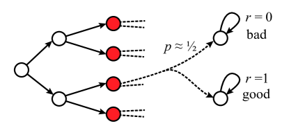
Figure 5: Lower bound construction depicted for $A=2$ actions: This family of MDPs is equivalent to a Bernoulli bandit with $NA$ arms where rewards are scaled by $\bar{H}=\lfloor H-1-\log_{A}N\rfloor$.

For convenience, we restate the theorem statement: See 5

Proof of Theorem 5.

We first specify a family of MDPs that are hard to learn with feedback graphs, then show that learning in hard instances of MABs with $\alpha$ arms can be reduced to learning in this family of MDPs and finally use this reduction to lower bound the regret of any agent.

Family of hard MDPs $\mathcal{M}$:

Without loss of generality, we assume that $N=A^{k}$ for some $k\in\mathbb{N}$.We consider a family $\mathcal{M}$ of $\alpha$ MDPs which are illustrated in Figure 5. Each MDP in $\mathcal{M}$ has $N$ red states (and $N+1$ white states) that form the leaves of a deterministic tree with fan-out $A$. This means that each red state is deterministically reachable by a sequence of actions of length $\lceil\log_{A}N\rceil$. From each red state, the agent transitions to a good absorbing state with certain probability and with remaining probability to a bad absorbing state. All rewards are $0$ except in the good absorbing state where the agent accumulates reward of $1$ until the end of the episode (for a total of $\bar{H}:=H-1-\lceil\log_{A}N\rceil$ time steps).

Let now $G_{1}$ and $G_{2}$ be the feedback graphs for the red and white state-actions respectively. Further let $\mathcal{N}$ be an independent set of $G_{1}$. Each MDP $M_{i}\in\mathcal{M}$ is indexed by an optimal pair $i=(s^{\star},a^{\star})\in\mathcal{N}$ of a red state-action pair. When the agent takes $a^{\star}$ in $s^{\star}$ it transitions to the good state with probability $\delta+\epsilon$. For all other pairs in $\mathcal{N}$, it transitions to the good state with probability $\delta$. All remaining pairs of red states and actions have probability $0$ of reaching the good state. The values of $\delta,\epsilon>0$ will be specified below.

Reduction of learning in MABs to RL in MDPs $\mathcal{M}$:

We now use a reductive argument similar to Mannor and Shamir [33, Theorem 4] to show learning in MABs with $\alpha$ actions cannot me much harder than learning in $\mathcal{M}$.

Let $\mathcal{B}$ be any MDP algorithm and denote by $R_{\mathcal{B},M_{i}}(T)$ its expected regret after $T$ episodes when applied to problem instance $M_{i}\in\mathcal{M}$. We can use $\mathcal{B}$ to construct a multi-armed bandit algorithm $\mathcal{B}^{\prime}$ for a family of MABs $\mathcal{M}^{\prime}$ indexed by $\mathcal{N}$. Each MAB $M^{\prime}_{i}\in\mathcal{M}^{\prime}$ has $|\mathcal{N}|$ arms, all of which have Bernoulli($\delta$) rewards except $i$ which has Bernoulli($\delta+\epsilon$) rewards. To run $\mathcal{B}^{\prime}$ on $M^{\prime}_{i}\in\mathcal{M}^{\prime}$, we apply $\mathcal{B}$ to $M_{i}\in\mathcal{M}$. Whenever $\mathcal{B}$ chooses to execute an episode that visits a $j\in\mathcal{N}$, $\mathcal{B}^{\prime}$ picks arm $j$ in $M^{\prime}_{i}$ and passes on the observed reward as an indicator of whether the good state was reached. When $\mathcal{B}$ chooses to execute an episode that passes through a vertex $x$ of $G_{1}$ that is not in the independent set $\mathcal{N}$, then $\mathcal{B}^{\prime}$ pulls all children $\{y\in\mathcal{N}\colon x\rightarrow_{G_{1}}y\}$ that are in the independent set in an arbitrary order. The observed rewards are again used to construct the observed feedback for $\mathcal{B}$ by interpreting them as indicators for whether the good state was reached.

Lower bound on regret:

We denote by $T^{\prime}$ the (random) number of pulls $\mathcal{B}^{\prime}$ takes until $\mathcal{B}$ has executed $T$ episodes and by $U$ the expected number of times $\mathcal{B}$ plays episodes that do not visit the independent set. The regret of $\mathcal{B}^{\prime}$ after $T^{\prime}$ pulls can then be written as

$$R_{\mathcal{B}^{\prime},M_{i}^{\prime}}(T^{\prime})\leq\frac{R_{\mathcal{B},M_{i}}(T)}{\bar{H}}+\epsilon\alpha U-\delta U,$$ (197)

where the first term $\frac{R_{\mathcal{B},M_{i}}(T)}{\bar{H}}$ is the regret accumulated from pulls where $\mathcal{B}$ visits the independent set and the second term from the pulls where $\mathcal{B}$ did not visit the independent set. Each such episode incurs $\delta$ regret for $\mathcal{B}$ and up to $\alpha\epsilon$ regret for $\mathcal{B}^{\prime}$. We rearrange this inequality as

$$R_{\mathcal{B},M_{i}}(T)\geq\bar{H}(R_{\mathcal{B}^{\prime},M_{i}^{\prime}}(T^{\prime})-\epsilon\alpha U+\delta U)\overset{\leavevmode\hbox to9.15pt{\vbox to9.15pt{\text{[drawing]}}}}{\geq} \bar{H}(R_{\mathcal{B}^{\prime},M_{i}^{\prime}}(T)-\epsilon\alpha U+\delta U)$$ (198)

$$\overset{\leavevmode\hbox to9.15pt{\vbox to9.15pt{\text{[drawing]}}}}{\geq} \bar{H}R_{\mathcal{B}^{\prime},M_{i}^{\prime}}(T)+\bar{H}T[\delta-\epsilon\alpha]^{-},$$ (199)

where follows from monotonicity of regret and from considering the best case $U\in[0,T]$ for algorithm $\mathcal{B}$. The worst-case regret of $\mathcal{B}^{\prime}$ in the $\mathcal{M}^{\prime}$ has been analyzed by Osband and Van Roy [37]. We build on their result and use their Lemma 3 and Proposition 1 to lower bound the regret for $\mathcal{B}^{\prime}$ as follows

$$\max_{i}R_{\mathcal{B}^{\prime},M_{i}^{\prime}}(T)\geq\epsilon T\left(1-\frac{1}{\alpha}-\epsilon\sqrt{\frac{T}{2\delta\alpha}}\right)= \frac{1}{4}\sqrt{\frac{\alpha}{2T}}T\left(1-\frac{1}{\alpha}-\frac{1}{4}\sqrt{\frac{\alpha}{2T}}\sqrt{\frac{4T}{2\alpha}}\right)$$ (200)

$$= \sqrt{\frac{\alpha T}{32}}\left(\frac{3}{4}-\frac{1}{\alpha}\right),$$ (201)

where we set $\delta=\frac{1}{4}$ and $\epsilon=\frac{1}{4}\sqrt{\frac{\alpha}{2T}}$ (which satisfy $\epsilon\leq 1-2\delta$ required by Proposition 1 for $T\geq\alpha/8$). Plugging this result back into (199) gives a worst-case regret bound for $\mathcal{B}$ of

$$\max_{i}R_{\mathcal{B},M_{i}}(T)\geq\sqrt{\frac{\alpha T}{32}}\left(\frac{3}{4}-\frac{1}{\alpha}\right)+\bar{H}T[\delta-\epsilon\alpha]^{-}\geq\bar{H}\sqrt{\frac{\alpha T}{32}}\left(\frac{3}{4}-\frac{1}{\alpha}\right)\geq\frac{H}{32}\sqrt{\frac{\alpha T}{2}},$$ (202)

where we first dropped the second term because $\delta\geq\epsilon\alpha$ for $T\geq\alpha^{3}/8$ and then used the assumptions $\alpha\geq 2$ and $H\geq 2+2\log_{A}N$. ∎

F.2 Lower Sample Complexity Bound with Domination Number

Proof of Theorem 6.

Let $Z=\frac{S}{8}$ and $\bar{Z}=ZA$ which we assume to be integer without loss of generality. The family of MDPs consists of $\bar{Z}\times\bar{Z}$ MDPs, indexed by $(i,j)\in[\bar{Z}]^{2}$. All MDPs have the same structure:

Family of MDPs:

We order $4Z$ states in a deterministic tree so any of the $2Z$ leaf nodes can be reached by a specific action sequence. See Figure 3 for an example with two actions. We split the state-action pairs at the leafs in two sets $\mathcal{B}_{1}=\{x_{1},\dots x_{\bar{Z}}\}$ and $\mathcal{B}_{2}=\{z_{1},\dots z_{\bar{Z}}\}$, each of size $\bar{Z}$. Playing $x_{i}$ transitions to the good absorbing state with some probability $g$ and otherwise to the bad absorbing state $b$. The reward is $0$ in all states and actions, except in the good state $g$, where agent receives a reward of $1$. The transition probabilities from $x_{i}$ depend on the specific MDP. Consider MDP $(j,k)$, then

$$P(g|x_{1})=\frac{1}{2}+\frac{\epsilon}{2H},\qquad\textrm{and,}\qquad P(g|x_{i})=\frac{1}{2}+\frac{\epsilon}{H}{\bf 1}\{i=k\}.$$ (203)

Hence, the first index of the MDP indicates which $x_{i}$ is optimal. Since the agent will stay in the good state for at least $H/2$ time steps (by the assumption that $H\geq 2\log_{A}(S/4)$ by assumption), the agent needs to identify which $x_{i}$ to play in order to identify an $\frac{\epsilon}{4}$-optimal policy. All pairs $z_{i}$ transition to the bad state deterministically, except for pair $z_{j}$ in MDPs $(i,j)$. This pair transitions with probability $p_{0}$ to another tree of states (of size at most $2Z$) which has $\gamma$ state-action pairs at the leafs, denoted by $\mathcal{D}=\{d_{1},\dots,d_{\gamma}\}$. All pairs in this set transition to the bad state deterministically.

The feedback graph is sparse. There are no edges, except each node $d_{i}$ has exactly $\frac{\bar{Z}}{\gamma}$ edges (which we assume to be integer for simplicity) to pairs in $\mathcal{B}_{1}$. No nodes $d_{i}$ and $d_{j}$ point to the same node. Hence, $\mathcal{D}$ forms a dominating set of the feedback graph.

Sample Complexity:

The construction of $\mathcal{B}_{1}$ is equivalent to the multi-armed bandit instances in Theorem 1 by Mannor and Tsitsiklis [34]. Consider any algorithm and let $o_{i}$ be the number of observations an algorithm has received for $x_{i}$ when it terminates. By applying Theorem 1 by Mannor and Tsitsiklis [34], we know that if the algorithm indeed outputs an $\frac{\epsilon}{4}$-optimal policy with probability at least $1-\delta$ in any instance of the family, it has to collect in instances $(1,j)$ at least the following number of samples in expectation

$$\mathbb{E}_{(1,j)}[o_{i}]\geq\frac{c_{1}H^{2}}{\epsilon^{2}}\ln\frac{c_{2}}{\delta}$$ (204)

for some absolute constants $c_{1}$ and $c_{2}$. Let $v(x)$ be the number of times the algorithm actually visited a state-action pair $x$. Then $o_{i}=v(x_{i})+v(d_{j})$ for $j$ with $d_{j}\rightarrow_{G}x_{i}$ because the algorithm can only observe a sample for $x_{i}$ if it actually visits it or the node in the dominating set. Applying this identity to (204) yields

$$\mathbb{E}_{(1,k)}[v(d_{j})]\geq\frac{c_{1}H^{2}}{\epsilon^{2}}\ln\frac{c_{2}}{\delta}-\mathbb{E}_{(1,k)}[v(x_{i})]$$ (205)

for all $d_{j}$ and $x_{i}$ with $d_{j}\rightarrow x_{i}$. Summing over $i\in\bar{Z}$ and using the fact that each $d_{j}$ is counted $\bar{Z}/\gamma$ times, we get

$$\frac{\bar{Z}}{\gamma}\sum_{j=1}^{\gamma}\mathbb{E}_{(1,k)}[v(d_{j})]\geq\frac{c_{1}\bar{Z}H^{2}}{\epsilon^{2}}\ln\frac{c_{2}}{\delta}-\sum_{i=1}^{\bar{Z}}\mathbb{E}_{(1,k)}[v(x_{i})].$$ (206)

After renormalizing, we get,

$$\sum_{j=1}^{\gamma}\mathbb{E}_{(1,k)}[v(d_{j})]\geq\frac{c_{1}\gamma H^{2}}{\epsilon^{2}}\ln\frac{c_{2}}{\delta}-\frac{\gamma}{\bar{Z}}\sum_{i=1}^{\bar{Z}}\mathbb{E}_{(1,k)}[v(x_{i})].$$ (207)

Next, observe that either the algorithm needs to visit nodes in $\mathcal{B}_{1}$ at least $\frac{c_{1}\bar{Z}H^{2}}{2\epsilon^{2}}\ln\frac{c_{2}}{\delta}$ times in expectation or nodes in the dominating set $\mathcal{D}$ at least $\frac{c_{1}\gamma H^{2}}{2\epsilon^{2}}\ln\frac{c_{2}}{\delta}$ times in expectation. The former case gives an expected number of episodes of $\Omega\left(\frac{SAH^{2}}{\epsilon^{2}}\ln\frac{1}{\delta}\right)$ which is the second term in the lower-bound to show.

It remains the case where $\sum_{j=1}^{\gamma}\mathbb{E}_{(1,k)}[v(d_{j})]\geq\frac{c_{1}\gamma H^{2}}{2\epsilon^{2}}\ln\frac{c_{2}}{\delta}$. The algorithm can only reach the dominating set through $z_{k}$ and it can visit only one node in the dominating set per episode. Further, when the algorithm visits $z_{k}$, it only reaches the dominating set with probability $p_{0}$. Hence,

$$\mathbb{E}_{(1,k)}[v(z_{k})]=p_{0}\sum_{j=1}^{\gamma}\mathbb{E}_{(1,k)}[v(d_{j})]\geq\frac{c_{1}\gamma H^{2}}{2p_{0}\epsilon^{2}}\ln\frac{c_{2}}{\delta},$$ (208)

but the algorithm may also visit other pairs $z_{i}$ for $i\neq k$ as well. To see this, consider the expected number of visits to all $z_{i}$s before the algorithm visits the dominating set for the first time. By Lemma 25, this is at least $\frac{\bar{Z}}{4p_{0}}$ in the worst case over $k$. This shows that

$$\max_{k\in[\bar{Z}]}\sum_{i=1}^{\bar{Z}}\mathbb{E}_{(1,k)}[v(z_{i})]\geq\frac{c_{1}\gamma H^{2}}{2p_{0}\epsilon^{2}}\ln\frac{c_{2}}{\delta}-1+\frac{\bar{Z}}{4p_{0}}=\Omega\left(\frac{\gamma H^{2}}{p_{0}\epsilon^{2}}\ln\frac{c_{2}}{\delta}+\frac{SA}{p_{0}}\right).$$ (209)

∎

Lemma 25.

Consider $k$ biased coins, where all but one coin have probability $0$ of showing heads. Only one coin has probability $p$ of showing head. The identity $i$ of this coin is unknown. The expected number of coin tosses $N$ until the first head is for any strategy

$$\mathbb{E}[N]\geq\frac{k}{4p}$$ (210)

in the worst case over $i$.

Proof.

Let $N$ be the number of coin tosses when the first head occurs and let Alg be a strategy. The quantity of interest is

$$\inf_{\textrm{Alg}}\max_{i\in[k]}\mathbb{E}_{t(i)}[\mathbb{E}_{R(\textrm{Alg})}[N]],$$ (211)

where $R(\textrm{Alg})$ denotes the internal randomness of the strategy and $t(i)$ the random outcomes of coin tosses. We first simplify this expression to

$$\inf_{\textrm{Alg}}\max_{i\in[k]}\mathbb{E}_{t(i)}[\mathbb{E}_{R(\textrm{Alg})}[N]] \geq\inf_{\textrm{Alg}}\frac{1}{k}\sum_{i=1}^{k}\mathbb{E}_{t(i)}[\mathbb{E}_{R(\textrm{Alg})}[N]]=\inf_{\textrm{Alg}}\mathbb{E}_{R(\textrm{Alg})}\left[\frac{1}{k}\sum_{i=1}^{k}\mathbb{E}_{t(i)}[N]\right]$$ (212)

$$=\inf_{\textrm{Alg}}\mathbb{E}_{R(\textrm{Alg})}\left[\frac{1}{k}\sum_{i=1}^{k}\sum_{m=0}^{\infty}\mathbb{P}_{t(i)}[N>m]\right]$$ (213)

$$=\inf_{\textrm{Alg}}\mathbb{E}_{R(\textrm{Alg})}\left[\sum_{m=0}^{\infty}\frac{1}{k}\sum_{i=1}^{k}\mathbb{P}_{t(i)}[N>m]\right],$$ (214)

and derive an explicit expression for $\frac{1}{k}\sum_{i=1}^{k}\mathbb{P}_{t(i)}[N>m]$. Since the strategy and its randomness is fixed, it is reduced to a deterministic sequence of coin choices. That is, for a given number of total tosses $N$, a deterministic strategy is the number of tosses of each coin $n_{1},\dots,n_{k}$ with $\sum_{i=1}^{k}n_{i}=N$. Consider any such strategy and let a $n_{1},\dots,n_{k}$ with $\sum_{i=1}^{k}n_{i}=m$ be the coins selected up to $m$. If $N>m$, then the first $n_{i}$ tosses of coin $i$ must be tail. Hence, using the geometric distribution, we can explicitly write the probability of this event as

$$\frac{1}{k}\sum_{i=1}^{k}\mathbb{P}_{t(i)}[N>m]\geq\frac{1}{k}\sum_{i=1}^{k}(1-p)^{n_{i}}\geq\inf_{n_{1:k}\colon\sum_{i=1}^{k}n_{i}=m}\frac{1}{k}\sum_{i=1}^{k}(1-p)^{n_{i}}.$$ (215)

The second inequality just considers the worst-case. The expression on the RHS is a convex program over the simplex with a symmetric objective. The optimum can therefore only be attained at an arbitrary corner of the simplex or the center. The value at the center is $(1-p)^{m/k}$ and by Young’s inequality, we have

$$(1-p)^{m/k}\leq\frac{((1-p)^{m/k})^{k}}{k}+\frac{1^{k/k-1}}{k/(k-1)}=\frac{(1-p)^{m}}{k}+\frac{k-1}{k},$$ (216)

where the RHS is the value of the program at a corner. Hence $\frac{1}{k}\sum_{i=1}^{k}\mathbb{P}_{t(i)}[N>m]\geq(1-p)^{m/k}$ holds and plugging this back into (214) gives

$$\inf_{\textrm{Alg}}\max_{i\in[k]}\mathbb{E}_{t(i)}[\mathbb{E}_{R(\textrm{Alg})}[N]]\geq\sum_{m=0}^{\infty}(1-p)^{m/k}=\frac{1}{1-(1-p)^{1/k}}\geq\frac{k}{4p},$$ (217)

where the last inequality follows from basic algebra and holds for $p<0.5$. For $p\geq 0.5$, the worst case is $\frac{k}{4p}\leq\frac{k}{2}$ anyway because that is the expected number of trials until one can identify a coin with $p=1$. ∎

References

• Alon etย al. [2013] N.ย Alon, N.ย Cesa-Bianchi, C.ย Gentile, and Y.ย Mansour. From bandits to experts: A tale of domination and independence. In Advances in Neural Information Processing Systems, pages 1610โ€“1618, 2013.
• Arora etย al. [2019] R.ย Arora, T.ย V. Marinov, and M.ย Mohri. Bandits with feedback graphs and switching costs. In Advances in Neural Information Processing Systems 32: Annual Conference on Neural Information Processing Systems 2019, NeurIPS 2019, 8-14 December 2019, Vancouver, BC, Canada, pages 10397โ€“10407, 2019.
• Azar etย al. [2012] M.ย G. Azar, R.ย Munos, and H.ย J. Kappen. On the sample complexity of reinforcement learning with a generative model. In Proceedings of the 29th International Coference on International Conference on Machine Learning, pages 1707โ€“1714. Omnipress, 2012.
• Azar etย al. [2017] M.ย G. Azar, I.ย Osband, and R.ย Munos. Minimax regret bounds for reinforcement learning. In International Conference on Machine Learning, pages 263โ€“272, 2017.
• Boutilier etย al. [1999] C.ย Boutilier, T.ย Dean, and S.ย Hanks. Decision-theoretic planning: Structural assumptions and computational leverage. Journal of Artificial Intelligence Research, 11:1โ€“94, 1999.
• Buccapatnam etย al. [2014] S.ย Buccapatnam, A.ย Eryilmaz, and N.ย B. Shroff. Stochastic bandits with side observations on networks. In The 2014 ACM International Conference on Measurement and Modeling of Computer Systems, SIGMETRICS โ€™14, pages 289โ€“300. ACM, 2014.
• Caron etย al. [2012] S.ย Caron, B.ย Kveton, M.ย Lelarge, and S.ย Bhagat. Leveraging side observations in stochastic bandits. In UAI, 2012.
• Cohen etย al. [2016] A.ย Cohen, T.ย Hazan, and T.ย Koren. Online learning with feedback graphs without the graphs. In International Conference on Machine Learning, pages 811โ€“819, 2016.
• Cortes etย al. [2018] C.ย Cortes, G.ย DeSalvo, C.ย Gentile, M.ย Mohri, and S.ย Yang. Online learning with abstention. In 35th ICML, 2018.
• Cortes etย al. [2019] C.ย Cortes, G.ย DeSalvo, C.ย Gentile, M.ย Mohri, and S.ย Yang. Online learning with sleeping experts and feedback graphs. In Proceedings of ICML, pages 1370โ€“1378, 2019.
• Dann [2019] C.ย Dann. Strategic Exploration in Reinforcement Learning - New Algorithms and Learning Guarantees. PhD thesis, Carnegie Mellon University, 2019.
• Dann and Brunskill [2015] C.ย Dann and E.ย Brunskill. Sample complexity of episodic fixed-horizon reinforcement learning. In Advances in Neural Information Processing Systems, pages 2818โ€“2826, 2015.
• Dann etย al. [2017] C.ย Dann, T.ย Lattimore, and E.ย Brunskill. Unifying PAC and regret: Uniform pac bounds for episodic reinforcement learning. In Advances in Neural Information Processing Systems, pages 5713โ€“5723, 2017.
• Dann etย al. [2018] C.ย Dann, N.ย Jiang, A.ย Krishnamurthy, A.ย Agarwal, J.ย Langford, and R.ย E. Schapire. On oracle-efficient PAC reinforcement learning with rich observations. arXiv preprint arXiv:1803.00606, 2018.
• Dann etย al. [2019] C.ย Dann, L.ย Li, W.ย Wei, and E.ย Brunskill. Policy certificates: Towards accountable reinforcement learning. International Conference on Machine Learning, 2019.
• Dong etย al. [2019] S.ย Dong, B.ย Vanย Roy, and Z.ย Zhou. Provably efficient reinforcement learning with aggregated states. arXiv preprint arXiv:1912.06366, 2019.
• Du etย al. [2019] S.ย Du, A.ย Krishnamurthy, N.ย Jiang, A.ย Agarwal, M.ย Dudik, and J.ย Langford. Provably efficient rl with rich observations via latent state decoding. In International Conference on Machine Learning, pages 1665โ€“1674, 2019.
• Goel etย al. [2017] K.ย Goel, C.ย Dann, and E.ย Brunskill. Sample efficient policy search for optimal stopping domains. In Proceedings of the 26th International Joint Conference on Artificial Intelligence, pages 1711โ€“1717. AAAI Press, 2017.
• Henderson etย al. [2017] P.ย Henderson, R.ย Islam, P.ย Bachman, J.ย Pineau, D.ย Precup, and D.ย Meger. Deep reinforcement learning that matters. arXiv preprint arXiv:1709.06560, 2017.
• Howard etย al. [2018] S.ย R. Howard, A.ย Ramdas, J.ย Mcย Auliffe, and J.ย Sekhon. Uniform, nonparametric, non-asymptotic confidence sequences. arXiv preprint arXiv:1810.08240, 2018.
• Jiang etย al. [2017] N.ย Jiang, A.ย Krishnamurthy, A.ย Agarwal, J.ย Langford, and R.ย E. Schapire. Contextual decision processes with low bellman rank are pac-learnable. In International Conference on Machine Learning, pages 1704โ€“1713, 2017.
• Jin etย al. [2018] C.ย Jin, Z.ย Allen-Zhu, S.ย Bubeck, and M.ย I. Jordan. Is Q-learning provably efficient? arXiv preprint arXiv:1807.03765, 2018.
• Jin etย al. [2019] C.ย Jin, Z.ย Yang, Z.ย Wang, and M.ย I. Jordan. Provably efficient reinforcement learning with linear function approximation. arXiv preprint arXiv:1907.05388, 2019.
• Jin etย al. [2020] C.ย Jin, A.ย Krishnamurthy, M.ย Simchowitz, and T.ย Yu. Reward-free exploration for reinforcement learning. arXiv preprint arXiv:2002.02794, 2020.
• Kocรกk etย al. [2016] T.ย Kocรกk, G.ย Neu, and M.ย Valko. Online learning with noisy side observations. In AISTATS, pages 1186โ€“1194, 2016.
• Kostrikov etย al. [2020] I.ย Kostrikov, D.ย Yarats, and R.ย Fergus. Image augmentation is all you need: Regularizing deep reinforcement learning from pixels. arXiv preprint arXiv:2004.13649, 2020.
• Krizhevsky etย al. [2012] A.ย Krizhevsky, I.ย Sutskever, and G.ย E. Hinton. Imagenet classification with deep convolutional neural networks. In Advances in neural information processing systems, pages 1097โ€“1105, 2012.
• Laskin etย al. [2020] M.ย Laskin, K.ย Lee, A.ย Stooke, L.ย Pinto, P.ย Abbeel, and A.ย Srinivas. Reinforcement learning with augmented data. arXiv preprint arXiv:2004.14990, 2020.
• Lattimore and Czepesvari [2018] T.ย Lattimore and C.ย Czepesvari. Bandit Algorithms. Cambridge University Press, 2018.
• Lattimore and Hutter [2012] T.ย Lattimore and M.ย Hutter. PAC bounds for discounted MDPs. In International Conference on Algorithmic Learning Theory, pages 320โ€“334. Springer, 2012.
• Lin etย al. [2019] Y.ย Lin, J.ย Huang, M.ย Zimmer, J.ย Rojas, and P.ย Weng. Towards more sample efficiency in reinforcement learning with data augmentation. arXiv preprint arXiv:1910.09959, 2019.
• Lykouris etย al. [2019] T.ย Lykouris, E.ย Tardos, and D.ย Wali. Graph regret bounds for Thompson sampling and UCB. arXiv preprint arXiv:1905.09898, 2019.
• Mannor and Shamir [2011] S.ย Mannor and O.ย Shamir. From bandits to experts: On the value of side-observations. In Advances in Neural Information Processing Systems, pages 684โ€“692, 2011.
• Mannor and Tsitsiklis [2004] S.ย Mannor and J.ย N. Tsitsiklis. The sample complexity of exploration in the multi-armed bandit problem. Journal of Machine Learning Research, 5(Jun):623โ€“648, 2004.
• Maurer and Pontil [2009] A.ย Maurer and M.ย Pontil. Empirical Bernstein bounds and sample variance penalization. arXiv preprint arXiv:0907.3740, 2009.
• Mnih etย al. [2015] V.ย Mnih, K.ย Kavukcuoglu, D.ย Silver, A.ย A. Rusu, J.ย Veness, M.ย G. Bellemare, A.ย Graves, M.ย Riedmiller, A.ย K. Fidjeland, G.ย Ostrovski, etย al. Human-level control through deep reinforcement learning. Nature, 518(7540):529, 2015.
• Osband and Vanย Roy [2016] I.ย Osband and B.ย Vanย Roy. On lower bounds for regret in reinforcement learning. arXiv preprint arXiv:1608.02732, 2016.
• Ross etย al. [2011] S.ย Ross, G.ย J. Gordon, and J.ย A. Bagnell. A reduction of imitation learning and structured prediction to no-regret online learning. In International Conference on Artificial Intelligence and Statistics, 2011.
• Silver etย al. [2017] D.ย Silver, J.ย Schrittwieser, K.ย Simonyan, I.ย Antonoglou, A.ย Huang, A.ย Guez, T.ย Hubert, L.ย Baker, M.ย Lai, A.ย Bolton, etย al. Mastering the game of go without human knowledge. Nature, 550(7676):354, 2017.
• Simchowitz and Jamieson [2019] M.ย Simchowitz and K.ย Jamieson. Non-asymptotic gap-dependent regret bounds for tabular MDPs. arXiv preprint arXiv:1905.03814, 2019.
• Zanette and Brunskill [2019] A.ย Zanette and E.ย Brunskill. Tighter problem-dependent regret bounds in reinforcement learning without domain knowledge using value function bounds. https://arxiv.org/abs/1901.00210, 2019.
• Zhang etย al. [2017] H.ย Zhang, M.ย Cisse, Y.ย N. Dauphin, and D.ย Lopez-Paz. mixup: Beyond empirical risk minimization. arXiv preprint arXiv:1710.09412, 2017.