A Gaussian Process Upsampling Model for Improvements in Optical Character Recognition

Abstract

Optical Character Recognition and extraction is a key tool in the automatic evaluation of documents in a financial context. However, the image data provided to automated systems can have unreliable quality, and can be inherently low-resolution or downsampled and compressed by a transmitting program. In this paper, we illustrate the efficacy of a Gaussian Process upsampling model for the purposes of improving OCR and extraction through upsampling low resolution documents.

1 Introduction

An important problem in computer vision is the retrieval of textual information from images of documents. This is especially useful for search engines, accessibility tools for the visually impaired, and for processing of financial documents. For these purposes, optical character recognition (OCR) engines have been constructed. The popular open-source OCR framework Tesseract is used in this study. Optical character recognition frameworks, in general, are only as good as the document image that is supplied to them. In many cases, the resolution of the document image plays a role in how well the characters are extracted. In order to better upsample low resolution document images, a new Gaussian Process Modeling upsampling algorithm is constructed and presented in this paper.

This manuscript is organized in the following way. To begin, OCR is introduced along with the state-of-the-art OCR extraction software Tesseract. Next, the Gaussian Process based upsampling method is discussed, along with a brief study on the choice of covariance kernels and the use of a maximum likelihood estimate for the mean. Finally the algorithm is tested against the baseline bicubic upsampling technique by examining the produced OCR accuracy resulting from these upsampled images.

2 Optical Character Recognition

Optical Character Recognition is the conversion of pixel represented words and characters within images into machine-encoded text. As previously mentioned, the OCR framework Tesseract [9] is used to extract text in the document images used in this manuscript. Tesseract was originally formulated by HP research between 1984 and 1994. Since then it has changed hands and now is an open-source software package managed by Google [5] – under the Apache 2.0 License. We use Tesseract 4.1.1, which generates text based utilizing a Long-Short Term Memory (LSTM) network. Tesseract ingests single-channel images and generates feature-maps based on these images. Then these feature maps are embedded into an input for the LSTM [9, 5].

3 The Gaussian Process Algorithm

This interpolation method has taken inspiration from a new interpolation method for computation fluid dynamics proposed in [8]. The authors used a windowed GP method to upsample simulation data from coarse to fine computational meshes. For our application we define text in single-channel document images by pixels with low intensity values (close to 0 or black), surrounded by pixels of high intensity (closer to 255 or white in an 8 bit context). Specifically, pixel values are low in the interior of a character, and pixel values are comparatively high outside of characters. Because of this specific structure, the type of GP modeling will change. Instead of modeling the raw values, the deviation from a mean intensity will be modeled. This allows the upsampling algorithm to better maintain these intensities in the presence of characters. This structure is discussed in more detail in Subsections 3.2 and 3.3. Mathematically, we define the upsampling operator to be

$$f_{*}=f_{0}+\mathbf{k}_{*}^{T}\mathbf{K}^{-1}\left(\mathbf{f}-\bar{\mathbf{f}}\right)$$ (1)

which follows the formula for the posterior mean [7]. In Equation (1), $\mathbf{k}_{*}$ is a vector of covariances between the sample pixel locations and the location of the pixel we wish to interpolate. Furthermore $\mathbf{K}$ is a matrix of pairwise covariances between sample points. The term $f_{0}$ is the estimate for the prior mean pixel intensity over the sample, and $\bar{\mathbf{f}}=f_{0}\mathbf{1}$, calculation of these terms is found in Subsection 3.2. In Subsection 3.1, we discuss the choice of covariance kernel to generate $\mathbf{k}_{*}$ and $\mathbf{K}$.

3.1 Choice of Covariance Kernel

The commonly used squared exponential kernel [7] is often used when the underlying function is continuous and is the de-facto covariance function when building a Gaussian Process. Image data on the other hand, is inherently discontinuous and is comprised of 8 or 16 bit integers. So instead of the SE kernel, a member of Matérn family of kernels is used. In the Matérn family of covariance functions, there are 3 hyper-parameters that dictate their character – as indicated in Equation (2).

$$K_{mat}(\mathbf{x},\mathbf{y})=\Sigma^{2}\frac{2^{1-\nu}}{\Gamma(\nu)}\left(\sqrt{2\nu}\frac{||\mathbf{x}-\mathbf{y}||}{\ell}\right)^{\nu}K_{\nu}\left(\sqrt{2\nu}\frac{||\mathbf{x}-\mathbf{y}||}{\ell}\right)$$ (2)

For the Matérn kernels, there are three hyper-parameters $\Sigma$, $\ell$, and $\nu$. The hyper-parameter $\Sigma$ related to the output variance function, and is widely used for uncertainty quantification. The term $\ell$ is the inherent length scale of covariance in for the underlying function space. The hyper-parameter $\nu$ on the other hand, relates the level of ”continuousness” of the functions that are sampled. The function $K_{\nu}$ is the modified Bessel function of the second kind of order $\nu$. The Matérn family of covariance functions give continuity properties ranging infinitely differentiable functions, as produced by the SE kernel, and nowhere differentiable – such as those generated by the Ornstein-Uhlenbeck covariance kernel.

Consideration of the input and output datatypes of the Gaussian Process are key when choosing or building a covariance function. The datatype for this application are document images, which contain sharp contrasts that are handled better by a low $\nu$ Matérn kernel. The Matérn kernel with $\nu=3/2$ is used in this algorithm. For this specific value, Equation (2) can be simplified. By setting $\nu=3/2$,

$$K_{3/2}(\mathbf{x},\mathbf{y})=\Sigma^{2}\left(1+\sqrt{3}\frac{||\mathbf{x}-\mathbf{y}||}{\ell}\right)\exp\left(-\sqrt{3}\frac{||\mathbf{x}-\mathbf{y}||}{\ell}\right).$$ (3)

We choose $\Sigma=1$ as the uncertainty portion of GP modeling will not be used for this application.

In order to discuss the practical difference between the Matèrn 3/2 kernel and the Squared Exponential, Figures 1(a) and 1(b) are generated utilizing functions from the Scikit Learn framework [6]. These figures contain prior and posterior mean functions of the Gaussian Processes generated using the aforementioned covariance kernels. The prior mean functions sampled from the Gaussian Processes offer illustrations of typical functions that ”live” in the function spaces that the covariance kernels expect. The sampled response variable follows the formula $Y=\sin\left((X-2.5)^{2}\right)$, with 10 independent variable samples that follow $X\sim\mathcal{U}(0,5)$. Figure 1(a) contains the prior and posterior mean functions generated from Gaussian Process with the SE Kernel using these response and independent variables.

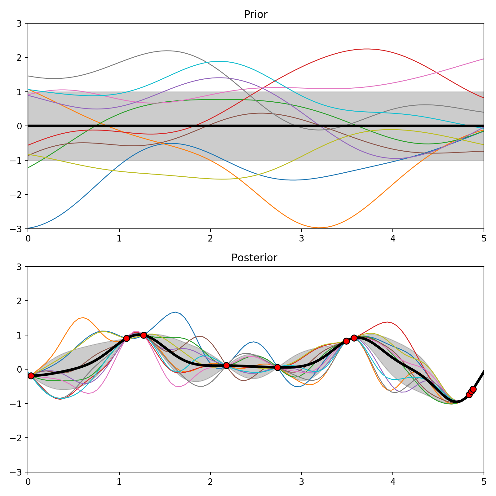
(a) Top: Prior Mean functions. Bottom: Posterior mean functions.

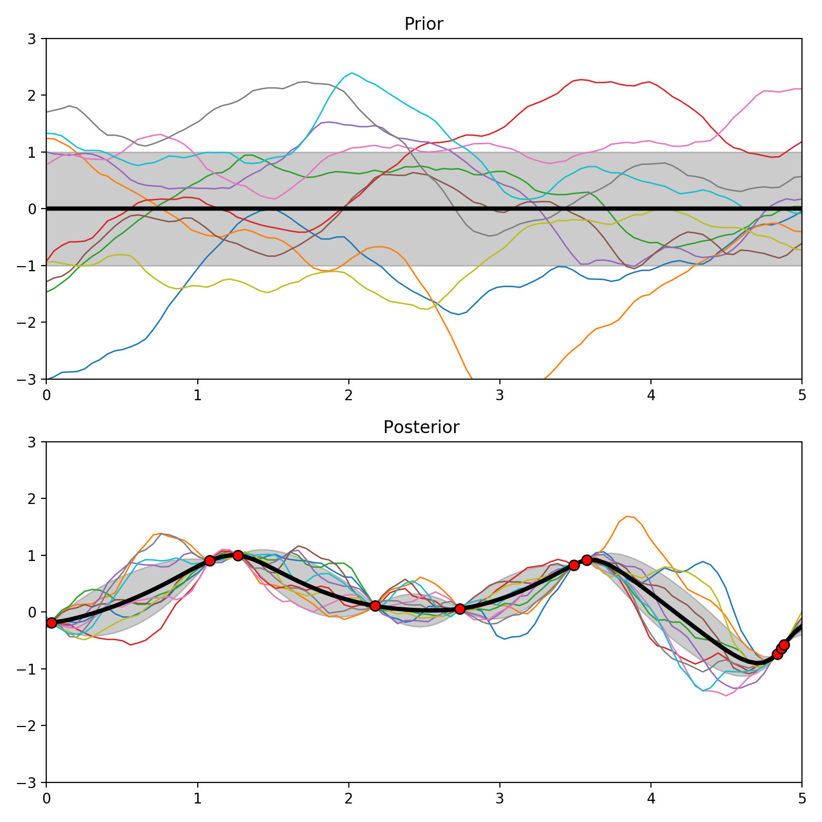
(b) Top: Prior Mean functions. Bottom: Posterior mean functions.

Figure 1: Two Gaussian Processes fitted to 10 samples. Left: GP model with Squared Exponential Kernel, Right: GP model with Matèrn.

The gray space represents the uncertainty of the Gaussian Process models. For Figure 1(b) the above process is repeated utilizing the Matèrn 3/2 kernel instead of SE. Note that in Figure 1(a), the prior and posterior mean functions are much smoother than the functions sampled from and produced by the GP with the Matérn kernel, as represented in Figure 1(b).

3.2 Maximum Likelihood Estimate for the Prior Mean

The prior mean function that will be used is the maximum likelihood estimate for the prior mean, calculated over the $5\times 5$ square patch of pixels. This is done to change the character of the upsampling model so the model predicts the variation about the mean intensity in each sample. Typically, non-zero mean functions are used when there is an observed or assumed trend in the data. In the case of document images, pixel data is expected to retain certain intensities when inside a character or in the white space of a document. Because of these characteristics, a constant non-zero mean is chosen. Note that the derived prior mean functions is only constant over a single window, the prior mean will be constructed over each sample varies over the image.

To calculate the maximum likelihood estimate (MLE) for a constant prior mean, $\bar{\mathbf{f}}=f_{0}\mathbf{1}$, the Gaussian log-likelihood function is optimized with respect to $f_{0}$. The log-likelihood is

$$\ln\mathcal{L}=-\frac{1}{2}\left(\mathbf{f}-\bar{\mathbf{f}}\right)^{T}\mathbf{K}^{T}\left(\mathbf{f}-\bar{\mathbf{f}}\right)-\frac{1}{2}\ln(\det|\mathbf{K}|)-\frac{N}{2}\ln(2\pi).$$ (4)

The maximum is calculated by setting the derivative of Equation 4 with respect to $f_{0}$ and solving for $f_{0}$. Therefore the maximum likelihood estimate for the prior mean is:

$$f_{0}=\frac{\mathbf{1}^{T}\mathbf{K}^{-1}\mathbf{f}}{\mathbf{1}^{T}\mathbf{K}^{-1}\mathbf{1}}.$$ (5)

Also, this maximum likelihood estimate for the prior mean can be recast as

$$f_{0}=\frac{\left(\sum_{i}\mathbf{K}^{-1}_{[i]}\right)\cdot\mathbf{f}}{\sum_{i,j}\mathbf{K}^{-1}_{[i,j]}}.$$

This interpretation is simply a weighted average with respect to the GP model.

3.3 Algorithm

In this upsampling algorithm, single channel grayscale document images are used. The Gaussian Process upsampling algorithm begins with the construction of the model weights with a length scale parameter derived from the original resolution of the image - $\ell=20\min(1/h,1/w)$. The upsampling ratio dictates the number of weight vectors needed, for example, when upsampling $4\times$, 16 new pixels are generated and therefore 16 weight vectors are needed. These vectors are generated by utilizing the Cholesky factorization of $\mathbf{K}$ and then applying back substitution to calculate each $\mathbf{k}_{*}^{T}\mathbf{K}^{-1}$. The key factor is that the covariance kernel utilized in this methodology is isotropic– it only depends on the distance between samples. Since a sliding window is used, the upsampling weights only need to be calculated once and can be used throughout the image. This is because the distance between sample pixels are related to their pixel index $(i,j)$ and the distance between each of the upsampled pixels and the rest of the window is identical for every window.

When performing upsampling over the document image, a sliding $5\times 5$ pixel window is used as the sample for the GP model. Figure 2 helps illustrate the sliding window GP method. The figure contains 3 grids of pixels. The first grid represents the constant maximum likelihood estimate for the prior mean over this pixel grid. The second grid represents the deviation of the sampled pixel values from the MLE. Together, these grids combine to interpolate 16 new pixels, replacing the pixel in the $(i,j)$ location.

In the implementation of this algorithm, the maximum likelihood estimate for the prior mean is generated when the $5\times 5$ sample is loaded. Then each GP weight vector $\mathbf{k}_{*}^{T}\mathbf{K}^{-1}$ is applied to the residual between the MLE and pixels in the sampled window to model the deviation. The deviation and the MLE are combined to generate each new pixel $f_{*}$.

Figure 2: Schematic for the 5$\times$5 GP model for 4$\times$ upsampling. The completely gray grid illustrates the computation of $f_{0}$ over the sample, while the GP model combination on the second grid. The last grid illustrates the 16 new $f_{*}$ generated by combining the two, effectively replacing the pixel $(i,j)$

As an example, Figure 3 is used to illustrate the upsampling results utilizing this Gaussian Processes algorithm. The top image in the figure is the low resolution image (resized by copying the nearest pixels to be the same size as the GP image), and bottom text is from the GP upsampled image. When Tesseract is used on these images, it yields the following texts. The low resolution image Tesseract output is:

”desigm £rédacimice en fiflanEm, Et le chiet”,

which is not an accurate representation of the ground truth. However, for the GP upsampled image, Tesseract generates

”design et regactnce en $<<$ Azzmuts $>>$. est le chef”.

It is clear that the GP upsampled version is much closer to the ground truth text of

”design et rédactrice en $<<$Azimuts $>>$, est le chef”.

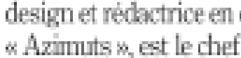
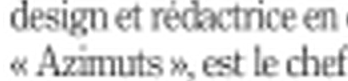
Figure 3: Section of Page 154 of the LRDE dataset. Top: $4\times$ downsampled image crop. Bottom: $4\times$ GP upsampled.

Tesseract works best when used on near-binary images as an input. In this case, near binary means that the majority of the pixels in the image are close to $0$ if they are within a character, or $255$ if not. However, sometimes the single channel images are calculated from RGB images that yield other shades of gray. In this case some images processing techniques can be used to better “binarize” these images. Aside from binarization, images can contain noise or textures within them, which can negatively effect the detection of characters. A common way to handle excess noise and textures is to use a blurring operation to smooth out those regions. However, utilizing these blur convolutions can lead to unwanted removal of edges.

To remove noise and textures without compromising edges the bilateral filtering approach illustrated by Tomasi and Manduchi is used [10]. Bilateral filters reduce noise and textures without compromising edges, that is, without compromising the upsampled edges generated in the GP upsampling.

If the image is not approximately binary, a thresholding technique can be used to force the text to be truly black. An adaptive Gaussian threshold process is used to generate binary images. Thresholding utilizes a set intensity value and replaces all pixels below that value to black and all pixels above the threshold to white. If there are shadows in the image, global thresholding can lead to large portions of the image to be blacked out. This could result in the majority of words in a document image to become inaccessible. An adaptive-thresholding technique utilizes a neighborhood of pixels and calculates the threshold value locally to perform binarization. With Adaptive Gaussian thresholding, the threshold value is the weighted sum of neighborhood pixels in a Gaussian window [2, 1].

Figure 4 contains the results of the pipeline for processing low resolution images and is a visual explanation why filtering is necessary, especially when performing binarization. The top image is a GP upsampled version of a noisy low resolution image. The middle image is a thresholded version of the noisy image without using the bilateral image filter. Binarization, in this case, enhances the inherent noise, resulting in Tesseract to detect no characters. The bottom image is the noisy input image with bilateral filtering applied, and then thresholded. With the last image the Tesseract engine can detect every character.

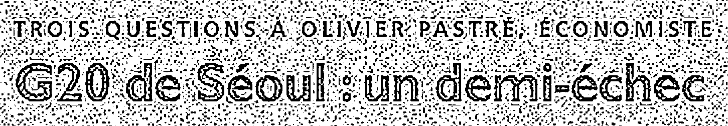
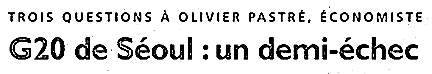
Figure 4: Top: Noisy grayscale GP upsampled text block. Middle: Adaptive thresholding with no filter. Bottom: GP upsampled image with bilateral filter and adaptive thresholding.

The OCR pipeline used is as follows. First, a low resolution image is upsampled using the GP model presented earlier. Then, noise and unwanted textures from the high resolution image are removed while preserving edges by utilizing bilateral filtering. After the GP upsampled image is filtered, if the image is not approximately binary, an adaptive thresholding technique is used to convert the filtered high resolution image into a binary image to be ingested by the Tesseract OCR engine. For clarity, Figure 5 contains an algorithmic diagram with each process.

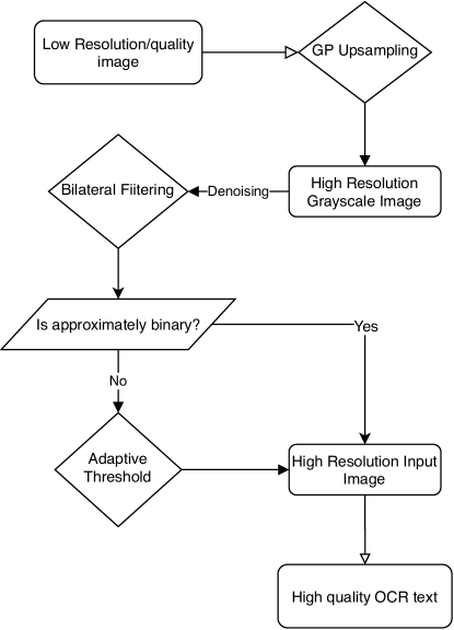
Figure 5: The image processing pipeline used for higher quality OCR.

4 Testing

In order to test the methodology, the EPITA Research and Development Laboratory (LRDE) dataset from [4] is used. This dataset is publicly available but is copyrighted, ©2012 EPITA Research and Development Laboratory (LRDE) with permission from Le Nouvel Observateur. This dataset is based on the French magazine Le Nouvel Observateur, issue 2402, November 18th-2th, 2010. The original images come from this magazine, and LRDE has generated the ground truth OCR from these images. This dataset is free for research, evaluation, and illustration and can be downloaded from LRDE’s website.

To test the proposed GP upsampling algorithm, the original images’ resolution is downsampled $4\times$ in width and height. Then these low resolution representations are combined with Gaussian noise. Next, the noisy low resolution images are upsampled using the GP method illustrated in this manuscript. Finally, the upsampled images are then passed through the image processing pipeline illustrated in Figure 5, to extract detected characters.

For this purpose, accuracy is calculated by comparing the number of words detected in the upsampled document to those that are present in the ground truth text. This is a fairly conservative measure, as increased accuracy in upsampling can lead to increased similarity in generated words with the true words. However, in this case, number of true words matched is a more direct measurement of accuracy that will effect applications that utilize image extracted text.

First, the accuracy of the GP method is compared to the OCR extracted utilizing the low resolution images. Figure 6 contains a graph comparing the accuracy of OCR obtained from the GP upsampled images against OCR from the low resolution images, for each image in the dataset. In the figure, the blue line represents the OCR accuracy for each GP upsampled image, whereas the red line is the OCR accuracy of the low resolution images. Flat dashed lines are included to illustrate the mean accuracy of each set. There are several dips in the graph where both the upsampled accuracy and the low resolution accuracy are very low, these pages of the magazine are comprised of mostly images where text is not the dominant feature. The extraneous information limits the capabilities of the Tesseract OCR engine.

Figure 6: GP upsampled OCR accuracy vs the Low Resolution accuracy with dashed lines denoting average accuracies.

Most applications that require OCR will upsample sufficiently low resolution images. So, naturally, the GP algorithm is compared against the bicubic interpolation method, a common baseline in upsampling algorithms. For this implementation the bicubic method used is contained in the Python Image Library [3]. In this test, the text generated by the GP based pipeline is compared against an analogous bicubic interpolation based pipeline. Figure 7 contains a plot of the relative gain in accuracy when utilizing GP over bicubic interpolation over the LRDE dataset. In the figure, the relative gain is depicted by the blue dots for each image in the dataset. Additionally, a line denoting equal performance is plotted as an orange line for reference. For the majority of images, the proposed algorithm’s extracted text better matches the ground truth text over the baseline interpolation.

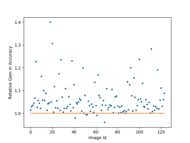
Figure 7: The relative gain utilizing GP upsampling vs bicubic over the noisy low resolution test set. The blue dots are the individual accuracy gains, and a reference line corresponding to equal accuracy is plotted in orange.

Some summary statistics are included in Table 1. The GP algorithm performs the best over the base low resoution images, and the bicubic interpolation based pipeline. The GP algorithm had the highest average accuracy, lowest variance and the highest minimum and maximum accuracy out of the three tests. The last column in the table is the relative gain in OCR accuracy by using the GP algorithm instead of Bicubic or just using the low resolution image. There is a $6.26\%$ increase in character recognition against the bicubic upsampling.

Table 1: Summary statistics of the OCR accuracy over the LRDE subsampled dataset.

	Average	Variance	Max	Min	GP Relative Increase
GP	0.735020	0.012018	0.844515	0.214765	N/A
Bicubic	0.695874	0.013746	0.835996	0.175597	6.26%
Low Resolution	0.345170	0.014018	0.725663	0.003584	195%

5 Conclusion

In this paper, a new Gaussian Process based interpolation model was produced for the explicit purpose of upsampling single-channel document images. Testing over a real-word data set revealed an increase in OCR accuracy over the baseline upsampling method, bicubic interpolation, when used in conjunction with the Tesseract OCR engine.

One could build a Gaussian Process model over the entire low resolution image and generate new pixels with inputs in a non-local sense. This provides issues in multiple areas. The kernel utilized in this context decay rapidly as distance is increased, so the new information gained will become less of a contribution than a hinderance when it comes to computation. Even though the weights are calculated using the Cholesky Factorization of the covariance matrix $\mathbf{K}$, the computational complexity of factorization is still $n^{3}/3$ where $n$ is the size of row and column size of $\mathbf{K}$ [11]. So even on a relatively small resolution image, say $500\times 500$, $\mathbf{K}$ will have size 250000, which will require $5.208\times 10^{15}$ operations. This is realistically infeasible, which leads well into the approach described in this paper. The windowed GP model can be reinterpreted as a Sparse Gaussian Processes that only utilizes information that is local to the interpolation pixels, which will have the most relevant information in both models.

Some minor improvements could be gained by optimizing the length scale parameter, which could be found by maximizing the log-likelihood with respect to $\ell$. However, each window may have a different optimal length scale, which again, leads to an unwanted increase in computational complexity. Additionally, one can tune $\ell$ for the dataset, but the value in this paper appears to be general, as it depends on the size of the low resolution image.

Utilizing the proposed GP algorithm as an upsampling method for Optical Character Recognition yields on average a positive gain in accuracy versus a more traditional bicubic method when used to upsample the images for inputs to the Tesseract OCR engine. The GP algorithm uses a sliding window of $5\times 5$ pixel sampled across the image. The yield in accuracy against bicubic can help text based Natural Language Processing (NLP) models become perform better when placed in an end-to-end environment, like in financial applications, or for accessibility of documents and scanned images for people who are visually impaired.

References

- [1] G. Bradski, The OpenCV Library, Dr. Dobb’s Journal of Software Tools, (2000).
- [2] J. S. III, Spectral audio signal processing, 2011.
- [3] R. Keys, Cubic convolution interpolation for digital image processing, IEEE Transactions on Acoustics, Speech, and Signal Processing, 29 (1981).
- [4] G. Lazzara, R. Levillain, T. Géraud, Y. Jacquelet, J. Marquegnies, and A. Crepin-Leblond, The scribo module of the olena platform: A free software framework for document image analysis, 2011 International Conference on Document Analysis and Recognition, (2011), pp. 252–258.
- [5] C. I. Patel, A. Patel, and D. T. Patel, Optical character recognition by open source ocr tool tesseract: A case study, 2012.
- [6] F. Pedregosa, G. Varoquaux, A. Gramfort, V. Michel, B. Thirion, O. Grisel, M. Blondel, P. Prettenhofer, R. Weiss, V. Dubourg, J. Vanderplas, A. Passos, D. Cournapeau, M. Brucher, M. Perrot, and E. Duchesnay, Scikit-learn: Machine learning in Python, Journal of Machine Learning Research, 12 (2011), pp. 2825–2830.
- [7] C. Rasmussen and C. Williams, Gaussian Processes for Machine Learning, Adaptive Computation And Machine Learning, MIT Press, 2005.
- [8] S. I. Reeves, D. Lee, A. Reyes, C. Graziani, and P. Tzeferacors, An application of gaussian process modeling for adaptive mesh refinement, CAMCOS, (2020).
- [9] R. Smith, An overview of the tesseract ocr engine, in Proc. Ninth Int. Conference on Document Analysis and Recognition (ICDAR), 2007, pp. 629–633.
- [10] C. Tomasi and R. Manduchi, Bilateral filtering for gray and color images, 1998, pp. 839–846.
- [11] L. Trefethen and D. Bau, Numerical linear Algrebra., Society for Industrial and Applied Mathematics, 1997.