On Inexact Accelerated Proximal Gradient Methods with Relative Error Rules

Abstract

One of the most popular and important first-order iterations that provides optimal complexity of the classical proximal gradient method (PGM) is the ‘‘Fast Iterative Shrinkage/Thresholding Algorithm’’ (FISTA). In this paper, two inexact versions of FISTA for minimizing the sum of two convex functions are studied. The proposed schemes inexactly solve their subproblems by using relative error criteria instead of exogenous and diminishing error rules. When the evaluation of the proximal operator is difficult, inexact versions of FISTA are necessary and the relative error rules proposed here may have certain advantages over previous error rules. The same optimal convergence rate of FISTA is recovered for both proposed schemes. Some numerical experiments are reported to illustrate the numerical behavior of the new approaches.

47H05, 47J22, 49M27, 90C25, 90C30, 90C60, 65K10.

1 Introduction

Throughout this paper, we write $p\coloneqq q$ to indicate that $p$ is defined to be equal to $q$. The nonnegative (positive) numbers will be denoted by $\mathbb{R}_{+}$ ($\mathbb{R}_{++}$). Moreover, $\mathbb{E}$ denotes a finite-dimensional real vector space, which is equipped with the inner product $\left\langle{\,\cdot\,},{\cdot\,}\right\rangle$ and its induced norm $\|\cdot\|$.

Consider the following problem

(1) $$\min_{x\in\mathbb{E}}F(x)\coloneqq f(x)+g(x),$$

where $f\colon\mathbb{E}\to\mathbb{R}$ is a differentiable convex function whose gradient is $L$-Lipschitz continuous and $g\colon\mathbb{E}\to\overline{\mathbb{R}}\coloneqq\mathbb{R}\cup\{+\infty\}$ is a lower semicontinuous (lsc) convex function that is not necessarily differentiable. We denote the optimal value of Eq. 1 by $F^{*}$, the set of optimal solutions of Eq. 1 by $S_{*}$, and we assume that $F^{*}\in\mathbb{R}$ and that $S_{*}$ is nonempty; thus we have $F(x_{*})=F^{*}$, for all $x_{*}\in S_{*}$. It is well-known that Eq. 1 contains a wide class of problems arising in applications from science and engineering, including machine learning, compressed sensing, and image processing. There are important examples of this problem such as using $\ell_{1}$--regularization to obtain sparse solutions with applications in signal recovery and signal processing problems [9, 18, 33], the nearest correlation matrix problem [14, 19, 29], and regularized inverse problems with atomic norms [34].

A plethora of methods has been proposed for solving the aforementioned optimization problem. One of the most studied approaches is the proximal gradient method (PGM) which is a first-order splitting iteration that has been intensively investigated in the literature; see, for instance, [8, 11, 12]. PGM iterates by performing a gradient step based on $f$ followed by the evaluation of the proximal (or $\operatorname{Prox}$) operator of $g$, which is defined as $\operatorname{Prox}_{g}\coloneqq(\operatorname{Id}+\partial g)^{-1}$ where

$$\partial g(x)\coloneqq\bigl{\{}u\in\mathbb{E}\bigm{|}g(y)\geq g(x)+\langle u,y-x\rangle,\forall y\in\mathbb{E}\bigr{\}}$$

is the subdifferential of $g$ at $x\in\mathbb{E}$ and $\operatorname{Id}$ is the identity operator. It is well-known that the sequence $(x_{k})_{k\in\mathbb{N}}$ generated by PGM has a complexity rate of $\mathcal{O}(\rho^{-1})$ to obtain a $\rho$--approximate solution of Eq. 1 (that is, a solution $x_{k}$ satisfying $F(x_{k})-F^{*}\leq\rho$), or equivalently we can say that $F(x_{k})-F^{*}=\mathcal{O}(k^{-1})$; see, for instance, [8, 11, 12]. In addition, it is possible to accelerate the proximal gradient method in order to achieve the optimal $\mathcal{O}(k^{-2})$ convergence rate by adding an extrapolation step. This scheme, which improved the complexity of the gradient method for minimizing smooth convex functions, was first introduced by Nesterov in 1983 [25] and further extended to constrained problems in 1988 [26, 27]. In the spirit of the work of [25], Nesterov [28] (appeared online in 2007 but published in 2013) and Beck--Teboulle [8] extended Nesterov’s classical iteration to minimizing composite nonsmooth functions.

In this paper, we propose a modification of the ‘‘Fast Iterative Shrinkage/Thresholding Algorithm’’ (FISTA) of [8]. FISTA is described as follows.

Algorithm 1 (FISTA).

Let $x_{0}\in\mathbb{E}$, and $L>0$ be the Lipschitz constant of $\nabla f$. Set $y_{1}\coloneqq x_{0}$, $t_{1}\coloneqq 1$, and iterate (2) $\displaystyle x_{k}$ $\displaystyle\coloneqq\operatorname{Prox}_{\frac{1}{L}g}\left(y_{k}-\frac{1}{L}\nabla f(y_{k})\right),$ (3) $\displaystyle t_{k+1}$ $\displaystyle\coloneqq\frac{1+\sqrt{1+4t_{k}^{2}}}{2},$ (4) $\displaystyle y_{k+1}$ $\displaystyle\displaystyle\coloneqq x_{k}+\frac{t_{k}-1}{t_{k+1}}(x_{k}-x_{k-1}).$

Note that if the update Eq. 3 is ignored and $t_{k}=1$ for all $k\in\mathbb{N}$, FISTA becomes the (unaccelerated) PGM mentioned before. There are two very popular choices for the sequence $(t_{k})_{k\in\mathbb{N}}$ [8, 28] but several different updates are possible for $t_{k}$ that also achieve the optimal acceleration; see, for instance, [4, 5, 15, 32]. Convergence and complexity results of the sequence generated by FISTA under a suitable tuning of $(t_{k})_{k\in\mathbb{N}}$ related to the update Eq. 3 can be found in [2, 5, 12, 15]. Many accelerated versions have been proposed in the literature for accelerating the PGM for solving Eq. 1. The relaxed case was considered in [6] and error-tolerant versions were studied in [3, 4]. In addition, for results concerning the rate of convergence of function values of Eq. 1 with or without minimizers, see [7, 32].

FISTA (and in particular PGM) is an effective and simple choice for solving large scale problems when the $\operatorname{Prox}$ operator has a closed-form or there exists an efficient way to evaluate it. Frequently, it could be computationally expensive to evaluate the $\operatorname{Prox}$ operator at any point with high accuracy [10]. The theory of convergence for the (accelerated) PGM assumes that the $\operatorname{Prox}$ operator can be evaluated at any point; that is, the regularized minimization problem

$$\min_{x\in\mathbb{E}}\left\{g(x)+\frac{1}{2\gamma}\|x-z\|^{2}\right\},\quad\gamma>0,$$

can be solved for any $z\in\mathbb{E}$. The unique solution of the above problem is actually the $\operatorname{Prox}$ operator of $\gamma g$ at $z$, which is the function $\operatorname{Prox}_{\gamma g}\colon\mathbb{E}\to\operatorname{dom}g$ defined by

$$\operatorname{Prox}_{\gamma g}(z)\coloneqq\operatorname*{argmin}_{x\in\mathbb{E}}\left\{g(x)+\frac{1}{2\gamma}\|x-z\|^{2}\right\}.$$

This function satisfies the following necessary and sufficient optimality condition:

$$\frac{1}{\gamma}\left(z-\operatorname{Prox}_{\gamma g}(z)\right)\in\partial g(\operatorname{Prox}_{\gamma g}(z)).$$

Therefore, to run FISTA we must compute $x_{k}$ by solving the subproblem

(5) $$\min_{x\in\mathbb{E}}\left\{g(x)+\frac{L}{2}\left\|x-\left(y_{k}-\frac{1}{L}\nabla f(y_{k})\right)\right\|^{2}\right\}.$$

That is, we must find the point $x_{k}$ that satisfies

$$0\in\partial g(x_{k})+L(x_{k}-y_{k})+\nabla f(y_{k}).$$

A natural question is: What happens if the solution of Eq. 5 can not be easily computed? Often in practice in this case the evaluation of the proximal operator is done approximately. However, to guarantee an optimal complexity rate, it is required that the nonnegative sequence of error tolerances be summable. As was shown in [19, 34], with a summable sequence of error tolerances for these approximate solutions, the optimal complexity rate $\mathcal{O}(k^{-2})$ of FISTA is recovered.

The two works [19, 34] appeared simultaneously around 2013 and proposed inexact variations of FISTA with summable error tolerances for computing the $\varepsilon$--approximate solutions of subproblem Eq. 5. In [34], given a nonnegative sequence $(\varepsilon_{k})_{k\in\mathbb{N}}$, iterates $\tilde{x}_{k}$ are generated such that

(6) $$0\in\partial_{\varepsilon_{k}}g(\tilde{x}_{k})+L(\tilde{x}_{k}-y_{k})+\nabla f(y_{k}),$$

where

$$\partial_{\varepsilon}g(x)\coloneqq\bigl{\{}u\in\mathbb{E}\bigm{|}g(y)\geq g(x)+\langle{u},{y-x}\rangle-\varepsilon,\forall y\in\mathbb{E}\bigr{\}}$$

is an enlargement of $\partial g$. On the other hand, the version in [19] allows the approximate solution $\tilde{x}_{k}$ of subproblem Eq. 5 such that

(7) $$F(\tilde{x}_{k})\leq g(\tilde{x}_{k})+f(y_{k})+\langle{\nabla f(y_{k})},{\tilde{x}_{k}-y_{k}}\rangle+\langle{\tilde{x}_{k}-y_{k}},{H_{k}(\tilde{x}_{k}-y_{k})}\rangle+\frac{\xi_{k}}{2t_{k}^{2}},$$

$$v_{k}\in\partial_{\frac{\xi_{k}}{2t_{k}^{2}}}g(\tilde{x}_{k})+H_{k}(\tilde{x}_{k}-y_{k})+\nabla f(y_{k}),\quad\|H_{k}^{-1/2}v_{k}\|\leq\frac{\delta_{k}}{\sqrt{2}t_{k}},$$

where $(\delta_{k})_{k\in\mathbb{N}}$ and $(\xi_{k})_{k\in\mathbb{N}}$ are summable sequences of nonnegative numbers, and $H_{k}$ is a self-adjoint positive definite operator. If $H_{k}=L\operatorname{Id}$, then inequality (7) is trivially satisfied. In both of these approaches, the summability assumption may require us to find $\tilde{x}_{k}$ to a level of accuracy that is higher than necessary.

In the spirit of [21, 31], we propose two inexact versions with relative error rules for solving the main subproblem of FISTA. The advantages over the inexact methods given in [19, 34] are the following:

• The proposed relative error rules have no summability assumption and the error tolerances naturally depend on the generated iterates. Our first proposed method is a generalization of FISTA and our second proposed method is related to the extra-step acceleration method proposed in [22].

• We recover the optimal iteration convergence rate in terms of the objective function value for both proposed inexact methods. Moreover, for a given tolerance $\rho>0$, we also study iteration-complexity bounds for the proposed algorithms in order to obtain a $\rho$--approximate solution $x$ of the inclusion $0\in\partial F(x)$ with residual $(r,\varepsilon)$, i.e.,

  $$r\in\partial_{\varepsilon}F(x),\quad\max\{\|r\|,\varepsilon\}\leq\rho.$$

  Since $0\in\partial F(x_{*})$, for all $x_{*}\in S_{*}$, the latter condition can be interpreted as an optimality measure for $x$.

The presentation of this paper is as follows. Definitions, basic facts and auxiliary results are presented in Section 2. Our inexact criteria with relative error rules are presented in Section 3. In Sections 4 and 5 we present the inexact algorithms and their convergence rates. Some numerical experiments for the proposed schemes are reported in Section 6. Finally, some concluding remarks are given in Section 7.

2 Definitions and auxiliary results

Let $h\colon\mathbb{E}\to\overline{\mathbb{R}}$ be a proper, convex, and lower semicontinuous (l.s.c.) function. We denote the domain of $h$ by $\operatorname{dom}h\coloneqq\{x\in\mathbb{E}\mid h(x)<+\infty\}$. Recall that the proximal operator $\operatorname{Prox}_{h}\colon\mathbb{E}\to\operatorname{dom}g$ is defined by $\operatorname{Prox}_{h}(x):=(\operatorname{Id}+\partial h)^{-1}(x)$. It is well-known that the proximal operator is single-valued with full domain, is continuous, and has many other attractive properties. In particular, the proximal operator is firmly nonexpansive:

$$\left\|\operatorname{Prox}_{h}(x)-\operatorname{Prox}_{h}(y)\right\|^{2}\leq\|x-y\|^{2}-\left\|(x-\operatorname{Prox}_{h}(x))-(y-\operatorname{Prox}_{h}(y))\right\|^{2},$$

for all $x,y\in\mathbb{E}$. Moreover,

$$0\in\partial g(\operatorname{Prox}_{\gamma h}(x))+\frac{1}{\gamma}\left(\operatorname{Prox}_{\gamma h}(x)-x\right),\quad x\in\mathbb{E},\,\gamma>0.$$

We let $J\colon{\mathbb{E}}\times\mathbb{R}_{++}\to\operatorname{dom}g$ be the forward-backward operator for problem Eq. 1, which is given by

(8) $$J(x,\gamma):=\operatorname{Prox}_{\gamma g}(x-\gamma\nabla f(x)),\quad x\in\mathbb{E},\,\gamma>0.$$

It is well known that if $h$ is differentiable and $\nabla h$ is $L$-Lipschitz continuous on $\mathbb{E}$, i.e.,

$$\|\nabla h(x)-\nabla h(y)\|\leq L\|x-y\|,\quad x,y\in\mathbb{E},$$

then, for all $x,y\in\mathbb{E}$, we have

(9) $$h(y)+\langle\nabla h(y),x-y\rangle\leq h(x)\leq h(y)+\langle\nabla h(y),x-y\rangle+\frac{L}{2}\|x-y\|^{2}.$$

The next lemma provides some basic properties of the subdifferential operator.

Lemma 2.1.

Let $h,f\colon\mathbb{E}\to\overline{\mathbb{R}}$ be proper, closed, and convex functions. Then:

$\partial_{\varepsilon}h(x)+\partial_{\mu}f(x)\subset\partial_{\varepsilon+\mu}(h+f)(x)$, for all $x\in\mathbb{E}$ and $\varepsilon,\mu\geq 0$.

$w\in\partial h(y)$ implies $w\in\partial_{\varepsilon}h(x)$, where $\varepsilon=h(x)-[h(y)+\langle{w},{x-y}\rangle]\geq 0$.

The following notion of an approximate solution of problem Eq. 1 is used in the complexity analysis of our methods.

Definition 2.2.

Given a tolerance $\rho>0$, a point $x\in\mathbb{R}^{n}$ is said to be a $\rho$-approximate solution of problem Eq. 1 with residues $(v,\varepsilon)\in\mathbb{R}^{n}\times\mathbb{R}_{+}$ if and only if

$$v\in\partial_{\varepsilon}F(x),\quad\max\{\|v\|,\varepsilon\}\leq\rho.$$

We end this section by presenting some elementary properties on the extrapolate sequences used by the proposed methods.

Lemma 2.3.

The positive sequence $(t_{k})_{k\in{\mathbb{N}}}$ generated by Eq. 3 satisfies, for all $k\in\mathbb{N}$,

$\displaystyle\frac{1}{t_{k}}\leq\frac{2}{k+1}$,

$\displaystyle t^{2}_{k+1}-t_{k+1}=t^{2}_{k}$,

$\displaystyle 0\leq\frac{t_{k}-1}{t_{k+1}}\leq 1$.

Lemma 2.4.

Let $\lambda\geq 1$ be given. The sequence $(\tau_{k})_{k\in{\mathbb{N}}}$ recursively defined by

(10) $$\tau_{0}\coloneqq 0,\quad\mbox{and}\quad\tau_{k+1}\coloneqq\tau_{k}+\frac{\lambda+\sqrt{\lambda^{2}+4\lambda\tau_{k}}}{2},$$

satisfies, for all $k\in\mathbb{N}$,

$\tau_{k+1}>\tau_{k}$ and $\displaystyle\frac{\tau_{k+1}}{{(\tau_{k+1}-\tau_{k}})^{2}}=\frac{1}{\lambda}$,

$\displaystyle\tau_{k}\geq\frac{\lambda}{4}k^{2}$.

Proof 2.5.

The first item follows from definition and the fact that $\tau_{k}\geq 0$ for all $k\in\mathbb{N}$. To prove the second item, we first note that

$$\tau_{k+1}=\tau_{k}+\frac{\lambda+\sqrt{\lambda^{2}+4\lambda\tau_{k}}}{2}\geq\tau_{k}+\frac{\lambda+2\sqrt{\lambda\tau_{k}}}{2}\geq\Bigg{(}\sqrt{\tau_{k}}+\frac{\sqrt{\lambda}}{2}\Bigg{)}^{2},$$

which implies $\displaystyle\sqrt{\tau_{k+1}}\geq\sqrt{\tau_{k}}+\frac{\sqrt{\lambda}}{2}.$ Therefore,

$$\sqrt{\tau_{k}}\geq\sqrt{\tau_{0}}+\sum_{i=1}^{k}\frac{\sqrt{\lambda}}{2}=k\frac{\sqrt{\lambda}}{2}.$$

Squaring both sides, we obtain the second item.

3 Inexact criteria with relative error rules

In this section we present two inexact rules with relative error criteria: the inexact relative rule (IR Rule) and the inexact extra-step relative rule (IER Rule). These rules will be used in the two proposed methods in the following two sections.

Rule 1 (IR Rule).

Given $\tau\in(0,1]$ and $\alpha\in[0,{(1-\tau)L}/{\tau}]$, we define the set-value mapping $\mathcal{J}^{\alpha,\tau}\colon\mathbb{E}\times\mathbb{R}_{++}\rightrightarrows\mathbb{E}\times\mathbb{E}\times\mathbb{R}_{+}$ as $$\!\mathcal{J}^{\alpha,\tau}\!\!\left(y,\frac{1}{L}\right)\!\!\coloneqq\!\!\left\{\!(x,v,\varepsilon)\in\mathbb{E}\times\mathbb{E}\times\mathbb{R}_{+}\!\left|\!\!\begin{array}[]{c}v\in\partial_{\varepsilon}g(x)+\frac{L}{\tau}(x-y)+\nabla f(y),\\ \\ \|\tau v\|^{2}+2\tau\varepsilon L\leq L[(1-\tau)L-\alpha\tau]\|x-y\|^{2}\end{array}\!\!\!\!\right.\!\right\}\!.$$

Note that the IR Rule consists of (possibly many) specific outputs. Next we discuss some particular output possibilities including exact and inexact proximal solutions with relative errors.

Remark 3.1.

By setting $v=0$ in the IR Rule, we recover the inexact solution of Eq. 6, but with $L/\tau$ in place of $L$. In this case, the inclusion is similar to the one in [34]; however, the condition on $\varepsilon$ is different from the exogenous one in [34]. If $\tau=1$ in the IR Rule, then $\alpha=0$, $\varepsilon=0$, and $v=0$, implying that

$$\mathcal{J}^{0,1}\left(y,1/L\right)=\Bigg{\{}\bigg{(}\operatorname{Prox}_{\frac{1}{L}g}\Big{(}y-\frac{1}{L}\nabla f(y)\Big{)},0,0\bigg{)}\Bigg{\}},$$

which agrees with the exact prox used in (2).

Rule 2 (IER Rule).

Given $\sigma\in[0,1]$ and $\alpha>1/L$, we define the set-value mapping $\mathcal{J}_{e}^{\alpha,\sigma}\colon\mathbb{E}\times\mathbb{R}_{+}\rightrightarrows\mathbb{E}\times\mathbb{E}\times\mathbb{R}_{+}$ as $$\mathcal{J}_{e}^{\alpha,\sigma}\left(y,\frac{1}{L}\right)\coloneqq\left\{(\tilde{x},v,\varepsilon)\in\mathbb{E}\times\mathbb{E}\times\mathbb{R}_{+}\,\left|\,\begin{array}[]{c}v\in\partial_{\varepsilon}g(\tilde{x})+{L}(\tilde{x}-y)+\nabla f(y),\\ \\ \|\alpha v+\tilde{x}-y\|^{2}+2\alpha\varepsilon\leq\sigma^{2}\|\tilde{x}-y\|^{2}\end{array}\right.\right\}\!.$$

Remark 3.2.

By fixing $v=(y-\tilde{x})/\alpha$ in the IER Rule, we recover the inexact solution of Eq. 6, but with $(1+\alpha L)/\alpha$ in place of $L$. However, the condition on $\varepsilon$ is different from the exogenous one in [34]. If $\sigma=0$ in the IER Rule, then $\varepsilon=0$ and $v=(y-\tilde{x})/\alpha$, where

$$\tilde{x}=\operatorname{Prox}_{\frac{\alpha}{1+\alpha L}g}\bigg{(}y-\frac{\alpha}{1+\alpha L}\nabla f(y)\bigg{)},$$

implying that

$$\mathcal{J}_{e}^{\alpha,0}\left(y,1/L\right) =\Bigg{\{}\bigg{(}\tilde{x},\frac{y-\tilde{x}}{\alpha},0\bigg{)}\Bigg{\}}.$$

It is worth pointing out that the inexact relative rules defined above are nonempty since the inclusions

$$0\in\partial g(x)+\frac{L}{\tau}(x-y)+\nabla f(y),\quad 0\in\partial g(\tilde{x})+\frac{(1+\alpha L)}{\alpha}(\tilde{x}-y)+\nabla f(y)$$

always have solutions, which implies that

$$\bigg{(}\operatorname{Prox}_{\frac{\tau}{L}g}\Big{(}y-\frac{\tau}{L}\nabla f(y)\Big{)},0,0\bigg{)}\in\mathcal{J}^{\alpha,\tau}(y,1/L),\quad\tau\in(0,1],\quad\alpha\in[0,{(1-\tau)L}/{\tau}],$$

and

$$\bigg{(}\tilde{x},\frac{y-\tilde{x}}{\alpha},0\bigg{)}\in\mathcal{J}^{\alpha,\sigma}_{e}(y,1/L),\quad\alpha>1/L,\quad\sigma\in[0,1].$$

4 Inexact accelerated method

We now formally present our inexact accelerated method.

Algorithm 2 (I-FISTA).

Let $x_{0}\in\mathbb{E}$, $\tau\in(0,1]$, and $\alpha\in[0,L(1-\tau)/\tau]$ be given. Set $y_{1}:=x_{0}$, $t_{1}:=1$, and iterate (11) $$\displaystyle\text{find}\ (x_{k},v_{k},\varepsilon_{k})\in\mathcal{J}^{\alpha,\tau}(y_{k},1/L),$$ (12) $$\displaystyle t_{k+1}\coloneqq\frac{1+\sqrt{1+4t_{k}^{2}}}{2},$$ (13) $$\displaystyle y_{k+1}\coloneqq x_{k}-\left(\frac{t_{k}}{t_{k+1}}\right)\frac{\tau}{L}v_{k}+\left(\frac{t_{k}-1}{t_{k+1}}\right)(x_{k}-x_{k-1}).$$

Note that the triple $(x_{k},v_{k},\varepsilon_{k})$ in the iterative step of I-FISTA satisfies

(14) $$v_{k}\in\partial_{\varepsilon_{k}}g(x_{k})+\frac{L}{\tau}(x_{k}-y_{k})+\nabla f(y_{k}),$$

(15) $$\|\tau v_{k}\|^{2}+2\tau\varepsilon_{k}L\leq L[(1-\tau)L-\alpha\tau]\|x_{k}-y_{k}\|^{2}.$$

If $\tau=1$, then we have $\varepsilon_{k}=0$ and $v_{k}=0$, giving us

$$0\in\partial g(x_{k})+L(x_{k}-y_{k})+\nabla f(y_{k}),$$

$$y_{k+1}=x_{k}+\left(\frac{t_{k}-1}{t_{k+1}}\right)(x_{k}-x_{k-1});$$

hence, I-FISTA recovers the classical FISTA.

Next we present a key result for our analysis.

Proposition 4.1.

For every $x\in\mathbb{E}$ and $k\in{\mathbb{N}}$, we have

$$F(x)-F(x_{k})\geq\frac{L}{2\tau}\left[\left\|x_{k}-x-\frac{\tau}{L}v_{k}\right\|^{2}-\|y_{k}-x\|^{2}\right]+\frac{\alpha}{2}\|y_{k}-x_{k}\|^{2}.$$

Proof 4.2.

Let $x\in\mathbb{E}$ and $k\in\mathbb{N}$. Note first that from Eq. 14,

$$v_{k}+\frac{L}{\tau}{({y}_{k}-x_{k})}-\nabla f({y}_{k})\in\partial_{\varepsilon_{k}}g(x_{k}).$$

From the definition of $\partial_{\varepsilon}g$, we have

(16) $$g(x)-g(x_{k})\geq\Big{\langle}v_{k}+\frac{L}{\tau}({y}_{k}-x_{k})-\nabla f({y}_{k}),x-x_{k}\Big{\rangle}-\varepsilon_{k}.$$

Moreover, the convexity of $f$ implies

(17) $$f(x)-f(y_{k})\geq\langle\nabla f(y_{k}),x-y_{k}\rangle.$$

Adding Eq. 16 and Eq. 17, using $F=f+g$, and simplifying, we get

$$F(x)-F(x_{k}) \geq f(y_{k})-f(x_{k})+\langle\nabla f(y_{k}),x_{k}-y_{k}\rangle$$

$$\quad-\frac{L}{\tau}\langle{{y}_{k}-x_{k}},{x_{k}-x}\rangle+\langle{v_{k}},{x-x_{k}}\rangle-\varepsilon_{k}.$$

Combining the above inequality with the following identity

$$-\langle{{y}_{k}-x_{k}},{x_{k}-x}\rangle=\frac{1}{2}\left[\|y_{k}-x_{k}\|^{2}+\|x_{k}-x\|^{2}-\|y_{k}-x\|^{2}\right],$$

we get that

$$F(x)-F(x_{k}) \geq f(y_{k})-f(x_{k})+\langle\nabla f(y_{k}),x_{k}-y_{k}\rangle-\varepsilon_{k}$$

$$\quad+\frac{L}{2\tau}\|y_{k}-x_{k}\|^{2}+\frac{L}{2\tau}\left[\|x_{k}-x\|^{2}-\|y_{k}-x\|^{2}\right]+\langle{v_{k}},{x-x_{k}}\rangle$$

$$=f(y_{k})-f(x_{k})+\langle\nabla f(y_{k}),x_{k}-y_{k}\rangle+\frac{L}{2}\|y_{k}-x_{k}\|^{2}$$

$$\quad+\frac{(1-\tau)L}{2\tau}\|y_{k}-x_{k}\|^{2}+\frac{L}{2\tau}\left[\|x_{k}-x\|^{2}-\|y_{k}-x\|^{2}\right]$$

$$\quad+\langle{v_{k}},{x-x_{k}}\rangle-\varepsilon_{k}.$$

Then, using Eq. 9 together with the Lipschitz continuity of $\nabla f$, we have

$$F(x)-F(x_{k}) \geq\frac{(1-\tau)L}{2\tau}\|y_{k}-x_{k}\|^{2}+\frac{L}{2\tau}\left[\|x_{k}-x\|^{2}-\|y_{k}-x\|^{2}\right]$$

$$\quad+\langle{v_{k}},{x-x_{k}}\rangle-\varepsilon_{k}.$$

On the other hand, the error condition of IR Rule, given in Eq. 15, implies

$$\frac{(1-\tau)L}{2\tau}\|y_{k}-x_{k}\|^{2}-\varepsilon_{k}\geq\frac{\tau}{2L}\|v_{k}\|^{2}+\frac{\alpha}{2}\|y_{k}-x_{k}\|^{2}.$$

Hence, combining the last two inequalities, we obtain

$$F(x)-F(x_{k}) \geq\frac{L}{2\tau}\left[\|x_{k}-x\|^{2}-\|y_{k}-x\|^{2}\right]+\langle{v_{k}},{x-x_{k}}\rangle$$

$$\quad+\frac{\tau}{2L}\|v_{k}\|^{2}+\frac{\alpha}{2}\|y_{k}-x_{k}\|^{2},$$

which gives us

$$F(x)-F(x_{k}) \geq\frac{L}{2\tau}\left[\|x_{k}-x\|^{2}+\frac{2\tau}{L}\langle{v_{k}},{x-x_{k}}\rangle+\left\|\frac{\tau}{L}v_{k}\right\|^{2}-\|y_{k}-x\|^{2}\right]$$

$$\quad+\frac{\alpha}{2}\|y_{k}-x_{k}\|^{2},$$

implying that

$$F(x)-F(x_{k})\geq\frac{L}{2\tau}\left[\left\|x_{k}-x-\frac{\tau}{L}v_{k}\right\|^{2}-\|y_{k}-x\|^{2}\right]+\frac{\alpha}{2}\|y_{k}-x_{k}\|^{2},$$

as desired.

Theorem 4.3.

Let $(x_{k},y_{k},t_{k})_{k\in\mathbb{N}}$ be the sequence generated by I-FISTA. Then, for all $k\in\mathbb{N}$,

(18) $$\frac{2\tau}{L}[t_{k}^{2}(F(x_{k})-F^{*})-t_{k+1}^{2}(F(x_{k+1})-F^{*})]\geq\|u_{k+1}\|^{2}-\|u_{k}\|^{2}+\frac{\tau\alpha{t_{k+1}^{2}}}{L}\|y_{k+1}-x_{k+1}\|^{2},$$

where

(19) $$u_{k}\coloneqq t_{k}(x_{k}-x_{k-1})-\frac{\tau}{L}t_{k}v_{k}+(x_{k-1}-x_{*}),\quad x_{*}\in S_{*}.$$

Proof 4.4.

Let $x_{*}\in S_{*}$. Using Proposition 4.1 with $k+1$ in place of $k$ and at $x=x_{*}$ and $x=x_{k}$, we have

$$-(F(x_{k+1})-F^{*}) \geq\frac{L}{2\tau}\left[\left\|x_{k+1}-x_{*}-\frac{\tau}{L}v_{k+1}\right\|^{2}-\|y_{k+1}-x_{*}\|^{2}\right]$$

$$\quad+\frac{\alpha}{2}\|y_{k+1}-x_{k+1}\|^{2},$$

$$F(x_{k})-F(x_{k+1}) \geq\frac{L}{2\tau}\left[\left\|x_{k+1}-x_{k}-\frac{\tau}{L}v_{k+1}\right\|^{2}-\|y_{k+1}-x_{k}\|^{2}\right]$$

$$\quad+\frac{\alpha}{2}\|y_{k+1}-x_{k+1}\|^{2}.$$

By multiplying the second inequality by $(t_{k+1}-1)$ and adding it to the first inequality above, we obtain

$$(t_{k+1}-1)( F(x_{k})-F^{*})-t_{k+1}(F(x_{k+1})-F^{*})$$

$$\geq\frac{L}{2\tau}\left\|x_{k+1}-x_{*}-\frac{\tau}{L}v_{k+1}\right\|^{2}-\frac{L}{2\tau}\|y_{k+1}-x_{*}\|^{2}+\frac{\alpha t_{k+1}}{2}\|y_{k+1}-x_{k+1}\|^{2}$$

$$\quad+\frac{L(t_{k+1}-1)}{2\tau}\left[\left\|x_{k+1}-x_{k}-\frac{\tau}{L}v_{k+1}\right\|^{2}-\|y_{k+1}-x_{k}\|^{2}\right].$$

Multiplying now by $2\tau t_{k+1}/L$ in the last inequality and then using part (ii) of Lemma 2.3 (i.e., $t_{k+1}(t_{k+1}-1)=t^{2}_{k}$), we have

$$\frac{2\tau}{L}[t_{k}^{2}(F(x_{k})-F^{*}) -t_{k+1}^{2}(F(x_{k+1})-F^{*})]\geq({t_{k+1}^{2}-t_{k+1}})\left\|x_{k+1}-x_{k}-\frac{\tau}{L}v_{k+1}\right\|^{2}$$

$$\quad-({t_{k+1}^{2}-t_{k+1}})\|y_{k+1}-x_{k}\|^{2}+{t_{k+1}}\left\|x_{k+1}-x_{*}-\frac{\tau}{L}v_{k+1}\right\|^{2}$$

$$\quad-{t_{k+1}}\|y_{k+1}-x_{*}\|^{2}+\frac{\tau\alpha{t_{k+1}^{2}}}{L}\|y_{k+1}-x_{k+1}\|^{2},$$

which implies that

$$\frac{2\tau}{L}[ t_{k}^{2}(F(x_{k})-F^{*})-t_{k+1}^{2}(F(x_{k+1})-F^{*})]$$

$$\geq\left\|t_{k+1}(x_{k+1}-x_{k})-\frac{\tau}{L}t_{k+1}v_{k+1}\right\|^{2}-\|t_{k+1}(y_{k+1}-x_{k})\|^{2}$$

$$\quad+t_{k+1}\left(\|y_{k+1}-x_{k}\|^{2}-\left\|x_{k+1}-x_{k}-\frac{\tau}{L}v_{k+1}\right\|^{2}\right)$$

(20) $$\quad+t_{k+1}\left(\left\|x_{k+1}-x_{*}-\frac{\tau}{L}v_{k+1}\right\|^{2}-\|y_{k+1}-x_{*}\|^{2}\right)+\frac{\tau\alpha{t_{k+1}^{2}}}{L}\|y_{k+1}-x_{k+1}\|^{2}.$$

Now, from the definitions of $y_{k+1}$ and $u_{k}$ in Eq. 13 and Eq. 19, respectively, we have

$$\left\|t_{k+1}(x_{k+1}-x_{k})-\frac{\tau}{L}t_{k+1}v_{k+1}\right\|^{2}-\|t_{k+1}(y_{k+1}-x_{k})\|^{2}$$

$$=\left\|u_{k+1}-(x_{k}-x_{*})\right\|^{2}-\|u_{k}-(x_{k}-x_{*})\|^{2}$$

$$=\left\|u_{k+1}\right\|^{2}-\|u_{k}\|^{2}+2\langle{u_{k}-u_{k+1}},{x_{k}-x_{*}}\rangle$$

$$=\left\|u_{k+1}\right\|^{2}-\|u_{k}\|^{2}+2t_{k+1}\left\langle{y_{k+1}-x_{k+1}+\frac{\tau}{L}v_{k+1}},{x_{k}-x_{*}}\right\rangle$$

$$=\left\|u_{k+1}\right\|^{2}-\|u_{k}\|^{2}+2t_{k+1}\left[\left\langle{y_{k+1}-x_{k}},{x_{k}-x_{*}}\right\rangle-\left\langle{x_{k+1}-x_{k}-\frac{\tau}{L}v_{k+1}},{x_{k}-x_{*}}\right\rangle\right]$$

$$=\left\|u_{k+1}\right\|^{2}-\|u_{k}\|^{2}+t_{k+1}\left(\|y_{k+1}-x_{*}\|^{2}-\|y_{k+1}-x_{k}\|^{2}\right)$$

$$\quad+t_{k+1}\left(\left\|x_{k+1}-x_{k}-\frac{\tau}{L}v_{k+1}\right\|^{2}-\left\|x_{k+1}-x_{*}-\frac{\tau}{L}v_{k+1}\right\|^{2}\right).$$

Therefore, Eq. 18 now follows from (20) and the last equality.

Theorem 4.5.

Let $d_{0}$ be the distance from $x_{0}$ to $S_{*}$. Let $(x_{k},y_{k},t_{k})_{k\in\mathbb{N}}$ be the sequence generated by I-FISTA. Then, for all $k\in\mathbb{N}$,

(21) $$t_{k}^{2}(F(x_{k})-F^{*})+\frac{\alpha}{2}\sum_{i=1}^{k}t_{i}^{2}\|y_{i}-x_{i}\|^{2}\leq\frac{L}{2\tau}d_{0}^{2}.$$

In particular,

(22) $$F(x_{k})-F^{*}\leq\frac{2L}{\tau(k+1)^{2}}d_{0}^{2}.$$

Proof 4.6.

Summing Eq. 18 in Theorem 4.3 from $k:=1$ to $k:=k-1$, and using the fact that $t_{1}=1$, we obtain

(23) $$\frac{2\tau}{L}t_{k}^{2}(F(x_{k})-F^{*})+\|u_{k}\|^{2}+\frac{\tau\alpha}{L}\sum_{i=2}^{k}t_{i}^{2}\|y_{i}-x_{i}\|^{2}\leq\frac{2\tau}{L}(F(x_{1})-F^{*})+\|u_{1}\|^{2}.$$

Now let $x_{*}$ be the projection of $x_{0}$ onto $S_{*}$. Then $d_{0}=\|x_{0}-x_{*}\|$. From Proposition 4.1 at $k=1$ and $x=x_{*}$, and using the fact that $y_{1}=x_{0}$, $u_{1}=x_{1}-x_{*}-\frac{\tau}{L}v_{1}$, and $t_{1}=1$, we have that

$$\frac{2\tau}{L}(F(x_{1})-F^{*}) \leq\|y_{1}-x_{*}\|^{2}-\left\|x_{1}-x_{*}-\frac{\tau}{L}v_{1}\right\|^{2}-\frac{\tau\alpha}{L}\|y_{1}-x_{1}\|^{2}$$

$$=\|x_{0}-x_{*}\|^{2}-\|u_{1}\|^{2}-\frac{\tau\alpha}{L}t_{1}^{2}\|y_{1}-x_{1}\|^{2}.$$

This inequality together with Eq. 23 imply Eq. 21. To prove Eq. 22, note that part (i) of Lemma 2.3 implies $t_{k}\geq\frac{k+1}{2}$, hence the result follows directly from Eq. 21.

We next derive iteration-complexity bounds for I-FISTA to obtain approximate solutions of problem Eq. 1 in the sense of Definition 2.2.

Theorem 4.7.

Let $d_{0}$ be the distance from $x_{0}$ to $S_{*}$. Let $(x_{k},y_{k},t_{k})_{k\in\mathbb{N}}$ be the sequence generated by I-FISTA. Then, for every $k\in\mathbb{N}$,

$$r_{k}\in\partial_{\varepsilon_{k}}g(x_{k})+\nabla f(x_{k})\subset\partial_{\varepsilon_{k}}F(x_{k}),$$

where $r_{k}\coloneqq v_{k}+{L}(y_{k}-{x}_{k})/\tau+\nabla f(x_{k})-\nabla f(y_{k})$. Additionally, if $\tau<1$ and $\alpha\in(0,L(1-\tau)/\tau]$, then there exists $\ell_{k}\leq k$ such that

(24) $$\|r_{\ell_{k}}\|=\mathcal{O}\Big{(}d_{0}\sqrt{L^{3}/k^{3}}\Big{)},\quad\varepsilon_{\ell_{k}}=\mathcal{O}\big{(}d_{0}^{2}{L^{2}/k^{3}}\big{)},$$

Proof 4.8.

The inclusion follows from Eq. 14. Now let $x_{*}$ be the projection of $x_{0}$ onto $S_{*}$. It follows from Eq. 21 that

$$\min_{i=1,\ldots,k}\|y_{i}-x_{i}\|^{2}\leq\frac{L}{\alpha\tau\sum_{i=1}^{k}t_{i}^{2}}d_{0}^{2},$$

which, when combined with part (i) of Lemma 2.3, yields

$$\min_{i=1,\ldots,k}\|y_{i}-x_{i}\|^{2}\leq\frac{4L}{\alpha\tau\sum_{i=1}^{k}(i+1)^{2}}d_{0}^{2}.$$

Since

$$\sum_{i=1}^{k}(i+1)^{2}=\frac{k(k+1)(2k+1)}{6}+k(k+2)\geq\frac{k^{3}}{3},\quad\forall k\geq 1,$$

we obtain

$$\min_{i=1,\ldots,k}\|y_{i}-x_{i}\|^{2}\leq\frac{12L}{\alpha\tau k^{3}}d_{0}^{2}.$$

Hence, there exists ${\ell_{k}}\leq k$ such that

(25) $$\|y_{{\ell_{k}}}-x_{{\ell_{k}}}\|\leq 2\sqrt{\frac{3L}{\alpha\tau k^{3}}}\,d_{0}.$$

From the definition of $r_{k}$, condition Eq. 15 for $\|v_{k}\|$ in the IR Rule, and the Lipschitz continuity of $\nabla f$, we have

$$\|r_{\ell_{k}}\| \leq\|v_{\ell_{k}}\|+\frac{L}{\tau}\|y_{{\ell_{k}}}-{x}_{\ell_{k}}\|+\|\nabla f(x_{\ell_{k}})-\nabla f(y_{\ell_{k}})\|$$

$$\leq\left(\frac{\sqrt{L[(1-\tau)L-\alpha\tau]}}{\tau}+\frac{L}{\tau}+L\right)\|y_{{\ell_{k}}}-x_{{\ell_{k}}}\|$$

$$\leq 2L\left(\frac{\sqrt{1-\tau}+1+\tau}{\tau}\right)\sqrt{\frac{3L}{\alpha\tau k^{3}}}\,d_{0},$$

which implies the first part of Eq. 24. Moreover, it follows from condition Eq. 15 for $\varepsilon_{k}$ in the IR Rule that

$$\varepsilon_{\ell_{k}}\leq\frac{{(1-\tau)}L-\alpha\tau}{2\tau}\|x_{\ell_{k}}-y_{\ell_{k}}\|^{2}\leq\frac{6L\left[{(1-\tau)}L-\alpha\tau\right]}{\alpha\tau^{2}k^{3}}d_{0}^{2},$$

which proves the second part of Eq. 24.

5 Inexact extragradient accelerated method

We now formally present our inexact accelerated method with an extra-step.

Algorithm 3 (IE-FISTA).

Let $x_{0}$, $y_{0}\in\mathbb{E}$, $\alpha>1/L$ and $\sigma\in[0,1]$ be given, and set $\lambda\coloneqq\alpha/(1+\alpha L)$, $\tau_{0}\coloneqq 0$, $\tilde{x}_{0}\coloneqq x_{0}$ and $k\coloneqq 0$.
Iterative Step. Compute (26) $\displaystyle\tau_{k+1}$ $\displaystyle\coloneqq\tau_{k}+\frac{\lambda+\sqrt{\lambda^{2}+4\lambda\tau_{k}}}{2},$ (27) $\displaystyle y_{k}$ $\displaystyle\coloneqq\frac{\tau_{k}}{\tau_{k+1}}\tilde{x}_{k}+\frac{\tau_{k+1}-\tau_{k}}{\tau_{k+1}}x_{k},$ and find a triple $$(\tilde{x}_{k+1},v_{k+1},\varepsilon_{k+1})\in\mathcal{J}_{e}^{\alpha,\sigma}(y_{k},1/L)$$ given in IER Rule, and set (28) $$x_{k+1}\coloneqq x_{k}-(\tau_{k+1}-\tau_{k})(v_{k+1}+L({y}_{k}-\tilde{x}_{k+1})).$$

Note that the triple $(\tilde{x}_{k+1},v_{k+1},\varepsilon_{k+1})$ in the iterative step of IE-FISTA satisfies

(29) $$v_{k+1}\in\partial_{\varepsilon_{k+1}}g(\tilde{x}_{k+1})+{L}(\tilde{x}_{k+1}-{y}_{k})+\nabla f(y_{k}),$$

(30) $$\|\alpha v_{k+1}+\tilde{x}_{k+1}-y_{k}\|^{2}+2\alpha\varepsilon_{k+1}\leq\sigma^{2}\|\tilde{x}_{k+1}-y_{k}\|^{2}.$$

If $\sigma=0$, it follows from Eq. 30 that $\varepsilon_{k+1}=0$ and $v_{k+1}=(y_{k}-\tilde{x}_{k+1})/\alpha$, giving us

$$\tilde{x}_{k+1}=\operatorname*{argmin}_{x\in\mathbb{E}}\left\{g(x)+\frac{1}{2\lambda}\left\|x-\left({y}_{k}-\lambda\nabla f(y_{k})\right)\right\|^{2}\right\},$$

$$x_{k+1}=x_{k}-\frac{(\tau_{k+1}-\tau_{k})}{\lambda}({y}_{k}-\tilde{x}_{k+1});$$

hence, IE-FISTA recovers the exact version proposed in [22, Algorithm I].

We begin the complexity analysis of IE-FISTA by first defining the sequence $(\mu_{k})_{k\in\mathbb{N}}$ as

(31) $$\mu_{k}\coloneqq f(\tilde{x}_{k})-\big{[}f(y_{k-1})+\langle{\nabla f(y_{k-1})},{\tilde{x}_{k}-y_{k-1}}\rangle\big{]},\quad\forall\,k\in\mathbb{N}.$$

We also consider the affine maps $\Psi_{k}\colon\mathbb{E}\to\mathbb{R}$ given by

(32) $$\Psi_{k}(x)\coloneqq F(\tilde{x}_{k})+\langle{v_{k}+L({y}_{k-1}-\tilde{x}_{k})},{x-\tilde{x}_{k}}\rangle-\mu_{k}-\varepsilon_{k},\quad\forall\,x\in\mathbb{E}\;\mbox{and}\;k\in\mathbb{N},$$

and $\Gamma_{k}\colon\mathbb{E}\to\mathbb{R}$ defined as

(33) $$\Gamma_{0}(x)\equiv 0,\quad\Gamma_{k+1}(x):=\frac{\tau_{k}}{\tau_{k+1}}\Gamma_{k}(x)+\frac{\tau_{k+1}-\tau_{k}}{\tau_{k+1}}\Psi_{k+1}(x),\quad\forall\,x\in\mathbb{E}\;\mbox{and}\;k\geq 0.$$

Lemma 5.1.

Let $(x_{k},\tilde{x}_{k},y_{k})_{k\in\mathbb{N}}$ be the sequence generated by IE-FISTA. Then the following hold.

For all $k\in\mathbb{N}$,

(34) $$\mu_{k}\leq\frac{L}{2}\|\tilde{x}_{k}-y_{k-1}\|^{2}.$$

For all $k\geq 0$,

(35) $$x_{k}=\operatorname*{argmin}_{x\in\mathbb{E}}\left\{\tau_{k}\Gamma_{k}(x)+\frac{1}{2}\|x-x_{0}\|^{2}\right\}.$$

Proof 5.2.

For part (i), we have that inequality Eq. 34 follows from Eq. 31 and Eq. 9. To prove part (ii), we first observe that Eq. 32 and Eq. 33 imply that

(36) $$\tau_{k}\nabla\Gamma_{k}(x)=\sum_{i=1}^{k}(\tau_{i}-\tau_{i-1})(v_{i}+L({y}_{i-1}-\tilde{x}_{i})),\quad\forall\,x\in\mathbb{E}\;\mbox{and}\;k\in\mathbb{N}.$$

Combining Eq. 36 with Eq. 28 implies

$$x_{k}=x_{0}-\sum_{i=1}^{k}(\tau_{i}-\tau_{i-1})(v_{i}+L({y}_{i-1}-\tilde{x}_{i}))=x_{0}-\tau_{k}\nabla\Gamma_{k}(x).$$

Hence, $0=\tau_{k}\nabla\Gamma_{k}(x)+x_{k}-x_{0}$, which proves Eq. 35.

Lemma 5.3.

Let $(x_{k},\tilde{x}_{k},y_{k})_{k\in\mathbb{N}}$ be the sequence generated by IE-FISTA. Then the following hold.

For all $k\in\mathbb{N}$,

(37) $$\Psi_{k}(x)\leq F(x),\quad\forall x\in\mathbb{E}.$$

For all $k\geq 0$,

(38) $$\tau_{k}\Gamma_{k}(x)\leq\tau_{k}F(x),\quad\forall x\in\mathbb{E}.$$

Proof 5.4.

First note that from part (ii) of Lemma 2.1 and from the definition of $\mu_{k}$ Eq. 31, we have that $\nabla f(y_{k-1})\in\partial_{\mu_{k}}f(\tilde{x}_{k})$. Hence, it follows from Eq. 29 and part (i) of Lemma 2.1 that

(39) $$v_{k}+L({y}_{k-1}-\tilde{x}_{k})\in\partial_{\varepsilon_{k}}g(\tilde{x}_{k})+\nabla f(y_{k-1})\subset\partial_{\varepsilon_{k}+\mu_{k}}F(\tilde{x}_{k}),$$

which is equivalent to

$$F(\tilde{x}_{k})+\langle v_{k}+L({y}_{k-1}-\tilde{x}_{k}),x-\tilde{x}_{k}\rangle-\mu_{k}-\epsilon_{k}\leq F(x),\quad\forall\,x\in\mathbb{E}.$$

Thus Eq. 37 follows from the definition of $\Psi_{k}(x)$ given in Eq. 32, which proves part (i).

To prove part (ii), we use Eq. 33 and write

$$\tau_{k}\Gamma_{k}(x) =\tau_{k-1}\Gamma_{k-1}(x)+(\tau_{k}-\tau_{k-1})\Psi_{k}(x)$$

$$=\sum_{i=1}^{k}(\tau_{i}-\tau_{i-1})\Psi_{i}(x).$$

Then, using item (i), we obtain Eq. 38, which concludes the proof.

We next establish a key result for the complexity analysis of IE-FISTA.

Proposition 5.5.

For every $k\geq 0$, let

(40) $$\beta_{k}:=\min_{x\in\mathbb{E}}\left\{\tau_{k}\Gamma_{k}(x)+\frac{1}{2}\|x-x_{0}\|^{2}\right\}-\tau_{k}F(\tilde{x}_{k}).$$

Then,

(41) $$\beta_{k+1}\geq\beta_{k}+\frac{(1-\sigma^{2})\tau_{k+1}}{2\alpha}\|\tilde{x}_{k+1}-y_{k}\|^{2}.$$

Proof 5.6.

Let $u\in\mathbb{E}$. Using the definition of $\Gamma_{k}$ in Eq. 33, we obtain

$$\tau_{k+1}\Gamma_{k+1}(u) +\frac{1}{2}\|u-x_{0}\|^{2}=\tau_{k}\Gamma_{k}(u)+\frac{1}{2}\|u-x_{0}\|^{2}+({\tau_{k+1}-\tau_{k}})\Psi_{k+1}(u)$$

(42) $$=\tau_{k}\Gamma_{k}(x_{k})+\frac{1}{2}\|x_{k}-x_{0}\|^{2}+\frac{1}{2}\|u-x_{k}\|^{2}+({\tau_{k+1}-\tau_{k}})\Psi_{k+1}(u),$$

where the last equality is due to the fact that $x_{k}$ is the minimum point of the quadratic function $\tau_{k}\Gamma_{k}(x)+\|x-x_{0}\|^{2}/2$ (see part (ii) of Lemma 5.1). Next, using part (i) of Lemma 5.3 and the fact that $\Psi_{k}$ is an affine function, we have

$$({\tau_{k+1}-\tau_{k}})\Psi_{k+1}(u) \geq({\tau_{k+1}-\tau_{k}})\Psi_{k+1}(u)+\tau_{k}\Psi_{k+1}(\tilde{x}_{k})-\tau_{k}F(\tilde{x}_{k})$$

$$=\tau_{k+1}\Psi_{k+1}\left(\frac{\tau_{k}}{\tau_{k+1}}\tilde{x}_{k}+\frac{\tau_{k+1}-\tau_{k}}{\tau_{k+1}}u\right)-\tau_{k}F(\tilde{x}_{k}).$$

Now we define

$$\tilde{c}(u)\coloneqq\frac{\tau_{k}}{\tau_{k+1}}\tilde{x}_{k}+\frac{\tau_{k+1}-\tau_{k}}{\tau_{k+1}}u$$

and use the definition of $y_{k}$ in Eq. 27 to obtain

$$({\tau_{k+1}-\tau_{k}})\Psi_{k+1}(u)+\frac{1}{2}\|u-x_{k}\|^{2}$$

$$\qquad\qquad\geq\tau_{k+1}\bigg{(}\Psi_{k+1}(\tilde{c}(u))+\frac{\tau_{k+1}}{2(\tau_{k+1}-\tau_{k})^{2}}\|\tilde{c}(u)-y_{k}\|^{2}\bigg{)}-\tau_{k}F(\tilde{x}_{k}).$$

Hence, it follows from Eq. 42 and item (i) from Lemma 2.4 that

$$\tau_{k+1}\Gamma_{k+1}(u)+\frac{1}{2}\|u-x_{0}\|^{2} \geq\tau_{k}\Gamma_{k}(x_{k})+\frac{1}{2}\|x_{k}-x_{0}\|^{2}-\tau_{k}F(\tilde{x}_{k})$$

$$\quad+\tau_{k+1}\bigg{(}\Psi_{k+1}\,(\tilde{c}(u))+\frac{1}{2\lambda}\|\tilde{c}(u)-y_{k}\|^{2}\bigg{)}.$$

Now, using Eq. 35 and the definitions of $\beta_{k}$ and $\Psi_{k}$ in Eq. 40 and Eq. 32, respectively, we have

$$\tau_{k+1}\Gamma_{k+1}(u)+\frac{1}{2}\|u-x_{0}\|^{2}-\tau_{k+1}F(\tilde{x}_{k+1})\geq$$

$$\quad\beta_{k}+\tau_{k+1}\bigg{(}\langle{v_{k+1}+L({y}_{k}-\tilde{x}_{k+1})},{\tilde{c}(u)-\tilde{x}_{k+1}}\rangle-\mu_{k+1}-\varepsilon_{k+1}+\frac{1}{2\lambda}\|\tilde{c}(u)-y_{k}\|^{2}\bigg{)}.$$

From part (i) of Lemma 5.1, we find that

$$L\langle{{y}_{k}-\tilde{x}_{k+1}},{\tilde{c}(u)-\tilde{x}_{k+1}}\rangle-\mu_{k+1} \geq-L\langle{{y}_{k}-\tilde{x}_{k+1}},{\tilde{x}_{k+1}-\tilde{c}(u)}\rangle-\frac{L}{2}\|\tilde{x}_{k+1}-y_{k}\|^{2}$$

$$=-\frac{L}{2}\|y_{k}-\tilde{c}(u)\|^{2}+\frac{L}{2}\|\tilde{x}_{k+1}-\tilde{c}(u)\|$$

$$\geq-\frac{L}{2}\|y_{k}-\tilde{c}(u)\|^{2}.$$

Combining the last two inequalities, we obtain

$$\tau_{k+1}\Gamma_{k+1}(u)+\frac{1}{2}\|u-x_{0}\|^{2}-\tau_{k+1}F(\tilde{x}_{k+1})$$

(43) $$\qquad\geq\beta_{k}+\tau_{k+1}\bigg{(}\langle{v_{k+1}},{\tilde{c}(u)-\tilde{x}_{k+1}}\rangle-\varepsilon_{k+1}+\frac{1}{2}\bigg{(}\frac{1}{\lambda}-L\bigg{)}\|\tilde{c}(u)-y_{k}\|^{2}\bigg{)}.$$

Now, it follows from Eq. 30 that

$$\frac{1-\sigma^{2}}{2\alpha}\|\tilde{x}_{k+1}-y_{k}\|^{2}\leq-\varepsilon_{k+1}+\langle{v_{k+1}},{y_{k}-\tilde{x}_{k+1}}\rangle-\frac{\alpha}{2}\|v_{k+1}\|^{2}$$

$$=-\varepsilon_{k+1}+\langle{v_{k+1}},{\tilde{c}(u)-\tilde{x}_{k+1}}\rangle-\frac{1}{2\alpha}\|\alpha v_{k+1}-(y_{k}-\tilde{c}(u))\|^{2}+\frac{1}{2\alpha}\|y_{k}-\tilde{c}(u)\|^{2},$$

which implies that

$$\langle{v_{k+1}},{\tilde{c}(u)-\tilde{x}_{k+1}}\rangle-\varepsilon_{k+1}\geq\frac{1-\sigma^{2}}{2\alpha}\|\tilde{x}_{k+1}-y_{k}\|^{2}-\frac{1}{2\alpha}\|\tilde{c}(u)-y_{k}\|^{2}.$$

Combining (43) and the last inequality, we have

$$\tau_{k+1}\Gamma_{k+1}(u)+\frac{1}{2}\|u-x_{0}\|^{2}-\tau_{k+1}F(\tilde{x}_{k+1})$$

$$\qquad\geq\beta_{k}+\frac{\tau_{k+1}}{2}\bigg{(}\frac{1-\sigma^{2}}{\alpha}\|\tilde{x}_{k+1}-y_{k}\|^{2}+\bigg{(}\frac{1}{\lambda}-L-\frac{1}{\alpha}\bigg{)}\|\tilde{c}(u)-y_{k}\|^{2}\bigg{)}.$$

Now, using the fact that $\lambda=\alpha/(1+\alpha L)$, we obtain

$$\tau_{k+1}\Gamma_{k+1}(u)+\frac{1}{2}\|u-x_{0}\|^{2}-\tau_{k+1}F(\tilde{x}_{k+1})\geq\beta_{k}+\frac{\tau_{k+1}}{2}\bigg{(}\frac{1-\sigma^{2}}{\alpha}\|\tilde{x}_{k+1}-y_{k}\|^{2}\bigg{)}.$$

Since $u\in\mathbb{E}$ was chosen arbitrarily, this inequality holds for all $u$. Thus, using Eq. 40, we conclude that

$$\beta_{k+1}\geq\beta_{k}+\frac{(1-\sigma^{2})\tau_{k+1}}{2\alpha}\|\tilde{x}_{k+1}-y_{k}\|^{2},$$

which is the desired inequality.

The next result establishes the optimal convergence rate of $F(\tilde{x}_{k})-F^{*}$.

Theorem 5.7.

Let $d_{0}$ be the distance from $x_{0}$ to $S_{*}$. Let $(x_{k},\tau_{k},y_{k})_{k\in\mathbb{N}}$ be the sequence generated by IE-FISTA. Then,

(44) $$\frac{1}{2}\|x_{k}-x_{*}\|^{2}+\tau_{k}(F(\tilde{x}_{k})-F^{*})+\frac{1-\sigma^{2}}{2\alpha}\sum_{i=1}^{k}\tau_{i}\|\tilde{x}_{i}-y_{i-1}\|^{2}\leq\frac{1}{2}d_{0}^{2}.$$

In particular,

$$F(\tilde{x}_{k})-F^{*}\leq\frac{2(1+\alpha L)}{\alpha k^{2}}d_{0}^{2}.$$

Proof 5.8.

Let $x_{*}$ be the projection of $x_{0}$ onto $S_{*}$. Using Eq. 41 recursively and the fact that $\beta_{0}=0$, we have

(45) $$\beta_{k}\geq\frac{1-\sigma^{2}}{2\alpha}\sum_{i=1}^{k}\tau_{i}\|\tilde{x}_{i}-y_{i-1}\|^{2}.$$

From Eq. 35 we have that $x_{k}$ is the minimum point of the quadratic function $\tau_{k}\Gamma_{k}(x)+\|x-x_{0}\|^{2}/2$ and

$$\tau_{k}\Gamma_{k}(x_{*})+\frac{1}{2}\|x_{*}-x_{0}\|^{2}=\min_{x\in\mathbb{E}}\left\{\tau_{k}\Gamma_{k}(x)+\frac{1}{2}\|x-x_{0}\|^{2}\right\}+\frac{1}{2}\|x_{*}-x_{k}\|^{2}.$$

Combining this with Eq. 45 and Eq. 40 yields

$$\frac{1}{2}\|x_{k}-x_{*}\|^{2}+\tau_{k}(F(\tilde{x}_{k})-\Gamma_{k}(x_{*}))+\frac{1-\sigma^{2}}{2\alpha}\sum_{i=1}^{k}\tau_{i}\|\tilde{x}_{i}-y_{i-1}\|^{2}\leq\frac{1}{2}d_{0}^{2}.$$

Hence, inequality Eq. 44 follows from part (ii) of Lemma 5.3.

The second part of the theorem follows from the first part, and by part (ii) of Lemma 2.4 and the fact that $\lambda\coloneqq\alpha/(1+\alpha L)$.

We now present iteration-complexity bounds for IE-FISTA to obtain approximate solutions of Eq. 1 in the sense of Definition 2.2.

Theorem 5.9.

Let $(x_{k},\tau_{k},y_{k})_{k\in{\mathbb{N}}}$ be the sequence generated by IE-FISTA. Then,

(46) $$r_{k}\in\partial_{\varepsilon_{k}}g(\tilde{x}_{k})+\nabla f(y_{k-1})\subset\partial_{\varepsilon_{k}+\mu_{k}}F(\tilde{x}_{k}),\quad k\in\mathbb{N},$$

where $r_{k}\coloneqq v_{k}+L({y}_{k-1}-\tilde{x}_{k})$. Additionally, if $\sigma<1$, then IE-FISTA generates a $\rho$-approximate solution $\tilde{x}_{\ell}$ of problem Eq. 1 with residues $(r_{\ell},\varepsilon_{\ell}+\mu_{\ell})$ in the sense of Definition 2.2 in at most $k=\mathcal{O}\left((d_{0}/\rho)^{2/3}\right)$ iterations, where $\rho\in(0,1)$ is a given tolerance and $d_{0}$ is the distance from $x_{0}$ to $S_{*}$.

Proof 5.10.

The first statement of the theorem follows from Eq. 39 and the definition of $r_{k}$. It follows from Eq. 44 that

$$\min_{i=1,\ldots,k}\|\tilde{x}_{i}-y_{i-1}\|^{2}\leq\frac{\alpha}{(1-\sigma^{2})\sum_{i=1}^{k}\tau_{i}}d_{0}^{2},$$

which, when combined with part (ii) of Lemma 2.4, yields

$$\min_{i=1,\ldots,k}\|\tilde{x}_{i}-y_{i-1}\|^{2}\leq\frac{4\alpha}{\lambda(1-\sigma^{2})\sum_{i=1}^{k}i^{2}}d_{0}^{2}.$$

Since

$$\sum_{i=1}^{k}i^{2}=\frac{k(k+1)(2k+1)}{6}\geq\frac{k^{3}}{3},\quad\forall k\geq 1,$$

we obtain

$$\min_{i=1,\ldots,k}\|\tilde{x}_{i}-y_{i-1}\|^{2}\leq\frac{12\alpha}{\lambda(1-\sigma^{2})k^{3}}d_{0}^{2}.$$

Hence, there exists $1\leq\ell\leq k$ such that

(47) $$\|\tilde{x}_{\ell}-y_{\ell-1}\|^{2}\leq\frac{12\alpha}{\lambda(1-\sigma^{2})k^{3}}d_{0}^{2}.$$

Since the error condition in Eq. 30 implies that

$$\|\alpha v_{\ell}\|-\|\tilde{x}_{\ell}-y_{\ell-1}\|\leq\|\alpha v_{\ell}+\tilde{x}_{\ell}-y_{\ell-1}\|\leq\sigma\|\tilde{x}_{\ell}-y_{\ell-1}\|,$$

we obtain, from the definition of $r_{k}$, that

$$\|r_{\ell}\|\leq\|v_{\ell}\|+{L}\|y_{\ell-1}-\tilde{x}_{\ell}\|\leq\left(\frac{1+\sigma}{\alpha}+L\right)\|\tilde{x}_{\ell}-y_{\ell-1}\|.$$

It then follows from Eq. 47 that

$$\|r_{\ell}\|\leq\left(\frac{1+\sigma}{\alpha}+L\right)\sqrt{\frac{12\alpha}{\lambda(1-\sigma^{2})}}\frac{d_{0}}{k^{3/2}}.$$

In addition, from Eq. 30, Eq. 47, and $\lambda=\alpha/(1+\alpha L)$, we have that

$$\varepsilon_{\ell}\leq\frac{\sigma^{2}}{2\alpha}\|\tilde{x}_{\ell}-y_{\ell-1}\|^{2}\leq\frac{6\sigma^{2}}{\lambda(1-\sigma^{2})k^{3}}d_{0}^{2}=\frac{6(1+\alpha L)\sigma^{2}}{\alpha(1-\sigma^{2})k^{3}}d_{0}^{2}.$$

Moreover, Eq. 34, Eq. 47, and $\lambda=\alpha/(1+\alpha L)$ gives us that

$$\mu_{\ell}\leq\frac{L}{2}\|\tilde{x}_{\ell}-y_{\ell-1}\|^{2}\leq\frac{6\alpha L}{\lambda(1-\sigma^{2})k^{3}}d_{0}^{2}=\frac{6L(1+\alpha L)}{(1-\sigma^{2})k^{3}}d_{0}^{2}.$$

Combining the last two inequalities, we have

$$\varepsilon_{\ell}+\mu_{\ell}\leq\frac{6(1+\alpha L)(\sigma^{2}+\alpha L)}{\alpha(1-\sigma^{2})k^{3}}d_{0}^{2}.$$

Choosing $k$ so that

$$\max\Bigg{\{}\left(\frac{1+\sigma}{\alpha}+L\right)\sqrt{\frac{12\alpha}{\lambda(1-\sigma^{2})}}\frac{d_{0}}{k^{3/2}},\frac{6(1+\alpha L)(\sigma^{2}+\alpha L)}{\alpha(1-\sigma^{2})k^{3}}d_{0}^{2}\Bigg{\}}\leq\rho,$$

gives us

$$r_{\ell}\in\partial_{\varepsilon_{\ell}+\mu_{\ell}}F(\tilde{x}_{\ell}),\quad\max\{\|r_{\ell}\|,\varepsilon_{\ell}+\mu_{\ell}\}\leq\rho,$$

which implies that $\tilde{x}_{\ell}$ is a $\rho$-approximate solution of problem Eq. 1 with residues $(r_{\ell},\varepsilon_{\ell}+\mu_{\ell})$.

6 Numerical experiments

In this section we explore the numerical behavior of Algorithm 2 (I-FISTA) and Algorithm 3 (IE-FISTA) and compare them to the inexact method with $H_{k}=L\operatorname{Id}$ described in [19] that uses the inexact absolute rule (IA Rule),

$$v_{k}\in\partial_{\varepsilon_{k}}g(x_{k})+L(x_{k}-y_{k})+\nabla f(y_{k}),\qquad\frac{1}{\sqrt{L}}\|v_{k}\|\leq\frac{\delta_{k}}{\sqrt{2}t_{k}},\qquad\varepsilon_{k}=\frac{\xi_{k}}{2t_{k}^{2}},$$

where $(\delta_{k})_{k\in\mathbb{N}}$ and $(\xi_{k})_{k\in\mathbb{N}}$ are summable sequences of nonnegative numbers. In our numerical tests, we use $\delta_{k}=t_{k}^{-2}$; by part (i) of Lemma 2.3, this choice for $(\delta_{k})_{k\in\mathbb{N}}$ is summable. We explain in detail below how $\varepsilon_{k}$ is computed. Based on this choice for $\varepsilon_{k}$, we can expect $\varepsilon_{k}$ to be quite small; in numerical tests we observed $\varepsilon_{k}$ to be approximately machine epsilon. For this reason, we do not explicitly enforce the above condition on $\varepsilon_{k}$ in our implementation. We will refer to the algorithm using the IA Rule as IA-FISTA.

We follow [19] by considering the $H$-weighted nearest correlation matrix problem for our numerical tests. All algorithms were implemented in the Julia language [13] and all tests were run on a machine with a 2.9 GHz Dual-Core Intel Core i5 processor and 16 GB 1867 MHz DDR3 memory.

It is important to note that the goal of this section is not to demonstrate that the code we developed is state-of-the-art for solving the $H$-weighted nearest correlation matrix problem. Rather our goal is to investigate how three different theoretical algorithms perform in practice, giving us insight beyond the convergence results presented in this paper. This is especially interesting since these three algorithms all have the same optimal rate of convergence. Here we see if they can be distinguished by their numerical performance on a set of test instances of the $H$-weighted nearest correlation matrix problem.

6.1 The nearest correlation matrix problem

Let $\mathcal{S}^{n}$ be the set of $n\times n$ real symmetric matrices. Let $G,H\in\mathcal{S}^{n}$ and define $f\colon\mathcal{S}^{n}\to\mathbb{R}$ by

$$f(X)=\frac{1}{2}\|H\circ(X-G)\|_{F}^{2},$$

where $\circ$ is the Hadamard product and $\|\cdot\|_{F}$ is the Frobenius norm. We seek the minimizer of $f$ over the set $C$ of $n\times n$ correlation matrices, which is defined as the set of $n\times n$ symmetric positive semidefinite matrices with all ones on the diagonal; that is,

$$C:=\{X\in\mathcal{S}^{n}\mid\operatorname{diag}(X)=e,X\succeq 0\},$$

where $e\in\mathbb{R}^{n}$ is the vector of all ones and $\operatorname{diag}\colon\mathcal{S}^{n}\to\mathbb{R}^{n}$ is the linear map that returns the vector along the diagonal of the input matrix. The adjoint linear map of $\operatorname{diag}$ is $\operatorname{Diag}\colon\mathbb{R}^{n}\to\mathcal{S}^{n}$ which maps a vector of length $n$ to the $n\times n$ diagonal matrix having that vector along its diagonal; indeed, it is easy to verify that $\langle v,\operatorname{diag}(M)\rangle=\langle\operatorname{Diag}(v),M\rangle$ for all $v\in\mathbb{R}^{n}$ and $M\in\mathcal{S}^{n}$, where the vector inner-product is $\langle x,y\rangle:=x^{T}y$ for $x,y\in\mathbb{R}^{n}$ and the symmetric matrix inner-product is $\langle X,Y\rangle:=\operatorname{trace}(XY)$ for $X,Y\in\mathcal{S}^{n}$. Let $g\colon\mathcal{S}^{n}\to\mathbb{R}\cup\{+\infty\}$ be defined by

$$g(X)=\delta_{C}(X)=\begin{cases}0,&X\in C,\\ +\infty,&X\not\in C.\end{cases}$$

The $H$-weighted nearest correlation matrix (H-NCM) problem is

(48) $$\min_{X\in C}f(X)=\min_{X\in\mathcal{S}^{n}}f(X)+g(X).$$

Note that the gradient of $f$ is given by $\nabla f(X)=H\circ H\circ(X-G)$ and has Lipschitz constant $L:=\|H\circ H\|_{F}$. The KKT optimality conditions for Eq. 48 are given by

$$\nabla f(X)-\operatorname{Diag}(y)-\Lambda=0,$$

$$\operatorname{diag}(X)=e,\quad X\succeq 0,\quad\Lambda\succeq 0,\quad\langle\Lambda,X\rangle=0.$$

6.2 The subproblem

The subproblem at $Y\in\mathcal{S}^{n}$ is given by

$$\min_{X\in\mathcal{S}^{n}}f(Y)+\langle\nabla f(Y),X-Y\rangle+\frac{L}{2\tau}\|X-Y\|_{F}^{2}+g(X).$$

The KKT optimality conditions for the subproblem are given by

$$\nabla f(Y)+\frac{L}{\tau}(X-Y)-\operatorname{Diag}(y)-\Lambda=0,$$

$$\operatorname{diag}(X)=e,\quad X\succeq 0,\quad\Lambda\succeq 0,\quad\langle\Lambda,X\rangle=0.$$

The dual objective function of the subproblem is, up to an additive constant and a change in sign, given by

$$\phi(y):=\frac{L}{2\tau}\left\|\left[Y-\frac{\tau}{L}(\nabla f(Y)-\operatorname{Diag}(y))\right]_{+}\right\|_{F}^{2}-\langle e,y\rangle.$$

Note that $h$ is a differentiable convex function with gradient

$$\nabla\phi(y)=\operatorname{diag}\left(\left[Y-\frac{\tau}{L}(\nabla f(Y)-\operatorname{Diag}(y))\right]_{+}\right)-e.$$

Suppose that $y$ solves

$$\min_{y\in\mathbb{R}^{n}}\phi(y).$$

Then $\nabla\phi(y)=0$. We define $M$, $X$, and $\Lambda$ by

$$M:=Y-\frac{\tau}{L}(\nabla f(Y)-\operatorname{Diag}(y)),\qquad X:=M_{+},\qquad\Lambda:=\frac{L}{\tau}(X-M)=-\frac{L}{\tau}M_{-},$$

where $M_{+}$ and $M_{-}$ are the projections of $M$ onto the set of positive semidefinite and negative semidefinite matrices, respectively. Note that $M=M_{+}+M_{-}$ and $\langle M_{+},M_{-}\rangle=0$ by the Moreau decomposition theorem. Thus we have $X\succeq 0$, $\operatorname{diag}(X)=e$, $\Lambda\succeq 0$, and $\langle\Lambda,X\rangle=0$. Moreover,

$$\Lambda=\frac{L}{\tau}(X-M)=\frac{L}{\tau}(X-Y)+\nabla f(Y)-\operatorname{Diag}(y),$$

which implies that

$$\nabla f(Y)+\frac{L}{\tau}(X-Y)-\operatorname{Diag}(y)-\Lambda=0.$$

Thus, by minimizing the function $h$, we obtain the optimal solution of the subproblem. Furthermore, letting

$$\Gamma:=-\operatorname{Diag}(y)-\Lambda,$$

we have $\Gamma\in\partial g(X)$. Indeed, if $Z\in C$, then

$$g(X)+\langle\Gamma,Z-X\rangle =\langle-\operatorname{Diag}(y)-\Lambda,Z-X\rangle$$

$$=-\langle y,\operatorname{diag}(Z)\rangle+\langle y,\operatorname{diag}(X)\rangle-\langle\Lambda,Z\rangle+\langle\Lambda,X\rangle$$

$$=-\langle\Lambda,Z\rangle\leq 0=g(Z),$$

and if $Z\not\in C$, then $g(Z)=+\infty$, so $g(Z)\geq g(X)+\langle\Gamma,Z-X\rangle$ as well. Thus, we have shown that

$$0\in\nabla f(Y)+\frac{L}{\tau}(X-Y)+\partial g(X).$$

6.3 Approximately solving the subproblem

In our implementation, we approximately minimize $\phi(y)$ using the quasi-Newton method L-BFGS-B [23, 35]. Thus, we compute $y$ such that $\nabla\phi(y)\approx 0$, implying that $\operatorname{diag}(X)\approx e$. Thus, we expect that $X\not\in C$ and $g(X)=+\infty$. In order to satisfy the requirement that we have an $\varepsilon$-subgradient, it is necessary to have a point $\hat{X}\in C$. As is done in [14, 19], we define $d:=\operatorname{diag}(X)$ and $D:=\operatorname{Diag}(d)^{-1/2}$; since $d\approx e$, we have that $D\succ 0$. We then let

$$\hat{X}:=DXD.$$

Since $X\succeq 0$ and $D\succ 0$, we have that $\hat{X}\succeq 0$; moreover, $\operatorname{diag}(\hat{X})=e$, as required. Next we let

$$\varepsilon:=\langle\Lambda,\hat{X}\rangle\quad\text{and}\quad V:=\nabla f(Y)+\frac{L}{\tau}(\hat{X}-Y)+\Gamma=\frac{L}{\tau}(\hat{X}-X).$$

Note that $\varepsilon\geq 0$ since $\Lambda$ and $\hat{X}$ are both positive semidefinite. We claim that $\Gamma\in\partial_{\varepsilon}g(\hat{X})$. As before, if $Z\not\in C$, then $g(Z)=+\infty$, so $g(Z)\geq g(\hat{X})+\langle\Gamma,Z-\hat{X}\rangle-\varepsilon$ holds. If $Z\in C$, then

$$g(\hat{X})+\langle\Gamma,Z-\hat{X}\rangle-\varepsilon =\langle-\operatorname{Diag}(y)-\Lambda,Z-\hat{X}\rangle-\langle\Lambda,\hat{X}\rangle$$

$$=-\langle y,\operatorname{diag}(Z)\rangle+\langle y,\operatorname{diag}(\hat{X})\rangle-\langle\Lambda,Z\rangle+\langle\Lambda,\hat{X}\rangle-\langle\Lambda,\hat{X}\rangle$$

$$=-\langle\Lambda,Z\rangle\leq 0=g(Z).$$

Therefore, we have

$$V\in\nabla f(Y)+\frac{L}{\tau}(\hat{X}-Y)+\partial_{\varepsilon}g(\hat{X}).$$

6.4 Computing projections

Minimizing $\phi(y)$ using a quasi-Newton method like L-BFGS-B requires us to evaluate $\phi(y)$ and its gradient $\nabla\phi(y)$ for each new candidate minimizer $y$. Each time we evaluate $\phi(y)$ and $\nabla\phi(y)$, we compute the projections $M_{+}$ and $M_{-}$ in order to compute $X$ and $\Lambda$. We do this by computing the full eigenvalue decomposition of $M$ and obtain $M_{+}$ (resp. $M_{-}$) by setting the negative (resp. positive) eigenvalues of $M$ to zero. The choice of eigensolver is important since around 90% of the computation time is spent computing the eigenvalue decomposition of $M$. In our implementation of I-FISTA, IE-FISTA, and IA-FISTA, we compute $M_{+}$ and $M_{-}$ using the LAPACK [1] dsyevd eigensolver to compute all the eigenvalues and eigenvectors of $M$; see Borsdorf and Higham [14] for more on choice of eigensolver for computing $M_{+}$ in a preconditioned Newton algorithm for the nearest correlation matrix problem.

6.5 Random instances

For our numerical tests, we generate random $n\times n$ correlation matrices $U$ by sampling uniformly from the set of correlation matrices using the extended onion method [20]. We then generate $n\times n$ symmetric matrices $G$ and $H$ using the following Julia code, based on the parameters $\gamma,p\in[0,1]$, where $\gamma$ controls the amount of noise in $G$ and $p$ controls the sparsity of $H$.

⬇

# Generate symmetric matrix E with ones on diagonal and off-diagonal entries

# sampled uniformly from the interval [-1, 1].

Etmp = 2 * rand(n, n) .- 1

E = Symmetric(triu(Etmp, 1) + I)

# Matrix G is the convex combination of the matrices U and E, with G = U when

# $\gamma$ = 0 and G = E when $\gamma$ = 1.

Gtmp = (1 - $\gamma$) .* U .+ $\gamma$ .* E

G = Symmetric(triu(Gtmp, 1) + I)

# Generate symmetric matrix H with ones on diagonal and off-diagonal entries are

# uniformly sampled from the interval [0, 1] with probability p and are zero

# with probability 1 - p.

Htmp = [rand() < p ? rand() : 0.0 for i = 1:n, j = 1:n]

H = Symmetric(triu(Htmp, 1) + I)

For all our tests, we use $p=0.5$ and we consider $n=100,200,\ldots,800$ and $\gamma=0.1,0.2,\ldots,1.0$, generating a random instance for each combination of $n$ and $\gamma$, giving us a total of eighty test instances.

6.6 Numerical tests

As was done in [19], we obtain a good initial point that is used by all three methods by solving the nearest correlation matrix problem

$$\min_{X\in C}\frac{1}{2}\|X-G\|_{F}^{2}$$

using the Matlab code CorNewton3.m [30] which is based on the quadratically convergent semismooth Newton method in [29].

We also use a similar stopping criterion as the one used in [19]. We let $r_{p}$ and $r_{d}$ be the norm of the primal and dual equality constraints for problem Eq. 48; that is,

$$r_{p}:=\|\operatorname{diag}(\hat{X})-e\|_{2},\quad r_{d}:=\|\nabla f(\hat{X})-\operatorname{Diag}(y)-\Lambda\|_{F}.$$

Note that we are guaranteed to have $r_{p}$ be approximately machine epsilon based on how $\hat{X}$ is computed. We stop each method when

$$\max\{r_{p},r_{d}\}\leq\mathtt{tol}.$$

In our tests, we use $\mathtt{tol}=10^{-1}$ since we found that using a smaller value of $\mathtt{tol}$ results in significantly more function/gradient evaluations and much longer running times for all three methods, but does not alter the main conclusions we draw from our numerical tests.

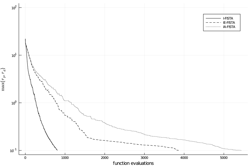
Figure 1: Convergence plot for the I-FISTA, IE-FISTA, and IA-FISTA methods on the $n=400$ and $\gamma=0.5$ test instance.

$n$	$\gamma$	I-FISTA			IE-FISTA			IA-FISTA
		$k$	fgs	time	$k$	fgs	time	$k$	fgs	time
100	0.10	27	45	0.1	35	155	0.3	26	52	0.1
	0.20	56	102	0.2	70	229	0.4	53	160	0.4
	0.30	88	169	0.4	111	360	0.6	85	330	0.7
	0.40	131	261	0.4	164	600	1.1	127	624	1.3
	0.50	130	269	0.4	162	617	1.1	125	676	1.3
	0.60	141	296	0.5	176	709	1.2	137	784	1.4
	0.70	143	300	0.5	178	827	1.4	139	817	1.4
	0.80	144	304	1.1	175	860	2.1	140	857	2.7
	0.90	147	310	0.6	179	871	1.9	142	887	1.8
	1.00	148	320	1.0	179	729	2.2	143	922	2.6
200	0.10	73	129	0.9	93	234	1.5	71	211	1.3
	0.20	170	333	2.0	211	692	3.9	165	738	4.3
	0.30	242	462	2.5	292	1099	5.9	235	1533	8.1
	0.40	248	475	2.5	306	1201	6.3	239	1508	8.0
	0.50	252	478	2.6	307	1165	6.1	243	1741	9.2
	0.60	251	477	2.8	309	1207	6.5	244	1738	9.3
	0.70	260	498	2.7	311	1122	6.0	250	1816	9.8
	0.80	266	505	2.8	322	1422	7.5	257	1977	10.6
	0.90	271	512	2.6	322	1711	8.9	260	1813	9.6
	1.00	273	520	2.7	327	1638	8.5	263	2044	10.7
300	0.10	124	241	2.9	147	403	5.1	121	414	5.4
	0.20	330	620	7.6	369	1421	17.5	312	2104	25.4
	0.30	332	621	7.7	383	1573	19.6	322	2699	34.4
	0.40	347	662	8.1	395	1447	17.8	335	3127	38.3
	0.50	355	640	8.1	405	1825	23.3	343	3136	39.3
	0.60	366	644	8.1	419	2858	36.4	355	3361	41.5
	0.70	371	648	8.0	423	3674	45.5	359	4013	48.8
	0.80	376	685	8.7	427	3672	46.7	364	4156	52.2
	0.90	380	703	8.8	430	4022	51.6	366	4855	59.7
	1.00	388	734	9.3	432	4223	53.7	373	4742	59.3
400	0.10	182	333	7.6	233	450	10.5	177	737	17.1
	0.20	413	783	17.4	511	2050	45.9	401	3829	82.2
	0.30	431	778	17.4	531	1790	40.1	418	5430	118.4
	0.40	450	803	18.4	549	2503	56.1	436	5147	111.8
	0.50	467	806	18.0	567	3715	83.9	453	5440	118.1
	0.60	479	881	19.7	578	4632	103.9	462	5828	126.8
	0.70	489	919	20.6	585	4075	91.3	472	6439	140.8
	0.80	499	945	21.2	596	3701	83.3	480	6974	153.2
	0.90	507	947	21.3	602	3944	89.1	488	7543	165.1
	1.00	509	971	22.2	611	3459	78.8	491	7490	166.2

Table 1: The number of iterations ($k$), function/gradient evaluations (fgs), and time in seconds for the I-FISTA, IE-FISTA, and IA-FISTA methods for $n=100,200,300,400$.

$n$	$\gamma$	I-FISTA			IE-FISTA			IA-FISTA
		$k$	fgs	time	$k$	fgs	time	$k$	fgs	time
500	0.10	265	513	20.2	320	667	26.3	257	1203	45.8
	0.20	499	934	35.0	595	2429	94.6	484	5940	216.7
	0.30	529	924	35.3	626	2716	102.8	513	7012	261.6
	0.40	559	994	37.4	654	5697	214.6	539	9331	340.8
	0.50	573	1072	40.5	669	4672	175.9	553	7133	260.5
	0.60	591	1117	42.4	679	4781	182.3	569	7549	279.0
	0.70	598	1093	41.5	700	6730	256.2	578	7455	275.4
	0.80	607	1173	44.5	705	5664	215.5	585	8618	318.7
	0.90	617	1146	43.6	711	4724	180.1	594	8562	318.1
	1.00	626	1227	46.7	721	3796	144.9	604	9962	369.4
600	0.10	377	709	46.6	434	1102	72.0	366	2919	185.3
	0.20	586	1085	68.4	678	3109	194.5	567	9471	576.4
	0.30	629	1089	67.2	723	4896	303.7	610	8744	525.9
	0.40	662	1132	66.8	750	6461	383.7	636	9164	526.4
	0.50	683	1263	76.1	777	5335	318.3	660	10852	629.3
	0.60	696	1282	78.5	792	5446	332.7	673	12647	751.9
	0.70	710	1333	82.5	801	7079	439.5	685	12607	758.0
	0.80	729	1368	82.9	811	5087	307.4	703	9818	576.0
	0.90	733	1388	84.3	832	4203	257.1	708	10843	640.3
	1.00	739	1439	89.0	840	5726	354.7	715	10698	645.6
700	0.10	521	979	89.4	586	1859	169.5	498	6468	571.7
	0.20	673	1251	109.0	762	3394	298.6	651	10581	896.6
	0.30	725	1217	105.7	819	6842	596.5	703	12948	1094.2
	0.40	762	1424	124.1	847	5549	485.3	733	11215	951.6
	0.50	786	1380	121.6	871	6919	606.9	756	11574	987.7
	0.60	803	1524	135.3	888	7032	626.5	773	13455	1160.8
	0.70	819	1511	133.9	911	8809	783.1	791	15117	1301.1
	0.80	828	1540	137.7	923	8837	792.4	800	15366	1335.4
	0.90	842	1624	142.8	932	9432	829.4	813	15936	1369.9
	1.00	855	1661	148.7	941	9716	873.2	824	17285	1509.8
800	0.10	692	1286	165.3	756	3108	400.4	670	11408	1420.6
	0.20	762	1421	177.2	848	3697	454.4	738	14087	1682.3
	0.30	822	1347	173.1	907	6835	878.1	794	12437	1542.9
	0.40	862	1573	199.0	947	7783	995.7	832	14689	2041.1
	0.50	887	1639	208.1	970	7028	893.4	856	16092	1985.1
	0.60	910	1700	213.7	995	9012	1131.0	879	18385	2242.0
	0.70	923	1747	225.2	1013	9210	1188.9	892	18666	2296.6
	0.80	943	1805	231.3	1023	8011	1032.9	905	13242	1651.0
	0.90	960	1840	238.7	1036	10180	1324.2	927	14950	1892.3
	1.00	971	1884	243.9	1056	11607	1502.1	937	16054	2026.2

Table 2: The number of iterations ($k$), function/gradient evaluations (fgs), and time in seconds for the I-FISTA, IE-FISTA, and IA-FISTA methods for $n=500,600,700,800$.

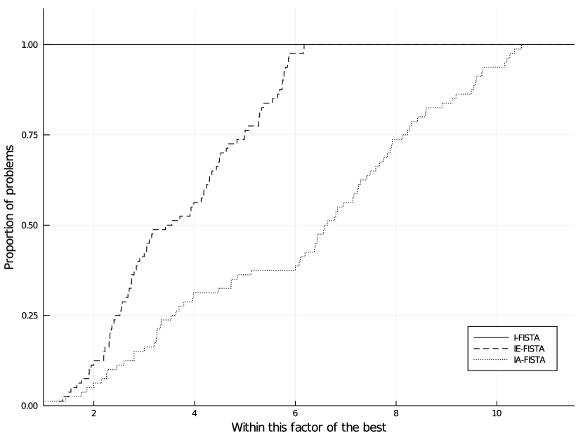
Figure 2: Performance profile of total running time for the I-FISTA, IE-FISTA, and IA-FISTA methods on all test instances.

An example of the typical convergence behavior of the three methods is shown in Fig. 1 where the value of $\max\{r_{p},r_{d}\}$ is plotted each time $\phi(y)$ and $\nabla\phi(y)$ are evaluated. Note, however, that during the linesearch procedure of L-BFGS-B, the value of $\max\{r_{p},r_{d}\}$ may vary drastically, so, to obtain a plot without such noise, we replace those intermediate linesearch values with the value obtained at the termination of the linesearch or when the stopping condition for the subproblem is satisfied.

In Tables 1 and 2 we record the number of outer iterations ($k$), the number of function/gradient evaluations (fgs), and the total running time in seconds, but not including the time to compute the initial point. From these results, it is clear that $k$, fgs, and time increase for all three methods as $n$ increases and as $\gamma$ increases. However, we also see that although I-FISTA and IE-FISTA require more outer iterations than IA-FISTA, each require fewer total inner iterations (i.e., fgs), and hence less time, than IA-FISTA to solve each instance to the desired tolerance.

Here we include an interesting point. In our numerical tests we observed that L-BFGS-B was always able to satisfy the IR Rule, typically in a small number of iterations. However, we were curious to see that sometimes L-BFGS-B failed to satisfy the IER Rule and only stopped due to a failure of the linesearch or due to having identical function values on two consecutive function evaluations. We would like to investigate this behavior in greater detail in future research.

To see the forest for the trees, in Fig. 2 we plot the performance profile [16, 17, 24] of the numerical results from Tables 1 and 2 using the total running time of each solver on each instance. From this plot we clearly see that I-FISTA is the fastest on all test instances and that IE-FISTA also outperforms IA-FISTA on the test instances. Thus, although all three algorithms have the same theoretical rate of convergence, we have demonstrated that the relative error rules and corresponding algorithms proposed in this paper, I-FISTA and, to a lesser extent, IE-FISTA, are potentially valuable to use in situations where IA-FISTA has proved successful in practice.

7 Final Remarks

This paper proposed and analyzed two inexact versions of FISTA for minimizing the sum of two convex functions. Both schemes allow their subproblems to be solved inexactly subject to satisfying certain relative error rules. Numerical experiments were carried out in order to illustrate the numerical behavior of the methods. They indicate that the proposed methods based on inexact relative error rules are more efficient than those based on the inexact absolute error rule on a set of instances of the $H$-weighted nearest correlation matrix problem.

References

• [1] E. Anderson, Z. Bai, C. Bischof, S. Blackford, J. Demmel, J. Dongarra, J. Du Croz, A. Greenbaum, S. Hammarling, A. McKenney, and D. Sorensen, LAPACK Users’ Guide, Society for Industrial and Applied Mathematics, Philadelphia, PA, third ed., 1999.
• [2] H. Attouch and A. Cabot, Convergence rates of inertial forward-backward algorithms, SIAM J. Optim., 28 (2018), pp. 849--874.
• [3] H. Attouch, A. Cabot, Z. Chbani, and H. Riahi, Inertial forward-backward algorithms with perturbations: application to Tikhonov regularization, J. Optim. Theory Appl., 179 (2018), pp. 1--36.
• [4] H. Attouch, Z. Chbani, J. Peypouquet, and P. Redont, Fast convergence of inertial dynamics and algorithms with asymptotic vanishing viscosity, Math. Program., 168 (2018), pp. 123--175.
• [5] H. Attouch and J. Peypouquet, The rate of convergence of Nesterov’s accelerated forward-backward method is actually faster than $1/k^{2}$, SIAM J. Optim., 26 (2016), pp. 1824--1834.
• [6] J.-F. Aujol and C. Dossal, Stability of over-relaxations for the forward-backward algorithm, application to FISTA, SIAM J. Optim., 25 (2015), pp. 2408--2433.
• [7] H. H. Bauschke, M. Bui, and X. Wang, Applying FISTA to optimization problems (with or) without minimizers, Mathematical Programming, 192 (2019), pp. 1--20.
• [8] A. Beck and M. Teboulle, A fast iterative shrinkage-thresholding algorithm for linear inverse problems, SIAM Journal on Imaging Sciences, 2 (2009), pp. 183--202.
• [9] A. Beck and M. Teboulle, Gradient-based algorithms with applications to signal-recovery problems, in Convex optimization in signal processing and communications, Cambridge Univ. Press, Cambridge, 2010, pp. 42--88.
• [10] J. Y. Bello Cruz, On proximal subgradient splitting method for minimizing the sum of two nonsmooth convex functions, Set-Valued and Variational Analysis, 25 (2017), pp. 245--263.
• [11] J. Y. Bello Cruz, G. Li, and T. T. A. Nghia, On the $Q$-linear convergence of forward-backward splitting method and uniqueness of optimal solution to Lasso, 2018, arXiv:1806.06333.
• [12] J. Y. Bello Cruz and T. A. Nghia, On the convergence of the forward--backward splitting method with linesearches, Optim. Methods Softw., 31 (2016), pp. 1209--1238.
• [13] J. Bezanson, A. Edelman, S. Karpinski, and V. Shah, Julia: A fresh approach to numerical computing, SIAM Review, 59 (2017), pp. 65--98.
• [14] R. Borsdorf and N. J. Higham, A preconditioned Newton algorithm for the nearest correlation matrix, IMA Journal of Numerical Analysis, 30 (2010), pp. 94--107.
• [15] A. Chambolle and C. Dossal, On the convergence of the iterates of the ‘‘fast iterative shrinkage/thresholding algorithm’’, J. Optim. Theory Appl., 166 (2015), pp. 968--982.
• [16] E. D. Dolan and J. J. Moré, Benchmarking optimization software with performance profiles, Mathematical Programming, 91 (2002), pp. 201--213.
• [17] N. Gould and J. Scott, A note on performance profiles for benchmarking software, ACM Trans. Math. Softw., 43 (2016).
• [18] E. T. Hale, W. Yin, and Y. Zhang, Fixed-point continuation for $l_{1}$-minimization: methodology and convergence, SIAM J. Optim., 19 (2008), pp. 1107--1130.
• [19] K. Jiang, D. Sun, and K.-C. Toh, An inexact accelerated proximal gradient method for large scale linearly constrained convex SDP, SIAM J. Optim., 22 (2012), pp. 1042--1064.
• [20] D. Lewandowski, D. Kurowicka, and H. Joe, Generating random correlation matrices based on vines and extended onion method, Journal of Multivariate Analysis, 100 (2009), pp. 1989 -- 2001.
• [21] R. D. C. Monteiro and B. F. Svaiter, On the complexity of the hybrid proximal extragradient method for the iterates and the ergodic mean, SIAM Journal on Optimization, 20 (2010), pp. 2755--2787.
• [22] R. D. C. Monteiro and B. F. Svaiter, An accelerated hybrid proximal extragradient method for convex optimization and its implications to second-order methods, SIAM Journal on Optimization, 23 (2013), pp. 1092--1125.
• [23] J. L. Morales and J. Nocedal, Remark on ‘‘Algorithm 778: L-BFGS-B: Fortran subroutines for large-scale bound constrained optimization’’, ACM Trans. Math. Softw., 38 (2011), pp. 1--4.
• [24] J. J. Moré and S. M. Wild, Benchmarking derivative-free optimization algorithms, SIAM Journal on Optimization, 20 (2009), pp. 172--191.
• [25] Y. Nesterov, A method for solving the convex programming problem with convergence rate $O(1/k^{2})$, Dokl. Akad. Nauk SSSR, 269 (1983), pp. 543--547.
• [26] Y. Nesterov, An approach to constructing optimal methods for minimization of smooth convex functions, Èkonom. i Mat. Metody, 24 (1988), pp. 509--517.
• [27] Y. Nesterov, Smooth minimization of non-smooth functions, Math. Program., 103 (2005), pp. 127--152.
• [28] Y. Nesterov, Gradient methods for minimizing composite functions, Mathematical Programming, 140 (2013), pp. 125--161.
• [29] H. Qi and D. Sun, A quadratically convergent Newton method for computing the nearest correlation matrix, SIAM J. Matrix Anal. Appl., 28 (2006), pp. 360--385.
• [30] H. Qi, D. Sun, and Y. Gao, CorNewton3.m: A Matlab code for computing the nearest correlation matrix with fixed diagonal and off diagonal elements. https://www.polyu.edu.hk/ama/profile/dfsun/CorNewton3.m, 2009.
• [31] M. V. Solodov and B. F. Svaiter, A hybrid approximate extragradient-proximal point algorithm using the enlargement of a maximal monotone operator, Set-Valued Anal., 7 (1999), pp. 323--345.
• [32] W. Su, S. Boyd, and E. J. Candès, A differential equation for modeling Nesterov’s accelerated gradient method: theory and insights, J. Mach. Learn. Res., 17 (2016), pp. Paper No. 153, 43.
• [33] J. A. Tropp, Just relax: convex programming methods for identifying sparse signals in noise, IEEE Trans. Inform. Theory, 52 (2006), pp. 1030--1051.
• [34] S. Villa, S. Salzo, L. Baldassarre, and A. Verri, Accelerated and inexact forward-backward algorithms, SIAM J. Optim., 23 (2013), pp. 1607--1633.
• [35] C. Zhu, R. H. Byrd, P. Lu, and J. Nocedal, Algorithm 778: L-BFGS-B: Fortran subroutines for large-scale bound-constrained optimization, ACM Trans. Math. Softw., 23 (1997), pp. 550--560.