Opportunistic Intermittent Control with Safety Guarantees
for Autonomous Systems

Abstract

Control schemes for autonomous systems are often designed in a way that anticipates the worst case in any situation. At runtime, however, there could exist opportunities to leverage the characteristics of specific environment and operation context for more efficient control. In this work, we develop an online intermittent-control framework that combines formal verification with model-based optimization and deep reinforcement learning to opportunistically skip certain control computation and actuation to save actuation energy and computational resources without compromising system safety. Experiments on an adaptive cruise control system demonstrate that our approach can achieve significant energy and computation savings.

I Introduction

For safety-critical autonomous systems such as robots and automated vehicles, control schemes are often designed conservatively so that system safety can be maintained in a wide variety of situations [1, 2, 3]. During the operation of these systems, however, such schemes can be overly conservative and result in unnecessary resource and/or energy consumption. This paper first makes the observation that certain control steps, even if they are skipped, do not impact either the performance or safety of the overall system. Armed with this observation, we propose an online scheme that opportunistically skips control computation and the corresponding actuation steps by learning specific characteristics of the system’s operating environment. We further show that safety could be maintained with this more efficient control scheme.

Consider the example of an adaptive cruise control (ACC) system, in which an ego vehicle automatically adjusts its speed to maintain a safe distance from the vehicle in front. To ensure the safety across a variety of situations (e.g. an aggressive front vehicle vs. a conservative front vehicle), the ego vehicle may adopt a safe control scheme such as one that based on robust model predictive control (RMPC) [1]. At each control step, the RMPC calculates the actuation signal based on the two vehicles’ speeds and their relative distance. However, it does not make any prediction on the front vehicle’s intent. In practical scenarios, the front vehicle may exhibit certain behavior patterns, e.g., an aggressive driver that accelerates and decelerates frequently, or stop-and-go in a traffic jam. We argue that we can design more computation/energy-efficient control schemes by learning and exploiting these patterns. The key is how to learn these patterns quickly and how to guarantee system safety when certain control steps are skipped.

In this work, we consider systems with an existing safe controller, and develop a novel online intermittent-control framework to opportunistically skip the computation and actuation of the underlying controller by leveraging the characteristics of specific operation context and environment. For instance, at each control step of the above ACC example, our method will decide whether to run the underlying RMPC and apply its actuation/control input, or simply apply a zero control input. Such opportunistic skipping could help save computational resources for running the underlying control algorithm and save actuation energy by applying zero control inputs. To achieve both safety and efficiency, our method addresses two key challenges: 1) How to ensure the system safety when zero input is applied at some control steps? 2) How to effectively leverage the characteristics of specific operation context and environment?

For the first challenge, our framework uses formal analysis to guarantee the system safety under skipping of controls. Specifically, we first compute a strengthened safe set based on the notion of robust control invariant and backward reachable set of the underlying safe controller. Intuitively, the strengthened safety set represents the states at which the system can accept any control input at the current step and be able to stay within safe states, with the underlying safe controller applying input from the next step on. We then develop a monitor to check whether the system is within such strengthened safe set at each control step. Whenever it is found that the system state is out of the strengthened safe set, the monitor will require the system to apply the underlying safe controller for guaranteeing system safety.

For the second challenge, we develop two approaches to leverage the characteristics of operation context and environment when the system is within the strengthened safe set, depending on the type of the underlying safe controller and whether the characteristics are known explicitly. In the simpler case where the safe controller has an analytic expression and the characteristics can be explicitly captured, we use a model-based approach to decide the skipping choices by solving a mixed integer programming (MIP) program. Otherwise, we use a deep reinforcement learning (DRL) approach to learn the mapping from the current state and the historical characteristics to the skipping choices, which implicitly reflects the impact of specific operation context and environment.

Related work: Our work is related to the rich literature on weakly-hard systems and fault-tolerant control systems. In weakly-hard systems, occasional deadline misses are allowed for control computation in a bounded manner, e.g., the typical $(m,K)$ constraint allows at most $m$ deadline misses in any $K$ consecutive control instances [4, 5, 6]. In fault-tolerant control systems, broader fault types (e.g., sensing, actuation, or system errors) and fault models (e.g., stochastic model) are considered [7]. However, while these works try to preserve the system safety [8, 9, 10] or stability [11, 12] under passive faults, our work considers skipping control operations proactively to save resources for control computation and reduce energy for actuation.

Our work is also related to methods on safe reinforcement learning [13, 14, 15], as we also restrict the possible system actions to a safe set for ensuring safety. The difference is that our approach computes the safe action set by deriving the robust control invariant and backward reachable set of an underlying controller and then leverages the safe set for proactively exploring control skippings.

In summary, this work makes the following novel contributions.

• We develop a novel online intermittent-control framework for opportunistically skipping the computation and actuation of an underlying safe controller to save computational resources and actuation energy. Our framework can be generally applied to various underlying controllers in a discrete linear time-invariant system, and achieves both safety and efficiency.

• Our framework ensures safety by developing a formal method to compute a strengthened safe set of the underlying controller.

• Our framework achieves efficiency by developing a model-based approach and a DRL-based approach to decide the skipping choices of the underlying controller under different scenarios. The model-based approach is applied when the underlying controller has an analytic expression and the characteristics of specific operation context and environment are explicitly known; while the DRL approach is applied otherwise.

• We demonstrate the effectiveness of our approach through extensive experiments on an ACC case study, using the widely-used SUMO (Simulation of Urban Mobility) simulator [16].

II Problem Formulation

We consider a discrete linear time-invariant (LTI) system described by the following difference equation:

$$x(t+1)=Ax(t)+Bu(t)+w(t),\qquad t\geq 0,$$ (1)

where $x\in\mathcal{R}^{n}$ is the state variable, $u\in\mathcal{R}^{m}$ is the control input variable, and $w$ is a bounded perturbation. $A$ and $B$ are transformation matrix. We assume that the state space of the system is $\mathcal{R}^{n}$. The constraints on the safe state, the control input, and the bounded perturbation are

$$x(t)\in X,\qquad u(t)\in U,\qquad w(t)\in W,$$ (2)

where $X\subset\mathcal{R}^{n}$, $U\subset\mathcal{R}^{m}$ and $W\subset\mathcal{R}^{k}$ are polytopes, and $0\in X$, $0\in U$, $0\in W$. Note that $X$ represents the set of safe states, and perturbation $w(t)$ captures the characteristics of the specific operation context and environment.

We assume that such system can be controlled by a safe feedback controller $\kappa$. At each sampling instant $t=0,1,\cdots$, the system reads the state $x(t)$ of the plant and feeds it to the controller $\kappa$ to obtain the control input $u=\kappa(x)$. The new input $u(t)$ will be applied at the next time step. We use 1-norm of the input $\|u(t)\|_{1}$ to represent the energy cost at each control step.

A well-designed controller $\kappa$ may ensure the system safety by sustaining any possible perturbation. However, when applying in practice, such design may be over-conservative and energy-consuming. Thus, the question is whether we can save actuation energy (and possibly also computational resources) by skipping the computation and actuation of control inputs (i.e. using zero inputs) at some steps. This requires effectively leveraging the dynamic characteristics of specific operation context and environment at runtime (reflected via the pattern of perturbation $w(t)$), while guaranteeing system safety.

We use a binary indicator $z(t)$ at time step $t$ to represent the skipping choice: $1$ denotes actuating the control input computed by the controller $\kappa$, and $0$ denotes skipping the control and applying zero input. Our online opportunistic intermittent-control problem can be formulated as follows.

Problem 1 (Online Opportunistic Intermittent-Control Problem).

Given a dynamical system defined in Equation (1) and a controller $\kappa$ that can ensure system safety, i.e., $x(t)\in X$, the opportunistic intermittent-control problem is to determine the skipping choice variable $z(t)$ at each control instant $t$, such that the system will stay within $X$ and the overall energy cost $\sum_{i=0}^{\infty}\|u(t)\|$ is minimized.

III Opportunistic Intermittent-Control Framework

There are two key aspects of our approach: 1) ensuring that the system always stays within the safe state space $X$, and 2) deciding the skipping choice variable $z(t)$ by leveraging the characteristics of perturbation $w$.

For the first aspect, to ensure system safety, we define three safe state sets of different levels, namely the original safe set $X$, the robust invariant set $X_{I}$, and the strengthened safe set $X^{\prime}$, as shown in Figure 1. The original safe set $X$ is the largest of the three, and given by the problem definition. While the system is still safe within this set, there is no guarantee that it will stay within $X$ for the next time step, even with the input from the underlying safe controller $\kappa$. Thus, we consider the robust invariant set $X_{I}\subseteq X$. When the system is within this set, it is still controllable and can remain in this set by applying the controller $\kappa$. Finally, for considering skipping controls, we define the strengthened safe set $X^{\prime}\subseteq X_{I}$. When the system is within this set, it will stay within $X_{I}$ (and thus controllable and safe) for the next time step, regardless of the skipping choice at the current step (i.e., regardless of whether $z(t)$ is $1$ or $0$). Intuitively, the goal of our framework is to make skipping choices when the system is within the strengthened safe set $X^{\prime}$, and to apply the underlying safe controller $\kappa$ whenever the system goes out of $X^{\prime}$ but is still within the robust invariant set $X_{I}$ ($\kappa$ will be applied until the system goes back to $X^{\prime}$). Note that the system is guaranteed to never go out of $X_{I}$ and thus maintain safety.

Figure 1: Three safe state sets of different levels: strengthened safe set $X^{\prime}$, robust invariant set $X_{I}$, and original safe set $X$. For instance, for $x_{1}\in X^{\prime}$, in the next time step the system may steer to either $x_{2}$ or $x_{3}$ that are both within $X_{I}$ and hence safe and controllable. For $x_{3}\in X_{I}-X^{\prime}$, the system may steer to $x_{4}$ in the next step by applying actuation from $\kappa$, which is still controllable. However, if applying zero input at $x_{3}$, the system may go out of $X_{I}$ and steer to $x_{5}\in X-X_{I}$. $x_{5}$ is a safe state for now. However there is no guarantee that the system will remain within $X$ in the next step, even with the actuation from $\kappa$.

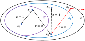
For the second aspect of our approach, to decide the skipping choices, we develop a model-based approach and a DRL-based approach for different scenarios based on whether the underlying controller has an analytic form and whether the characteristics of the perturbation $w(t)$ is known.

Figure 2: Schematic of our online opportunistic intermittent-control framework. Note that at time step $t-1$ and $t+2$, the system state is in the strengthened safe set $X^{\prime}$, and thus the skipping choice variable can be freely chosen.

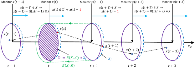
The schematic of our opportunistic intermittent-control framework is shown in Figure 2. Its flow is shown in Algorithm 1. As aforementioned, to ensure safety, we will first compute the robust invariant set $X_{I}$ and the strengthened safe set $X^{\prime}$ (lines 1). In our approach, the initial state has to be within $X_{I}$ (line 2). During operation, at each time step $t$, we will monitor the current state $x(t)$ by collecting sensor inputs. If $x(t)$ is within $X^{\prime}$, we know that the system will remain within $X_{I}$ regardless of whether we skip the actuation from $\kappa$ at this step, and we will determine the skipping choice $z(t)$ via a function $\Omega$ that uses the model-based approach or the DRL-based approach (line 6). If $x(t)$ is out of $X^{\prime}$ (i.e., within $X_{I}-X^{\prime}$), we cannot skip the actuation of $\kappa$ and have to set the skipping choice $z(t)$ to $1$ (line 9). Finally, depending on the value of $z(t)$, either the actuation input from $\kappa$ or zero input will be applied (lines 10 to 15).

1 Compute robust invariant set $X_{I}$ and strengthened safe set $X^{\prime}$;

2 Initialization: $t\leftarrow 0$, $x(0)\in X_{I}$;

3 while true do

4       Monitor the current state $x(t)$ via sensor inputs;

5       if $x(t)\in X^{\prime}$ then

6             $z(t)\leftarrow\Omega(x(t),\bar{w}(t))$;

7            

8      else

9             $z(t)\leftarrow 1$;

10            

11       end if

12      if $z(t)=1$ then

13             $u(t)\leftarrow\kappa(x(t))$;

14            

15      else

16             $u(t)\leftarrow 0$;

17            

18       end if

19      Actuate the control input $u(t)$;

20       $t\leftarrow t+1$;

21      

22 end while

Algorithm 1 Opportunistic Intermittent-Control Framework

The key components in our framework is the computation of $X_{I}$ and $X^{\prime}$ for ensuring safety, and the design of the function $\Omega$ for making skipping decisions. Next, we will introduce their details.

III-A Ensuring Safety: Computation of Robust Invariant Set $X_{I}$ and Strengthened Safe Set $X^{\prime}$

To compute $X_{I}$ and $X^{\prime}$, we first introduce the concept of robust control invariant set [17] and backward reachable set [18].

Definition 1 (Robust Control Invariant Set).

Given a discrete dynamical system as defined in Equation (1) and a controller $\kappa$, the robust control invariant set of the system is defined as:

$$X_{I}=\{x\ |\ \forall w\in W,x\in X_{I},\exists x^{\prime}\in X_{I},f(x,\kappa(x),w)=x^{\prime}\}.$$ (3)

Definition 2 (Backward Reachable Set).

Given a discrete dynamical system as defined in Equation (1), a controller $\kappa$ and a set $Y$, the (one-step) robust backward reachable set of the system from $Y$ under a skipping choice variable $z$ is defined as:

$$B(Y,z)=\begin{cases}\{x\ |\ \forall w\in W,x^{\prime}\in Y,f(x,\kappa(x),w)=x^{\prime}\},&z=1,\\ \{x\ |\ \forall w\in W,x^{\prime}\in Y,f(x,0,w)=x^{\prime}\},&z=0.\end{cases}$$

Definition 3 (Strengthened Safety Set).

Based on Definitions 3 and 2, we define the strengthened safe set $X^{\prime}$ as:

$$X^{\prime}=B(X_{I},0)\cap X_{I}.$$ (4)

Theorem 1 (Safety of Our Approach).

Let $X^{\prime}$ and $X_{I}$ be defined as Equation (4) and Equation (3), respectively, our framework can ensure the system safety for any skipping decision function $\Omega$.

Proof.

Since $X^{\prime}=B(X_{I},0)\cap X_{I}\subset X$, the system is safe if $x\in X^{\prime}$. Assume that at time step $t$, the monitor observes that the system goes out of the region $X^{\prime}$, i.e. $x(t)\in X_{I}-X^{\prime}$ (see Figure 2). While at the last time step $t-1$, the system was still in $X^{\prime}$, i.e. $x(t-1)\in X^{\prime}=B(X_{I},0)\cap X_{I}=B(X_{I},0)\cap B(X_{I},1)$. By the definition of backward reachable set, we know that $x(t)\in X_{I}$. Thus, based on the definition of robust controlled invariant, the system is controllable and will remain in $X_{I}$ under $\kappa$. This shows that our framework (Algorithm 1) will always maintain system safety. ∎

Computing $X_{I}$ and $X^{\prime}$. We first consider the computation of the robust control invariant set $X_{I}$. For linear feedback control, namely $\kappa(x)=Kx$, the robust invariant can be computed as [19]:

$$X_{I}=\alpha(W\oplus(A+BK)W\oplus\cdots\oplus(A+BK)^{n}W),$$

where $\alpha$ and $n$ ares hyper-parameters. $\oplus$ denotes the Minkowski sum.

For more advanced control algorithms, we take robust model predictive control (RMPC) as an example, which considers the nominal system model and tightened constraints [1, 2]. Given a system state $x(t)$, RMPC solves the following optimization:

$$\quad J(x(t))\triangleq\min_{\bar{u}_{N}}\sum_{k=0}^{N-1}P\|x(k|t)\|_{1}+Q\|u(k|t)\|_{1}$$ (5)

s.t. $$\begin{cases}x(k+1|t)=Ax(k|t)+Bu(k|t),\quad 0{\leq}k{\leq}N{-}1,\\ x(k|t)\in X(k),\quad 0{\leq}k{\leq}N,\\ u(k|t)\in U,\quad 0{\leq}k{\leq}N{-}1,\\ x(0|t)=x(t),\quad x(N|t)\in X_{t},\end{cases}$$

where $u(k|t)$ and $x(k|t)$ denote the input and state of $t+k$ predicted at $t$ respectively. $\bar{u}_{H}=u(0|t),\cdots,u(N-1|t)$, $P$ and $Q$ are the weights of the state cost and energy cost, respectively. $X_{t}$ is the terminate set to ensure stability [20], and the tightened constraints $X(k)$ is defined recursively as follows.

$$\begin{gathered}X(0)=X,\\ X(k)=\{x\ |\ x\in X(k{-}1)\ \wedge\ x\oplus A^{k-1}W\subseteq X(k{-}1)\},\ \ k\geq 1.\end{gathered}$$

Let $\bar{u}^{*}_{N}$ be the optimal solution. Then the first sample of $\bar{u}^{*}_{N}$ will be applied for actuation: $\kappa(x(t))=u^{*}(0|t)$. We leverage the idea of explicit MPC [21] to first analyze the feasible region of MPC, namely, the state set where MPC optimization is feasible. Assuming the feasible set of the given RMPC is $X_{F}$, we have:

Proposition 1.

The feasible set $X_{F}$ of the RMPC is also its robust control invariant set (i.e., $X_{I}=X_{F}$), if the terminal set $X_{t}$ ensures stability, that is, there exists a robust local controller $\kappa_{L}$ such that $\kappa_{L}(x)+w\in X_{T}$, $\forall x\in X_{T},w\in W$.

Proof.

Given any $x(t)\in X_{F}$, by the definition of $X_{F}$, we know that the optimization problem of $J(x(t))$ is feasible and let the optimal solution be $\bar{u}^{*}_{N}$. We also let the corresponding optimal value of $x(1|t),\cdots,x(N|t)$ be $x^{*}(1|t),\cdots,x^{*}(N|t)$. By the methodology of MPC, we know that the system will steer to $x(t+1)=x^{*}(1|t)+w(t)\in X(0)$. Now we consider the feasibility of the optimization problem $J(x(t+1))$. We construct a control sequence by combining part of the optimal value of $\bar{u}^{*}_{N}$ and the local controller $\kappa_{L}$, namely $u^{*}(1|t),\cdots,u^{*}(N-1|t),\kappa_{L}(x^{*}(N|t))$. We have This control sequence is feasible for $J(x(t+1))$. Therefore we have $x^{*}(1|t){\in}X_{F}$, which means $X_{F}$ is the robust control invariant set. ∎

After obtaining the robust control invariant $X_{I}$ for the RMPC, we can compute the backward reachable set $B(X_{I},0)$ using the following formula if $A$ is invertible:

$$B(X_{I},0)=A^{-1}(X_{I}\ominus W),$$

where $\ominus$ denotes the Minkowski difference.

III-B Achieving Efficiency: Design of Skipping Decision Function $\Omega$

As aforementioned, we develop a model-based approach and a DRL-based approach for making the skipping decisions (function $\Omega$ in Algorithm 1), with the system safety guaranteed by Theorem 1.

III-B1 Model-based Approach

If the control law can be represented as an analytic expression and the perturbation is known, i.e. $w(t)$ is known for any $t\geq 0$, we can develop a model-based approach for optimizing the skipping choice made in function $\Omega$. Specifically, at each time step $t$, we solve the following finite-time optimization problem:

$$\qquad\qquad\min_{\bar{z}_{H},\bar{u}_{H},\bar{x}_{H}}\sum_{k=0}^{H-1}\|u(k|t)\|_{1}$$ (6)

s.t. $$\begin{cases}x(k+1|t){=}f(x(k|t),u(k|t),w(k|t)),\ 0{\leq}k{\leq}H{-}1,\\ x(k+1|t)\in X^{\prime},\ \ u(k|t)\in U,\quad 0{\leq}k{\leq}H{-}1,\\ u(k)\in\begin{cases}\kappa(x(k)),&z(t)=1,\\ 0,&z(t)=0.\end{cases}\quad 0{\leq}k{\leq}H{-}1,\\ x(0|t)=x(t),\end{cases}$$

where $\bar{z}_{H}=z(0|t),\cdots,z(H-1|N)$, $\bar{u}_{H}=u(0|t),\cdots,u(H-1|N)$, and $\bar{x}_{H}=x(0|t),\cdots,x(H|N)$. Let $\bar{z}^{*}_{H}$ be the optimal solution. Then the first sample of $\bar{z}^{*}_{H}$ will be applied as the skipping decision, i.e., $\Omega(x(t))=z^{*}(0|t)$.

Remark 1.

The above optimization formulation (6) is in fact similar to MPC [22], as it is also based on the idea of deciding present action by predicting long-term behavior. However, note that our optimization does not encode terminal constraint as in [20] as stability does not need to be considered.

III-B2 DRL-based Approach

Most advanced control schemes such as the MPC cannot be simply represented as an analytic expression. Furthermore, it is often impossible to know the perturbation $w(t)$ that reflects the specific operation context and environment a prior. In such case, we develop a machine learning approach for the skipping decision function $\Omega$ to learn and leverage the underlying perturbation pattern. Since there is typically a lack of labelled data for such systems in practice, we use a deep reinforcement learning (DRL) based approach rather than supervise learning. Specifically, we design the following DRL agent for $\Omega$.

Actions. The DRL agent generates two types of actions, $0$ or $1$, representing the cases of $z(t)=0$ or $z(t)=1$ in skipping decision.

State. The action of $\Omega$ depends on not only the observation of current system state, but also the information of past perturbations. Thus, we define a hyper-parameter $r$, which represents the memory length of the perturbations. The state for the DRL agent is the set as $s(t)=\{x(t),w(t-r+1),\cdots,w(t)\}$.

Reward (Penalty) function. Typically, if the system goes out of the strengthened safe set $X^{\prime}$ frequently, more non-zero inputs computed by the underlying controller $\kappa$ need to be applied and there is less energy saving. Thus, the goal of the DRL agent should include both minimizing the energy cost $\sum{\|u(t)\|_{1}}$ directly and maintaining the system within the strengthened safe set $X^{\prime}$. Following this idea, we design the reward function $R(s_{1},z,s_{2})$ of DRL with respect to the agent predecessor state $s_{1}$, the action $z$ and the successor state $x_{2}$, with consideration of both objectives:

$$\begin{gathered}R(s_{1},z,s_{2})=-w_{1}\cdot R_{1}-w_{2}\cdot R_{2},\\ R_{1}=\begin{cases}0,&x_{2}\in X^{\prime},\\ 1,&x_{2}\in{{X_{I}}-{X^{\prime}}},\end{cases}\ \ R_{2}=\begin{cases}0,&z{=}0\wedge x_{1}{\in}X^{\prime},\\ \|\kappa(x_{1})\|_{1},&others.\end{cases}\end{gathered}$$

where $R_{1}$ and $R_{2}$ are the reward for maintaining the system state $x$ in $X^{\prime}$ and the reward for the current energy cost, respectively. $w_{1}$ and $w_{2}$ are the weights for $R_{1}$ and $R_{2}$.

Learning process. Our DRL agent interacts with the underlying controller $\kappa$ at each time step. For convenience, we let $w(-r+1),\cdots,w(-1)$ be $0$. The DRL agent starts with the initial state $s(0)=\{x(0),w(-r+1),\cdots,w(0)\}$, and generates the first action $z(0)$. If $z(0)=1$ and $x_{1}{\in}X^{\prime}$, the underlying controller $\kappa$ will be applied to compute the control input $u(0)=\kappa(x(0))$; otherwise, we let $u(0)=0$. Once $u(0)$ is applied, the next system state $x(1)$ is generated. We can then calculate the reward and run the policy network based on the reward, and then obtain the action $z(1)$ for the next step. We repeat this until we reach the maximum steps, which is a hyper-parameter set in advance.

Note that when the DRL agent drives the system state out of the strengthened safe set $X^{\prime}$ (i.e., into $X_{I}-X^{\prime}$), we will apply the underlying controller $\kappa$ to ensure system safety. The DRL agent will also receive a large penalty in such case (as defined above in the reward function), so it can be motivated to keep the system state within $X^{\prime}$ for more efficient control and better learning of the perturbation pattern.

IV Experimental Results on an ACC Case Study

Figure 3: Schematic view of a cruise control scenario.

In our experiments, we conduct an extensive case study on an adaptive cruise control (ACC) system [9, 23]. As shown in Figure 3, there are two vehicles Ego and Front driving on the road. The Front vehicle is moving at a velocity $v_{f}$ (which may change over time). We are able to control the Ego vehicle by tuning its acceleration with a velocity-related resistance. Let $s$ be the relative distance between Ego and Front, and $v$ be the velocity of Ego. The system dynamics follow the standard Newton’s laws of motion:

$$\left\{\begin{array}[]{lcl}s(t+1)&=&s(t)-(v(t)-v_{f}(t))\delta,\\ v(t+1)&=&v(t)-(kv(t)-u(t))\delta,\end{array}\right.$$

where $(s,v)$ forms the state variable and $u$ is the control input variable. $\delta=0.1$ is the sampling/control period, and $k=0.2$ is the drag coefficient. The velocity of the Front vehicle is within the range $v_{f}\in[30,50]$. The ACC system tries to maintain the distance between the two vehicles within a safe range $s\in[120,180]$ for any possible $v_{f}$. The Ego vehicle has constraints on its velocity and actuation/control input: $v\in[25,55],u\in[-40,40]$. The control input $u$ is computed by the aforementioned RMPC $\kappa_{R}$ [1] with the prediction horizon set to $10$.

As mentioned in Section III, for an advanced controller as RMPC, we use double deep Q learning [24] to design the skipping decision function $\Omega$. The hyper-parameters used in DRL are set as follows. The perturbation memory length $r=1$. The weights in the reward function $w_{1}=0.01$ and $w_{2}=0.0001$. The training and testing of all the experiments are performed on a desktop with 4-core 3.60 GHz Intel Core i7 and NVIDIA GeForce GTX TITAN. The system is simulated in the SUMO simulator [16]. We evaluate the fuel consumption of $100$ time steps.

IV-A Overall Effectiveness of Our Approach

We compare our opportunistic intermittent-control approach against the traditional approach of only using the underlying RMPC controller, and against an intuitive bang-bang control scheme based on our framework. The bang-bang scheme uses the same computation of $X_{I}$ and $X^{\prime}$ in Section III-A to ensure system safety, but uses a simple strategy (instead of DRL) for deciding skipping choices. Specifically, it applies zero control input whenever the system state is within the strengthened safe set $X^{\prime}$, and applies the input from RMPC once it is not in $X_{I}-X^{\prime}$ :

$$u(x)=\begin{cases}0&x\in X^{\prime},\\ \kappa_{R}(x)&x\in X-X^{\prime}.\\ \end{cases}$$ (7)

In this experiment, we assume that the front vehicle is driving under a sinusoidal velocity variation pattern with a minor disturbance. Specifically,

$$v_{f}(t)=v_{e}+a_{f}sin(\frac{\pi}{2}\delta t)+w,$$ (8)

where $v_{e}=40$, $a_{f}=9$, and the random disturbance $w\in[-1,1]$. We conducted experiments on 500 cases with randomly generated initial state $x(0)$.

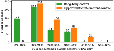
We first compare the fuel consumption of the three approaches (DRL-based opportunistic intermittent-control, bang-bang control, and RMPC only). The fuel consumption data are from SUMO simulations, and directly reflect the actuation energy cost as defined in our Problem 1. Figure 4 shows the fuel consumption savings of our DRL-based opportunistic intermittent-control approach and the bang-bang control approach over the traditional method of only using RMPC. The x-axis is the range of fuel consumption saving, and the y-axis shows how many cases (out of the 500) falls into each range for the two approaches. We can clearly see that 1) both the DRL-based opportunistic intermittent-control and the bang-bang control achieve significant savings, showing the potential of skipping controls when possible; 2) the DRL-based opportunistic intermittent-control achieves substantially more savings than the bang-bang control, showing the effectiveness of our DRL-based approach in learning the perturbation pattern and intelligently deciding the skipping choices. Overall, compared with RMPC, the average fuel consumption of bang-bang control is reduced by $16.28\%$, while the average fuel consumption of our DRL-based opportunistic intermittent-control is reduced by $23.83\%$.

Figure 4: Fuel consumption comparison on 500 test cases. X-axis shows the range of fuel consumption savings of our DRL-based opportunistic intermittent-control and bang-bang control over the traditional method of only using RMPC. The y-axis shows how many cases (out of the 500) falls into each range for the two approaches.

We also measured the computational savings from skipping the RMPC control computation. For our DRL-based opportunistic intermittent-control approach, the computation time for checking the satisfaction of strengthened safe set $X^{\prime}$ and invoking the neural network to decide skipping choice $z$ is in average 0.02 second; while the average computation time for RMPC is 0.12 second. In our experiments, out of 100 steps, the average number of steps that skip the RMPC computation is 79.4. Thus, overall, there is around $60\%$ saving in computation time from our approach (i.e., $(0.12\times 100-(0.02\times 100+0.12\times(100-79.4)))/(0.12\times 100)$).

IV-B Impact Analysis under Different Driving Scenarios

We further conducted a series of experiments to evaluate our approach under different driving scenarios, particularly when the Front vehicle exhibits different driving patterns. We are interested to see whether our approach can effectively learn those patterns and leverage them in achieving energy savings.

Impact of velocity range of Front vehicle. We first analyze how different velocity range of the Front vehicle may affect the performance of our approach. We conduct 5 experiments Ex.1 – Ex.5, and the range of $v_{f}$ of these experiments are shown in Table I. We also restrict the Front vehicle acceleration $v^{\prime}_{f}$ with a bounded range $[-20,20]$. For each experiment, we test 500 cases by randomly picking feasible initial states within $X^{\prime}$ and random front car acceleration $v^{\prime}_{f}$ at each time step within $[-20,20]$.

TABLE I: $V_{f}$ setting for Ex.1 – Ex. 5

	Ex. 1	Ex. 2	Ex. 3	Ex. 4	Ex. 5
Range of $v_{f}$	$[30,50]$	$[32.5,47.5]$	$[35,45]$	$[38,42]$	$[39,41]$

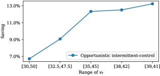
The experimental results are shown in Figure 5. We can observe that when the range of $v_{f}$ becomes smaller, our DRL-based opportunistic intermittent-control approach achieves more fuel consumption savings over only using RMPC. This is because that a smaller range of $v_{f}$ is easier for DRL to learn and leverage.

Figure 5: Fuel consumption savings by our DRL-based opportunistic intermittent-control over RMPC only under different range of $v_{f}$.

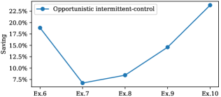
Impact of velocity regularity of Front vehicle. We then conduct experiments to evaluate the impact of the regularity of the Front vehicle velocity, i.e., how “random” the Front vehicle changes its speed. We conduct experiments Ex.6 – Ex.10, which share the same range of $v_{f}$ at $[30,50]$ but with the following differences.

• In Ex.6, $v_{f}$ changes completely random, i.e., a drastic change is allowed instantly;

• Ex.7 shares the same setting with Ex.1, i.e., the velocity can only change continuously;

• In Ex.8, the velocity changes based on Equation (8) but with a large random disturbance. Specifically, the amplitude $a_{f}=5$ and the range of $w$ is $[-5,5]$;

• The setting of Ex.9 is similar to Ex.8, with more regularity, i.e., a larger amplitude $a_{f}=8$ and a smaller disturbance range $[-2,2]$;

• The setting of Ex.10 is similar to Ex.8 and Ex.9, with even more regularity: i.e., $a_{f}=9$ and the disturbance range is $[-1,1]$.

Intuitively, from Ex.6 to Ex.10, the Front vehicle velocity exhibits more regularity. The experiments results are shown in Figure 6. From Ex.7 to Ex.10, we can see that better regularity leads to easier learning of our DRL-based approach and more fuel consumption savings. However, Ex.6 is an exception, where $v_{f}$ is purely random but our approach still achieves significant saving. We speculate that this phenomenon is due to the low performance of the RMPC itself, since there would be a mismatch between the real state and what RMPC predicts.

Figure 6: Fuel consumption savings by our DRL-based opportunistic intermittent-control under different regularity degree of $v_{f}$.

V Conclusion

It is often overly conservative to design safety-critical systems with only the worst-case situations in mind. In this paper, we propose a novel online intermittent-control framework to opportunistically skip the computation and actuation of an underlying safe controller via learning the knowledge of the specific operation context and environment. The framework utilizes both a model-based approach (mixed integer programming formulation) and a learning-based approach (deep reinforcement learning) for different situations to intelligently make the skipping decisions. It also guarantees system safety by formally computing a strengthened safe set based on the notion of robust control invariant and backward reachable set of the underlying controller. Experiments on an adaptive cruise control system demonstrate the effectiveness of our approach in achieving significant energy and computation savings. Future work includes addressing more complex control systems beyond LTI.

References

- [1] L. Chisci, J. A. Rossiter, and G. Zappa, “Systems with persistent disturbances: predictive control with restricted constraints,” Automatica, vol. 37, no. 7, 2001.
- [2] A. G. Richards, “Robust constrained model predictive control,” Ph.D. dissertation, Massachusetts Institute of Technology, 2005.
- [3] J. Löfberg, Minimax approaches to robust model predictive control. Linköping University Electronic Press, 2003, vol. 812.
- [4] M. Hamdaoui and P. Ramanathan, “A dynamic priority assignment technique for streams with (m, k)-firm deadlines,” IEEE Transactions on Computers, vol. 44, no. 12, 1995.
- [5] A. Gujarati, M. Nasri, R. Majumdar, and B. B. Brandenburg, “From iteration to system failure: Characterizing the fitness of periodic weakly-hard systems,” in ECRTS, 2019.
- [6] C. Huang, K. Wardega, W. Li, and Q. Zhu, “Exploring weakly-hard paradigm for networked systems,” in Destion, 2019.
- [7] J. Jiang and X. Yu, “Fault-tolerant control systems: A comparative study between active and passive approaches,” Annual Reviews in Control, vol. 36, no. 1, 2012.
- [8] G. Frehse, A. Hamann, S. Quinton, and M. Woehrle, “Formal analysis of timing effects on closed-loop properties of control software,” in RTSS, 2014.
- [9] P. S. Duggirala and M. Viswanathan, “Analyzing real time linear control systems using software verification,” in RTSS. IEEE, 2015.
- [10] C. Huang, W. Li, and Q. Zhu, “Formal verification of weakly-hard systems,” in HSCC, 2019.
- [11] J. Lan and R. J. Patton, “A new strategy for integration of fault estimation within fault-tolerant control,” Automatica, vol. 69, 2016.
- [12] Y. Song, Y. Wang, and C. Wen, “Adaptive fault-tolerant pi tracking control with guaranteed transient and steady-state performance,” IEEE Transactions on automatic control, vol. 62, no. 1, 2016.
- [13] S. Junges, N. Jansen, C. Dehnert, U. Topcu, and J.-P. Katoen, “Safety-constrained reinforcement learning for mdps,” in TACAS, 2016.
- [14] N. Fulton and A. Platzer, “Safe reinforcement learning via formal methods: Toward safe control through proof and learning,” in AAAI, 2018.
- [15] M. Alshiekh, R. Bloem, R. Ehlers, B. Könighofer, S. Niekum, and U. Topcu, “Safe reinforcement learning via shielding,” in AAAI, 2018.
- [16] D. Krajzewicz, J. Erdmann, M. Behrisch, and L. Bieker, “Recent development and applications of SUMO - Simulation of Urban MObility,” International Journal On Advances in Systems and Measurements, vol. 5, no. 3&4, December 2012.
- [17] M. Rungger and P. Tabuada, “Computing robust controlled invariant sets of linear systems,” IEEE Transactions on Automatic Control, vol. 62, no. 7, 2017.
- [18] E. Asarin, O. Bournez, T. Dang, and O. Maler, “Approximate reachability analysis of piecewise-linear dynamical systems,” in HSCC, 2000.
- [19] S. V. Rakovic, E. C. Kerrigan, K. I. Kouramas, and D. Q. Mayne, “Invariant approximations of the minimal robust positively invariant set,” IEEE Transactions on Automatic Control, vol. 50, no. 3, 2005.
- [20] D. Q. Mayne, J. B. Rawlings, C. V. Rao, and P. O. Scokaert, “Constrained model predictive control: Stability and optimality,” Automatica, vol. 36, no. 6, 2000.
- [21] P. TøNdel, T. A. Johansen, and A. Bemporad, “An algorithm for multi-parametric quadratic programming and explicit mpc solutions,” Automatica, vol. 39, no. 3, 2003.
- [22] C. Huang, X. Chen, Y. Zhang, S. Qin, Y. Zeng, and X. Li, “Hierarchical model predictive control for multi-robot navigation,” in IJCAI, 2016.
- [23] A. Tiwari, “Approximate reachability for linear systems,” in HSCC, 2003.
- [24] H. Van Hasselt, A. Guez, and D. Silver, “Deep reinforcement learning with double q-learning,” in AAAI, 2016.