Minimal matrix product states and generalizations of mean-field and geminal wavefunctions

Abstract

Simple wavefunctions of low computational cost but which can achieve qualitative accuracy across the whole potential energy surface (PES) are of relevance to many areas of electronic structure as well as to applications to dynamics. Here, we explore a class of simple wavefunctions, the minimal matrix product state (MMPS), that generalizes many simple wavefunctions in common use, such as projected mean-field wavefunctions, geminal wavefunctions, and generalized valence bond states. By examining the performance of MMPSs for PESs of some prototypical systems, we find that they yield good qualitative behavior across the whole PES, often significantly improving on the aforementioned ansätze.

I Introduction

Simple qualitative wavefunctions, such as the Slater determinants used in Hartree-Fock (HF) and Kohn-Sham theory, play essential roles in the theory of electronic structure.Ring and Shuck (1980); Blaizot and Ripka (1986); Jensen (2006) For example, they provide qualitative understanding about bonding and structure, and are a starting point for more sophisticated numerical treatments, via perturbation theory or as the dominant component in a more flexible ansatz. In addition, because computations with such wavefunctions are cheap (often $N^{3}$ or $N^{4}$ cost where $N$ is proportional to system size) such wavefunctions may be used both to study large systems, and to study dynamics, where cheap electronic structure methods are essential.

Beyond Slater determinants, other simple wavefunctions in common use can be thought of as small generalizations. One class is obtained by breaking and restoring the symmetries in a Slater determinant.Li and Chan ; Ring and Shuck (1980); Blaizot and Ripka (1986); Scuseria et al. (2011); Thompson and Hratchian (2019); Qiu, Henderson, and Scuseria (2016); Lykos and Pratt (1963); Mayer (1980); Löwdin (1955) For example, typical Hamiltonians conserve particle number ($N$), spin symmetry ($S^{2}$, $S_{z}$), and time reversal symmetry, in addition to various point group symmetries. Rather than using a Slater determinant that obeys all these symmetries, one can break the symmetries in order to capture essential correlations, and then restore them using projectors. This leads to a variety of wavefunctions, such as projected unrestricted Hartree-Fock Löwdin (1955); Lykos and Pratt (1963); Mayer (1980) (broken and restored spin symmetry), the antisymmetrized geminal power (AGP) (broken and restored number symmetry),Coleman (1965); Mang (1975); Ring and Shuck (1980); Blaizot and Ripka (1986) and, as an extension to AGP, projected Hartree-Fock-Bogoliubov (HFB).Ring and Shuck (1980); Sheikh and Ring (2000); Scuseria et al. (2011) These wavefunctions are easy to compute with, because their mean-field origin means that matrix elements can be obtained by a modified Wick’s theorem. Another way to create a simple wavefunction is to construct a product state not of orbitals, but of multi-electron objects. The generalized valence bond (GVB) state is one such example, corresponding to a product state of strongly orthogonal two-particle (geminal) wavefunctions.Hurley, Lennard-Jones, and Pople (1953); Goddard (1967); Goddard and Ladner (1971); Goddard et al. (1973); Wu et al. (2011); Rassolov (2002); Jensen (2006); Cullen (1996); Johnson et al. (2017); Limacher (2016)

In this work, we describe another convenient way to generate simple wavefunctions using the formalism of matrix product states (MPSs), the wavefunction ansatz of the density matrix renormalization group (DMRG).Schollwöck (2011); White (1992, 1993); Chan and Sharma (2011); Baiardi and Reiher (2020); Szalay et al. (2015) Matrix product states provide several ways to generalize the above pictures. First, they allow for expectation values to be efficiently evaluated without the structure of a generalized Wick’s theorem. Second, it is natural to work with products of many-particle objects in the MPS form. Third, by increasing the MPS bond dimension $D$ (defined below) one can easily incorporate correlations beyond those purely from symmetry projection, or contained within the individual wavefunction components (be they orbitals, geminals, or more complex objects). Given the second quantized Hamiltonian, the cost of a MPS calculation scales like $K^{4}$ (where $K$ is the number of orbitals) with a prefactor that depends polynomially on the dimension $D$ of the matrices that are the variational parameters of the state.White and Martin (1999); Chan and Head-Gordon (2002); Chan (2004); Szalay et al. (2015) While in typical DMRG calculations, the bond dimension is made very large in order to provide near exact answers, in the current work we focus on the opposite limit where $D$ is very small, e.g. $\mathcal{O}(1)$, and thus the prefactor in front of $K^{4}$ is very small. We shall call such states minimal matrix product states (MMPS). As we shall see, in conjunction with symmetry projection, even the smallest minimal matrix product state with $D=1$ already encompasses the simple wavefunctions in common use, while generalizing to new classes of simple wavefunctions that have not previously been considered.

The remainder of this article is organized as follows: Section II gives an overview of the MMPS ansatz in (Section II.1), its connection to geminal and related ansätze (Section II.2), and describes the algorithmic implementation of the MMPS ansatz (Section II.3). Section III presents MMPS results for some prototypical systems and compares them to results from related ansätze. Section IV concludes and gives our outlook on future applications.

II Theory

II.1 Minimal matrix product state ansatz

A matrix product state is obtained by writing the amplitude of a wavefunction as a product of matrices $\mathbf{A}^{n_{i}}$, namely, for $K$ orbitals

$$|{\Psi_{\mathrm{MPS}}}\rangle=\sum_{\{n\}}\mathbf{A}^{n_{1}}\mathbf{A}^{n_{2}}\ldots\mathbf{A}^{n_{K}}|{n_{1}n_{2}\ldots n_{K}}\rangle$$ ((1))

where $|{n_{1}n_{2}\ldots n_{K}}\rangle$ is an occupancy vector for sites $1\ldots K$.Chan and Sharma (2011); Schollwöck (2011); Szalay et al. (2015) In the simplest case we consider, we assume that the basis of site $i$ is a single orbital, i.e. $\{|{n_{i}}\rangle\}=\{|{\mathrm{vac}}\rangle,|{\phi_{i}^{\alpha}}\rangle,|{\phi_{i}^{\beta}}\rangle,|{\phi_{i}^{\alpha}\phi_{i}^{\beta}}\rangle\}$. In a restricted formalism (used here) we further assume $\langle r\alpha|\,\phi_{i}^{\alpha}\rangle=\langle r\beta|\,\phi_{i}^{\beta}\rangle$. The representational power of the MPS is controlled by the bond dimension of the matrices, which is $D\times D$ save for the first and last which are $1\times D$ and $D\times 1$.

The smallest matrix product state is the simple product state with $D=1$, i.e. $\mathbf{A}^{n_{i}}$ is a scalar for each element of the site basis. Such a state will not generally respect the symmetries of the system. Consequently, we define a minimal matrix product state as the state obtained from the product state after an additional projection onto the pure symmetry sectors of the Hamiltonian. In this work, we consider Hamiltonians where $N$, $S^{2}$ and $S_{z}$ are good quantum numbers. Thus we define the minimal matrix product state to conserve one or more of these symmetries, e.g.

$$|\Psi_{\text{MMPS}}\rangle=\hat{P}|{\Psi_{\text{MPS}}}\rangle=\hat{P}^{S^{2},S_{z}}\hat{P}^{N}|\Psi_{\text{MPS}}\rangle$$ ((2))

where e.g. $\hat{P}^{N}$ denotes projection onto a given particle number $N$. Note that the distinction between MMPS and earlier projected matrix product states such as the spin-projected MPS Li and Chan ; Li et al. (2019) is mainly one of emphasis on using the smallest bond dimensions. While $|\Psi_{\text{MMPS}}\rangle$ is itself an MPS of a bond dimension given by that of the $|\Psi_{\text{MPS}}\rangle$ multiplied by that of the projector $\hat{P}$, the explicit larger representation never needs to be formed in standard computations (see Section II.3 for more details).

It is useful to contrast the above scheme with how symmetries are usually expressed in MPSs without projection.Schollwöck (2011); Chan and Head-Gordon (2002); Sharma and Chan (2012); Keller and Reiher (2016); Szalay et al. (2015) For Abelian symmetries, such as $N$ and $S_{z}$, so long as $\{|n_{i}\rangle\}$ are eigenstates of $\hat{N}$ and $\hat{S}_{z}$, one can ensure that $|\Psi_{\mathrm{MPS}}\rangle$ is an irrep of these symmetries by requiring that the matrices $\mathbf{A}^{n_{i}}$ have a block structure. Choosing reasonable sizes for such quantum number blocks is a discrete optimization process that is challenging when the total bond dimension is small. In the projection approach, the need to choose a block structure is avoided, which thus allows meaningful calculations with very small bond dimension, as small as $D=1$.

From the above definition of a MMPS, we can extend the ansatz in two natural ways. The first way is to enlarge the definition of a site in the underlying MPS to capture the Hilbert space of multiple spin orbitals. For example, we may consider grouping pairs of the above sites into single sites, e.g. $\{|n_{i}n_{i+1}\rangle{\}}\to{\{}|\tilde{n}_{i/2}\rangle{\}}$, where the dimension of $\{{|{\tilde{n}_{i/2}}\rangle}\}$ is now 16. The parent MPS is then still a product state, but of more complex components, similar to e.g. a GVB state. We shall refer to such MMPS as multisite MMPS. The second way is to increase the bond dimension of $\mathbf{A}^{n_{i}}$ (i.e. they become matrices) in the typical way that matrix product states are made more accurate. As explained in the introduction, in this work we will focus on the case of small bond dimensions e.g. $D=1-5$, keeping the ansatz as minimal as possible. In the evaluation of the computational costs (see Section II.3), $D$ thus enters only as a small prefactor.

It is important to note that, similar to normal MPS with insufficiently large $D$, the MMPS is not invariant to orbital transformations between sites (including the ordering of the sites). Thus, as is the case for other simple wavefunctions, its quality depends heavily on the orbitals used to define it. In numerical calculations, orbital optimization is thus often a necessary consideration.

II.2 Exponential form and connection to geminal powers and other ansätze

To more easily connect the $D=1$ MMPS to other commonly used simple wavefunctions, we first write it in another explicit form. For the most direct correspondence, we first consider the case where the sites are single orbitals. Then,

$$|\Psi_{\text{MMPS}}\rangle=\hat{P}\mathcal{T}\prod_{i}(c_{i}+s_{i\alpha}\hat{a}^{\dagger}_{i\alpha}+s_{i\beta}\hat{a}^{\dagger}_{i\beta}+d_{i}\hat{a}^{\dagger}_{i\alpha}\hat{a}^{\dagger}_{i\beta})|\mathrm{vac}\rangle$$ ((3))

where the ordering operator $\mathcal{T}$ ensures that the non-commuting single creation operators are applied in lexicographical order (note that the constants and double creation operators commute with each other and all single creation terms) e.g.

$$\mathcal{{T}}\prod_{i\sigma}\hat{a}^{\dagger}_{i\sigma}=\hat{a}^{\dagger}_{1\alpha}\hat{a}^{\dagger}_{1\beta}\hat{a}^{\dagger}_{2\alpha}\hat{a}^{\dagger}_{2\beta}\ldots$$ ((4))

For the sites where $c_{i}\neq 0$, we can rewrite the factors in Eq.  (3) as exponentials since $ce^{c^{-1}({s}_{\alpha}\hat{a}^{\dagger}_{\alpha}+{s}_{\beta}\hat{a}^{\dagger}_{\beta}+{d}\hat{a}^{\dagger}_{\alpha}\hat{a}^{\dagger}_{\beta})}=c+s_{\alpha}\hat{a}^{\dagger}_{\alpha}+s_{\beta}\hat{a}^{\dagger}_{\beta}+d\hat{a}^{\dagger}_{\alpha}\hat{a}^{\dagger}_{\beta}$. Thus if all $c_{i}\neq 0$, the $D=1$ MMPS is an ordered exponential up to a scaling factor,

$$|\Psi_{\text{MMPS}}\rangle=\hat{P}\mathcal{T}e^{\sum_{i\sigma}s_{i\sigma}\hat{a}^{\dagger}_{i\sigma}+\sum_{i}d_{i}\hat{a}^{\dagger}_{i\alpha}\hat{a}^{\dagger}_{i\beta}}|\mathrm{vac}\rangle$$ ((5))

The general AGP ansatz in its canonical basis (i. e., after an appropriate orbital rotation) with $N_{s}$ singly occupied orbitals can be written as

$$|{\Psi_{\text{AGP}}}\rangle=\hat{P}^{N}\mathcal{T}\prod_{i=1}^{N_{s}}\hat{a}^{\dagger}_{i\alpha}\prod_{i={N_{s}+1}}^{K}\left(1+d_{i}\hat{a}^{\dagger}_{i\alpha}\hat{a}^{\dagger}_{i\beta}\right)|{\text{vac}}\rangle$$ ((6))

Comparing this to the MMPS form of Eq.  (3) we see the MMPS reduces to the general AGP if for $N_{s}$ of the factors, we only have one coefficient $s_{i\sigma}$ per factor, while for the other factors, we only have the constant $c_{i}$ and double creation $d_{i}$ term, reproducing the geminal terms in Eq.  (6). Consequently, we refer to the latter factors as the geminal part of the MMPS wavefunction.

Since the single site $D=1$ MMPS is distinguished from the AGP by the way in which the single creation operators enter into the ansatz, we can compare also to some other wavefunctions which are related to the AGP but which introduce single creation operators in a different way. Fukutome and coworkers introduced a generalization of the Bardeen-Cooper-Schrieffer wavefunction (the AGP before projection) with single creation operators in an exponential,Fukutome, Yamamura, and Nishiyama (1977); Fukutome (1981) written as

$$|\Psi_{\text{F}}\rangle=e^{\sum_{i}(\theta_{i}\hat{a}^{\dagger}_{i}-\theta_{i}^{*}\hat{a}_{i})}e^{\sum_{i}d_{i}\hat{a}^{\dagger}_{i\alpha}\hat{a}_{i\beta}}|\mathrm{vac}\rangle$$ ((7))

where $\theta_{i}$ are complex numbers. However, note that $e^{\sum_{i}(\theta_{i}\hat{a}^{\dagger}_{i}-\theta_{i}^{*}\hat{a}_{i})}=c_{0}+\sum_{i}(c_{i}\hat{a}^{\dagger}_{i}-c_{i}^{*}\hat{a}_{i})$ for some constants $c_{0},c_{i}$, thus this is very different from the MMPS where there is an ordered exponential; in particular, unlike in the MMPS, if $d_{i}=0$ it is not possible for the single creation operators to create a state with more than a single particle. Finally we note that exponentials of single creation operators also occur in fermion coherent states similarly to in Eq.  (7), but there $\theta_{i},\theta_{i}^{*}$ are Grassman numbers.Blaizot and Ripka (1986) This ensures that expectation values with fermion coherent states satisfy Wick’s theorem for expectation values (i.e. expectation values of fermionic operators can be expressed in terms of sums of products of single-particle density matrices) but it also means that the amplitude of a fermionic coherent state is not physically meaningful, as it is a Grassman number.

To understand the variational freedom introduced by the single creation operators in the MMPS, we can consider a simple limiting case where the geminal coefficients $d_{i}$ are 0 in Eq.  (5). This corresponds to assuming all wavefunction amplitudes can be factorized as

$$\left\langle\phi_{i_{1}}^{\sigma_{i_{1}}}\phi_{i_{2}}^{\sigma_{i_{2}}}\ldots\phi_{i_{N}}^{\sigma_{i_{N}}}\vphantom{\phi_{i_{1}}^{\sigma_{i_{1}}}\phi_{i_{2}}^{\sigma_{i_{2}}}\ldots\phi_{i_{N}}^{\sigma_{i_{N}}}\Psi}\left|\,\Psi\vphantom{\phi_{i_{1}}^{\sigma_{i_{1}}}\phi_{i_{2}}^{\sigma_{i_{2}}}\ldots\phi_{i_{N}}^{\sigma_{i_{N}}}\Psi}\right.\right\rangle=s_{i_{1}\sigma_{i_{1}}}s_{i_{2}\sigma_{i_{2}}}\dots s_{i_{N}\sigma_{i_{N}}}$$ ((8))

The representational power of such a form is highly limited; it is not possible to doubly occupy any spatial orbital. There are nonetheless some non-trivial states that can be captured in this way. In general, if we assume each $\alpha$ and $\beta$ orbital has the same spatial component, then the single creation operators create an orbital of rotated spin (a generalized spin orbital),

$$\sum_{\sigma}s_{i\sigma}\hat{a}^{\dagger}_{i\sigma}|\mathrm{vac}\rangle=\sqrt{\sum_{\sigma}|s_{i\sigma}|^{2}}|{\phi}_{i}^{\bar{\sigma}_{i}}\rangle$$ ((9))

where $\bar{\sigma}$ denotes the rotated spin. Incorporating projection onto fixed $N$, then the MMPS becomes a weighted distribution over $N$-particle products of generalized spin orbitals

$$\begin{split}|{\Psi}\rangle=\sum_{i_{1}=1}^{K}&\sum_{\begin{subarray}{c}i_{2}=2\\ i_{2}\neq i_{1}\end{subarray}}^{K}\sum_{\begin{subarray}{c}i_{3}=3\\ i_{3}\notin\{i_{1},i_{2}\}\end{subarray}}^{K}\cdots\sum_{\begin{subarray}{c}i_{N}=N\\ i_{N}\notin\{i_{1},i_{2},\cdots,i_{N-1}\}\end{subarray}}^{K}\\ &c_{i_{1}}c_{i_{2}}\cdots c_{i_{N}}|{\phi_{i_{1}}^{\bar{\sigma}_{i_{1}}}\phi_{i_{2}}^{\bar{\sigma}_{i_{2}}}\ldots\phi_{i_{N}}^{\bar{\sigma}_{i_{N}}}}\rangle\end{split}$$ ((10))

where $c_{i}=\sqrt{\sum_{\sigma}|s_{i\sigma}|^{2}}$. For any $K>N$, this represents a non-trivial linear combination; for example, for $K=3$ and $N=2$, we get $|{\Psi}\rangle=c_{1}c_{2}|{\phi_{1}^{\bar{\sigma}_{1}}\phi_{2}^{\bar{\sigma}_{2}}}\rangle+c_{1}c_{3}|{\phi_{1}^{\bar{\sigma}_{1}}\phi_{3}^{\bar{\sigma}_{3}}}\rangle+c_{2}c_{3}|{\phi_{2}^{\bar{\sigma}_{2}}\phi_{3}^{\bar{\sigma}_{3}}}\rangle$. Thus even this artifically simple ($d_{i}=0$) example of an MMPS describes physics different than that of other mean-field and projected mean-field states.

As another example, note that an AGP state is written as a linear combination of all doubly occupied determinants but the AGP ansatz does not include determinants from higher seniority sectors. In the MMPS, the inclusion of the single creation operators via the ordering operator $\mathcal{T}$ yields a state that can formally access all determinants in the Hilbert space.

Multisite MMPS, as well as bond dimensions with $D>1$ have the potential to compactly represent even more qualitative electronic structures beyond that captured by the AGP language. For example, the perfect pairing GVB wavefunction Jensen (2006); Wu et al. (2011) can be written (up to normalization) as

$$|\Psi_{\mathrm{GVB}}\rangle=\prod_{i=1}^{K/2}(\hat{a}^{\dagger}_{i\alpha}\hat{a}^{\dagger}_{i\beta}+d_{i}\hat{a}^{\dagger}_{\bar{i}\alpha}\hat{a}^{\dagger}_{\bar{i}\beta})|\mathrm{vac}\rangle$$ ((11))

where indices $i,\bar{i}$ index the perfect pairing orbitals. As this is a product state, it is clearly a matrix product state, and if the MPS sites are chosen to consist of the paired orbitals $\{\phi_{i\sigma},\phi_{\bar{i}\sigma^{\prime}}\}$ then it is a MPS (and thus MMPS) of bond dimension 1. However, it is easy to generalize the perfect pairing GVB wavefunction now also to include broken pairs by including the linear terms in the MMPS ansatz, or to include broken and restored symmetries, or to include clusters of larger sites. The key point is that formulating the ansatz in the matrix product language provides a simple organization of the computation, which does not require the unprojected state to obey Wick’s theorem for expectation values (as for projected mean-field and AGP states) or to be a single product state (as for GVB).

As with many of the other wavefunction ansätze discussed, MMPS (and MPS) are not size consistent in general. For normal MPS, size consistency requires an appropriate choice of orbitals and their ordering. For the MMPS, size consistency is broken by the projector but recovered (for the appropriate choice of orbitals and ordering) in the large $D$ limit. Nonetheless, in many cases of interest the extensive scaling of the correlation energy is less important than the treatment of the intensive changes in the correlation energy in a local region where bonds are changing, which the MMPS can recover using orbitals localized to that region. In addition, by imposing local particle number constraints on the projector, global size consistency can be restored, as has been demonstrated with the Jastrow-AGP ansatz.Neuscamman (2012) However, this is beyond the scope of this work.

II.3 Implementation

The variationally minimized energy of the MMPS ansatz Eq.  (2) can be carried out using the following functional Ring and Shuck (1980)

$$E=\text{min}_{\Psi_{\text{MPS}}}\frac{\langle{\Psi_{\text{MPS}}}|{\hat{H}\hat{P}}|{\Psi_{\text{MPS}}}\rangle}{\langle{\Psi_{\text{MPS}}}|{\hat{P}}|{\Psi_{\text{MPS}}}\rangle},$$ ((12))

where we have used the fact that $\hat{P}$ commutes with $\hat{H}$ and idempotency of $\hat{P}$. Note that $|{\Psi_{\text{MMPS}}}\rangle$ does not explicitly appear in Eq.  (12) and thus does not need to be constructed. In the following, we describe possible numerical choices of $\hat{P}$ and the implementation of Eq.  (12).

II.3.1 Choice of projector

There are many ways to evaluate the expectation value of a projected wavefunction occurring in Eq.  (12). For example, in variational Monte Carlo, one samples the wavefunction using states that have the desired symmetries.Casula and Sorella (2003); Casula, Attaccalite, and Sorella (2004); Sandvik and Vidal (2007); Neuscamman, Umrigar, and Chan (2012); Mahajan and Sharma (2019); Dobrautz, Smart, and Alavi (2019) Here, we use an explicit operator representation of the projector. Formally, a projector is a delta distribution that selects the eigenstates to project on.Ring and Shuck (1980); Izmaylov (2019) For example, $\hat{P}^{N}=\delta(\hat{N}-N)$ where $\hat{N}=\sum_{i}\hat{n}_{i}=\sum_{i}\hat{a}^{\dagger}_{i}\hat{a}_{i}$. We consider two explicit constructions of the projector: a matrix-product-operator Schollwöck (2011) (MPO) construction, and an integral-based construction.

To illustrate the idea behind the MPO construction, we consider the representation of $\hat{P}^{N}$. We define our MPO projector such that applying $\hat{P}^{N}$ to the MPS formally yields an MMPS with the same structure as ordinary MPS with quantum numbers, i.e. the matrices $A^{n_{i}}$ have a block-structure labelled by particle number. A pictorial example is shown in Fig.  1.

To obtain the projector, we first, as in conventional DMRG,Hu and Chan (2015); Szalay et al. (2015) construct all possible particle sectors for a given bond such that the initial site starts with $0$ and the last site ends with $N$ electrons (compare with Fig.  1 for $N=2$). The number of particle sectors on the bond corresponds then to the dimension of the MPO on that bond. The MPO tensor on a site $i$ is a matrix for each bra, ket pair $n_{i},n_{i}^{\prime}$ in the basis of site $i$, and to satisfy particle number balance the elements of the tensor take the form

$$[\mathbf{M}^{n_{i},n_{i}^{\prime}}]_{lr}=\delta_{n_{i}n_{i}^{\prime}}\delta_{N(l)+N(n_{i}),N(r)},$$ ((13))

where $N(n_{i})$ is the number of particles in state $|n_{i}\rangle$ i.e, $\{0,1\}$ for one spin orbital, and $N(l)$ and $N(r)$ are the number of particles associated with the left bond index $l$ and right bond index $r$ of the MPO tensor.

For $\hat{P}^{N}$, the maximal bond dimension (maximal number of particle sectors at a given bond) is $D_{P}^{(N)}=N+1$ (this is the total number of partitions of $N$ between the left and right halves of the system, i.e. $(0,N),(1,N-1),\ldots(N,0)$). Generalizing to a projector that fixes both $S_{z}$ and $N$, $\hat{P}^{N_{\alpha}}\hat{P}^{N_{\beta}}=\hat{P}^{S_{z}}\hat{P}^{N}$, the maximal bond dimension becomes $D_{P}^{(N_{\alpha},N_{\beta})}=$$(N_{\alpha}+1)(N_{\beta}+1)$. The projector can be generalized to $S^{2}$ symmetry by defining the tensor elements in Eq.  (13) in terms of the Wigner $3j$ symbols. The MPO projector form has the property that the symmetry is directly encoded in the block structure of the MPO. However, while it works well in its exact form, we have found that it is not so easy to approximate at lower cost, as “pruning” the projector does not preserve the commutation betwen $\hat{H}$ and $\hat{P}$, required for the variational bound on the energy functional in Eq.  (12).

Figure 1: Diagram of the matrix-product-operator (MPO) based projector $P$ for constraining particle-number symmetry in the minimal matrix product state (MMPS). Applying $\hat{P}$ to the MPS (right-hand side) generates a MMPS (left-hand side). The MMPS formally corresponds to a MPS whose matrices are in block-sparse form with equally sized blocks, where each block is labelled by the combinations of particle numbers along the arrows. The arrows denote the “flow” of particles. The sets denote the particle number sectors on a particular bond in the MPS. An example is shown for $N=2$ and four spin orbitals/sites.

Alternatively, the projector can be constructed in an integral representation.Ring and Shuck (1980); Mang (1975) For $\hat{P}^{N}$, this takes the form

$$\hat{P}^{N} =\frac{1}{2\pi}\int_{0}^{2\pi}\exp[\mathrm{i}\phi(\hat{N}-N)]\mathrm{d}\phi.$$ ((14))

Discretizing the integral with $N_{\text{grd}}$ grid points gives

$$\hat{P}^{N} =\frac{1}{N_{\text{grd}}}\sum_{n=0}^{N_{\text{grd}}-1}\exp[\mathrm{i}\phi_{n}(\hat{N}-N)]=\delta_{\hat{N},N},$$ ((15))

with $\phi_{n}=2\pi n/{N_{\text{grd}}}$. Since $\exp(\mathrm{i}\phi\hat{N})=\exp(\mathrm{i}\phi\sum_{i}\hat{n}_{i})=\prod_{i}\exp(\mathrm{i}\phi\hat{n}_{i})$, $\hat{P}^{N}$ can be written as sum of products i.e., a sum of MPOs with $D=1$, or a single sparse MPO with bond dimension $N_{\text{grd}}$.Li and Chan This allows for an embarrassingly parallel implementation. While the overall $\hat{P}^{N}$ is real-valued, the individual terms $\exp(\mathrm{i}\phi\hat{N})$ in Eq.  (15) are complex-valued. However, to avoid complex algebra, Eq.  (15) can be recast into a sum over $N_{\text{grd}}/2$, $D=2$ real-valued MPOs, plus one $D=1$ MPO term (or a single block-sparse MPO with bond dimension $N_{\text{grd}}+1$) by using only the real-valued part of the individual terms:

$$\hat{P}^{N} =\frac{1}{N_{\text{grd}}}\sum_{n=0}^{N_{\text{grd}}-1}\cos[\phi_{n}(\hat{N}-N)]$$ ((16))

$$=\frac{1}{N_{\text{grd}}}\hat{1}+\frac{2}{N_{\text{grd}}}\sum_{n=1}^{N_{\text{grd}}/2}\cos[\phi_{n}(\hat{N}-N)]$$ ((17))

where we made use of the periodicity and the even symmetry of the $\cos$ function and assumed odd $N_{\text{grd}}$. $\cos[\phi_{n}(\hat{N}-N)]$ can then be written as an MPO via

$$\begin{bmatrix}c(\hat{n}_{1}^{\prime}\phi_{n})&s(\hat{n}_{1}^{\prime}\phi_{n})\end{bmatrix}\begin{bmatrix}c(\hat{n}_{2}^{\prime}\phi_{n})&s(\hat{n}_{2}^{\prime}\phi_{n})\\ -s(\hat{n}_{2}^{\prime}\phi_{n})&c(\hat{n}_{2}^{\prime}\phi_{n})\end{bmatrix}\cdots\begin{bmatrix}c(\hat{n}_{K}^{\prime}\phi_{n})\\ -s(\hat{n}_{K}^{\prime}\phi_{n})\end{bmatrix}$$ ((18))

where we have used the shorthand $c(\phi)=\cos\phi$, $s(\phi)=\sin(\phi)$ and $\hat{n}_{i}^{\prime}=\hat{n}_{i}-N/K$.

While we found numerically, for the cases we have studied (up to $K=8$ and $N=8$), that the complex-valued sum can also be fitted into a real-valued sum (of $D=1$ MPOs) with twice as many terms, the numerical fitting procedure Kolda and Bader (2009) is difficult and not well-conditioned if $K$ is large. Thus, we leave the question of other simple, analytical real-valued descriptions of Eq.  (15) for future considerations. Instead, in the following we stick to the slightly more computationally demanding real-valued $D=2$-MPO-form, which has off-diagonal terms in each MPO.

Similarly to $\hat{P}^{N}$, a projector onto fixed $S_{z}$ and $S^{2}$ can also be constructed in integral form Ring and Shuck (1980); Li and Chan ; Scuseria et al. (2011)

$$\hat{P}^{S^{2},S_{z}} =\hat{P}^{S_{z}}\hat{\mathcal{P}}^{S^{2}}\hat{P}^{S_{z}},$$ ((19))

$$\hat{\mathcal{P}}^{S^{2}} =\frac{2S+1}{2}\int_{0}^{\pi}\sin(\alpha)d_{M,M}^{S}(\alpha)\exp(-\mathrm{i}\alpha\hat{S}_{y})\mathrm{d}\alpha,$$ ((20))

where $d_{M,M}^{S}$ is the small Wigner-D matrix.Joachain (1975) $\hat{\mathcal{P}}^{S^{2}}$ is not a true projector and mixes spin orbitals, thus $\hat{P}^{S_{z}}$ has to be applied twice in Eq.  (19) in order to ensure that $\hat{P}^{S^{2},S_{z}}$ is a projector. $\hat{P}^{S_{z}}$ is defined analogously to $\hat{P}^{N}$ and can be implemented in the same manner. $\hat{P}^{S^{2}}$ can be evaluated via Gauß-Legendre quadrature and results in a real-valued sum of terms. The number of quadrature points required to evaluate the integral exactly is stated in Ref. [​​4] and is proportional to the number of singly occupied orbitals and the $S$ value.

One advantage of the integral based construction is that one can easily obtain approximate projectors of lower cost by reducing the number of grid points $N_{\text{grd}}$ in the integration. Although the approximate projectors no longer commute with $\hat{H}$ exactly, we have found this to be less of an issue in practice than for the MPO based projector. We note that sufficient grid points have to be chosen for $\hat{P}^{S_{z}}$ in order to achieve idempotency of $\hat{P}^{S^{2},S_{z}}$. In contrast, regardless of the number of grid points, $\hat{P}^{S_{z}}$ and $\hat{P}^{N}$ are always idempotent as they project onto $S_{z}$ or $N$ modulo $N_{\text{grd}}$.

II.3.2 DMRG algorithm

The standard way to optimize the energy of an MPS ansatz is the DMRG algorithm, where, similar to an alternating least squares algorithm,Kolda and Bader (2009) one optimizes a small number of (neighboring) sites $\{\mathbf{A}^{n_{i}},\mathbf{A}^{n_{i+1}},\dots,\mathbf{A}^{n_{i+x}}\}$ at a time while fixing the remaining sites $\{\mathbf{A}^{n_{1}},\dots,\mathbf{A}^{n_{i-1}},\mathbf{A}^{n_{i+x+1}},\dots,\mathbf{A}^{n_{K}}\}$.White (1992, 1993) This local optimization problem is quadratic and can be solved as an eigenvalue problem. After some sites are optimized, the next neighboring sites are chosen until all sites in the MPS have been optimized. This is called a sweep and repeated until convergence.

For quantum-chemical Hamiltonians, the DMRG algorithm can be efficiently implemented using complementary operators.Xiang (1996); White and Martin (1999); Chan (2004) The complementary operators consist of a precontraction of some of the terms in the Hamiltonian which provide an optimal way to use the sparsity existing in the Hamiltonian’s MPO representation.Keller et al. (2015); Chan et al. (2016) Here, to optimize the energy functional in Eq.  (12) for the MMPS, we implemented a new DMRG code. Specifically, we use a generalized implementation that evaluates Eq.  (12) using the combined operator $\hat{H}\times\hat{P}$ within the complementary operator approach. $\hat{P}$ is constructed using either the MPO or integral based construction as described in Section II.3.1 and is a sparse MPO of bond dimension $D_{P}$. Because of the sparsity of the representation of $\hat{P}$, the MPO tensors have only $\mathcal{O}(D_{P})$ non-zero entries.

Compared to a conventional DMRG implementation without $\hat{P}$, for each complementary operator of the Hamiltonian on a given site, there are $D_{P}$ associated terms to be stored. (The number of terms is proportional to $D_{P}$ rather than $D_{P}^{2}$ due to the MPO sparsity). Further, the individual terms in $[\mathbf{PH}]$ are non-symmetric as, e.g. $\hat{a}^{\dagger}_{i}\hat{P}\neq\hat{P}\hat{a}^{\dagger}_{i}$. Hence, compared to a normal DMRG implementation, $2D_{P}$ more terms need to be computed. Note, however, that the formal bond dimension of the MMPS, obtained by applying $\hat{P}$ to the underlying MPS of bond dimension $D$, is $D\times D_{P}$, and the cost of optimizing the MMPS is much cheaper than the cost of a DMRG computation with a general MPS of bond dimension $D\times D_{P}$. The reduced cost can be understood in terms of the smaller number of parameters to be optimized (smaller matrices to be diagonalized) and by the simple form of $\hat{P}$. Whereas in conventional DMRG, all $D_{P}$ blocks of size $D\times D$ contain different values in the block-sparse MPS, in the MMPS, the blocks are all generated via $\hat{P}$ from a single block. Essentially, introducing $\hat{P}$ shifts some computational effort from the MPS to the operator, at the cost of some restriction in the degrees of freedom.

To allow for multisite MMPSs, we generalized the code to include an arbitrary selection of determinants on a given site. For $D=1$ this also enables AGP, GVB and similar wavefunction optimization, while for $D>1$ one can optimize in the subspace of determinants included in the AGP or GVB ansätze.

With the aforementioned modifications, the remainder of the optimization can follow the normal DMRG algorithm. Here, we used the one-site algorithm, where just one site is optimized at a time, in combination with perturbative noise to avoid getting stuck in local minima.White (2005) For optimizing a particular site $i$, a generalized eigenvalue problem results from Eq.  (12):

$$[\mathbf{HP}]\mathbf{A}^{n_{i}}=\mathbf{P}\mathbf{A^{n_{i}}}E.$$ ((21))

Due to the null space of $\hat{P}$, the matrices $[\mathbf{HP}]$ and $\mathbf{P}$ are indefinite and share the same null space. For some methods, this null space needs to be projected out.Tsuchimochi and Ten-no (2019) Here, this costly projection can be avoided by using the Davidson method Davidson (1975) for generalized eigenvalue problems and by using an initial trial solution $\tilde{\mathbf{A}}^{n_{s}}$ that is an element of the kernel of $\hat{P}$. Only for poor approximations of $\hat{P}$ with insufficient quadrature points did we find numerical issues due to the null space of $\hat{P}$.

In most situations, even for a $D=1$ MMPS with only four parameters per site, the one-site DMRG algorithm performed well as an optimization algorithm in our studies. However, especially when non-optimal orbitals were used for the MMPS, a gradient-based optimization of the MMPS parameters instead of a DMRG optimization turned out to be more efficient in some cases. In practice, for these difficult cases, we used a combination of both DMRG and gradient-based trust-region methods.Nocedal and Wright (2006) For difficult cases such as the H4 system with AGP orbitals, we also performed basin hopping to avoid getting stuck in high-lying local minima.Wales and Doye (1997)

Orbital optimization was performed using the PySCF quantum chemistry package,Sun et al. ; Sun et al. (2020) which requires the one- and two-body density matrices as input.Sun, Yang, and Chan (2017) These we computed as expectation values of the MMPS wavefunction.

II.3.3 Computational cost

Following the scaling analysis of the standard quantum-chemistry DMRG algorithm,Chan and Head-Gordon (2002); Chan (2004); Szalay et al. (2015) the computational cost of evaluating and optimizing the MMPS energy in Eq.  (12) (given the second quantized integrals) scales as $\mathcal{O}[C(K^{3}D^{3}+K^{4}D^{2})]$, where $C$ is the cost of applying the projector. Here, the bond dimension $D$ is of $\mathcal{O}(1)$ so we write the cost more succinctly as $\mathcal{O}(CK^{4})$. This scaling is the same as that of projected HFB, AGP, and other related methods. If orbital optimization is performed, there is an additional $K^{5}$ cost from the integral transformation in each orbital optimization step.

Because the projector is sparse in both the MPO and integral construction, $C$ is directly proportional to the projector bond dimension $D_{P}$. Thus for exact projectors, $C$ depends on the number of symmetries projected against. For example, if we use $\hat{P}=\hat{P}^{S_{z}}\hat{P}^{N}$, then for the MPO construction $C\propto N_{\alpha}N_{\beta}$, while for the integral form $C\propto N_{\text{grd}}=K^{2}$. As mentioned above, we observe that approximate projectors constructed in the integral form by using a reduced number of grid points $N_{\text{grd}}$ in practice work quite well. Indeed, for mean-field-like methods such as HFB it has been observed that the required $N_{\text{grd}}$ scales better than linearly with system size for $\hat{P}^{N}$.Scuseria et al. (2011) Also sparse cubature can reduce $N_{\text{grd}}$ for spin projection in HF.Lestrange et al. (2018) However, we are not aware of rigorous studies of the scaling of the approximation error with system size due to a reduced $N_{\text{grd}}$, and we leave this question for future considerations.

III Results

We now study the behavior of the MMPS and the multisite MMPS (i.e. where a single site spans multiple orbitals) for some prototypical problems that exhibit static correlation, and compare to results from similar ansätze such as GVB and AGP. The systems we study are the H4 ring (Section III.1), O2 dissociation (Section III.2), and HF dissociation (Section III.3).

If not mentioned otherwise, the projector used for the MMPS is $\hat{P}=\hat{P}^{S_{z}}\hat{P}^{N}$. For this projector, we use the MPO form defined in Section II.3.1. We will also use $\hat{P}=\hat{P}^{S^{2},S_{z}}\hat{P}^{N}$. In this case, we employ the integral form defined in Section II.3.1 with $N_{\text{grd}}=5$ grid points for the $N$ and $S_{z}$ integrations, and $N_{\text{grd}}=2$ grid points for the $S^{2}$ integration. Unless stated otherwise, orbitals in the MMPS calculations were ordered according to canonical order (energy order for HF orbitals, natural orbital occupancy for AGP orbitals, and in the same order as the starting orbitals when using optimized orbitals).

Both MMPS and GVB optimization used the code described in Section II.3. AGP optimization (except restricted open-shell (RO)-AGP) used code developed by one of the authors (CAJH). Unless stated otherwise, we refer to restricted AGP when we use the term AGP and will explicitly state when we use unrestricted (U)-AGP.

III.1 H4 ring

The H2 + H2 system is a prototypical system that at certain geometries exhibits strong multireference character.Wilson and Goddard (1969, 1972); Fukutome, Takahashi, and Takabe (1975); Qiu, Henderson, and Scuseria (2017); Kowalski and Jankowski (1998); Evangelista et al. (2008) In the following, we place H4 on a ring of radius $3.3\,\mathrm{a_{0}}$ and scan the bond angle $\theta$ to obtain a potential energy curve (PEC; see Fig.  2).Qiu, Henderson, and Scuseria (2017) The bond distances $R_{1}$ and $R_{2}$ are equal at the transition state (TS; $\theta=90^{\circ}$), and the ground and the first excited states are nearly degenerate when using a minimal basis STO-3G Hehre, Stewart, and Pople (1969)(as used here).

Figure 2: Geometry of the H4 ring. The gray spheres denote the hydrogen atoms. $\theta$ denotes the angle to be scanned, which changes the bond distances $R_{1}$ and $R_{2}$ simultaneously.

The MMPS energies (blue curves) using restricted AGP (R-AGP) natural orbitals are shown in Fig.  3 and compared to restricted and unrestricted AGP (U-AGP) (dashed gray and black curves). Compared to R-AGP, the $D=1$ MMPS already significantly improves the energy, both in an absolute sense and in terms of non-parallelity to FCI. Increasing the bond dimension slightly, we find that the $D=2$ MMPS yields lower energies even than U-AGP. The curve retains an artificial cusp at $\theta=90^{\circ}$, but the $D=3$ MMPS PEC is smooth and approximates the full configuration interaction (FCI; dashed red curve) result very well.

Due to the near degeneracy of excited states in this system with different spin, spin contamination is an issue for approximate methods. The $D=1$ MMPS actually describes the first excited (triplet) state. In fact, when R-AGP orbitals are used, the lowest stable singlet solution within the $D=1$ MMPS form corresponds to the R-AGP state. While the $D=3$ curve reproduces the PEC well, spin contamination is still sizable and at the TS the $D=3$ MMPS has $\langle{\hat{S}^{2}}\rangle=0.1$. Including $\hat{P}^{S^{2}}$ in the projector for the $D=1$ MMPS ensures that we find a singlet state (orange curve), but when using R-AGP orbitals this leads to qualitatively wrong energetics with a minimum at the actual TS.

We also performed MMPS calculations ordering the orbitals according to the Fiedler vector of the exchange matrix as is commonly performed in standard DMRG calculations Barcza et al. (2011); Olivares-Amaya et al. (2015) at $\theta=80^{\circ}$. For $D=1$ (not shown), AGP natural orbital ordering is better and Fiedler ordering leads to an MMPS with increased energy of $\sim\!8\cdot 10^{-4}\,\mathrm{E_{H}}$. However, for $D=2$ (green curve) Fiedler ordering greatly improves the energies and, already for $D=2$, they have an absolute error of only $\sim\!10^{-5}\,\mathrm{E_{H}}$, compared to the FCI energies.

Figure 3: Potential energy scan for the H4 ring as depicted in Fig.  2. Shown are the results for (un-)restricted antisymmetrized geminal product, R(U)-AGP in dashed gray (black), minimal matrix product state (MMPS) with different bond dimension, $D$, (blue, green, and orange) in comparison to the full configuration interaction reference (FCI; dashed red curve). The MMPS curves use the R-AGP natural orbitals and, as a projector, $\hat{P}=\hat{P}^{S_{z}}\hat{P}^{N}$ (blue and green), and $\hat{P}=\hat{P}^{S^{2},S_{z}}\hat{P}^{N}$ (orange), respectively. The green curve (on top of the FCI curve) denotes the MMPS $D=2$ result with R-AGP orbitals but ordered according the Fiedler vector at $\theta=80^{\circ}$. The STO-3G basis is used.

Besides orbital ordering, orbital optimization greatly improves all the MMPS results (Fig.  4), including for $D=1$. Thus, when orbital optimization is included, the PEC of the $D=1$ state (pale green curve) is improved significantly and the correct singlet state is now described (with an error in $\langle{\hat{S}^{2}}\rangle$ of $\sim\!10^{-4}$). Similarly, while including $\hat{P}^{S^{2}}$ into the $D=1$ MMPS gave a qualitatively wrong PEC when using the R-AGP orbitals above, after orbital optimization (dashed orange curve) we obtain the correct qualitative behavior.

As discussed in Section II.1 an alternative way to improve an MMPS other than increasing $D$ is to increase the size of the sites. We find that using a $D=1$ multisite MMPS (grouping two spatial orbitals into one site; dark green curve) and optimizing the orbitals greatly improves the energies, compared to the GVB form, which makes a similar grouping but is more restricted (purple). (Note that the GVB optimization included orbital optimization as well).

Figure 4: Same as Fig.  3 but with orbital optimization (OO) for the minimal matrix product state (MMPS) and comparing to generalized valence bond (GVB; purple) results. The dark green curve denotes a multisite MMPS consisting of two spatial orbitals, a similar grouping to that used in the GVB state.

III.2 O2 dissociation

O2 is a prototypical open-shell multireference system. The PEC of O2 in a STO-3G basis is shown in Fig.  5. For all bond distances shown, the FCI triplet state is the lowest state. We see that the MMPS PECs (shown in green) are a significant improvement over the restricted open-shell AGP PEC (dashed gray curve). The best energies are obtained by the multisite MMPS with one large site (red curves) consisting of four spatial orbitals (to capture the minimal complete active space for triplet O2 which needs to contain four $2p$ orbitals) and other large sites consisting of groups of two spatial orbitals. For $D=2$, this ansatz gives energies with a relative error of about $10^{-5}$, compared to FCI.

Remarkably, all MMPSs, including the ones with $D=1$ and only 2 spin orbitals per site with either ordering, capture much more correlation energy than the minimal complete active space self-consistent field calculation, CASSCF(4o,6e), illustrating the compactness of the MMPS form.

Figure 5: Potential energy curve of triplet O2 in STO-3G basis. Shown are results for restricted open-shell HF (ROHF, orange), minimal matrix product state (MMPS) with orbital optimization (green), multisite MMPS (blue), restricted open-shell AGP (dashed gray), and complete active space-self consistent field, CASSCF, with a CAS consisting of four orbitals and six electrons (dotted red). The $D=1$ orbitals are employed for the $D=2$ computations. The results are compared to the full configuration interaction reference (FCI; dashed red curve). For the MMPS computation, $\hat{P}=\hat{P}^{S_{z}}\hat{P}^{N}$ is used as the projector.

III.3 HF dissociation

To study the behavior of MMPS in non-minimal basis sets, we present results for the HF PEC in the cc-pVDZ basis.Dunning (1989) Fig.  6 shows the PEC and non-parallelity (shifted absolute) errors for this system. While for the bond distances shown, the coupled cluster with singles and doubles (CCSD) method gives good results, the $D=1$ MMPS with just RHF orbitals (blue curve) actually yields a similar non-parallelity error. There is a small “bump” for the $D=1$ result with RHF orbitals at $R\sim 1.37\,\mathrm{\textup{\AA}}$. This is near the Hartree-Fock Coulson-Fischer point, but although the curve is bumpy we do not see a discontinuity in the MMPS solution (i.e. there is no sudden onset of symmetry breaking). While an MMPS with $D=1$ with AGP orbitals (not shown) optimizes to give back the AGP wavefunction in this system (i.e. all single creation terms are zero), the MMPS with $D=1$ and optimized orbitals (dark green curve) results in an improved PEC. Orbital optimization also makes the “bumps” vanish. Based on the optimized orbitals at $D=1$, increasing the bond dimension $D$ (pale green curves), gives additional substantial improvements both in the absolute ($D=2$ and $D=5$) and non-parallelity errors ($D=2$).

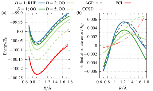
Figure 6: Potential energy curve (PEC) (left panel) and non-parallelity errors across the PEC (right panel) for HF with the cc-pVDZ basis. The non-parallelity errors are shifted absolute errors such that all PEC coincide at $R=0.9\,\mathrm{\textup{\AA}}$. The blue (green) curves denote the minimal matrix product state, MMPS, with restricted Hartree-Fock, RHF, ($D=1$ optimized) orbitals, where $D$ is the bond dimension. The dashed gray curve denotes the restricted antisymmetrized geminal product (AGP) curve. The dotted red curve corresponds to coupled cluster with singles and doubles (CCSD). The results are compared to the full configuration interaction reference (FCI; dashed red curve). For the MMPS computation, $\hat{P}=\hat{P}^{S_{z}}\hat{P}^{N}$ is used as the projector.

IV Conclusions

To summarize, we have explored a set of simple qualitative wavefunctions that we term minimal matrix product states (MMPS). We define the MMPS to be an MPS with small bond dimension of $D\sim 1$ combined with a projector onto the essential symmetries of the problem, e.g. particle, spin, and other symmetries. Already for $D=1$, this framework includes many other qualitative wavefunctions, such as symmetry broken and restored mean-field states, e.g. projected Hartree-Fock and antisymmetrized geminal power states, and further extends them, e.g. to beyond the seniority-zero sector in the case of the antisymmetrized geminal power. Importantly, it does so while retaining the same computational scaling for energy evaluation and optimization as with such states. This is because computations using the MMPS can use the density matrix renormalization group (DMRG) without relying on the generalizations of Wick’s theorem to incorporate symmetry projection. Similarly, the multisite version of the MMPS extends generalized valence bond and strongly-orthogonal geminal wavefunctions and other related ansätze beyond their product state structure, via symmetry breaking and projection, as well as for $D>1$.

We examined the behaviour of MMPS in a number of prototypical systems, namely H4, O2 and HF. The inclusion of the single creation operators is crucial to yield the observed improvements. In all cases we found that the MMPS ansatz even with $D=1$ gives correct qualitative behavior of the potential energy landscape, often significantly improving on the aforementioned ansätze. We also noted that orbital optimization, an essential ingredient also of the other methods, significantly improves the MMPS wavefunction. In the cases where we increased $D$ but still kept it “minimal” ($\leq 5$) we also observed a rapid improvement of the results.

We expect the MMPS ansatz to be useful in two main scenarios. First, MMPS could improve conventional DMRG calculations, which usually use large bond dimensions and do not invoke projectors to restore symmetry, by serving as an initial guess state to improve optimization. An example of this can be found in our previous work on spin-projected MPS,Li and Chan ; Li et al. (2019) which may be viewed through the lens of this work as a type of MMPS. Second, MMPS could serve as a method on its own for rapid exploration of the potential energy landscapes of molecular systems. This is especially useful for molecular dynamics simulations, where there is a great need for fast electronic structure calculations. Possible extensions to treat dynamical correlation Guo, Li, and Chan (2018a, b); Freitag et al. (2017); Guo et al. (2016); Hedegård et al. (2015); Pastorczak et al. (2019) and excited states Nakatani et al. (2014); Hu and Chan (2015); Dorando, Hachmann, and Chan (2007); Baiardi et al. (2019) are possible as well. Further, the methodology can straightforwardly be transferred to related domains, most importantly in applications to quantum dynamics.Lode et al. (2020); Weike and Manthe (2020); Larsson (2019); Leclerc and Carrington (2014)