Controlled imprisonment of wave packet and flat bands in a fractal geometry

Abstract

The explicit construction of non-dispersive flat band modes and the tunability of has been reported for a hierarchical 3-simplex fractal geometry. A single band tight-binding Hamiltonian defined for the deterministic self-similar non-translationally invariant network can give rise to a countably infinity of such self localized eigenstates for which the wave packet gets trapped inside a characteristic cluster of atomic sites. An analytical prescription to detect those dispersionless states has been demonstrated elaborately. The states are localized over clusters of increasing sizes, displaying the existence of a multitude of localization areas. The onset of localization can, in principle, be ‘delayed’ in space by an appropriate choice of the energy of the electron. The tunability of those states leads to the controlled decay of wave function envelope. The impact of perturbation on the bound states has also been discussed. The analogous wave guide model has also been discussed.

I Introduction

Flat band (FB) suther networks with the presence of one or more diffraction-free momentum independent flat energy band(s) have grabbed considerable attention over the recent few years dias -flach5 . On this ground, significant credit goes to the list of experimental realizations of these geometry sensible compact localized state (CLS) guzman -ram in a wide class of systems. For this challenging advancement in the fabrication technique, the topic has now extended its relevance beyond the condensed matter physics community - eventually it becomes a general field of discussion in optical nolte ; real ; seba , acoustic, phononic as well as polaritonic amo systems. The analogous macroscopic degeneracy associated with the FB physics lies at the heart of several novel physical phenomena which covers the formation of fractional quantum hall states kapit -ando as well as inverse Anderson Localization (AL) transition goda . Synthetic magnetic perturbation in optical networks yufan enables the destructive quantum interference resulting in a non-coherent eigenstate (CLS) bp2 -jin .

Destructive nature of wave interference resulted from the network due to the local geometric phase cancellation invites quantum confinement of wave function within the characteristic trapping island. Quantum transport properties is drastically affected for particles residing in a flat band. Hence the superposition of flat band modes exhibits non-diffrative dynamics of wave packet. Because of divergent effective mass tensor these states do not contribute to overall transmission leading to a singularity in the density of states profile for those non-resonant modes. There are several crucial factors hindering this morphology induced spatial imprisonment of excitation including the flatness of the band, finite lifetime of incoming particles and inter-particle interactions.

Recent study on ultracold fermionic atoms patterned into finite two dimensional optical lattices of a kagomé geometry has incorporated renewed interest in this field chern . Advancement in controlled growth of artificial, tailor-made lattices having atoms trapped in optical lattices with the complications of even a kagomé structure guzman ; tamura has contributed towards increasing interest in these deceptively simple looking systems. In the context of optics they are very much important as they lead to the long-distance advancement without any kind of distortion of shapes based on combinations of these flat modes. Actually all these bound states rely on a crucial wave interference condition. These contexts have been demonstrated and analyzed in photonic lattices mati ; real ; seba ; mati2 , graphene mele ; geim , superconductors deng ; kohno , fractional quantum Hall systems wen ; mudry ; gu , and exciton-polariton condensates amo . A fascinating feature of non-dispersive systems is the association of flat band modes to compact localized states (CLS) which reside on a finite cluster of the lattice and strictly die out elsewhere. The description of CLS has been experimentally cited in different flat band systems like frustrated magnets, and photonic crystal waveguides seba2 ; denz ; kle . There are a number of recent studies flach1 ; flach4 ; mielke2 that have discussed for flat band generating algorithms for giving a general prescription to identify the non-interacting Hamiltonian that supports CLS.

In this communication we study the existence of the self-localized modes and discuss the tunability aspect of those non-resonant modes for 3-simplex fractal acfrac geometry. Any fractal entity is readily different from the homogeneous Euclidean objects with respect to its peculiar dimensionality. An alternate demonstration of dimensionality is already mentioned by Hausdorff, named as “Hausdorff Dimension” where the log-log plot of two descriptors is termed as dimension vince . Also fractal geometries bp1 ; chacko have inherent scale invariance that can help us to find an analytical prescription to obtain countably infinity of such localized modes and the precise parametric control over those states. Before going to the specific analysis part we should expense few words about the motivational aspect details. It is needless to say that these fractal lattices have gained considerable momentum in the condensed matter community because of several application oriented scenario starting from stretchable electronics fan to transistors ieee , hydrogen storage ruiz , antennas nicola ; cohen , medical imaging nz and optimization model for stroke subtypes yeliz etc. Moreover, it is also reported that fractals may produce Hofstadter butterfly hof -smith and they are also suitable prototype example for showing fractional quantum Hall states pan , energy level splitting described via fractal dimensions auto and non-trivial quantum conductivity ac ; veen . Also, fractals are noticed in self assembled polymers bra . Although, fractal geometry does not have only theoretical point of interest, rather it has also been exploited experimentally to analyze the magneto-resistance gold1 , a distinct crossover of superconducting phase boundary gold2 . It has also been used to study the dimensional crossover and magneto-inductance measurement in Josephson junction arrays of periodically repeated Sierpinski gasket fractal network lee . Unlike the case of ideal deterministic fractal, experimentally fabricated systems cite the scale invariance solely at relatively shorter wavelength fluctuation limit, and it is seen that the degree of accuracy of the results is highly sensitive to the fractal or the homogeneous regimes which are being probed. This provides enough motivation to us to undertake a fractal type of lattice as our network of interest, but definitely with a slightly different objective.

The basic physical difference between the work related to Sierpinski gasket fractal atan (reported from our group) and the present $3$-simplex fractal lies in their spectral property. Sierpinski gasket fractal is seen to exhibit a set of hierarchical distribution of flat bands but in presence of external magnetic flux, we observed the clear disappearance of such bound states. The spectrum in presence of flux generates resonant bands populated by extended eigen functions. Whereas, in case of simplex fractal structure (present one) the analytical prediction shows that the self-localized states no longer vanish but an interesting tunability over the position of such states in respect of application of magnetic flux is demonstrated here. One can continuously modulate the flux, which is an external agency, to control those non-propagating modes. Our aim is to observe the dramatic effect of external parameter on the spectral density of states.

In this communication we have demonstrated an analytical scheme for a deterministic fractal entity to discern the localized states that are non-dispersive in nature. Controlled engineering of such states within the tight-binding framework has been discussed elaborately. It is needless to say that the scheme is in general applicable to several quasi-one dimensional model geometries. The proposition is exact and is consistent with the supportive numerical calculation. Here we observe that the position of the flat band may be tampered at will via selective parametric choice and the extent of localization can be manipulated using the self similar pattern of the structure. That means selectively we can block a particular wave train of definite energy using symmetry partitioning and related interference effect and one can easily predict the area of localization from the scale of length used. Real space renormalization group method (RSRG) have been employed to see the multifractal distribution of flat band modes. Since the fractal does not possess any sort of translational ordering, only straightforward diagonalization of the Hamiltonian may not provide the complete spectral information related to FB modes. There is probability that few modes may be slipped away from the original spectrum (in the thermodynamic limit) when one goes for the change in scale of length due to the Cantor-set ali like fragmented spectrum. The method followed here could help in this regard and provide an analytically exact description of FB states for such quasi-one dimensional fractal network. The impact of applying uniform magnetic perturbation is also discussed in terms of the band dispersion. The non-trivial position sensitivity on external parameter makes the discussion challenging to the experimentalists. Actually, all these analytical results will have physical implication, specially when people go for direct experimental visualization of localization and other related properties in low dimensional lattices, and hence this discussion may inspire further experiments on grafted lattices in low dimensions. In view of this, the analogous optical context has been discussed in Sec. VII along with the proposition of single mode wave guide model. The equivalent monomode wave guide model is proposed to establish the equivalence of the photonic localization with the same spirit as that in the electronic case.

We thus summarize the complete analysis. In Sec. II, we first describe the model system and the Hamiltonian. Then Sec. III discusses the basic analytical scheme to obtain the whole hierarchy of the self-localized states and the idea of expansion of the extent of characteristic island. Sec. IV contains usual computation of density of states describing the allowed eigenspectrum. along with the discussion of band dispersion. After that in Sec. V we have demonstrated the impact of uniform magnetic flux on the flat band modes. Sec. VI discusses the experimental possibilities, Sec. VII demonstrates an equivalent optical wave guide model and finally in Sec. VIII we conclude our results.

II Model system and Hamiltonian

We start our demonstration by referring the Fig. 1 where a finite segment of a geometrically frustrated $3$-simplex fractal network and its growth sequel are shown pictorially. The quasi-one dimensional hierarchical geometry has

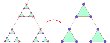
Figure 1: (Color online) Schematic representation of the part of an infinite hierarchical $3$-simplex fractal geometry (left) and renormalized version of the original network (right). The sites marked by red dotted circle are left after one step renormalization.

an inherent self-similar pattern and that leads to an exotic spectral canvas. In the tight-binding language, the overlap parameter between the nearest neighboring atomic sites only is considered in this model. One can easily describe the entire system by the standard Hamiltonian acfrac ; atan written in the Wannier basis, viz.,

$$H=\sum_{n}c_{n}^{\dagger}\epsilon_{n}c_{n}+\sum_{\langle nm\rangle}[c_{n}^{\dagger}t_{nm}c_{m}+h.c.]$$ (1)

The potentials of all the atomic sites are considered to be identical (equal to $\epsilon$) but the hopping integrals are different. The connectivity along the arm of each elemental triangular plaquette is taken as $t$ and one such plaquette is coupled with the other plaquette by the overlap integral $\tau=xt$; $x$ being the coupling parameter. This coupling factor brings the off-diagonal anisotropy. However, our main objective or point of interest is to see the topological aspects of spectral landscape with the variation of inter-plaquette coupling strength $x$. It is needless to say that the results are no longer sensitive to the numerical values of the parameters of the Hamiltonian. Since we will concentrate on the localization issue induced by the description of the network, we assume, without any loss of generality $\epsilon=0$, $t=1$ for numerical calculation. The tight-binding difference equation boy (an alternate form of Schrödinger’s equation), viz.,

$$(E-\epsilon_{j})\psi_{j}=\sum_{k}t_{jk}\psi_{k}$$ (2)

allows us to analyze the tunability of trapping of electronic wave functions with respect to the modulation of anisotropy parameter $x$.

Following the real space renormalization group (RSRG) scheme, an appropriate subset of the entire lattice can be easily decimated out in terms of the amplitudes of the ‘surviving’ nodes to generate the scaled version of the fractal and this can be done by the use of difference equation. In this procedure the parameters of the Hamiltonian may be renormalized as follows,

$$\epsilon(n+1) = \epsilon(n)+\frac{2t^{2}(n)\mathcal{D}_{2}(n)}{\mathcal{D}_{3}(n)}$$

$$t(n+1) = \frac{t^{2}(n)T(n)\left[t(n)+\mathcal{D}_{1}(n)\right]}{\mathcal{D}_{3}(n)}$$

$$T(n+1) = T(n)$$ (3)

where $\mathcal{D}_{1}(n)=[E-\epsilon(n)-T(n)]$, $\mathcal{D}_{2}(n)=\mathcal{D}_{1}(n)[E-\epsilon(n)]-t^{2}(n)$ and $\mathcal{D}_{3}(n)=\mathcal{D}_{2}(n)[E-\epsilon(n)-t(n)]-T^{2}(n)\mathcal{D}_{1}(n)$. Here $n\geq 0$ denotes the stage of renormalization. All the recursion relations in Eq. (3) can now be exploited for explicit analytical construction and demonstration of a set of compact localized states in such deterministic fractal geometry. These equations will also help us to find out the expected hierarchical distribution of compact localized modes, if any.

III Analytical construction of flat band state

III.1 The basic scheme

One can easily check that by employing the difference equation, if we set

$$E=\epsilon-t(x+1)$$ (4)

a consistent solution can be achieved for which the non-vanishing amplitudes are concentrated

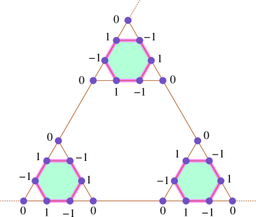
Figure 2: (Color online) Wave function amplitude configuration for the compact localized state at $E=\epsilon-t(x+1)$ is shown pictorially. Each of the shaded hexagonal clusters of atomic sites describes the characteristic trapping island and the connecting nodes with zero amplitudes makes the kinetic information quenched within the finite size clusters.

along the peripheral nodes of the characteristic trapping cell (hexagonal plaquette here). The connecting node in between any two such clusters has zero wave function amplitude as shown in the Fig. 2. By making the amplitude vanish at the selective quantum dot locations, it is possible to confine the mobility of the injected wave train (corresponding to the above-mentioned particular value of energy) within a cluster of atomic sites of finite area. The phase decoherence makes the prisoner trapped inside the characteristic island. Since the dynamics of the wave packet gets locked in space, the analytical construction of those self-localized modes resembles the essence of a molecular state egg . It is needless to say that the eigenstate is spatially localized due to the formation of physical barrier constituting the sites with zero wave function amplitudes. The destructive quantum interference leads to divergent effective mass tensor and the immobility of the particle. Several clusters are distributed throughout the infinite lattice and one such island is effectively decoupled from the another one making the excitation trapped inside it. The wave function associated with this eigenmode does not have any overlap with that described on the neighboring hexagonal plaquette.

III.2 Self similarity: Flat band hierarchy

The underlying fractal geometry bears a self-similar growth sequence.

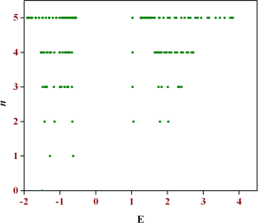
Figure 3: (Color online) Hierarchical distribution of localized modes with the index of renormalization (equivalently the scale of length). The roots form a countably infinite set in the thermodynamic limit.

This scale invariance of the structure can be used to construct self trapped wave functions at any desirable step of hierarchy. The analogous localization area of such bound states can be adjusted at will by a justified choice of RSRG index. This is because of the fact that the corresponding eigenvalues can be computed using the following eigenvalue equation for any arbitrary value of $n$, viz.,

$$E=\epsilon(n)-(x+1)t(n)$$ (5)

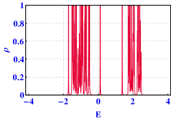
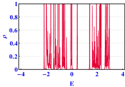
(a) (b) (c)

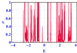
Figure 4: (Color online) Plot of density of eigenstates $\rho(E)$ against the energy $E$ of the electron for (a) $x=0.5$, (b) $x=1.0$ and (c) $x=1.5$ respectively. The anisotropic parameter $x$ sets the range of the band extent.The flat bands correspond to sharp spikes at (a) $E=-1.5$, (b) $E=-2$ and (c) $E=-2.5$ respectively. The position of the self-localized state is sensitive to the anisotropy index $x$. We have set $\epsilon=0$ and $t=1$ for computational analysis part.

From the above equation we see that the localized modes will be an obvious function of the anisotropy parameter $x$. Hence the position of these non-coherent bound modes is sensitive on the choice of the parameter $x$ and thus provides a non-trivial selectivity. This is expected. The energy eigenvalues obtained from the Eq. (5) for different stage of hierarchy are plotted in Fig. 3. In this demonstration we have particularly set the off-diagonal ansiotropy parameter $x$ as $0.5$. It is seen that as the iteration index increases the number of those self-localized non-resonant modes increases accordingly. The distribution of modes exhibits a typical cantor set-like fragmented spectral sketch which basically reflects the spectral nature of the fractal network. We can safely comment that finally in the thermodynamic limit ($N\rightarrow\infty$) such roots will densely fill up the entire canvas. The sequential clustering of eigenmodes with renormalization index is distinctly cited in Fig. 3. It is needless to say that all these states will carry the non-dispersive signature in the overall band spectrum due to the low group velocity of the wave packet. However we will present logical justification in support of this statement in the subsequent discussion. Now it is to be emphasized that the definite analytical prescription of flat band hierarchy is made possible with the aid of RSRG method only. In this non-translationally invariant lattice, the scheme therefore provides an analytically exact description of at least a subsection of the entire spectrum. Here is the strength of our analytical attempt. Another interesting scenario related to the nature of localization can be demonstrated as follows.

III.3 Extension of quantum prison: Staggered localization

For any energy eigenvalue obtained from any $n$-th level of hierarchy of the underlying fractal geometry, say, $n=l$, the hopping integral remains non-vanishing up to that particular $l$-th stage and starts decaying beyond it ($n>l$). This signifies that the associated electronic wave functions between the nearest neighboring atomic sites have the non-vanishing overlap at that length scale, When mapped back on to the original fractal network, it definitely amounts to a non-zero overlap of the wave function between the sites much beyond the nearest neighbors (for $n>1$). That is, the localization of wave packet is based on a cluster of quantum dots, not pinned at any particular node. Such clusters are distributed throughout the geometry, but effectively disconnected from each other, Therefore, the confinement of wave train is delayed in space. The effect is named as staggered localization leading to the creation of a whole set of compact localized states. The spatial extent of the characteristic unit cell depends only on the iteration index. It is seen that the localization area grows hierarchically with the sequential increment of $n$.

IV Spectral landscape

IV.1 Computation of density of states

Before making any comment on the dispersionless character of the states constructed so far, we proceed to acquire a general idea of the overall spectrum that describes the entire landscape of allowed eigenmodes as a function of the energy of the injected projectile. It is clear from the Eq. (4) that for each value of the flat band energies arising out from the equation, for any arbitrary value of the coupling strength, it should give a sharp distinct spike in the density of states (DOS) spectrum. This is due to the expected singularity coming from the zero mobility of the wave train corresponding to those specific bound states and is governed by the following equation,

$$\rho\propto\int v_{g}^{-1}dk$$ (6)

Due to the destructive wave interference the wave packet corresponding to such self-localized modes gets trapped inside the characteristic trapping prison. Hence the group velocity $v_{g}$ attains a vanishingly small value ($v_{g}\rightarrow 0$). The immediate consequence of immobility is the spectral divergence and this turns out to be an important predetermining factor in the anomalous behavior of transport, if any. From the above density of modes plots (Fig. 4) this singular nature corresponding to the FB modes is apparent.

The system is a fractal object that carries an inherent scale-invariance. Complete absence of translational periodicity makes the appearance of non-resonant localized eigenstates an obvious phenomenon. Hence the fragmented kind of cantor set-like spectral pattern is followed from the self-similarity present in the underlying structure. One can follow the standard procedure to compute the electronic density of states by virtue of the well-used relation eco , viz.,

$$\rho(E)=-\left(\frac{1}{N\pi}\right)Im[TrG(E)]$$ (7)

Here $G(E)=[E-H+i\Delta]^{-1}$ is the usual green’s function and $\Delta$ is the imaginary part of the energy, comparably small enough, added for the numerical evaluation of DOS. $N$ denotes the system size and ‘Tr’ is the trace of the greens’ function. Throughout the numerical analysis, we have set $\epsilon=0$ and $t=1$. In Fig. 4(a)-(c) we have presented the typical density of states patterns respectively for $x=0.5$,$1.0$ and $1.5$ as a function of the energy for the quasi-one dimensional hierarchical geometry. For small value of the anisotropy parameter $x$ (here $x=0.5$), it cites several distinct spikes and very few thin subbands as expected for a fractal entity reflecting its clear distinction from any homogeneous Eucledian objects. The spectrum consists of a number of localized modes distinctly separated by gaps (disallowed modes). For any of the energy eigenvalue among any of the discrete spikes, the hopping integral starts diminishing after finite number of loops and this confirms the localization. The dynamics of the electrons has an intricate relationship with the geometric configuration of the underlying fractal lattice. The hopping is the off diagonal element of the Hamiltonian between the Wannier orbitals at neighboring sites, its vanishing clearly demands that the corresponding electronic wave function cannot extend beyond a certain cluster of minimal dimension. In other words, there is no overlap between the wave functions beyond a plaquette of certain size. Thus, the amplitudes of the wave function get trapped in local islands, the islands being distributed and decoupled from each other all over the fractal geometry. With the gradual increase in the strength $x$, we observe the formation of few mini-patches of allowed energies. However, it retains its multifractal character of the spectrum with the existence of non-resonant states.

The features of flat band modes can be easily characterized from the portrait of density of states (DOS) in the tight-binding prescription. For each of the FB eigenmodes, the non-zero wave function amplitudes are distributed over a finite size atomic cluster and those trapping cells accommodating the non-trivial distribution of wave functions get isolated from each other beyond a certain scale. The corresponding hopping integral shows decaying behavior with the progress of iteration loops (scale of length) and this confirms the localization of the associated wave packet corresponding to such self-localized states.

IV.2 Eigenspectrum as a function of anisotropy parameter

To complete the discussion we now examine the effect of anisotropy index $x$. For this, we have presented an

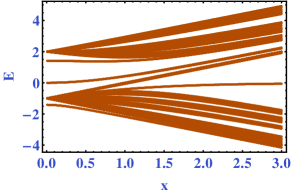
Figure 5: (Color online) Allowed eigenspectrum as a function of anisotropy parameter $x$ for a finite size of the fractal system.

allowed eigenvalue distrbution of a $5$-th generation of fractal as a function of $x$ in the Fig. 5. With the modulation of the parameter $x$, the overlap integral in between any two basic triangular plaquettes changes accordingly. This has an obvious impact on the spectral distribution as seen in the Fig. 5. The gradual enhancement of anisotropy parameter leads to the formation of several allowed minibands and few selective band overlap. Bandgap is also visible showing the window of disallowed modes. The density of allowed modes is seen to increase with $x$. This is expected because increase in $x$ resonates the inter-plaquette connectivity. We can safely comment that the density of states is larger in the regime $t\leq x\leq 3t$ and this tradition is expected to continue beyond this range ($x\geq 3t$) exhibiting more number of band merging. This non-trivial variation with $x$ provides a tunability of those self-localized states that could be interesting from the experimental point of view.

IV.3 Band dispersion

The underlying geometry does not have any translational ordering and hence the deduction of energy-momentum

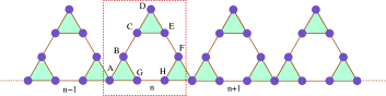
Figure 6: (Color online) Schematic representation of the periodic array of fractal geometry of first generation.

relationship in usual tight-binding language is no longer possible. This prompts us to undertake an indirect but effective way to discern the non-dispersive flavor of the whole hierarchy of those self-localized states. The motivation behind this analysis is that the compact localized states constructed in the earlier section display a typical self-localization induced by the nature of the resultant wave interference. The trapping of amplitudes inside the allowed zone makes the particle ‘super-heavy’ (infinite effective mass) such that it loses its mobility. This immediately offers vanishing band curvature corresponding to the particular eigenmode and hence carries a non-dispersive signal.

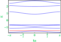
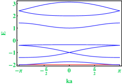
(a) (b) (c)

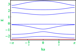
Figure 7: (Color online) Energy-momentum relationship plotted for a quasi-one dimensional array of simplex fractal geometry of first generation for (a) $x=0.5$, (b) $x=1.0$ and (c) $x=1.5$ respectively. The red line in each case denotes the corresponding non-dispersive flat band satisfying the eigenvalue equation (Eq. (4)). The number of bands will increase sequentially with the level of hierarchy.

We choose a periodic array as depicted in Fig. 6 by considering a finite generation of simplex fractal as unit cell. For this array, we can recast the Hamiltonian in the momentum space bp1 , viz.,

$$H=\sum_{k}\psi^{\dagger}_{k}\mathcal{H}(\bm{k})\psi_{k}$$ (8)

This typical construction creates a top vertex with coordination number equal to two. Though it was not present in the infinite geometry where we cannot see the ends, but when we will upgrade the generation of the fractal, in the true thermodynamic limit, this will act as a reasonably good approximant and carry the flavor of the original system. Our ultimate goal is to prove the dispersionless nature of the compact localized modes for this geometrically frustrated fractal entity. Therefore it is expected that in the language of reciprocal space, the momentum insensitive part of the band dispersion should produce the same bound states. By the conversion, Hamiltonian matrix reads as,

$$\mathcal{H}(\bm{k})=\left[\begin{array}[]{cccccccc}\epsilon_{A}&t&0&0&0&te^{-ik}&t&te^{-ik}\\ t&\epsilon_{B}&xt&0&0&0&t&0\\ 0&xt&\epsilon_{C}&t&t&0&0&0\\ 0&0&t&\epsilon_{D}&t&0&0&0\\ 0&0&t&t&\epsilon_{E}&xt&0&0\\ te^{ik}&0&0&0&xt&\epsilon_{F}&0&t\\ t&t&0&0&0&0&\epsilon_{G}&xt\\ te^{ik}&0&0&0&0&t&xt&\epsilon_{H}\end{array}\right]$$ (9)

We have set identical potentials for all the sites and carried out the dispersion equation. For this quasi-one dimensional fractal structure we have plotted the band dispersion relation by virtue of the above matrix (in reciprocal space) for different values of $x$ as cited in the Fig. 7. Here we find that the band dispersion curves readily confirms the dispersionless behavior of the analytically constructed self localized states. The red lines in all the cases show the flat bands satisfying the analytical prescription (Eq. (4)). Even with a modest unit cell combination for the array, the staggered localized states corresponding to

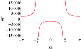
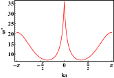
(a) (b)
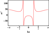
(c) (d)

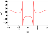
Figure 8: (Color online) Effective mass variation for the fractal geometry for (a) $x=0.05$, (b) $x=0.5$, (c) $x=1$ and (d) $x=2$ respectively.

the truly infinite system are showing up. The plots exhibit other dispersive bands and quasi-dispersive (bands with extremely low but non-zero curvature). For the later case, the electrons carrying those particular energies have significantly low mobility. Also it is observed that in absence of asymmetry ($x=1$), there is a band crossing which is seen to be missing in the next plot ($x=1.5$) and thus it immediately creates an energy gap in between the two bands with the increment of anisotropy index. It is needless to say that the number of bands (both dispersive and non-dispersive) will increase sequentially with the increase in hierarchy and all those modes will densely fill up the band structure. Also all the localized modes will form a set of hierarchy comprising of countably infinite number of such modes in the thermodynamic limit. This message is clear from the Fig. 3 and the associated discussion.

IV.4 Parameter selective control of effective mass

From the band dispersion plot we see the existence of some dispersive states. Of course the position is highly sensitive on the value of anisotropy parameter $x$. Hence using that factor one may tune the group velocity of the wave packet as well as the band curvature (equivalently effective mass tensor of the particle). Thus parameter induced engineering of effective mass essentially invites the precise control over mobility of the incoming projectile. Fig. 8 represents the variation of effective mass for different strength of the coupling parameter for one such resonant mode. From the plots we see that for low enough value of $x$, the effective mass of the particle shows extremely large magnitude and hence the group velocity becomes considerably small. This leads to localization of wave train. With the gradual increment magnitude of effective mass tends to reach some finite values, but still the variation is oscillating in nature between both positive and negative ranges. When the off-diagonal anisotropy is absent ($x=1$) oscillation is seen to be restricted within some positive finite value and again for moderate or strong enough anisotropy index ($x>1$), again the sign flipping scenario comes back within finite range of values. Also we observe several diverging behavior of mass for few k-points. Another interesting fact is the re-entrant fashion from positive to negative regime through those singular points. The parameter selective sharp cross-over between the hole like and electron like character of the particle is the main physical implication of this discussion. One may tune the electron-lattice interaction with the choice of system parameter.

V Impact of perturbation on flat band

V.1 Flux sensitive Aharonov-Bohm caging

In the previous section, we have discussed the effect of off-diagonal anisotropy on the band dispersion. Now we will switch off this anisotropy effect and make the hopping uniform everywhere. The central aim of the subsequent discussion is to study the sustainability of the FB in presence of homogeneous magnetic perturbation piercing through any local closed plaquette of the geometry. All the flat band states carry macroscopic degeneracy with a basis of eigenstates which are spatially localized since the analogous wave function form a standing-wave pattern because of the incoherent wave interference. This extensive degeneracy imports an obvious sensitivity to many kinds of external perturbation, including disorder (deterministic or random), different types of interactions or external fields. Based on the response to these kind of external parameter, a clear distinction is obtained by Aoki et al. to classify the FB networks ando . Uniform magnetic field breaks the macroscopic degeneracy; destroys the FB in Mielke’s and Tasaki’s lattices mielke -tasaki and transforms it into a pattern of Hofstadter butterfly. On the contrary, Lieb or Dice class of networks support chiral FB flach1 which do not respond to the external agency of perturbation due to the symmetry protection. Because this sustainability involves “local symmetry” of the sub-lattice connection. The later class of superlattices exhibiting symmetry-protected chiral flat dispersionless band was first cited by Aoki et al. shima . The undisturbed FB state protect their extensive degeneracy, though there may be position shifting with respect to the application of magnetic field. This topic has gained considerable interest since $2012$ lan ; zhu . Also we should mention that the flux dependent flat band is a subset of a widely known phenomena, i.e., Aharonov-Bohm caging vidal and has been recently verified experimentally by a group of workers sebanew .

In our geometrically frustrated fractal system, the uniform magnetic flux is trapped inside each basic hexagonal plaquette and this eventually breaks the time reversal symmetry (at least locally) of the off-diagonal element of Hamiltonian along the bond. The incorporation of magnetic flux $\Phi$ introduces Peierls’ phase factor associated with the overlap parameter, viz., $t\rightarrow te^{i\Theta}$, where $\Theta=(\pi\Phi/3\Phi_{0})$, $\Phi_{0}=hc/e$ is known as fundamental flux quantum. It is to be noted that to see the effect of applying perturbation, we set $x=1$. Therefore the hopping integral is uniform magnitude-wise everywhere in lattice. Now we

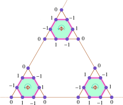
Figure 9: (Color online) Amplitude distribution for flux sensible flat band at $E=\epsilon-2t\cos\Theta$. The macroscopic degeneracy associated with the flat bands is sustained in presence of perturbation. We have set the anisotropy index $x=1$ to see the flux tunability of flat bands.

switch on the magnetic perturbation $\Phi$. By virtue of the difference equation it is quite trivial to check that if we take $E=\epsilon-2t\cos\Theta$, then a flux dependent amplitude configuration can be drawn

(a)
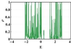
(b)

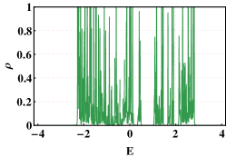
Figure 10: (Color online) Variation of density of states $\rho(E)$ as a function of the energy $E$ of the incoming electron for $x=1$. The magnetic flux threading each elemental triangular plaquette is set at (a) $\Phi=\Phi_{0}/4$ and (b) $\Phi=\Phi_{0}/2$ respectively. $\Phi_{0}=hc/e$ is the fundamental flux quantum.

satisfying the difference equation and is shown in Fig. 9. The resultant nature of the quantum interference obtained from multiple quantum dots solely determines the sustainability issue of the FB modes. From the above equation it is clear that with the application of homogeneous magnetic flux, the position of the FB is now extremely sensitive to the applied flux. Hence one can tune the external parameter at will to trap any particular wave packet of definite energy eigenvalue in a selective way. This means for the injected projectiles to be locked via lattice structure the energy must have to satisfy the above eigenvalue equation for a particular value of flux. The position engineering controlled by the periodic modulation of flux makes this discussion interesting from the experimental perspective. Another point is that the above flux involved amplitude distribution scenario is valid for any finite value of flux. Therefore, one can say the extensive degeneracy associated with the FB states is not disturbed anyway by the application of flux. In Fig. 10 we have shown the density of eigenstates plots for two different values of magnetic flux $\Phi=\Phi_{0}/4$ and $\Phi_{0}/2$ respectively. It is needless to mention that owing to the vanishing mobility of the wave train corresponding to FB mode, the DOS presents a distinct divergent behavior for the selective states satisfying the flux-dependent equation. This singularity confirms the prediction of flux modulated flat band states. Of course, this singularity is now external agency dependent.

V.2 Allowed eigenspectrum

For the sake of completeness we should present a distribution showing the allowed eigenmodes as a function of external magnetic flux (Fig. 11). This figure also supports the existence of flux tunable flat band.

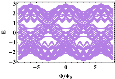
Figure 11: (Color online) Flux sensitive allowed eigenspectrum as a function of external perturbation. The spectrum is flux periodic with periodicity equal to one flux quantum. We have set the anisotropy index $x=1$ to see the flux tunability of flat bands. The flux tunable flat band at $E=\epsilon-2t\cos\Theta$ is seen to be present.

This diagram may be considered an analogous dispersion relation because for an electron moving round a closed path, it is well known that the magnetic flux plays the similar physical role as that of the wave vector gefen . The eigenmodes create miniband-like structure as a function of external flux. The pattern presented contains an inherent periodicity equal to six times the fundamental flux quantum $\Phi_{0}$. First of all, the eigenspectrum supports the existence of flux sensitive flat band modes as suggested in Fig. 9. One can continuously engineer the magnetic flux to adjust the imprisonment of wave train with high selectivity. Moreover, there are a number of inter-twined band overlap, and a quite densely packed distribution of allowed modes, forming quasi-continuous flux-periodic $E-\Phi$ band structure. Close observation of this eigenspectrum reveals the formation of interesting variants of the Hofstadter butterflies hof . The spectral landscape is a quantum fractal, and encoding the gaps with appropriate topological quantum numbers remains an open problem for such deterministic fractals.

VI Discussion regarding experimental aspects

The essence of quantum imprisonment of incoming wave packet by means of lattice geometry and wave interference resulted from the network is no longer a theoretical issue in the present era of advanced nanotechnology and lithography techniques. Thanks to the experimentalists that they have made it possible to visualize the authentic scenario related to the localization of injected messenger in laboratory with the help of femto second laser-writing procedure and optical induction technique. Consequently, the engineering of localization of wave train is a very common aspect in the different topics of condensed matter physics. Also it is very pertinent in case of classical electromagnetic signal and light as well. The experimental progress started with Yablonovitch yab1 ; yab2 along with the propositions from John john and Pendry and MacKinon pend related to the realistic experimental observation of Anderson localization. This essentially invites the path-breaking idea of slow light engineering baba that opens up the possibility of spatial compression of light energy. This area of research has also enriched by the most recent examples seba ; seba2 ; sebanew of photonic localization hu ; hu2 in some one or two dimensional geometries. This gives a scope for direct observation of diffraction free FB states. All these challenging experiments have become the milestone in this field of study and it is needless to say that these inspire us to take such model fractal object as our system of interest. The predictability of the flat band engineering with respect to the anisotropy index and magnetic flux as well, throws an achievable challenge to the experimentalists to test the analytical result with proper modulation. This may be possible in accordance with the proposition of S. Longhi longhi1 ; longhi2 , where it was shown that the introduction of the concept of flux controlled band engineering may be possible as a synthetic gauge field may be fabricated by changing the propagation constant and this could help in the experimental possibility.

VII Proposed optical wave guide model

Exact analogy between the electronic case and the associated optical scenario within the tight-binding formalism is very useful as well as pertinent aspect. The concept was first initiated by Sheng et al. alexan ; sheng , where they showed that the propagation of wave train through any quasi-one dimensional monomode wave guide structure has a direct correspondence with the same electronic model with proper initial conditions.

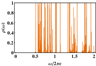
Figure 12: (Color online) Representation of density of photonic modes as a function of the frequency of the incoming wave. Frequency $\omega$ is taken in unit of $2\pi c/a$, $a$ being the wave guide dimension.

The analogy of the solution of the wave equation with the difference equation for an electron moving in an identical geometry provides a parallel platform to study the localization issue of classical waves. Also, it is needless to say that the one-to-one mapping is completely a mathematical artifact and once that is done the recursion relations exploited for RSRG approach become insensitive to whether the input appears from a quantum background or a classical one. We should point out that the propagation of signal can be adjusted and controlled by appropriate selection of dielectric parameter of the core material. If we consider a definite dimension of the wave guide segment from the very beginning, then it is quite trivial to obtain the frequency of incoming wave packet corresponding to the localized modes.

Following Sheng et al., one can fabricate a single channel wave guide model formed by the segments having the same dimensions arranged in a simplex fractal geometry. Within the tight-binding framework we have plotted (Fig. 12) the variation of density of optical modes against the frequency $\omega$ of the incoming wave to acquire knowledge about the general idea about the allowed eigenmodes for the analogous fractal wave guide network. The distribution of optical modes within the frequency regime $0<\omega<2$ shows several clusters of non-zero values of density of photonic modes. The numerical value of the dielectric constant $\epsilon_{r}$ is arbitrarily set as $2$ and the anisotropy in the hopping (as discussed in the electronic case) is introduced by incorporating a wave guide segment of same dimension but with different dielectric parameter ($\epsilon_{r}=3$) in the suitable place. The spectrum is highly fragmented in character and this is expected for a fractal structure. The appearance of localized modes triggered by destructive wave interference is clear in the graphical presentation. Also, the density of modes spectrum exhibits few gaps in the frequency range for which the wave propagation is not permissible. Hence this proposed model may act as an appropriate candidate for photonic bandgap (PBG) yab1 ; yab2 kind of system.

VIII Summary and outlook

We have described the analytical scheme following real space renormalization group technique to compute the hierarchical distribution of dispersionless flat band eigenmodes for geometrically frustrated kind of $3$-simplex fractal lattice. These states are essentially localized over clusters of atomic sites by means of phase cancellation at some connecting nodes induced by destructive wave interefrence. The extent of imprisonment of wave packet may be controlled at will via selective choice of iteration index (or scale of length). The prescription presented here provides an exact set of countably infinite number of bound states as a function of off-diagonal anisotropy parameter. The numerical evaluation of density of eigenstates and band dispersion corroborate our analytical proposition. The impact of applying uniform magnetic perturbation is discussed elaborately. Flux tunable position sensitive macroscopically degenerate flat bands are seen in this fractal geometry. Continuous periodic modulation of external flux over the non-resonant modes eventually invites flux sensitive localization for this type of quasi-one dimensional network. The inherent singularity corresponding to those modes is also seen to be present in the spectral landscape. Hierarchical distribution of flat band modes in the thermodynamic limit is basically compatible with the fragmented nature of eigenspectrum.

- (1) B. Sutherland, Phys. Rev. B 34, 5208 (1986).
- (2) R.G. Dias, J.D. Gouveia, Sci. Rep. 5 16852 (2015).
- (3) M. Hyrkäs, V. Apaja, M. Manninen, Phys. Rev. A 87, 023614 (2013).
- (4) L. Morales-Inostroza, R.A. Vicencio, Phys. Rev. A 94, 043831 (2016).
- (5) A. Ramachandran, A. Andreanov, S. Flach, Phys. Rev. B 96, 161104(R) (2017).
- (6) S. Flach, D. Leykam, J. D. Bodyfelt, P. Matthies, A. S. Desyatnikov, Europhys. Lett. 105, 30001 (2014).
- (7) J. D. Bodyfelt, D. Leykam, C. Danieli, X. Yu, S. Flach, Phys. Rev. Lett. 113, 236403 (2014).
- (8) W. Maimaiti, A. Andreanov, H. C. Park, O. Gendelman, S. Flach, Phys. Rev. B 95, 115135 (2017).
- (9) D. Leykam, A. Andreanov, S. Flach, Adv. Phys. X 3, 1473052 (2018).
- (10) G.-B. Jo, J. Guzman, C. K. Thomas, P. Hosur, A. Vishwanath, and D. M. Stamper-Ku, Phys. Rev. Lett. 108, 045305 (2012).
- (11) D. Guzman-Silva, C. Meja-Cortes, M. A. Bandres, M. C. Rechtsman, S. Weimann, S. Nolte, M. Segev, A. Szameit, and R. A. Vicencio, New J. Phys. 16, 063061 (2014).
- (12) S. Taie, H. Ozawa, T. Ichinose, T. Nishio, S. Nakajima, and Y. Takahashi, Sci. Adv. 1, e1500854 (2015).
- (13) R. A. Vicencio, C. Cantillano, L. Morales-Inostroza, B. Real, C. Mejía-Cortès, S. Weimann, A. Szameit, and M. I. Molina, Phys. Rev. Lett. 114, 245503 (2015).
- (14) S. Mukherjee, A. Spracklen, D. Choudhury, N. Goldman, P. Öhberg, E. Andersson, and R. R. Thomson, Phys. Rev. Lett. 114, 245504 (2015).
- (15) F. Baboux, L. Ge, T. Jacqmin, M. Biondi, E. Galopin, A. Lemaître, L. Le Gratiet, I. Sagnes, S. Schmidt, H. E. Treci, A. Amo, and J. Bloch, Phys. Rev. Lett. 116, 066402 (2016).
- (16) M. R. Slot, T. S. Gardenier, P. H. Jacobse, G. C. P. van Miert, S. N. Kempkes, S. J. M. Zevenhuizen, C. Morais Smith, D. Vanmaekelbergh, I. Swart, Nature Phys. 13, 672 (2017).
- (17) S. Mukherjee and R. R. Thomson, Opt. Lett. 40, 5443 (2015).
- (18) S. Xia, A. Ramachandran, S. Xia, D. Li, X. Liu, L. Tang, Y. Hu, D. Song, J. Xu, D. Leykam, S. Flach, and Z. Chen, Phys. Rev. Lett. 121, 263902 (2018).
- (19) E. Kapit, E. Mueller, Phys. Rev. Lett. 105, 215303 (2010).
- (20) E. Tang, J.-W. Mei, X.-G. Wen, Phys. Rev. Lett. 106, 236802 (2011).
- (21) K. Sun, Z. Gu, H. Katsura, S. Das Sarma, Phys. Rev. Lett. 106, 236803 (2011).
- (22) T. Neupert, L. Santos, C. Chamon, C. Mudry, Phys. Rev. Lett. 106, 236804 (2011).
- (23) W.-F. Tsai, C. Fang, H. Yao and J. Hu, New J. Phys. 17, 055016 (2015).
- (24) H. Aoki, M. Ando and H. Matsumura, Phys. Rev. B 54, R17296 (1996).
- (25) M. Goda, S. Nishino, H. Matsuda, Phys. Rev. Lett. 96, 126401 (2006).
- (26) Z. Yu and S. Fan, Nat. Photonics 3, 91 (2009).
- (27) B. Pal, Phys. Rev. B 98, 245116 (2018).
- (28) A. Bhattacharya and B. Pal, Phys. Rev. B 100, 235145 (2019).
- (29) S. M. Zhang and L. Jin, Phys. Rev. A 100, 043808 (2019) and the references therein.
- (30) G.-W. Chern, C.-C. Chien and M. Di Ventra, Phys. Rev. A 90, 013609 (2014).
- (31) K. Shiraishi, H. Tamura, and H. Takayanagi, Appl. Phys. Lett. 78, 3702 (2001).
- (32) V. Apaja,M. Hyrkäs, and M. Manninen, Phys. Rev. A 82, 041402(R) (2010).
- (33) C. L. Kane and E. J. Mele, Phys. Rev. Lett. 78, 1932 (1997).
- (34) F. Guinea, M. I. Katsnelson, and A. K. Geim, Nat. Phys. 6, 30 (2010).
- (35) S. Deng, A. Simon, and J. Köhler, J. Solid State Chem. 176, 412 (2003).
- (36) M. Imada and M. Kohno, Phys. Rev. Lett. 84, 143 (2000).
- (37) S. Yang, Z.-C. Gu, K. Sun, and S. Das Sarma, Phys. Rev. B 86, 241112 (2012).
- (38) E. Travkin, F. Diebel, and C. Denz, Appl. Phys. Lett. 111, 011104 (2017).
- (39) S. Klembt, T. H. Harder, O. A. Egorov, K. Winkler, H. Suchomel, J. Beierlein, M. Emmerling, C. Schneider, and S. Höfling, Appl. Phys. Lett. 111, 231102 (2017).
- (40) A. Mielke, J. Phys. A: Math. and Gen. 24, 3311 (1991).
- (41) A. Chakrabarti, Phys. Rev. B 72, 134207 (2005).
- (42) J. Keesling, P. Duvall, and A. Vince, J. London Math. Soc., 61 (3):748-760, (2000).
- (43) B. Pal and K. Saha, Phys. Rev. B 97, 195101 (2018).
- (44) M. Ghadiyali and S. Chacko, arXiv.: 1904.11862 (2019).
- (45) J. A. Fan, W.-H. Yeo, Y. Su, Y. Hattori, W. Lee, S.-Y. Jung, Y. Zhang, Z. Liu, H. Cheng, L.o Falgout, M. Bajema, T. Coleman, D. Gregoire, R. J. Larsen, Y. Huang, and J. A. Rogers, Nat. Comm. 5, 3266 (2014).
- (46) R. Reiner, P. Waltereit, F. Benkhelifa, S. Muller, S Müller, H. Walcher, S. Wagner, R. Quay, M. Schlechtweg, and O. Ambacher, In International Symposium on Power Semiconductor Devices and ICs, pages 341-344. IEEE, (2012).
- (47) D. P. Dubal, O. Ayyad, V. Ruiz, and P. Gomez-Romero, Chem. Soc. Rev. 44, 1777 (2015).
- (48) F. De Nicola, N. S. P. Purayil, D. Spirito, M. Miscuglio, F. Tantussi, A. Tomadin, F. De Angelis, M. Polini, R. Krahne, and V. Pellegrini, ACS Photonics 5, 2418 (2018).
- (49) R. G. Hohlfeld and N. Cohen, Fractals 7, 79 (1999).
- (50) A. Karperien, H. F. Jelinek, J. JG Leandro, J. VB Soares, R. M. Cesar Jr., and A. Luckie, Clinical ophthalmology (Auckland, NZ) 2, 109 (2008).
- (51) Y. Karaca, M. Moonis, and D. Baleanu, Chaos, Solitons and Fractals 136, 109820 (2020).
- (52) D. R. Hofstadter, Phys. Rev. B 14, 2239 (1976).
- (53) M. Morgenstern, J. Klijn, C. Meyer, and R. Wiesendanger, Phys. Rev. Lett. 90, 056804 (2003).
- (54) M. Goerbig, P. Lederer, and C. M. Smith, Euro. Phys. Lett. 68, 72 (2004).
- (55) W. Pan, H. Stormer, D. Tsui, L. Pfeiffer, K. Baldwin, and K. W. West, Phys. Rev. Lett. 90, 016801 (2003).
- (56) A. Mishchenko, X. Chen, S. Pezzini, G. H. Auton, L. A. Ponomarenko, U. Zeitler, L. Eaves, V. I. Falko Kumar, R. Krishna and A. K. Geim, Proceedings of the National Academy of Sciences, 115, 5135 (2018).
- (57) A. Chakrabarti and B. Bhattacharyya, Phys. Rev. B 56, 13768 (1997).
- (58) E. Veen, S. Yuan, M. I Katsnelson, M. Polini, and A. Tomadin, Phys. Rev. B 93, 115428 (2016).
- (59) C. N. Moorefield, A. Schultz, and G. R. Newkome, Brazilian Journal of Pharmaceutical Sciences, 49(SPE), 67 (2013).
- (60) J. M. Gordon and A. M. Goldman, Phys. Rev. B 35, 4909 (1987).
- (61) J. M. Gordon, A. M. Goldman, and B. Whitehead, Phys. Rev. Lett. 59, 2311 (1987).
- (62) R. Meyer, S. E. Korshunov, Ch. Leemann and P. Martinoli, Phys. Rev. B 66, 104503 (2002).
- (63) A. Nandy, B. Pal, and A. Chakrabarti, J. Phys.: Condens. Matt. 27, 125501 (2015).
- (64) A. Golmankhaneh, S. Ashrafi, D. Baleanu, and A. Fernandez, Int. J. Nonlinear Sc. and Num. Sim. 21, 275 (2020).
- (65) T. B. Boykin and G. Klimeck, Eur. Phys. J. B 25, 503 (2004).
- (66) S. Kirkpatrick and T. P. Eggarter, Phys. Rev. B 6, 3598 (1972).
- (67) E. N. Economou, Green’s Functions in Quantum Physics Edition, (Springer) Page-.
- (68) A. Mielke, J. Phys. A 24, L73 (1991).
- (69) H. Tasaki, Phys. Rev. Lett. 69, 1608 (1992).
- (70) N. Shima, H. Aoki, Phys. Rev. Lett. 71, 4389 (1993).
- (71) Z. Lan, N. Goldman, P. Öhberg, Phys. Rev. B 85, 155451 (2012).
- (72) H. Zhong, Y. Zhang, Y. Zhu, D. Zhang, C. Li, Y. Zhang, F. Li, M.R. Belić, M. Xiao, Ann. Phys. 529, 1600258 (2017).
- (73) J. Vidal, R. Mosseri, and B. Doucot, Phys. Rev. Lett. 81, 5888 (1998).
- (74) S. Mukherjee, M. Di Liberto, P. Öhberg, R. R. Thomson, and N. Goldman, Phys. Rev. Lett. 121, 075502 (2018).
- (75) H.-F. Cheung, Y. Gefen, E.K. Riedel, W.-H. Shih, Phys. Rev. B 37, 6050 (1988).
- (76) E. Yablonovitch, Phys. Rev. Lett. 58, 2059 (1987).
- (77) E. Yablonovitch, T.J. Gmitter, K.M. Leung, Phys. Rev. Lett. 67, 2295 (1991).
- (78) S. John, Phys. Rev. Lett. 58, 2486 (1987).
- (79) J.B. Pendry, A. MacKinon, Phys. Rev. Lett. 69, 2772 (1992).
- (80) T. Baba, Nat. Photonics 2, 465 (2008).
- (81) S. Xia, Y. Hu, D. Song, Y. Zong, L. Tang, Z. Chen, Opt. Lett. 41, 1435 (2016).
- (82) Y. Zong, S. Xia, L. Tang, D. Song, Y. Hu, Y. Pei, J. Su, Y. Li, Z. Chen, Opt. Express 24, 8877 (2016).
- (83) S. Longhi, Opt. Lett. 39, 5892 (2014).
- (84) S. Longhi, Opt. Lett. 38, 3570 (2013).
- (85) S. Alexander, Phys. Rev. B 27, 1541 (1983).
- (86) Z.-Q. Zhang, P. Sheng, Phys. Rev. B 49, 83 (1994).