Gas and dust cooling along the major axis of M 33 (HerM33es)^,

Abstract

Context. M 33 is a gas rich spiral galaxy of the Local Group. Its vicinity allows us to study its interstellar medium (ISM) on linear scales corresponding to the sizes of individual giant molecular clouds.

Aims. We investigate the relationship between the two major gas cooling lines and the total infrared (TIR) dust continuum.

Methods. We mapped the emission of gas and dust in M 33 using the far-infrared lines of [C ii] and [O i](63 $\mu$m) and the total infrared continuum. The line maps were observed with the PACS spectrometer on board the Herschel Space Observatory. These maps have 50 pc resolution and form a $\sim 370$ pc wide stripe along its major axis covering the sites of bright H ii regions, but also more quiescent arm and inter-arm regions from the southern arm at $2\,$kpc galacto-centric distance to the south out to 5.7 kpc distance to the north. Full-galaxy maps of the continuum emission at $24\,\mu$m from Spitzer/MIPS, and at $70\,\mu$m, $100\,\mu$m, and $160\,\mu$m from Herschel/PACS were combined to obtain a map of the TIR.

Results. TIR and [C ii] intensities are correlated over more than two orders of magnitude. The range of TIR translates to a range of far ultraviolet (FUV) emission of G_0,obs$\sim 2$ to 200 in units of the average Galactic radiation field. The binned [C ii]/TIR ratio drops with rising TIR, with large, but decreasing scatter. The contribution of the cold neutral medium to the [C ii] emission, as estimated from VLA H i data, is on average only 10%. Fits of modified black bodies (MBBs) to the continuum emission were used to estimate dust mass surface densities and total gas column densities. A correction for possible foreground absorption by cold gas was applied to the [O i] data before comparing it with models of photon dominated regions (PDRs). Most of the ratios of [C ii]/[O i] and ([C ii]$+$[O i])/TIR are consistent with two model solutions. The median ratios are consistent with one solution at $n\sim 2\cdot 10^{2}$ cm^-3, $G_{0}\sim 60$, and and a second low-FUV solution at $n\sim 10^{4}$ cm^-3, $G_{0}\sim 1.5$.

Conclusions. The bulk of the gas along the lines-of-sight is represented by a low-density, high-FUV phase with low beam filling factors $\sim 1$. A fraction of the gas may, however, be represented by the second solution.

1 Introduction

The strongest cooling line of the interstellar medium (ISM) in galaxies is usually the [C ii](158 $\mu$m) line (e.g., Brauher et al. 2008). It is an important extinction-free tracer of star formation. Only in regions of high density and high temperature can the [O i] 63 $\mu$m line become the dominant coolant (Kaufman et al. 1999). Mapping the emission of [C ii] and [O i] in nearby galaxies at high angular resolutions allows us to study their variation with the local environment, covering not only giant molecular clouds (GMCs) and sites of massive star formation at different galacto-centric distances, but also the diffuse inter-arm gas.

Galactic [C ii] emission originates from various ISM phases. On global scales in the Milky Way, 30% of the [C ii] emission stems from molecular gas which is bright in CO, that is from photon dominated regions (PDRs), while 25% arises from CO-dark molecular gas, 25% from atomic gas, and another 20% from diffuse, ionized gas (Pineda et al. 2014). These contributions vary depending on the environment and the location in the Milky Way. In a recent study of ten active star-forming regions in the nearby galaxies NGC 3184 and NGC 628, Abdullah et al. (2017) showed that dense PDRs are the dominant [C ii] emitters contributing $\sim 70\%$, with other important contributions from the warm ionized medium (WIM), while the atomic gas only contributes with less than 5% on average. They also conclude that the relative strengths of all components vary significantly, depending on the physical properties of the gas.

In general, [C ii] emission is well correlated with the star formation rate (SFR) in galaxies. The correlation between SFR tracers derived from H$\alpha$ and 24$\,\mu$m emission or from the total infrared continuum (TIR), which is integrated between $1\mu$m and 1 mm wavelength, and [C ii] holds well on kiloparsec scales (Herrera-Camus et al. 2015). However, on scales of $\sim 50$ pc, one might expect to find a larger scatter as star-forming regions can be spatially distinguished from the diffuse emission. The TIR traces the emission of different grain size populations, from PAHs to large grains, and in a variety of environments and phases. It measures the dust heating caused by FUV photons, but also by soft optical photons of insufficient energy to overcome the grain work function (E$<$6 eV, Tielens & Hollenbach 1985) and any Coulomb potential to eject electrons, which heat the gas. Kapala et al. (2015) find that the [C ii]/TIR ratio increases with galacto-centric distance in M 31, and Kapala et al. (2017) show that this is caused by changes in the relative hardness of the absorbed stellar radiation field, which are caused by varying stellar populations, dust opacity, and galaxy metallicity, while the photo-electric heating efficiency, the balance of the photo-electric heating rate, and the grain FUV absorption rate (Tielens 2008) may stay constant.

The gas metallicity has a profound impact on the thermal balance of the ISM and hence on the star formation. Low metallicity environments imply lower dust abundance and a drop of the dust-to-gas ratio (Draine et al. 2014), allowing FUV photons of newborn OB stars to penetrate more deeply into molecular clouds.

M 33, also known as the Triangulum galaxy, is a gas-rich Sc flocculent galaxy. With a total baryonic mass of $\sim 5\cdot 10^{10}$$\mathrm{M}_{\odot}$ (Corbelli 2003) it is the third most massive galaxy in the Local Group, after the Milky Way and M 31 which are about a factor 20 more massive. Its proximity of 840 kpc (Galleti et al. 2004) ($10^{\prime\prime}\mathrel{\stackon[1.5pt]{=}{\stretchto{\scalerel*[\widthof{=}]{\wedge}{\rule{4.30554pt}{12.91663pt}}}{0.5ex}}}$ 40.7 pc) makes it one of the nearest disk galaxies. It is only moderately inclined by $56^{\circ}$ (Zaritsky et al. 1989). Its metallicity is about half solar (Lin et al. 2017; Toribio San Cipriano et al. 2016; Magrini et al. 2010), similar to that of the Large Magellanic Cloud (Hunter et al. 2007). These properties make M 33 an object of choice to study the interplay of low-metallicity ISM and star formation on local and global scales.

M 33 harbours several of the brightest giant H ii regions of the Local Group, including NGC 604. Higdon et al. (2003) observed the six brightest H ii regions of M 33 using ISO/LWS and its $70^{\prime\prime}$ beam (280 pc). They concluded that more than half of the observed [C ii] arises from PDRs, and that the ionized gas lines can be modeled as arising from a single H ii component within their beams. A cut along the major axis of M 33 was studied by Kramer et al. (2013, K2013) using ISO/LWS data taken at galacto-centric distances from $-8$ kpc to $+8$ kpc, comparing these data with maps of CO and H i  integrated intensities. They suggested that the fraction of [C ii] emission stemming from the cold neutral medium traced by H i rises from only 15% in the inner $\pm 4$ kpc of M 33 to 40% in the outer parts. They also found the [C ii]/TIR ratio to rise from $\sim 0.5$% in the inner galaxy to about 4% in the outer parts, at distances beyond 4 kpc.

Here, we present maps of [C ii], [O i] (63$\mu$m), and the TIR taken along the major axis of M 33 using Herschel/PACS within the framework of the HerM33es key project (Kramer et al. 2010). Due to its proximity, the spatial resolution provided by Herschel, $12^{\prime\prime}$ for the [C ii] line corresponding to $\sim 50$ pc, allows us to probe the gas and dust at the scale of individual GMCs (Gratier et al. 2017; Tabatabaei et al. 2014; Xilouris et al. 2012; Boquien et al. 2011). At these scales we expect the global galactic conditions affecting GMCs to be constant and the conditions of these clouds to be exclusively altered by the local star formation. It is then possible to study the star formation and state of the ISM locally, but within the broader galactic context. These maps include among others the southern arm, the nuclear region, and several H ii regions, among them BCLMP 691 and BCLMP 302. The PACS data of the latter region had been presented by Mookerjea et al. (2011) and they are included in the present work. The two H ii regions BCLMP 302 and BCLMP 691 were also studied within the HerM33es project by Mookerjea et al. (2016) and Braine et al. (2012), respectively, using velocity-resolved spectra of [C ii] obtained with HIFI in combination with spectra of H i  and CO, discussing the presence of CO-dark molecular gas, and more generally, trying to disentangle the contribution of the different ISM phases along the lines-of-sight.

Figure 1: M 33 map of the total far-infrared (TIR) continuum in color together with [C ii] contours, both at $12^{\prime\prime}$ resolution. TIR units are erg s^-1 cm^-2 sr^-1. [C ii] contours are 3.4, 7.4, 16.0, 33.6, 73.0 in units of $10^{-6}$ erg s^-1 cm^-2 sr^-1. A polygon marks the outer edges of the regions mapped in [C ii]. Coordinates are in R.A. and Dec. (eq. J2000). The nucleus at 1:33:50.9, 30:39:35.8 (J2000) (Skrutskie et al. 2006) is marked, together with a few prominent giant H ii regions. Ellipses delineate galacto-centric distances of 2, 4, and 6 kpc.

2 Observations

2.1 PACS spectroscopy

The region mapped with Herschel in [C ii] and [O i] covers a radial strip along the major axis of M 33, which is, with a few gaps about $35^{\prime}$ long, and $1.5^{\prime}$ wide (Figs.1, 2, 3). The total area covered is 38.5 arcmin². Data were taken with PACS (Poglitsch et al. 2010) on Herschel (Pilbratt et al. 2010). [N ii](122$\mu$m) data were also recorded but suffer from baseline instabilities and are not discussed here. Most data were taken in unchopped mode with an observation of an off-source position at the beginning and end of each observation. The off position for the two northern most observations was at $1^{\rm h}35^{\rm m}28.87^{\rm s}$, $+31^{\circ}46^{\prime}1.92^{\prime\prime}$. For the other observations, an off position at $1^{\rm h}30^{\rm m}20.90^{\rm s}$, $+30^{\circ}38^{\prime}25.44^{\prime\prime}$ was used. The only data taken in wavelength switching mode early-on in the observation campaign are those of the H ii region BCLMP 302 at 2 kpc galacto-centric distance in the north of M 33 (Mookerjea et al. 2011). These data are included here for completeness.

The strip consists of 21 individual observations (ObsIds, Table 7). The footprint of the PACS array is $47^{\prime\prime}\times 47^{\prime\prime}$, resolved into $5\times 5$ pixels. Each spatial pixel (spaxel) has a size of $9.4^{\prime\prime}$. For each center position, a $3\times 3$ raster was observed with a step-size of $24^{\prime\prime}$, resulting in a total coverage of $95^{\prime\prime}\times 95^{\prime\prime}$ per center position. The half power beamwidths (HPBWs) for the [O i] and [C ii] line observations are $9.5^{\prime\prime}$ and $11.5^{\prime\prime}$, respectively. Line widths in M 33 are not resolved: the instrumental spectral resolution is about 90 km s^-1 and 240 km s^-1, respectively (PACS Observer’s Manual V2.3), far larger than line widths observed in M 33 in [C ii] (Mookerjea et al. 2016; Braine et al. 2012), CO or H i (Druard et al. 2014; Gratier et al. 2017).

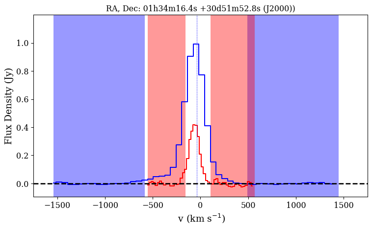
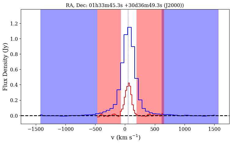
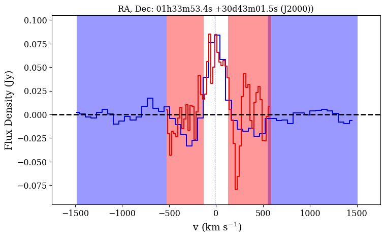
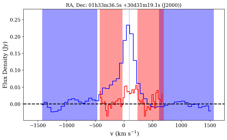
Figure 10: PACS spectra of [C ii] (blue) and [O i](63$\mu$m) (red) at selected positions in M 33. All spectra are shown at their native angular resolution, before convolution to $12^{\prime\prime}$ resolution. The velocities have been corrected for the systemic velocity of M 33 of $-180$ km s^-1. Dashed, vertical lines mark the residual velocity of the H i line (Warner et al. 1973). Spectra are shown after subtraction of polynomial baselines of up to 3rd order. The two red (blue) fields mark the velocity range, which was used to calculate the baseline rms for the [O i] ([C ii]) line. Baselines at more extreme velocities are not shown. [C ii] integrated intensities were calculated over the inner range between the blue fields ($\pm 538$ km s^-1), and the integrated intensities for the [O i] line were calculated over the spectral range (in white) between the red fields. The double-peak structure of the weak [O i] line seen in the right spectrum of the lower row is attributed to baseline noise.

PACS data reduction of the unchopped scans was done using HIPE version 15.0.1 (Ott 2010). The data were calibrated using the PACS calibration tree version 78. The data pipeline was used, including a correction for transients (glitches) and including spectral flat fielding, to obtain level 2 data products for each of the individual 21 ObsIds. Stepping through the pipeline and displaying intermediate results indicated that the “transient correction” is necessary to obtain good final data products. At this point, the “Off” data products were kept separate from the “On” data products. After running this initial pipeline, a script “Spectoscopy: Mosaic multiple observations” from the menu “PACS Useful scripts” was used to combine the individual ObsIds. This script was modified slightly to average all Off-positions together, subtract them from each On-position, and to create the final data cube. The output is a single FITS file that contains the spectra at each spaxel of the combined map on a $3^{\prime\prime}$ grid. Figure 10 shows a few exemplary spectra.

Python scripts were developed to derive line integrated intensities and to estimate the baseline noise. Polynomials of up to third order were fit to the spectra, masking the edges, which suffer from increased noise and artifacts, and also the region around the expected line position from H i data (Warner et al. 1973). The script determined the best fitting polynomial, and subtracted it. Integrated line intensities were derived by summing over a narrow wavelength range, 2.8 times the resolution, centered on the H i velocities at each PACS spaxel.

The baseline noise was estimated by calculating the standard deviation (root mean square, rms) within the wavelength range used to fit the baseline. The spectral noise varies with spaxel. The median baseline noise, that is, the statistical error, are $(1.6\pm 1.1)\cdot 10^{-7}$ erg s^-1 cm^-2 sr^-1  for [C ii], $(3\pm 7)\cdot 10^{-7}$ erg s^-1 cm^-2 sr^-1  for [O i](63$\mu$m). For each position the local 1 $\sigma$ uncertainty was estimated by adding in quadrature the local noise levels and the relative calibration errors of 15% for [C ii] and [O i], respectively.

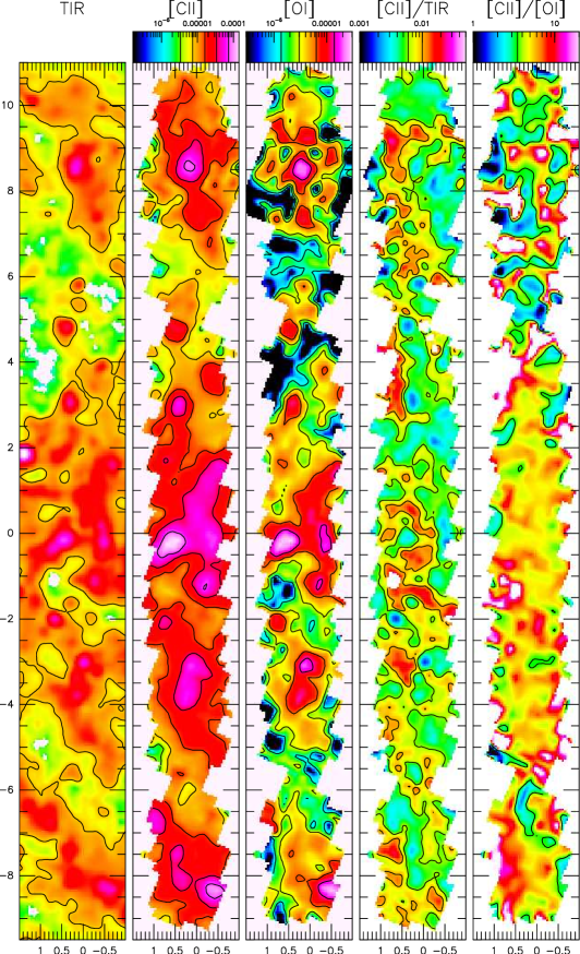
Figure 2: Central part of the PACS maps of M 33. From left to right: intensities of total infrared continuum (TIR), [C ii], [O i](63$\mu$m), [C ii]/TIR, and [C ii]/[O i] intensity ratios. Intensities are in units of erg s^-1 cm^-2 sr^-1. Offsets are in arcminutes relative to the nucleus, after de-rotation of the position angle by 22.5^∘. The TIR contour is at $2\cdot 10^{-3}$ erg s^-1 cm^-2 sr^-1, the threshold intensity used in the correlation plots to distinguish TIR-bright and TIR-weak regions (Figs. 4, 5, 6, 8, 5). The color wedge is the same as in Fig. 1. [C ii] contours are the same as in Fig. 1. [O i] contours are 1.4, 3.0, 6.3, 13.8 in units of $10^{-6}$ erg s^-1 cm^-2 sr^-1. The map of [C ii]/TIR is overlayed with contours at the 0.6% and 1% level of the ratio. The map of [C ii]/[O i] is overlayed with the contour of 3.5. Long tic marks in the color wedges indicate contour levels.

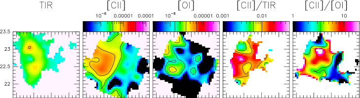
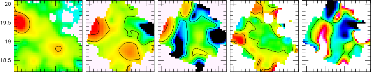
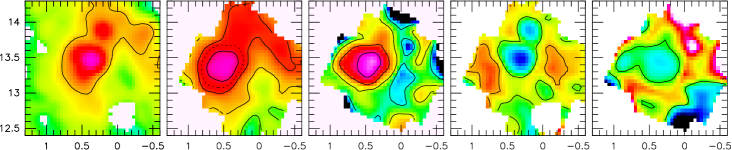
Figure 3: Three northern most regions of M 33 covered with PACS. Top row: Northernmost region. Middle row: Northern region. Bottom row: BCLMP 691. From left to right: intensities of total infrared continuum (TIR), [C ii], [O i](63$\mu$m), [C ii]/TIR, and [C ii]/[O i] intensity ratios. Intensities are in units of erg s^-1 cm^-2 sr^-1. Offsets are in arcminutes relative to the nucleus, the same as in Fig. 2. The TIR color wedge is the same as in Fig. 1. Contours of TIR, [C ii], [O i], [C ii]/TIR, and [C ii]/[O i] are the same as in Fig. 2. The dashed [C ii] contour for BCLMP 691 corresponds to a constant intensity of $22.4\cdot 10^{-6}$ erg s^-1 cm^-2 sr^-1  derived from the best-fitting y-intercept in the correlation plot of $\log$[C ii]/TIR vs. $\log$TIR, for a slope of $-1$ (Fig. 9).

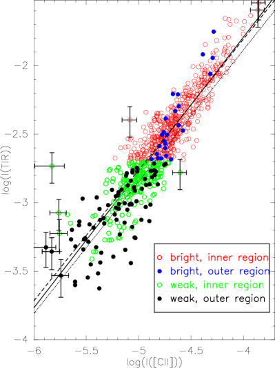
Figure 4: Total infrared continuum intensity (TIR) versus [C ii] intensities in M33. Intensities are given in erg s^-1 cm^-2 sr^-1. Each point corresponds to one position on a $12^{\prime\prime}$ grid at $12^{\prime\prime}$ resolution, with an intensity 3 times above the local rms, for [C ii], [O i], and TIR. Typical $1\sigma$ errorbars are shown. Colors correspond to the four different regions of the inner and outer galaxy, and above and below a TIR threshold, as described in Sec. 3.1. Straight lines delineate the results of unweighted linear least-squares fits to all data (drawn), the inner galaxy (dashed), and the outer galaxy (dotted) (Table 1).

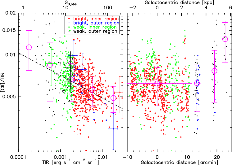
Figure 5: (Left) [C ii]/TIR intensity ratio versus TIR and corresponding FUV field G_0,obs in M 33 (see equation 2 in Sec. 3.1). The large pink points and errorbars show binned ratios (Table 2). Errorbars represent the standard deviation of the data. The dashed line shows the result of an unweighted least-squares fit to $\log$([C ii]/TIR)$=b+m\times\log$TIR and all ratios, which gives $m=-0.16\pm 0.10$ and $b=-2.64\pm 0.26$, with correlation coefficient $r=-0.39$. For a few of the individual points $1\sigma$ errorbars are shown. (Right) [C ii]/TIR versus projected galacto-centric radius in M 33. The large pink points and errorbars show ratios binned over selected ranges of radii (Table 3).

2.2 Total infrared continuum and atomic hydrogen

The integrated intensity of the continuum emission between wavelengths of 1 $\mu$m and 1 mm, the TIR, has been estimated for each pixel from a weighted sum of the MIPS/Spitzer 24 $\mu$m and PACS 70 $\mu$m, 100 $\mu$m, and 160 $\mu$m maps. Before combining these maps, all images were convolved to a common resolution of $12^{\prime\prime}$ using the dedicated kernels provided by Aniano et al. (2011) and regridded to a common reference frame with a pixel size of $3^{\prime\prime}$ projected onto the [C ii] PACS positions. The PACS 70 $\mu$m map (Boquien et al. 2015) was rescaled to MIPS fluxes by multiplying with the MIPS scaling factor ($mc=1.03$) and dividing by the color correction factor ($cc=0.98$) which were interpolated from Table 3 of the PACS report by Müller et al. (2011) assuming a modified blackbody with an emissivity index of $\beta=1.5$ and an average dust temperature of 35 K (Tabatabaei et al. 2014): $S_{70}^{\rm{MIPS}}=mc/cc\cdot S_{70}^{\rm{PACS}}$. Next, the TIR was calculated using weighting factors from Equation 1 and Table 1 of Boquien et al. (2011), and using all data larger than zero:

$$\log S_{\rm{TIR}} = 0.220\cdot\log S_{24}+0.202\cdot\log S_{70}^{\rm{MIPS}}+$$ (1)

$$0.243\cdot\log S_{100}+0.311\cdot\log S_{160}+1.361.$$

In a similar approach, Galametz et al. (2013) used spatially resolved Herschel maps of the KINGFISH sample of nearby galaxies to derive weighting factors to estimate the TIR. Galametz et al. (2013, cf. their Fig. 6) find that the determined calibration coefficients are very similar to those measured in M 33 by Boquien et al. (2011) using Spitzer and Herschel maps.

The median statistical error of the TIR in M 33 as measured in emission free areas, is $(2.0\pm 1.0)\cdot 10^{-5}$ erg s^-1 cm^-2 sr^-1. For each position, the local 1 $\sigma$ uncertainty was estimated by adding in quadrature the statistical error and the relative calibration error of 25%, assuming 20% error on the 160$\,\mu$m data, and $\sim 10$% error on the 100, 70, and 24$\,\mu$m data, respectively (Boquien et al. 2011).

The TIR map (Fig. 1) resulting from Eq. 1, shows the flocculent spiral structure of M 33, a number of prominent giant H ii regions, the arm and interarm regions, together with the drop of intensities with increasing galacto-centric radius.

To estimate the contribution of the cold neutral medium to the [C ii] emission, we used a VLA map of M 33 in the atomic hydrogen 21 cm line at $12^{\prime\prime}$ resolution (Gratier et al. 2010), matching the resolutions of the other data.

3 Analysis

3.1 [C ii] emission and the total infrared continuum

The maps of TIR and [C ii] (Figs. 1, 2, 3) show a striking similarity. Both tracers vary by more than two orders of magnitude in intensity. They are bright in the inner star forming arms and gradually fainter in the outskirts at several kiloparsec radial distance. A correlation plot of TIR against [C ii] shows their tight correlation (Fig. 4). The results of linear least-squares fits to $\log\,I$(TIR) against $\log\,I$([C ii]) are shown in Fig. 4 and Table 1. The scatter is larger at fainter intensities and larger than the statistical errors of the individual positions. To gain more insight, we have subdivided the observed positions between those of TIR intensities above and below a given value, tracing the dense, warm, star-forming spiral arms on the one hand, and the diffuse inter-arm dust on the other hand. A second subdivision distinguishes between the inner and outer galaxy. The TIR threshold and the radial boundary have no specific physical meaning and were selected to emphasize differences between the four regions. We chose a TIR threshold of $2\cdot 10^{-3}$ erg s^-1 cm^-2 sr^-1  (shown as contour in Figs. 2 and 3) and a radial boundary of 2.93 kpc ($12^{\prime}$) to separate the inner and outer galaxy (cf. Verley et al. 2009). The fit slopes and intercepts of the inner and outer regions of the galaxy do not differ within the errors (Table 1). We find indications for a steepening of the slope for the TIR-bright outer regions (Fig. 4).

As the dust grains emitting the observed TIR emission are heated by the stellar radiation field, the TIR can be used to estimate the FUV energy flux G_0,obs, which is given in units of the average radiation field in the solar neighborhood, the Habing field of $1.6\cdot 10^{-3}$ erg cm^-2 s^-1 (Habing 1968):

$$G_{0,\rm{obs}}=C_{1}C_{2}\,\frac{\rm{TIR}}{1.6\cdot 10^{-3}/(4\pi)}$$ (2)

with TIR in units of erg s^-1 cm^-2 sr^-1. The factor of $C_{1}=0.5$ approximately takes into account the absorption of visible photons by grains (Kaufman et al. 1999; Tielens & Hollenbach 1985).

The factor $C_{2}$ corrects for the fraction of FUV photons leaking out of the galaxy. To estimate the FUV attenuation in M 33, Boquien et al. (2015) combined GALEX FUV maps with 24$\mu$m maps, following Kennicutt et al. (2009). The typical attenuation in M 33 is around 0.6 mag in the FUV band, consistent within the scatter with 0.53 mag previously found by Verley et al. (2009). In the low metallicity environment of M 33, about half of the FUV photons are hence on average absorbed by dust and reradiated in the TIR, while the other half escapes, that is, $C_{2}=2$.

In M 33 at 50 pc resolution, the estimated FUV field G_0,obs ranges between $\sim 2$ and 200 (Fig. 5). The selected TIR threshold of $2\cdot 10^{-3}$ erg s^-1 cm^-2 sr^-1  corresponds to a FUV field of G_0,obs$=15$. Further below, we used the observed ([C ii]$+$[O i])/TIR and [C ii]/[O i] ratios together with PDR models of given density and FUV field to improve on this estimate.

The average [C ii]/TIR ratio in M 33 is ($0.64\pm 0.21$)% (Table 2). Figure 5 (Left) shows the data at the individual positions, together with unweighted binned averages. For low TIR values the [C ii]/TIR ratio shows a large scatter with a high averaged value of ($1.1\pm 0.4$)% at $\log$(TIR)=$-3.75$, with the TIR intensities in units of erg s^-1 cm^-2 sr^-1. The binned ratios drop smoothly with TIR, reaching ($0.5\pm 0.1$)% at high TIR values of $\log$(TIR)=$-1.75$. The binned averages are consistent with the results of a linear least-squares fit (Fig. 5).

To explore the [C ii]/TIR variation further, we study its variation with galacto-centric distance (Fig. 5, right). The [C ii]/TIR ratio stays almost constant within a galacto-centric radius of $\sim 4\,$kpc (cf. Verley et al. 2009). The two northern regions show rising [C ii]/TIR ratios, as had already been seen in the ISO/LWS cut (K2013). The northernmost region shows a mean ratio that is a factor 2 higher than in the inner galaxy, $1.3\%$, with an increased scatter of $0.4\%$ (Table 3). The corresponding map (Fig. 3) shows a small region of low [C ii]/TIR ratios, where TIR is just above the threshold of $2\cdot 10^{-3}$ erg s^-1 cm^-2 sr^-1, but surrounded by an extended region of high ratios $>1\%$ where TIR is below the threshold and [C ii] is also weak.

The ISO/LWS cut along the major axis of M 33 (K2013) shows a flat [C ii]/FIR distribution in the inner galaxy, and an abrupt rise of the average ratio in the northern and southern outskirts, at galacto-centric distances beyond $\sim 4.5$ kpc out to $\sim 7.5$ kpc. Using the FIR/TIR correction factors listed for each position in Table A.1 of K2013, the resulting [C ii]/TIR values are consistent within the $1\sigma$ scatter with the ratios determined here. The Herschel/PACS data presented here improve on this work due to their high sensitivities at much better angular resolution, mapping the GMCs also perpendicular to the major axis of M 33.

Table 1: Results of unweighted linear least-squares fits to $\log$TIR=$b+m\times\log$[C ii] (Fig. 4) with TIR and [C ii] in units of  erg s^-1 cm^-2 sr^-1. The Pearson correlation coefficient $r$ serves as a measure of the linear correlation between TIR and [C ii].

Region	$m\pm\sigma$	$b\pm\sigma$	$r$
all	$0.99\pm 0.11$	$2.15\pm 0.52$	0.91
inner	$0.95\pm 0.13$	$2.01\pm 0.60$	0.90
outer	$0.96\pm 0.29$	$1.96\pm 1.50$	0.87

Table 2: Binned [C ii]/TIR ratios shown in Figure 5. The width of the TIR bins is 0.5 dex. Errors of the individual points are ignored.

$\log$ TIR	[C ii]/TIR
	%
all	$0.64\pm 0.23$
$-3.75$	1.13 $\pm$ 0.36
$-3.25$	0.85 $\pm$ 0.39
$-2.75$	0.66 $\pm$ 0.20
$-2.25$	0.56 $\pm$ 0.13
$-1.75$	0.49 $\pm$ 0.10

Table 3: [C ii]/TIR ratios averaged over different galacto-centric distances (cf. Figure 5). Errors of the individual points are ignored.

radial range		[C ii]/TIR
arcsec	kpc	%
$-700..700$	$-2.8..2.8$	$0.62\pm 0.19$
$750..870$	$3.1..3.5$	$0.63\pm 0.23$
$1090..1210$	$4.4..4.9$	$0.77\pm 0.31$
$1320..1410$	$5.4..5.7$	$1.30\pm 0.41$

Table 4: Results of unweighted linear least squares fits to $\log$[O i]$=b+m\times\log$[C ii]. (Fig. 6).

Region	$m\pm\sigma$	$b\pm\sigma$	$r$
bright, inner	$0.84\pm 0.01$	$-1.43\pm 0.86$	0.74
bright, outer	$1.49\pm 0.25$	$1.65\pm 5.65$	0.75

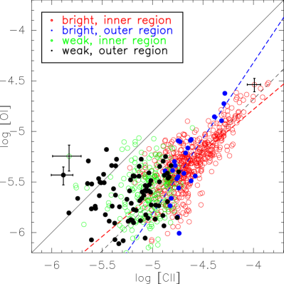
Figure 6: Observed intensities of [O i](63$\mu$m) and [C ii] in M 33 with representative $1\sigma$ errorbars. The straight black line corresponds to a ratio of 1. The dashed black line corresponds to the average [C ii]/[O i] ratio (Table 5). The red and blue dashed lines are the results of unweighted least squares fits to the TIR-bright inner and outer regions, respectively (Table 4).

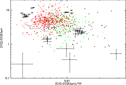
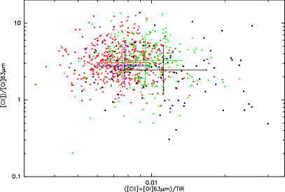
Figure 7: [C ii]/[O i](63$\mu$m) ratio plotted against the ([C ii]+[O i]($63\,\mu$m)/TIR ratio for M 33. [C ii], [O i], and TIR intensities are from positions with intensities above the local $3\sigma$ value. Colors correspond to the four different regions of the inner and outer galaxy, and above and below a TIR threshold, as described in Sec. 3.1. Left: Observed ratios with typical 1$\sigma$ errors. Right: Ratios with corrected [O i] intensities, as described in Sec. 3.2.4. In addition, median and standard deviations are shown for the four regions (errorbars in color) (cf. Table 5).

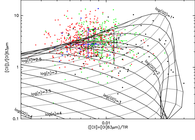
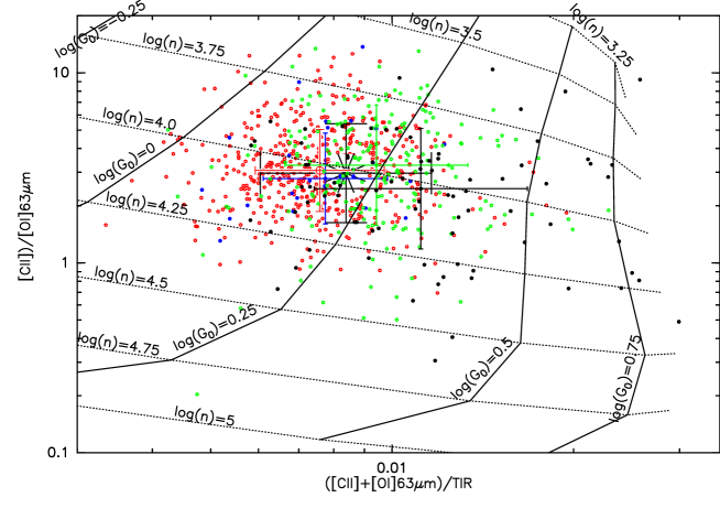
Figure 8: Diagnostic diagram of the [C ii]/[O i](63$\mu$m) ratio plotted against the ([C ii]+[O i]($63\,\mu$m)/TIR ratio for M 33, using the corrected [O i] intensities (see Sec. 3.2.4). Median and standard deviation of the four regions are shown in color, and of all data (star and large errorbars). Colors correspond to the four different regions as described in Sec. 3.1: the TIR bright, inner region (red), the bright, outer region (blue), the weak, inner region (green), and the weak, outer region (black). Superimposed is a grid of constant hydrogen nuclei density $n$ (dashed contours) and FUV field strength $G_{0}$ (solid contours) from PDR models (Kaufman et al. 1999, 2006). We note that for many ratios there are two solutions for $n$, $G_{0}$. Upper panel: Solutions with moderate $n$, $G_{0}$. Lower panel: Low-FUV solutions.

Table 5: Median [C ii]/[O i] and ([C ii]+[O i])/TIR ratios and rms values as observed and after correction for [O i] self absorption. Solutions of the PDR models of Pound & Wolfire (2008); Kaufman et al. (2006) are shown for the median ratio of all positions and for position #1 with one of the highest observed [C ii] intensities $1.2\cdot 10^{-4}$ erg s^-1 cm^-2 sr^-1.

Region	[C ii]/[O i]	([C ii]+[O i])/TIR	Solutions of PDR models
			Moderate solution		low-FUV solution
			$n$	$G_{0}$	$n$	$G_{0}$
		%	[cm-3]		[cm-3]
	Observed ratios
all	$4.51\pm 2.58$	$0.75\pm 0.31$	60	20	$10^{4}$	1
bright, inner	$4.79\pm 2.43$	$0.68\pm 0.19$	60	20	$10^{4}$	1
bright, outer	$3.71\pm 3.68$	$0.72\pm 0.19$	30	20	$10^{4}$	1
weak, inner	$3.83\pm 2.54$	$0.91\pm 0.27$	100	30	$10^{4}$	1
weak, outer	$3.01\pm 2.36$	$1.07\pm 0.54$	300	60	$10^{4}$	1
	Ratios with corrected [O i]
all	$3.0\pm 2.1$	$0.82\pm 0.53$	$200$	60	$10^{4}$	1.5
bright, inner	$3.06\pm 1.92$	$0.76\pm 0.2$	$200$	60	$10^{4}$	1.5
bright, outer	$2.78\pm 2.69$	$0.77\pm 0.18$	$200$	70	$10^{4}$	1.5
weak, inner	$3.27\pm 2.28$	$0.94\pm 0.89$	$300$	60	$10^{4}$	1.5
weak, outer	$2.46\pm 2.02$	$1.12\pm 0.55$	$600$	80	$10^{4}$	2.0
#1	$4.59\pm 0.97$	$0.76\pm 0.25$	$900$	$20$	$5\cdot 10^{3}$	3.0

3.2 Emission of [C ii], [O i] 63$\mu$m, and the TIR

The critical densities of the [C ii](158$\mu$m) and [O i](63$\mu$m) lines for excitation by collisions with H are $3\cdot 10^{3}$ cm^-3 and $5\cdot 10^{5}$ cm^-3, respectively, with upper energy levels $E/$k_B of 92 K and 228 K, respectively (Kaufman et al. 1999). In contrast to the [C ii] line, the [O i](63$\mu$m) line is expected to be excited almost exlusively in the dense, warm interface regions of UV illuminated molecular clouds. The distribution of these two emission lines reflects these strong differences in excitation requirements. The intensities of [C ii] and [O i] emission are well correlated near the peaks and ridges of the spiral arms of M 33, as is seen in the maps of the central region and of BCLMP 691 (Figs. 2, 3) and in the correlation plot (Fig. 6, cf. Table 4). At lower intensity levels of [C ii] and [O i], in the more diffuse inter-arm regions, the correlation between the two gas tracers is weak. This is seen most prominently in the maps of the two northern most regions (Fig. 3).

As expected, [C ii] is stronger than [O i] at most positions. The observed [C ii]/[O i]($63\mu$m) ratio ranges between $\sim 0.3$ and 20 with a median of $4.5\pm 2.6$. The observed ([C ii]+[O i]($63\,\mu$m)/TIR ratios vary between 0.3 and 2.9% with a median of $0.8\pm 0.3$% (Fig. 7). Table 5 lists the average values and the scatter for the four regions defined in Section 3.1. The TIR bright positions all show ratios of [C ii]/[O i]$>1$ and ([C ii]+[O i])/TIR$<$2%, while the positions where [O i] intensities exceed those of [C ii], and ([C ii]+[O i])/TIR$>2$% all lie in the TIR weak regions.

PDR models may allow one to estimate the local excitation conditions, the local densities and the local FUV fields. In order to compare the observations with the predictions of PDR models, we need to consider other components of the ISM that may contribute to the emission. A part of the [C ii] emission may stem from the cold neutral medium (CNM) or from a diffuse ionized medium. The [O i](63$\,\mu$m) line may become optically thick and be affected by foreground absorption. Below, we discuss these possibilities.

Table 6: Assumptions to estimate the fraction of [C ii] emission from the cold neutral medium (CNM). $N$(H i,PDR) is the estimated column density of atomic hydrogen at the surfaces of the PDRs. $X$(C⁺) is the fractional abundance of C⁺, $n_{\rm CNM}$ and $T_{\rm CNM}$ are density and temperature of the CNM.

$N$(H i,PDR)	$3.25\cdot 10^{20}$ cm-2
$X$(C+)	$5.9\cdot 10^{-5}$
$n_{\rm CNM}$	100 cm-3
$T_{\rm CNM}$	80 K

3.2.1 [C ii] from the cold neutral medium

To estimate the contribution of the cold neutral medium (CNM) to the observed [C ii] emission, we used H i VLA data, at all positions at which [C ii] has been detected, and at almost the same angular resolution. Following the approach of K2013, we first corrected the H i line intensities for the contribution from the surfaces of PDRs assuming a typical $G_{0}/n$ ratio of 10^-3. Next, the [C ii] emission from the remaining neutral gas, the CNM, was estimated assuming a given fractional abundance of C⁺/H in the low-metallicity environment of M 33, optically thin H i and [C ii] emission, and a density and temperature which are typical for diffuse atomic clouds (Table 6). While some regions at larger galacto-centric distances show enhanced CNM fractions, as already seen by K2013, the average CNM contribution is only $\sim 10$% (Fig. 11), less than the estimated [C ii] calibration error. We do not subtract this small contribution from the CNM from the observed [C ii] intensities to estimate the [C ii] emission from PDRs.

3.2.2 [C ii] from the ionized medium

Another part of the [C ii] emission may not arise from the neutral gas of PDRs modeled by Kaufman et al. (2006), but from the diffuse, ionized gas. Observations of the [N ii](122$\mu$m, 205$\mu$m) lines would allow us to determine electron densities and the importance of the ionized gas (Oberst et al. 2006; Croxall et al. 2012, 2017). Parkin et al. (2013a, 2014) studied maps of [C ii], [O i], and TIR emission in M 51 and Centaurus A. PDR models better fit the observed [C ii]/[O i] and [C ii]$+$[O i]/TIR ratios after correcting for the fraction of [C ii] emission originating from the ionized medium using [N ii](122$\mu$m, 205$\mu$m). They estimate that 70-80% of [C ii] arise in ionized gas of the nucleus and center of M 51, 50% in its arm and interarm regions. In Centaurus A the ionized fraction is 10-20%. Hughes et al. (2015) use the [N ii](205 $\mu$m) line to estimate fractions of $\sim 16-64\%$ in NGC 891. They also explore the use of an empirical relation between [N ii] and 24 $\mu$m emission, to construct a more complete map of the [C ii] fraction from the ionized gas. For M 33, we do not attempt to correct the [C ii] intensities for the contribution from the ionized gas as observations of the [N ii] lines are missing.

3.2.3 TIR

A fraction of the TIR emission may stem from non-PDR phases of the ISM like the CNM. We did not try to correct the TIR emission for these contributions before using the PDR models. However, the correlation between TIR and H i intensities is poor in M 33 (Fig. 12). An unweighted linear least-squares fit gives a correlation coefficient of $r=0.45$, which is much lower than for the TIR-[C ii] relation. This indicates that most of the TIR emission stems from PDR regions, as the CNM contribution to the [C ii] emission is also low.

3.2.4 Self-absorbed [O i] (63$\,\mu$m) emission

The [O i](63$\mu$m) line is expected to have a higher opacity than the [C ii] line and hence may be affected by self-absorption caused by cold foreground clouds of atomic oxygen, as has been seen in velocity resolved spectra and with narrow beams toward bright background sources in the Milky Way (Schneider et al. 2018; Gerin et al. 2015; Leurini et al. 2015; Karska et al. 2014; Lis et al. 2001; Timmermann et al. 1996). Spectra of the [O i](63$\mu$m) line taken toward ULIRGs are often heavily self-absorbed (Rosenberg et al. 2015). Israel et al. (2017) also used PACS/Herschel to observe the center of Centaurus~A. Using PDR models allowed them to compare the observed [O i](63 $\mu$m) intensity with the intensity predicted from modeling the emission of other FIR lines. In the circumnuclear disk Israel et al. (2017) find high optical depths of the [O i] line of $1.0-1.5$. While these PDR models take into account optical depth effects of the spectral lines emerging from the simulated slab of gas, they do not consider possible absorption by foreground gas of different excitation conditions.

The intrinsic line widths observed in M 33 in [C ii], CO and H i are far smaller than the velocity resolution of PACS/Herschel ($\sim 90$ km s^-1). Using HIFI/Herschel HerM33es observations, Mookerjea et al. (2016) and Braine et al. (2012) find full-widths at half-maximum (FWHM) of [C ii] of 7 to 17 km s^-1 in three regions along the major axis of M 33: BCLMP 302, BCLMP 691, and the nucleus. Druard et al. (2014) and Gratier et al. (2017) studied the variation of FWHMs derived from maps of the complete galaxy in CO 2–1 taken with the IRAM 30m telescope and H i taken with the VLA. The line widths averaged in radial bins of 1 kpc drop with distance, out to 7.5 kpc: from about 8 to 5 km s^-1 for CO, and from about 17 to 12 km s^-1 for H i. As the [O i](63$\mu$m) line is expected to arise from the dense, warm cloud interfaces, its linewidths should be similar to those of CO, and smaller than those of [C ii], which may also trace other, more diffuse phases.

Assuming low densities in the cold, foreground layers of gas, the majority of the oxygen atoms are in their ground state, allowing to derive an upper limit of the [O i] opacities. The column density of atomic oxygen can then be approximated in terms of the opacity $\tau_{0}$ at the center velocity of the $J=1-2$ [O i] 63$\,\mu$m line by

$$N(\rm{OI})=2\cdot 10^{17}\,\tau_{0}\,\Delta v_{\rm{FWHM}}$$ (3)

in cm^-2, with the FWHM line width in km s^-1 (Vastel et al. 2002; Liseau et al. 2006). For a typical line width of 7 km s^-1 (see above) and an average oxygen abundance of $4\cdot 10^{-4}$ in M 33 (see below), the line center opacity exceeds 1 for $N($[O i]$)=1.4\cdot 10^{18}$ cm^-2 and $N$(H)$>3\cdot 10^{21}$ cm^-2. Following Crawford et al. (1985), the opacity is more generally written as function of local density $n$ and temperature $T$ of the [O i] two level system:

$$\tau_{0}= \frac{\lambda^{3}\,A_{\rm{ul}}}{8\pi\Delta v_{\rm{FWHM}}}\Bigl{[}(1+\frac{n_{\rm{cr}}}{n})\exp(228/T)-1\Bigr{]}$$ (4)

$$\Bigl{[}\frac{\frac{3}{5}\exp(-228/T)}{1+\frac{3}{5}\exp(-228/T)+\frac{n_{\rm{cr}}}{n}}\Bigr{]}\,\,N(\rm{OI})$$

with the Einstein A-coefficient $A_{\rm{ul}}=8.46\cdot 10^{-5}$ s^-1, the critical density $n_{\rm{cr}}=4.7\cdot 10^{5}$ cm^-3 for collisions with H-atoms, $h\nu/k_{B}=228$ K, and the ratio of statistical weights $g_{u}/g_{l}=3/5$. The resulting hydrogen column density for a line center opacity of the [O i] 63$\mu$m line of 1 agrees within 10% with the result from Eq. 3 for $10^{3}$cm^-3 $\leq$ n $\leq$ $10^{5}$cm^-3 and 20 K $\leq$ 400 K. This is also consistent with the results of RADEX radiative transfer modeling (van der Tak et al. 2007).

We used the dust emission to estimate total hydrogen column densities at the positions observed in M 33 by fitting a single modified black body (MBB) to the 70, 100, 160$\,\mu$m fluxes, while keeping $\beta=1.5$ constant, deriving the dust temperature and dust mass surface density. To find the best-fitting SED for each pixel on the map, a $\chi^{2}$ function was minimized using the Levenberg-Marquardt algorithm (Xilouris et al. 2012). For a constant gas-to-dust ratio of 150 (Kramer et al. 2010), this implies typical hydrogen column densities of $2.4\cdot 10^{21}$ cm^-2 per beam, implying moderate [O i] opacities of 0.7. Hydrogen column densities peak at $\sim 10^{22}$ cm^-2 ($A_{V}\sim 10$ mag) (Fig. 13), with corresponding [O i] optical depths of $\sim 3$.

The standard PDR models of Kaufman et al. (2006); Pound & Wolfire (2008), used below, assume homogeneous slabs of an optical extinction of $A_{V}=10$ mag. The models compute a simultaneous solution for the chemistry, the thermal balance, and also the radiative transfer. As already said above, optical depths effects of the emergent line emission are taken into account. From these models, it is known that the [O i](63$\mu$m) line emission becomes optically thick, with opacities of several, over the entire parameter space of $n$, $G_{0}$ sampled by the models. These models do, however, not consider absorption of the emission of warm background gas by colder foreground gas, as would be expected for GMCs which are internally heated by star-formation.

To estimate the possible effect of foreground absorption, we modeled the reduction in line center brightness temperatures assuming for each of the two source components beam filling factors of 1 and

$$T_{\rm R}=J_{\nu}(T_{\rm{ex}})\,[1-\exp[-\tau_{0}]]$$ (5)

with $J_{\nu}(T_{\rm ex})=228\,(\exp(\frac{228}{T_{\rm ex}})-1)^{-1}$. The two source components are added, allowing for foreground absorption:

$$T_{\rm R}=T_{\rm{R,fg}}+\exp(-\tau_{\rm{0,fg}})\,\,T_{\rm{R,bg}}.$$ (6)

Using in addition Eq. 4 for the opacity of the [O i] line, we furthermore assumed for both components FWHM linewidths of 7 km s^-1 and a density of $n=10^{4}$ cm^-3. We assume that the background GMCs lie on average in the mid-plane of the galaxy and considered only half of the total column density in the following. In the absence of high-resolution spectra, which would allow for fitting free parameters to the observed line profiles (e.g., Graf et al. 1993), we assumed here ad-hoc that 80% of this half total column density is in the foreground components at 15 K, while 20% is in a background component at $200$ K. This results in a reduction of the emerging line intensity by a factor of 3.3 for the highest total column densities of $10^{22}$ cm^-2 observed. The median corrections are $1.32\pm 1.8$. The median corresponds to a total column density of $\sim 1.17\cdot 10^{21}$ cm^-2. A smaller fraction of foreground gas would lead to lower reduction factors and vice versa. We take these estimates as rough, first estimates and apply them to the data before comparing them with PDR models.

Figure 7 shows the observed intensity ratios and the ratios after correction of the [O i] intensities. After the correction, the [C ii]/[O i](63$\,\mu$m) ratio of all positions ranges between 0.13 and 13.7 with a median of $3.0\pm 2.1$, and the ([C ii]$+$[O i](63$\,\mu$m))/TIR ratio ranges between 0.3 and 11.6% with a median of $0.8\pm 0.5$%. The median ratios do not differ much between the different regions in M 33 (Table 5).

3.2.5 PDR models

To better understand the observed ratios of [C ii]/[O i] and ([C ii]+[O i])/TIR, corrected for [O i] self-absorption, we compare them with the predictions of PDR models (Kaufman et al. 2006; Pound & Wolfire 2008). These assume FUV illuminated slabs of an optical exinction of $A_{V}=10$ mag and solar metallicities, for a range of local densities and FUV fields. The FUV field $G_{0}$ used in the PDR models is the local FUV field heating the slabs of dust and gas, leading to emission of the TIR, [C ii], and [O i]. The ratio of the local $G_{0}$ from the models and the G_0,obs from the observed TIR emission gives the beam filling factor of the emitting clouds. Beam filling factors in the observed ratios cancel out under the reasonable first order assumption that the three tracers ([C ii], [O i], TIR) have the same filling factor. We ignore here that the excitation conditions for the [O i] line indicate a somewhat smaller beam filling factor than for the other two tracers.

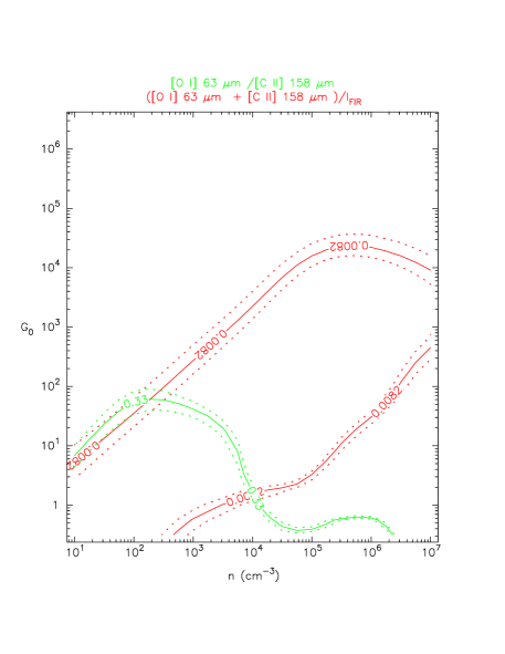
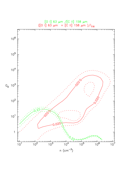
Figure 15: Contours of the ratios of [O i]/[C ii], and ([C ii]+[O i])/TIR, with [O i] corrected (Table 5), as a function of cloud density $n$ and incident FUV flux $G_{0}$ using the PDR model of Kaufman et al. (2006). Left: Median ratios of all positions. Right: Ratios at a [C ii] peak position.

For many of the observed ratios, the PDR models do not provide a unique $G_{0},n$ solution. For these positions, two solutions exist, one at high density and low FUV field, and another one at moderate values of $G_{0}$ and $n$. An example is shown in Figure 15, which exhibits contours of the average ratios of all observed positions (Table 5) as a function of density and FUV field of the Kaufman PDR models. There exist two best-fitting solutions, which are both consistent with the ratios of [C ii], [O i], and TIR.

Solutions with moderate $n$, $G_{0}$ exist for the bulk of the ratios in M 33, after correcting for [O i] self-absorption (Fig. 8 Upper panel). The ratios span the range of $\log(G_{0})<3$ and $1\la\log(n/$cm^-3$)\la 4.25$. The average ratios of all four regions can be explained by FUV-fields of $n\sim 2\cdot 10^{2}$ cm^-3 and $G_{0}\sim 60$ (Fig. 15, Table 5). The observed FUV fields G_0,obs range between 2 and 200, which indicates beam filling factors of about 1. The average ratios of the four regions do not differ much and lead to similar best fitting $n$, $G_{0}$ solutions. Even after correcting the [O i] intensities, some of the ratios still lie outside of the parameter space spanned by the moderate solutions: for example the ratios with ([C ii]+[O i])/TIR $\sim 0.8\%$ and [C ii]/[O i]$>4$. Corrections of the [C ii] intensities for contributions from the diffuse, ionized gas may, however, move all points to lower [C ii]/[O i] ratios and lower ([C ii]+[O i])/TIR rations, and into this parameter space.

The low-FUV solutions of the PDR models do, on the other hand, cover the entire range of ratios (Fig. 8 Lower panel). The ratios lie in the regime $0\la\log\,G_{0}\la 0.75$ and $3.5\la\log(n/$cm^-3$)\la 4.5$. The average of all ratios is best fit by $n\sim 10^{4}$ cm^-3, $G_{0}\sim 1.5$ (Fig.15, Table 5). Given the range of observed G_0,obs, this would indicate beam filling factors $\Phi_{\rm{G0}}$ of between $\sim 1$ for the regions with the lowest TIR and $\sim 100$ for the active arm regions with the highest observed TIR. While a fraction of the PDRs along the lines-of-sight may be represented by the low-FUV solution, this cannot be the sole solution. Such a high number of PDRs along the lines-of-sight seems not consistent with the observed peak optical extinctions of $A_{V}\sim 10$ mag, which resemble those of a single PDR model slab. However, only the surface columns of these models of about 1 mag, or of a hydrogen column density of $\sim 10^{21}$ cm^-2, emit [C ii] (cf. Fig. 2 in Kaufman et al. (1999)) and much of the remaining, deeper layers may not exist. High filling factors also seem not consistent with the relatively short lines-of-sight in M 33 with its moderate inclination of only $56\degr$. Comparing the observed [C ii] intensities with those predicted by the PDR models also gives high beam filling factors for the low-FUV solutions. Table 5 lists the ratios for a position with particularly strong [C ii] intensity. The best fitting low-FUV solution for this position is $n=5\cdot 10^{3}$ cm^-3, $G_{0}=3$ (Fig.15). For this solution, the ratio of observed to modeled [C ii] intensity is $\Phi_{\rm{CII}}\sim 10$, which again seems difficult to reconcile with the models. For the moderate solution at the [C ii] peak position, on the other hand, $\Phi_{\rm CII}$ is $\sim 1$.

The degeneracy of the PDR model solutions has been discussed, for example by Hughes et al. (2015); Parkin et al. (2013b); Kramer et al. (2005); Higdon et al. (2003), and Malhotra et al. (2001) for a variety of normal galaxies, who all prefer the moderate solution, often argueing that the low-FUV solution would require far too many PDR slabs along the lines-of-sight to be consistent with the observed intensities.

However, it is also clear that GMCs and their OB associations illuminating gas and dust show structure on a wide range of scales, and that the PDR model slab of constant volume and column density, illuminated by a constant FUV field is only a first order approximation. The inner parts of the GMCs and their OB associations and H ii regions are illuminated by high FUV-fields, while the less dense, colder, outer, and more remote, diffuse parts of the GMCs are illuminated by much lower FUV-fields. We therefore cannot exclude that both solutions of the PDR models are at play along the lines-of-sight in M 33.

Detailed modeling of the spectral energy distributions (SEDs) may shed light on the relative fractions of gas and dust which exhibit the two solutions of the Kaufman PDR models. Aniano et al. (2012) define PDRs as those reagions which are heated by starlight intensities which are a factor 100 or more higher than the ISRF in the solar neighborhood (Mathis et al. 1983), $U>100$, tracing massive star forming regions heated by OB stars. They use Draine & Li (2007) dust models, which assume a distribution of radiation fields between a minimum and a maximum value, fitting them to the observed SEDs between 3.6 $\mu$m and 500 $\mu$m at each position of the galaxies NGC 628 and NGC 6946, creating maps of the PDR fraction. They find that only a fraction of 12% to 14% of the TIR emission stems from such PDRs. More than 85% of the TIR emission in these two galaxies stems from the diffuse ISM heated by low starlight intensities. The latter regions may resemble the regions in M 33 which are characterized by the low-FUV solution of the Kaufman PDR models.

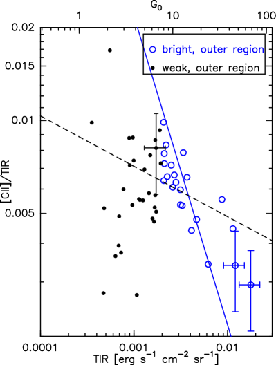
Figure 9: [C ii]/TIR intensity ratio versus TIR for the northern H ii region BCLMP 691 in M 33. The blue drawn line shows the result of an unweighted linear least-squares fit to the TIR-bright data of BCLMP 691 varying only the y-intercept, while keeping the slope fixed at $-1$. The black dashed line shows the result of an unweighted linear least-squares fit to all M 33 data (cf. Fig. 5). A few typical 1$\sigma$ errorbars are shown.

3.3 Metallicities

To first order, one may expect that low metallicities lead to a rise of [C ii]/TIR ratios, as a lowered dust abundance leads to deeper penetration lengths of UV photons, increasing the [C ii] surface layers (Bolatto et al. 1999). This may increase [C ii] intensities, while the thermal dust flux stays about constant (Israel et al. 1996). Indeed, low metallicities have been proposed to explain the observed high [C ii]/TIR ratios found for example in dwarf galaxies (Cormier et al. 2015) and in the outskirts of spirals (e.g., Kapala et al. 2015, 2017).

M 33 exhibits about half solar metallicities together with shallow gradients of dropping metallicities with increasing galacto-centric radius (Magrini et al. 2010). Toribio San Cipriano et al. (2016) measured radial abundance gradients of O/H and C/H from observations of H ii regions in M 33. From optical recombination lines they find:

$$12+\log({\rm O/H}) = 8.76-(0.33\pm 0.13)\times R/R_{25}$$ (7)

$$12+\log({\rm C/H}) = 8.64-(0.61\pm 0.11)\times R/R_{25}.$$ (8)

The value of the 25th mag B-band isophotal radius ($R_{25}$) is $28$ arcmin (6.84 kpc). This is the first work to discuss the C/H abundance gradient of M 33 based on more than just two H ii regions (cf. the discussion in Toribio San Cipriano et al. 2016). The observed C/H gradient is about twice as steep as the O/H gradient, similar to what is found in other small galaxies with subsolar metallicities. The observed metallicity gradient may contribute to the observed indications of a rise of the [C ii]/TIR ratio in the outer regions of M 33 (Fig. 5). However, the scatter of the observed [C ii]/TIR ratio at a given radial distance in M 33 (Fig. 5) and hence about constant metallicity, indicates that other mechanisms can become important.

Here, we take as one example the H ii region BCLMP 691, which is located at a galacto-centric distance of 3.3 kpc in the far north of M 33 (Braine et al. 2012) at about constant metallicity (Eq. 8). For a small region of $\sim 0.9$ arcmin² above the TIR threshold, BCLMP 691 exhibits a marked drop of the observed [C ii]/TIR ratio from the outskirts of the H ii region to its center and the peak of TIR emission by more than a factor of 3, from $\sim 1$% to $0.3$% (Figs. 3, 9).

For optically thin emission, the TIR equals

$${\rm TIR}=\int B_{\nu}(T_{d})\tau_{d}d\nu=\Sigma_{d}\kappa_{0}\int B_{\nu}(T_{d})(\nu/\nu_{0})^{\beta}d\nu$$ (9)

with the total dust mass surface density $\Sigma_{d}$, the line-of-sight (l.o.s.) weighted averaged dust temperature $T_{d}$, the Planck function $B_{\nu}$, the opacity $\tau_{d}$, the average grain cross-section per gram $\kappa_{0}$ at frequency $\nu_{0}$, and the l.o.s. averaged dust emissivity index $\beta$, assuming optically thin emission.

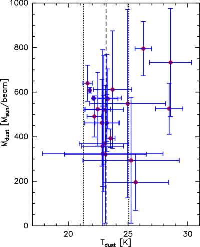
Figure 14: Dust mass surface density vs. dust temperature, derived from fits of modified black bodies, for the TIR bright positions in the H ii region BCLMP 691. The thick dashed line shows the median dust temperature and thin dashed lines correspond to the rms scatter.

Figure 9 shows the observed $\log$[C ii]/TIR vs. $\log$TIR in BCLMP 691. A linear least squares-fit to the positions above the TIR threshold (Fig. 3), keeping the slope fixed to $-1$ results in a correlation coefficient of $r=-0.84$, indicating a good correlation. This slope is consistent with a constant slab of [C ii] emission of $2.2\cdot 10^{-5}$ erg s^-1 cm^-2 sr^-1, the dashed contour in the corresponding [C ii] map (Fig. 3). The [C ii] map indeed exhibits a roughly constant emission over the TIR-bright region, indicating a constant column density and excitation temperature. MBB fits to the SEDs within the small area around the peak of TIR emission in BCLMP 691, where TIR intensities are above the threshold, show that dust temperatures stay fairly constant ($23.2\pm 1.9$ K) with a median value of the estimated errors of $T_{\rm{dust}}$ of 1.3 K. On the other hand, the dust mass surface densities vary by a factor of $\sim 4$ between 200 and 800 $\mathrm{M}_{\odot}$/beam (Fig. 14), a variation which is a factor 3.5 larger than the median of the estimated errors, which is 170 $\mathrm{M}_{\odot}$/beam. The observed steep drop of [C ii]/TIR with TIR in a region of about constant metallicity is hence naturally explained.

4 Summary and conclusions

The emission lines of [C ii] and [O i](63$\mu$m) were mapped along the major axis of the Local Group galaxy M 33. These maps have a width of $\sim 370$ pc and cover a region of 38 arcmin² at 50 pc resolution, allowing to resolve arm and interarm regions. The southern most region lies at 2 kpc galacto-centric distance and, located at the other side of the galaxy, the northern most region lies at 5.7 kpc distance. These maps much improve on the 1-dimensional [C ii] cut at 280 pc resolution, which had been observed along the major axis of M 33 using ISO/LWS (Kramer et al. 2013, K2013).

We combined full-galaxy maps at 24$\mu$m, 70$\mu$m, 100$\mu$m, and 160$\mu$m to construct a map of the total infrared continuum emission (TIR), integrated between 1$\mu$m and 1000$\mu$m wavelength using the kernels provided by Aniano et al. (2011) and the weighting factors derived by Boquien et al. (2011). The observed range of TIR intensities translates to a range of FUV fluxes of G_0,obs$\sim 2$ to 200 in units of the average Galactic radiation field.

We find that the TIR and [C ii] intensities are tightly correlated over two orders of magnitude. The average [C ii]/TIR ratio of $0.64\pm 0.23$% is not significantly higher than the average [C ii]/TIR ratio of $0.48\pm 0.21$% found in a sample of 54 nearby galaxies by Smith et al. (2017). [C ii]/TIR ratios observed in the two northern most regions at 4.5 and 5.5 galacto-centric distances show increasing average ratios of 0.8 and 1.3, respectively. The large-scale variation of the [C ii]/TIR ratios is consistent with the ISO/LWS observations. The resolution and extent of the PACS map allows to distinguish between the diffuse inter-arm regions of the inner and outer galaxy, and the arm regions. The [C ii]/TIR ratio averaged over bins of 0.5 dex decreases with increasing TIR from $1.1\pm 0.4$% for regions with weak TIR emission to $0.5\pm 0.1$% for the arm-regions with highest TIR, while the scatter of binned averages of the [C ii]/TIR ratios decreases as well.

The drop of [C ii]/TIR ratios toward sites of massive star forming regions, where TIR peaks, is most clearly visible in the [C ii]/TIR map of one of the northern H ii regions, BCLMP 691, at 3.3 kpc galacto-centric distance, for positions where TIR is bright. In this case, the drop of [C ii]/TIR ratios is consistent with a [C ii] surface layer of constant intensity, which is independent of TIR. The rise of TIR is caused by a rise of dust mass surface densities, for about constant dust temperatures and emissivities, as is confirmed by the results of modified black body (MBB) fits. For this H ii region, the observed steep drop of [C ii]/TIR with TIR in a region of about constant metallicity is hence naturally explained. However, this does not rule out that on larger scales the drop of metallicities with galacto-centric distance observed in M 33 (Magrini et al. 2010) is decisive to explain the observed drop of [C ii]/TIR with TIR on these scales.

In M 33, [C ii] intensities are stronger than those of the [O i](63$\mu$m) line at almost all positions. The [C ii]/[O i] ratio varies between $\sim 0.2$ and 20, with a mean of $4.5\pm 2.6$. At first glance, the [O i] and [C ii] maps of the inner galaxy resemble each other. However, closer inspection shows that [O i] and [C ii] are only correlated in the TIR-brightest regions while there is only little correlation of both tracers in the TIR weak regions. The observed ([C ii]$+$[O i])/TIR ratio varies between $\sim 0.3\%$ and 3%, with an average of $0.75\pm 0.3$%.

Data of atomic hydrogen, taken with the VLA at the same resolution as the [C ii] data, were used to estimate the contribution of the cold neutral medium (CNM) to the observed [C ii] emission, following the approach of K2013. As anticipated from this work, the averaged contribution is only $\sim 10$%. We did not correct the [C ii] emission for this minor contribution. Modified black bodies were fit to the continuum emission at 70, 100, 160 $\mu$m to derive dust temperatures and surface densities, which were used to estimate total gas and O column densities, and the optical depths of the [O i](63$\,\mu$m) line. A simple model of cold foreground and warm background gas then allowed us to estimate that for the highest H i colunn densities of $10^{22}$ cm^-2, [O i](63$\,\mu$m) line intensities are reduced by a factor of 3.3, while the median correction factor is $1.3\pm 1.8$. The [O i] data were corrected for this effect. An additional correction of the [C ii] data, for diffuse, ionized gas, was not attempted here.

The observed [C ii]/[O i] and ([C ii]+[O i])/TIR ratios were corrected for [O i] foreground absorption, and then compared with standard PDR models (Kaufman et al. 2006). Averages of all observed ratios are similar to the averages of the four individual regions. They all show two solutions of the PDR models, a moderate solution with $n\sim 2\cdot 10^{2}$ cm^-3, $G_{0}\sim 60$, and a low-FUV solution with $n\sim 10^{4}$ cm^-3, $G_{0}\sim 1.5$. The bulk of the observed positions can be modeled by a moderate solution. This solution implies low beam filling factors of $\sim 1$. The low-FUV solution, on the other hand, cannot be the sole solution for all gas along the lines of sight, as it would imply very high beam filling factors $\gg 1$, which are inconsistent with the observed FUV fields, the [C ii] intensities, and the total column densities.

Appendix A Observing parameters of PACS spectroscopy observations

Table 7: Observing parameters of all 22 fields mapped in M 33 with Herschel/PACS in line spectroscopy mode.

Target-Name	RA	Dec.	Integr. Time	ObsID	Obs. Day
	(eq2000)		(sec)
M33-1350N	1h34m31.15s	+31d00m23.90s	6777	1342213044	616
M33-1150N	1h34m25.19s	+30d57m19.20s	6779	1342213043	616
M33-800N	1h34m14.80s	+30d51m55.80s	6781	1342213045	616
M33-600N	1h34m08.80s	+30d48m51.00s	6779	1342213046	616
M33-500N	1h34m06.12s	+30d47m19.26s	3876	1342189072	238
M33-400N	1h34m02.90s	+30d45m46.20s	6777	1342212583	609
M33-350N	1h34m01.42s	+30d45m00.10s	6777	1342212582	609
M33-250N	1h33m58.45s	+30d43m27.70s	6777	1342212579	609
M33-200N	1h33m57.00s	+30d42m41.50s	6777	1342212540	608
M33-150N	1h33m55.48s	+30d41m55.30s	6775	1342212538	608
M33-100N	1h33m54.00s	+30d41m09.10s	6775	1342212536	608
M33-50N	1h33m52.51s	+30d40m22.90s	6775	1342212534	608
M33	1h33m51.02s	+30d39m36.70s	6775	1342213047	616
M33-50S	1h33m49.54s	+30d38m50.60s	6775	1342212535	608
M33-100S	1h33m48.10s	+30d38m04.30s	6775	1342212537	608
M33-150S	1h33m46.58s	+30d37m18.20s	6773	1342212539	608
M33-200S	1h33m45.10s	+30d36m31.90s	6773	1342212578	609
M33-250S	1h33m43.61s	+30d35m45.80s	6773	1342212580	609
M33-300S	1h33m42.10s	+30d34m59.50s	6773	1342212581	609
M33-400S	1h33m39.20s	+30d33m27.20s	6773	1342212584	609
M33-450S	1h33m37.68s	+30d32m41.00s	6773	1342212585	609
M33-500S	1h33m36.20s	+30d31m54.80s	6773	1342212586	609

Appendix B Figures

Figure 11: Fraction of [C ii] emission from the cold neutral medium (CNM), estimated from H i emission.

Figure 12: TIR versus H i intensities in M 33. Intensities are given in erg s^-1 cm^-2 sr^-1. Typical $1\sigma$ errorbars are shown. For H i we assume an calibration error of 15% (cf. K2013). The drawn line shows the result of an unweighted linear least-squares fit to $\log\,{\rm TIR}=b+m\times\log\,{\rm HI}$, which gives a slope $m=0.48\pm 0.11$, y-intercept $b=3.07\pm 1.32$, and correlation coefficient $r=0.45$.

Figure 13: Total hydrogen column densities derived from fits of modified black bodies to the $70\,\mu$m, $100\,\mu$m, and $160\,\mu$m data at each position, assuming a constant gas-to-dust ratio (see Sec. 3.2.4).