Bridging entanglement dynamics and chaos in semiclassical systems

Abstract

It is widely recognized that entanglement generation and dynamical chaos are intimately related in semiclassical models via the process of decoherence. In this work, we propose a unifying framework which directly connects the bipartite and multipartite entanglement growth to the quantifiers of classical and quantum chaos. In the semiclassical regime, the dynamics of the von Neumann entanglement entropy, the spin squeezing, the quantum Fisher information and the out-of-time-order square commutator are governed by the divergence of nearby phase-space trajectories via the local Lyapunov spectrum, as suggested by previous conjectures in the literature. General analytical predictions are confirmed by detailed numerical calculations for two paradigmatic models, relevant in atomic and optical experiments, which exhibit a regular-to-chaotic transition: the quantum kicked top and the Dicke model.

I Introduction

Entanglement as “the characteristic trait of quantum mechanics” is arguably one of the most puzzling properties of composite quantum systems, “the one that enforces its entire departure from classical lines of thought” Schrödinger (1935). However, the dynamics of quantum systems can often exhibit a semiclassical behavior: When a system is initialized in a localized wavepacket, quantum observables obey the classical equation of motion at short times, in the spirit of the Ehrenfest theorem Wheeler (1998); Berry et al. (1987); Gutzwiller (1990); Haake (2010). Accordingly, understanding how to reconcile quantum entanglement with such semiclassical dynamics has been under debate since the beginning of quantum mechanics.

An early insight was proposed by the seminal work of Zurek and Paz on decoherence in open systems Zurek and Paz (1994, 1995). These authors conjectured that in a system coupled to an environment, the rate of entropy growth is equal to the sum of the positive Lyapunov exponents, the classical Kolmogorov-Sinai entropy rate Kolmogorov (1958); Sinai (1959); Pesin (1977). A large body of numerical and analytical studies Zarum and Sarkar (1998); Furuya et al. (1998); Miller and Sarkar (1999a, b); Pattanayak (1999); Monteoliva and Paz (2000); Gong and Brumer (2003a, b); Alicki et al. (2004); Angelo and Furuya (2005); Petitjean and Jacquod (2006); Ribeiro and Angelo (2010); Romero et al. (2008); Casati et al. (2012); Bonança (2011); Souza et al. (2014) proved consistent with the Zurek-Paz surmise, establishing that the transient entanglement generation is associated with decoherence and suggesting further relationships between semiclassical entanglement dynamics and the chaoticity of the underlying trajectories. Related work focused on understanding the emergence of quantum irreversibility and decoherence through the dynamics of the purity and the Loschmidt echo Znidaric and Prosen (2003); Jacquod (2004). More recently, the interest in entanglement properties of many-particle systems spread to several theoretical research communities, ranging from statistical physics Calabrese and Cardy (2005) and condensed matter theory Latorre et al. (2005) to quantum information Amico et al. (2008); Horodecki et al. (2009) and high-energy physics Witten (2018); Ryu and Takayanagi (2006). In this context, the Zurek-Paz conjecture has recently been laid on firm mathematical grounds by Bianchi et al. in Ref.Bianchi et al. (2018), see also Refs.Asplund and Berenstein (2016); Hackl et al. (2018).

The technological advances of the last decades in the field of ultracold-atom physics have allowed for probing the coherent quantum dynamics of large ensembles of particles on unprecedented time scales Greiner et al. (2002a, b); Bloch et al. (2008); Trotzky et al. (2008); Cheneau et al. (2012); Kaufman et al. (2016); Schweigler et al. (2017); Rauer et al. (2018). Interestingly, many atomic, molecular and optical quantum systems, such as Bose-Einstein condensates Albiez et al. (2005); Strobel et al. (2014), cavity-QED setups Leroux et al. (2010); Davis et al. (2019) and trapped ions Bohnet et al. (2016); Gärttner et al. (2017), can be described by collective uniform interactions between their $N$ elementary degrees of freedom, which give rise to a controlled emergence of semiclassical dynamical behavior in the limit of large $N$ Sciolla and Biroli (2011). Such systems thereby offer a natural playground for experimental efforts toward a deeper understanding of the entanglement growth in the semiclassical regime and beyond.

Recent theoretical and experimental studies on quantum information spreading have also focused on the concepts of multipartite entanglement and scrambling. The former, as witnessed by the quantum Fisher information (QFI)  Helstrom (1969); Tóth and Apellaniz (2014); Pezze and Smerzi (2014), quantifies the number of entangled elements of a composite quantum system. It plays a central role in quantum information theory together with spin squeezing Braunstein and Caves (1994); Petz and Ghinea (2011); Pezzè et al. (2018); Hyllus et al. (2012); Tóth (2012), and it is currently attracting interest because of its relation to thermal susceptibilities, in and out of equilibrium Hauke et al. (2016); Gabbrielli et al. (2018); Pappalardi et al. (2017); Brenes et al. (2020). On the other hand, scrambling characterizes quantum chaotic properties in terms of the growth in time of the square commutator of non-equal time observables, or the closely related out-of-time-order correlators (OTOC)  Kitaev (2015). Introduced because of their connection with the divergence of nearby trajectories in the classical limit  Kitaev (2015); Larkin and Ovchinnikov (1969); Cotler et al. (2018), OTOCs are now the focus of a great attention over various communities Sekino and Susskind (2008); Hosur et al. (2016); Nahum et al. (2018). Despite numerical and analytical investigations suggested the possibility of a connection among all entanglement and chaos quantifiers Gärttner et al. (2018); Lewis-Swan et al. (2019), the formulation of a universal semiclassical framework is presently still incomplete.

In this paper, we present a systematic and unifying approach connecting the bipartite and multipartite entanglement growth to the quantifiers of classical and quantum chaos, which applies whenever a quantum system is characterized by an emergent semiclassical limit. We target many-particle systems with collective interactions initialized in quasiclassical states and let to evolve in isolation. The quantum fluctuations around the limiting classical trajectory remain under control until the so-called Ehrenfest time scale, which diverges in the thermodynamic limit. By expanding the Hamiltonian in terms of the instantaneous quantum fluctuations, we show that their dynamics determine all the quantifiers of entanglement and chaos introduced above. This allows to write down explicit analytical expression for the von Neumann entanglement entropy, the quantum Fisher information, the spin squeezing and the square commutator in the semiclassical regime.

Following standard semiclassical arguments, the time-evolving correlation matrix of the quantum fluctuations coincides with the classical Oseledets multiplicative matrix, which encodes the local divergence of nearby semiclassical trajectories via the finite-time Lyapunov spectrum. Accordingly, the transient growth of the quantum entanglement and chaos quantifiers before saturation is dictated by the nature of the underlying classical phase-space. In the absence of semiclassical chaos, the entanglement entropy grows logarithmically in time, while the multipartite and the square commutator grow quadratically. Contrarily, whenever chaos is present, the entanglement entropy grows linearly with a slope equal to the sum of the largest local Lyapunov exponents (in agreement with the Zurek-Paz conjecture), whereas the quantum Fisher information and the square commutator grow exponentially fast in time with a rate given by twice the local largest Lyapunov exponent. The same occurs for unstable trajectories in integrable systems, cf. Ref.Lerose and Pappalardi (2020).

Our analysis is corroborated by detailed numerical computations in paradigmatic many-body collective quantum systems of current experimental relevance, which undergo an order/chaos transition, namely the quantum kicked top Haake et al. (1987); Haake (2010) and the Dicke model Dicke (1954); de Aguiar et al. (1992). We find excellent agreement with the analytical predictions in all dynamical regimes. In particular, we observe and rationalize strong deviations from the asymptotic Lyapunov exponents, particularly apparent in regimes with mixed regular-chaotic phase space or with dynamical instabilities.

The rest of the paper is organized as follows. Sec.II contains a brief summary of the main results of the paper. In Sec.III, we review the semiclassical behavior of quantum systems with collective interactions; we discuss the relevant class of initial states under analysis; we introduce the quantum kicked top and the Dicke model. In Sec.IV, we define the indicators of entanglement and chaos on which our analysis is focused: the von Neumann entanglement entropy, the quantum Fisher information (QFI), the spin squeezing, the unequal-time square commutator (OTOC) and the classical Lyapunov spectrum. In Sec.V, we present our analysis: After rederiving the general dynamics of quantum fluctuations around a semiclassical trajectory, we show how the entanglement measures can be explicitly related to that. In Secs.VI and VII, we numerically study the quantum kicked top and the Dicke model. Finally, in Sec.VIII we present our conclusions and perspectives.

Classical trajectory	Stable	Regular	Chaotic
			(Unstable)
entanglement entropy Zurek and Paz (1994); Bianchi et al. (2018)	oscillations	$\ln t$	$\Lambda_{K}\,t$
quantum Fisher information	oscillations	$t^{2}$	$e^{2\lambda t}$
square commutator	oscillations	$t^{2}$	$e^{2\lambda t}$
Ehrenfest time scale	$\mathcal{O}(\sqrt{N})$	$\mathcal{O}(\sqrt{N})$	$\mathcal{O}(\ln N)$

Table 1: Summary of the dynamical behavior of entanglement and chaos quantifiers of $N$-particle collective systems in the semiclassical regime. The growth of the entanglement quantifiers and the square commutator depends on the nature of the limiting classical trajectory in the $2n$-dimensional phase space (stable configuration, regular or chaotic), up to the Ehrenfest time. Here, $\lambda\equiv\lambda_{1}$ is the maximum Lyapunov exponent, and $\Lambda_{K}=\sum_{k=1}^{2K}\lambda_{k}$ is the sum of the $2K$ largest Lyapunov exponents, where $K$ is the number of degrees of freedom associated with the considered subsystem. For $K$=$n/2$, one has the classical Kolmogorov-Sinai entropy rate $\Lambda_{\text{KS}}=\sum_{k\,:\,\lambda_{k}>0}\lambda_{k}$.

II Summary

In this work, we analyze the relation between entanglement growth and chaos in $N$-particle quantum systems characterized by a classical limit in terms of $n$ effective degrees of freedom, such as spin models with collective uniform interactions. We study the quantum unitary evolution of an initially coherent state in the semiclassical regime, namely before the Ehrenfest time $T_{\text{Eh}}(N)$, which slowly diverges as $N\to\infty$.

The starting point of our analysis is the established semiclassical argument that the instantaneous quantum fluctuations around the classical trajectory, denoted $\delta\hat{\bm{\xi}}$ are quantified via the time-dependent correlation matrix

$$\left[G(t)\right]_{ij}=\frac{1}{2}\Big{\langle}\delta\hat{\xi}_{i}(t)\delta\hat{\xi}_{j}(t)+\delta\hat{\xi}_{j}(t)\delta\hat{\xi}_{i}(t)\Big{\rangle}$$ (1)

with $i,j=1,\dots,2n$, which, in turn, is equivalent to the classical Oseledets multipicative matrix, whose eigenvalues define the local Lyapunov spectrum.

The content of this work can be summarized as follows:

1. All the relevant information on the out-of-equilibrium bipartite and multipartite entanglement growth is encoded in the dynamics of the quantum fluctuations: The entanglement entropy, the quantum Fisher information density and the out-of-time square commutator can be written explicitly in terms of $G(t)$ in Eq.(1). It follows that these quantities grow as dictated by the nature of the underlying classical trajectories, see Table 1 for a summary.

2. The correct semiclassical identification holds between the growth rate of the quantum entanglement and the finite-time Lyapunov spectrum, rather than the proper asymptotic one. Such discrepancy may be particularly severe in the case of underlying mixed phase-space, intermediate between integrability and fully developed chaos. This is shown explicitly for the kicked top and the Dicke model, where we find perfect agreement between the semiclassical theory and exact finite-size numerical computations.

One appealing and experimentally natural consequence is depicted in Fig.1. In fact, the central result for quadratic bosonic Hamiltonians of Refs. Bianchi et al. (2018); Hackl et al. (2018) (see Sec.V) states that the entanglement entropy of a subsystem $A$, $S_{A}(t)$, asymptotically coincides with the logarithm of the phase space volume spanned by the quantum fluctuations of the subsystem degrees of freedom. Hence, entanglement increases because of the growth in time of this “reduced” volume, while the global phase-space volume is always conserved. (Notice the interesting correspondence with the quantum Liouville theorem of Ref.Zhuang et al. (2019) in the operator-spreading perspective.) This picture corresponds to the well known identification of entanglement generation with the decoherence of the subsystem, illustrated in Fig.1. In an isolated spin system, such as the quantum kicked top, the uncertainty growth in the collective spin of a subset turns out to be dictated by the stretching of the global quantum fluctuations on the Bloch sphere, referred to as spin squeezing Lerose and Pappalardi (2020). Consequently, all the entanglement and chaos indicators in this semiclassical regime can be reduced to the rate of spin squeezing, which is accessible via standard experimental tools Lerose and Pappalardi (2020). Concerning spin-boson systems, such as the Dicke model, the bipartite entanglement entropy between the spins and the boson can be read out from the growth of the volume spanned by the collective spin fluctuations. In fact, as illustrated in Fig.1, the area covered by spin fluctuations progressively expands during the nonequilibrium evolution, due to the growth of the entanglement with the cavity mode. (This is in contrast to an isolated spin system, where the area spanned by collective spin fluctuations gets stretched in time but is conserved — compare to Fig.1(b-c).) This principle has already been exploited to access bipartite entanglement between the nuclear and the electronic spin in experiments with single atoms Ghose et al. (2008). Similar ideas have also been applied to access entanglement dynamics and chaos in experiments with trapped-ion systems described by the Dicke model Safavi-Naini et al. (2018); Lewis-Swan et al. (2019).

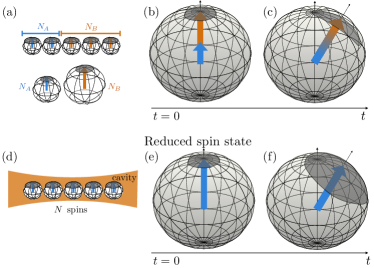
Figure 1: Illustration of the temporal growth of quantum fluctuations and the associated entanglement generation in spin systems with direct interactions (a-c) or with interactions mediated by bosonic “cavity” modes (d-f). The collective spin can be represented through an extended grey region on the Bloch sphere surrounding the point identified by its average polarization $\braket{\hat{\mathbf{S}}(t)}$. The grey region represents the uncertainty of the collective spin polarization due to quantum fluctuations. Top panels (a-c): spin-spin interactions lead to a progressive stretching of the spin fluctuations, or spin squeezing, which determines the growth of bipartite (between subsets of spins $A$ and $B$) and of multipartite entanglement. Bottom panels (d-f): the entanglement between the spins and the bosonic cavity mode can be read out from the area covered by spin fluctuations on the Bloch sphere.

III Models

In this introductory section, we briefly recall the well-known properties of quantum many-particle systems with collective interactions, with emphasis on their limiting semiclassical description. We then describe the initial states considered throughout this work. We conclude by introducing two paradigmatic models belonging to this class, which will be used to illustrate our analysis: the quantum kicked top and the Dicke model. This section mostly reviews standard material in the literature.

III.1 Collective quantum many-body systems

We recall how the permutational symmetries allow for exactly mapping collective quantum models to systems of few degrees of freedom characterized by a vanishingly small effective Planck’s constant in the thermodynamic limit Sciolla and Biroli (2011).

We consider an Hamiltonian $\hat{H}$ characterizing a uniform all-to-all interaction of $N$ elementary constituents, such as spins or particles. The symmetry under permutations of the degrees of freedom makes the mean-field treatment of the quantum dynamics exact for large $N$. To show how the semiclassical description emerges, we consider an ensemble of $N$ identical $q$-level quantum systems. A basis of the many-body Hilbert space can be constructed as the tensor product of identical single-unit bases $\{\Ket{\alpha}\}$ with $\alpha=1,\dots,q$. Typical states prepared in experiments may be simple products of identical single-body states, or ground states. Such states generally belong to the totally-symmetric subspace (TSS) of the many-body Hilbert space simultaneously invariant under all permutations . Due to the symmetry of $\hat{H}$, the time-evolved state never leaves the TSS. A basis of the TSS can be labeled by the numbers $N_{1},\dots,N_{q}$ of units occupying each level $\alpha=1,\dots,q$ (with $\sum_{\alpha=1}^{q}N_{\alpha}=N$). The dimension of the TSS,

$$\text{dim TSS }=\binom{N+q-1}{q-1}\quad\underset{N\to\infty}{\thicksim}\quad\frac{N^{q-1}}{(q-1)!}\ ,$$ (2)

is only polynomially large in $N$, which allows for the exact numerical analysis of large systems. It was shown by Sciolla and Biroli in Ref.Sciolla and Biroli (2011) that the dynamics of symmetric observables within the TSS is semiclassical in the thermodynamic limit. This result is based on the smoothness of the matrix elements of $\hat{H}$ between two TSS states with respect to small changes in the occupation numbers $N_{\alpha}\to N_{\alpha}\pm 1,\pm 2,\dots$ (see Appendix A for details). The Schrödinger equation for the TSS wavefunction is governed by the effective Hamiltonian $\hat{H}=N\,\mathcal{H}_{\text{cl}}(\hat{\mathbf{q}},\hat{\mathbf{p}})$ expressed in terms of the conjugated canonical operators

$$\frac{N_{\alpha}}{N}\mapsto\hat{q}_{\alpha},\qquad-i\frac{\partial}{\partial N_{\alpha}}\mapsto\hat{p}_{\alpha}\ ,$$ (3)

with an effective Planck’s constant

$$\hbar_{\text{eff}}\equiv\frac{1}{N}\qquad\text{($\hbar=1$ in our units)}\ ,$$ (4)

that approaches zero in the thermodynamic limit. Thus, the quantum dynamics of the original system of all-to-all interacting $q$-level units starting from a quasiclassical state, is equivalent to the semiclassical dynamics of $n=q-1$ collective degrees of freedom, governed by the Hamilton equations generated by $\mathcal{H}_{\text{cl}}$.

A more detailed discussion of the dynamics of quantum fluctuations around the classical limit, and of the range of validity of the semiclassical description, will be reviewed in Sec.V below.

III.2 Infinite-range spin systems

In the specific case a system of $N$ interacting spins-$1/2$ or qubits, the limiting semiclassical description can be formulated in a more direct and intuitive way, by considering that the TSS coincides with the Dicke manifold of maximal collective spin $S=N/2$, whereby the behavior of collective spin operators approaches the classical limit. In fact, consider general spin models with arbitrary all-to-all multi-body interactions, described by a Hamiltonian of the form

$$\hat{H}=-\sum_{p=1,2,\dots}\Bigg{\{}\sum_{\mu_{1},\dots,\mu_{p}=x,y,z}\frac{J_{\mu_{1}\dots\mu_{p}}}{N^{p-1}}\sum_{i_{1}\neq\dots\neq i_{p}}^{N}\hat{s}^{\mu_{1}}_{i_{1}}\dots\hat{s}^{\mu_{p}}_{i_{p}}\Bigg{\}}$$ (5)

where $\mathbf{\hat{s}}_{i}$, $i=1,2,\dots,N$ are quantum spins-$s$. The rescaling factor $1/N^{p-1}$ is such that the energy contribution of all $p$-body interactions is extensive. These Hamiltonians can be written in terms of the collective spin of the system

$$\mathbf{\hat{S}}=\sum_{i=1}^{N}\mathbf{\hat{s}}_{i}\ ,$$ (6)

as

$$\frac{\hat{H}}{N}=-\sum_{p\geq 1}\Bigg{\{}\frac{1}{N^{p}}\sum_{\mu_{1},\dots,\mu_{p}=x,y,z}J_{\mu_{1}\dots\mu_{p}}\;\hat{S}^{\mu_{1}}\dots\,\hat{S}^{\mu_{p}}\Bigg{\}}\ .$$ (7)

The collective spin’s magnitude $\lvert\mathbf{\hat{S}}\rvert=\sqrt{S(S+1)}$ with $S=Ns,Ns-1,Ns-2,\dots$ is extensive and conserved, $\Big{[}\lvert\mathbf{\hat{S}}\rvert^{2},\hat{H}\Big{]}=0$. The ground state typically belongs to the maximal total spin sector, characterized by the maximal spin projection $S=Ns$ (see, e.g., Ref.Vidal et al. (2004)).

For such states with maximal spin, the thermodynamic limit $N\to\infty$ is equivalent to the semiclassical limit, or, in loose terms, to a classical continuous spin $\langle\mathbf{\hat{S}}\rangle/N$ of (conserved) length $s$. In fact, these reduced spin variables satisfy a commutation relation of the form $\big{[}\hat{S}^{\mu}/N,\hat{S}^{\nu}/N\big{]}=(i/N)\;\epsilon_{\mu\nu\rho}\;\hat{S}^{\rho}/N$, whence one sees that Eq.(7) defines a semiclassical system with an effective Planck’s constant $\hbar_{\text{eff}}\equiv 1/N$ which vanishes in the thermodynamic limit $N\to\infty$. The limiting classical Hamiltonian $\hat{H}/N\to\mathcal{H}_{\text{cl}}$ thus reads

$$\mathcal{H}_{\text{cl}}(\vec{\mathcal{S}})=-\sum_{\mu_{1}}J_{\mu_{1}}\;\mathcal{S}^{\mu_{1}}-\sum_{\mu_{1},\mu_{2}}J_{\mu_{1}\mu_{2}}\;\mathcal{S}^{\mu_{1}}\mathcal{S}^{\mu_{2}}-\dots\ ,$$ (8)

where now $\mathbf{\hat{S}}/N\to\vec{\mathcal{S}}$ represents a classical spin on the sphere of radius $s$ which can be parametrized by spherical coordinates: choosing the $z$ direction as the polar axis, $\vec{\mathcal{S}}=s\hat{\mathbf{Z}}$ with

$$\hat{\mathbf{Z}}=\,\begin{pmatrix}\sin\theta\cos\phi\\ \sin\theta\sin\phi\\ \cos\theta\end{pmatrix}\ .$$ (9)

The rigorous meaning of the classical limit is that, as ${N\to\infty}$, the ground state expectation values $\braket{\mathbf{\hat{S}}}_{\text{GS}}/N$ of the spin components converge to the minimum point $\vec{\mathcal{S}}^{*}$ of the classical Hamiltonian $\mathcal{H}_{\text{cl}}$ on the sphere, with vanishingly small quantum fluctuations, and their nonequilibrium evolution $\braket{\mathbf{\hat{S}}(t)}/N$ upon varying in time some parameter $J=J(t)$ in the Hamiltonian is described by the classical trajectory $\vec{\mathcal{S}}(t)$ on the sphere governed by $\mathcal{H}_{\text{cl}}$, i.e., $\dot{\vec{\mathcal{S}}}=\big{\{}\vec{\mathcal{S}},\mathcal{H}_{\text{cl}}\big{\}}$, with the Poisson brackets $\{\mathcal{S}^{\mu},\mathcal{S}^{\nu}\}=\epsilon_{\mu\nu\rho}\mathcal{S}^{\rho}$. This time-evolution can be recast in terms of the spherical angles $\theta(t),\,\phi(t)$ defined in Eq.(9).

If $s>1/2$, a permutationally invariant Hamiltonian may feature additional “self-interaction” terms with ${j_{1}=j_{2}}$ in Eq.(5), e.g., energy contributions proportional to $\sum_{j=1}^{N}(\hat{s}_{j}^{z})^{2}$. Such terms break the conservation of the collective spin magnitude. In this case the dynamics take place in the full TSS, which is strictly larger than the Dicke manifold, in agreement with the general mapping of Ref.Sciolla and Biroli (2011) reviewed above.

III.3 Beyond global permutational symmetry

The semiclassical approach reviewed in the previous Secs.III.1 and III.2 applies to a much wider class of states and models than discussed therein.

One natural extension consists of a composite system of $M$ collective subsystems, possibly composed of different kinds of degrees of freedom. Provided the interactions couple the various subsystems uniformly in their elementary units, i.e., via collective operators only, the global system has a semiclassical description. In fact, when each subsystem is large, the global system will be described by $\sum_{m=1}^{M}(q_{m}-1)$ semiclassical collective degrees of freedom. The Dicke model, where $N$ spins interact collectively with a cavity mode (see also Sec.III.6 below), can be viewed as an example, as well as the two-species kicked top Miller and Sarkar (1999b).

A second, closely related generalization, is represented by non-symmetric states which partially break the full permutational symmetry. Such states may be obtained by bringing together a number $M\ll N$ of initially separated subsystems. In this case, the full permutational symmetry breaks down into the product of smaller permutational symmetries acting separately on each subsystem. While the full system evolves outside of its TSS, the restricted symmetry allows a description of the dynamics within the product of the TSSs of the $M$ individual subsystems. The semiclassical theory can thereby be applied in the thermodynamic limit, and one ends up with a few-body semiclassical system described by $M\times(q-1)$ collective degrees of freedom. In this case, the Hamiltonian depends on these variables only via the $q-1$ global collective combinations, leaving all the $(M-1)\times(q-1)$ remaining coordinates frozen in their initial values. A simple example is given by a permutationally invariant system of $N$ spins-$1/2$ initially in a random product state $\left|\dots\nearrow\nearrow\nearrow\swarrow\nearrow\swarrow\swarrow\nearrow\dots\right\rangle$ of spins pointing up or down along a given axis. Such a state is far away from the Dicke manifold of maximal total spin length $N/2$. Grouping together the spins pointing in the same direction into two subsystems $A$ and $B$, with $N_{A}$ and $N_{B}$ spins respectively, the global system may be viewed as two interacting collective spins $\hat{\mathbf{S}}_{A}$, $\hat{\mathbf{S}}_{B}$, of length $N_{A}/2$ and $N_{B}/2$ respectively, initially pointing in opposite directions. In agreement with the above observation, the motion of the the two spins is not independent: the Hamiltonian generates a nonlinear collective precession, and the angle between $\hat{\mathbf{S}}_{A}$ and $\hat{\mathbf{S}}_{B}$ is a constant of motion.

III.4 Quasiclassical initial states

We consider systems initialized in pure nonentangled states, such as uncorrelated product states. These states are routinely prepared in cold-atom experiments via standard techniques. In systems described by interacting spins, a natural class of nonentangled states is given by fully polarized states, in which all spins point along a common direction. For composite systems, we will consider uncorrelated products of coherent states. Weakly entangled initial states may be treated on equal footing.

Such initial states have a semiclassical nature, as their classical phase-space representations via the Wigner function Littlejohn (1986); Polkovnikov (2010) correspond to narrow Gaussian distributions centered around a point with a small variance of quantum fluctuations of order $\mathcal{O}(\hbar_{\text{eff}})$. For example, a system of $N$ spins fully polarized in the $z$ direction has

$$\left\langle\frac{\hat{\mathbf{S}}}{N}\right\rangle=s\,\begin{pmatrix}0\\ 0\\ 1\\ \end{pmatrix}\ ,\quad\left\langle\frac{\delta\hat{\mathbf{S}}^{2}}{N^{2}}\right\rangle={\frac{1}{2}}s\,\begin{pmatrix}\hbar_{\text{eff}}\\ \hbar_{\text{eff}}\\ 0\\ \end{pmatrix}\ ,$$ (10)

(with $\delta\hat{\mathbf{S}}=\hat{\mathbf{S}}-\braket{\hat{\mathbf{S}}}$), i.e., the collective spin fluctuations in the transverse directions are vanishingly small. The phase-space representation is this state is given by the Bloch sphere portrait in Fig.1 (b,e). More generally, quasiclassical states can be characterized as Gaussian phase-space distributions centered around a point $\big{(}\mathbf{q}_{\text{cl}},\mathbf{p}_{\text{cl}}\big{)}\equiv\big{(}\braket{\hat{\mathbf{q}}},\braket{\hat{\mathbf{p}}}\big{)}$, with a width of order $\hbar_{\text{eff}}$ per degree of freedom. Ground states of collective models are typically in this class (see, e.g., Refs.Sciolla and Biroli (2011); Vidal et al. (2004)).

According to the standard semiclassical theory Littlejohn (1986); Brack and Bhaduri (1997); Polkovnikov (2010), quantum fluctuations around the classical trajectory $\big{(}\mathbf{q}_{\text{cl}}(t),\mathbf{p}_{\text{cl}}(t)\big{)}$ will remain approximately Gaussian for a diverging time scale as $\hbar_{\text{eff}}\to 0$ (the so-called Ehrenfest time scale) during the evolution. This will be further discussed in Sec.V.4.

III.5 The quantum kicked top

As a first illustrative model, we consider a driven model: the quantum kicked top. The latter can be defined as an ensemble of quantum spins in a magnetic field periodically kicked via collective interactions. The model is described by the Hamiltonian

$$\hat{H}(t)=\alpha\hat{S}_{x}+\frac{\beta}{2Ns}\,\hat{S}_{z}^{2}\sum_{n=-\infty}^{\infty}\delta(t-n\tau)\ ,$$ (11)

where $\hat{S}_{x,y,z}$ are the collective spin operators in Eq.(6) and $\tau$ the period of the periodic kicking. We fix $\tau=1$. Depending on the value of the kicking strength $\beta$, this model is known to exhibit a transition between a regular regime and a chaotic one Haake et al. (1987); Haake (2010). Being a paradigmatic model for quantum chaotic behavior, its bipartite Zarum and Sarkar (1998); Miller and Sarkar (1999b); Chaudhury et al. (2009); Ghose and Sanders (2004); Piga et al. (2019); Wang et al. (2004); Trail et al. (2008); Ghose et al. (2008); Kumari and Ghose (2019); Lombardi and Matzkin (2011); Stamatiou and Ghikas (2007), multipartite entanglement Ghose et al. (2008); Madhok et al. (2014); Fiderer and Braun (2018); Pappalardi et al. (2018) and scrambling dynamics Pappalardi et al. (2018); Sieberer et al. (2019); Pilatowsky-Cameo et al. (2020) have been intensively explored.

The stroboscopic time-evolution operator (namely, the time-evolution operator over one period) encodes the dynamical stability properties — regularity or chaos — of the system. It can be written as

$$\hat{U}=\hat{U}_{\beta}\hat{U}_{\alpha}\quad\text{with}\,\,\hat{U}_{\alpha}=e^{-i\alpha\hat{S}^{x}},\,\,\hat{U}_{\beta}=e^{-i\frac{\beta}{2Ns}(\hat{S}^{z})^{2}}\ .$$ (12)

Due to the collective nature of the interactions, for large $N$ the classical limit is approached. In this limit, the stroboscopic evolution from time $t=n$ to $t=n+1$ can be expressed as a discrete map on the Bloch sphere. This is obtained as the composition of the two following transformations

$$\begin{dcases}\phi^{\prime}=\arctan\left[\tan\phi\cos\alpha-\frac{\sin\alpha}{\tan\theta\cos\phi}\right]+\pi\,H(-\cos\phi)\\ \cos\theta^{\prime}=\cos\theta\cos\alpha+\sin\theta\sin\phi\sin\alpha\ ,\end{dcases}$$ (13a)

$$\begin{dcases}\phi^{\prime\prime}=\phi^{\prime}+\beta\cos\theta^{\prime}\\ \cos\theta^{\prime\prime}=\cos\theta^{\prime}\end{dcases}\ ,$$ (13b)

where $H(x)$ is the Heaviside step function. See Appendix B.1 for the derivation.

III.6 The Dicke model

As a second illustrative example, we consider a conservative system: the Dicke model. The latter was originally defined Dicke (1954) as an ensemble of two-level atoms collectively interacting with a single mode of the quantized electromagnetic field. Representing the atoms as spins-$1/2$, one can write the Dicke Hamiltonian as

$$\hat{H}=\omega_{0}\hat{S}^{z}+\omega\hat{b}^{\dagger}\hat{b}+\frac{\gamma}{\sqrt{N}}\frac{\hat{b}^{\dagger}+\hat{b}}{\sqrt{2}}\hat{S}^{x},$$ (14)

where $\hat{S}^{x,y,z}$ are spin-$1/2$ collective operators as in Eq.(6) and $\hat{b}^{\dagger}$, $\hat{b}$ are creation and annihilation operators of a bosonic mode. For convenience, we define the real quadrature operators $\hat{Q}=(1/\sqrt{2})(\hat{b}+\hat{b}^{\dagger})$, $\hat{P}=(1/i\sqrt{2})(\hat{b}-\hat{b}^{\dagger})$. The Dicke model has interesting equilibrium and nonequilibrium properties. At zero temperature, the system undergoes a phase-transition at $\gamma_{c}=\sqrt{\omega\omega_{0}}/2$, between a normal phase $(\gamma<\gamma_{c})$ to a super-radiant one $(\gamma>\gamma_{c})$ Dicke (1954). Furthermore, in the classical limit the accessible phase space may undergo a progressive regular-to-chaotic transition upon varying the energy $E$ and/or the coupling $\gamma$ Emary and Brandes (2003); de Aguiar et al. (1992). Its bipartite Furuya et al. (1998); Lambert et al. (2004); Lóbez and Relaño (2016); Sinha and Sinha (2019); Lewis-Swan et al. (2019), multipartite entanglement Song et al. (2012); Wang et al. (2014); Zhang and Chen (2015); Mirkhalaf and Smerzi (2017); Gietka et al. (2019); Bhattacherjee and Sharma (2016); Lewis-Swan et al. (2019) and scrambling dynamics Buijsman et al. (2017); Alavirad and Lavasani (2019); Chávez-Carlos et al. (2019); Lewis-Swan et al. (2019) have been intensively explored.

The dynamics of the Dicke model approach their classical limit for ${N\to\infty}$, described by the classical Hamiltonian ${\hat{H}/N\to\mathcal{H}_{\text{cl}}}$

$$\mathcal{H}_{\text{cl}}=\omega_{0}\mathcal{S}^{z}+\omega\frac{\mathcal{Q}^{2}+\mathcal{P}^{2}}{2}+\gamma\mathcal{Q}\mathcal{S}^{x}\ ,$$ (15)

with

$$\hat{\mathbf{S}}\thicksim\frac{N}{2}\;\mathbf{Z}(t)\ ,\quad\hat{Q}\thicksim\sqrt{N}\mathcal{Q}(t)\ ,\quad\hat{P}\thicksim\sqrt{N}\mathcal{P}(t)\ ,$$ (16)

where $\mathbf{Z}(t)$ represents the direction of the average collective spin and it is parametrized by the time-dependent angles $\phi(t),\,\theta(t)$ [cf. Eq.(9)]. The functions $\mathcal{Q}(t)$, $\mathcal{P}(t)$ describe the limiting classical dynamics of the bosonic mode. The $\sqrt{N}$ scaling may be understood as the occurrence that all terms in the Hamiltonian are extensive and balance each other in equilibrium. The rescaling in Eq.(16) renders the emergence of the effective Planck’s constant $\hbar_{\text{eff}}=1/N$ manifest.

The classical limit of the Hamiltonian governs the coupled dynamics of the atoms and the radiation field via the Hamilton equations

$$\begin{dcases}\dot{\mathcal{Q}}=\omega\mathcal{P}\\ \dot{\mathcal{P}}=-\omega\mathcal{Q}-\frac{\gamma}{2}\sin\theta\cos\phi\\ \dot{\phi}=-\omega_{0}\,\tan\theta+\gamma\mathcal{Q}\,\cos\phi\\ \dot{\theta}=-\gamma\mathcal{Q}\,\sin\phi\end{dcases}\ .$$ (17)

See Appendix B.2 for the derivation.

IV Quantifiers of entanglement and chaos

In this section, we introduce the quantifiers of bipartite and multipartite entanglement and of dynamical chaos, which we will examine in the subsequent analysis.

IV.1 Entanglement entropies

For a composite system with Hilbert space ${\mathcal{H}=\mathcal{H}_{A}\otimes\mathcal{H}_{B}}$ in a pure state $\hat{\rho}=\left|\psi\right\rangle\left\langle\psi\right|$, the bipartite entanglement between subsystems $A$ and $B$ is encoded in the reduced density matrix ${\hat{\rho}_{A}=\operatorname{Tr}_{B}\,{\hat{\rho}}}$ . The system is entangled with respect to the bipartition $(A,B)$ if $\hat{\rho}_{A}$ (equivalently, $\hat{\rho}_{B}$) is not pure. The amount of bipartite entanglement can be quantified by the Renyi entropies

$$S_{A}^{\alpha}=-\frac{1}{1-\alpha}\ln\operatorname{Tr}\hat{\rho}_{A}^{\alpha}\ ,$$ (18)

parameterized by $\alpha>1$. The von Neumann entropy is obtained as their limit for $\alpha\to 1$, i.e.,

$${S_{A}=-\operatorname{Tr}\big{(}\hat{\rho}_{A}\ln\hat{\rho}_{A}\big{)}}\ .$$ (19)

In spatially extended systems with interactions depending on the distance between particles, it is natural to consider bipartitions where subsystem $A$ is constituted by degrees of freedom within a connected region of space, and $B$ its complement. However, in fully-connected $N$-particle systems, the permutational symmetry makes spatial bipartitions meaningless. Hence, we consider bipartitions specified by the number $N_{A}=f_{A}\,N$ of particles in subsystem $A$ (with $N_{B}=N-N_{A}=f_{B}\,N$).

In addition to spatial bipartitions, one can examine bipartitions between different types of degrees of freedom, irrespective of their spatial location. This notion is meaningful in collective models, as well. For instance, for the Dicke model introduced in Sec.III.6, we will focus on the entanglement between the atoms and the cavity field.

For a pictorial representation of the bipartitions considered in this paper, see Fig.1 (a,d).

IV.2 Quantum Fisher information and spin squeezing

A different approach is to characterize the system via the multipartite entanglement properties of the time-evolving state, as given by the quantum Fisher information (QFI) $\mathcal{F}(\hat{O},\hat{\rho})$. This quantity was introduced in metrology to bound the precision of the estimation of a parameter $\phi$, conjugated to an observable $\hat{O}$ using a quantum state $\hat{\rho}$, via the so-called quantum Cramer-Rao bound $\Delta\phi^{2}\geq 1/M\mathcal{F}(\hat{O},\hat{\rho})$, where $M$ is the number of independent measurements made in the protocol Pezzè et al. (2018). The QFI has key mathematical properties Braunstein and Caves (1994); Petz and Ghinea (2011); Tóth and Apellaniz (2014); Pezzè et al. (2018), such as convexity, additivity, monotonicity, and it can be used to probe the multipartite entanglement structure of a quantum state Hyllus et al. (2012); Tóth (2012). If, for a certain $\hat{O}$, the QFI density satisfies the inequality

$$f_{Q}=\frac{\mathcal{F}(\hat{O},\hat{\rho})}{N}>m\ ,$$ (20)

then, at least $(m+1)$ parties in the system are entangled (with $1\leq m\leq N-1$ a divisor of $N$). Namely, $m$ represents the size of the biggest entangled block of the quantum state. In particular, if $N-1\leq f_{Q}(\hat{O})\leq N$, then the state is called genuinely $N$-partite entangled. The QFI has an operational definition in terms of statistical speed of quantum states under external parametric transformations Braunstein and Caves (1994); Wootters (1981). For a general mixed state, described by the density matrix $\hat{\rho}=\sum_{n}p_{n}|n\rangle\langle n|$, it reads Braunstein and Caves (1994)

$${\mathcal{F}}(\hat{O},\hat{\rho})=2\sum_{n,m}\frac{(p_{n}-p_{m})^{2}}{p_{n}+p_{m}}|\langle n|\hat{O}|m\rangle|^{2}{\leq 4\,\langle\Delta\hat{O}^{2}\rangle},$$ (21)

with $\langle\Delta\hat{O}^{2}\rangle=\text{Tr}(\hat{\rho}\,\hat{O}^{2})-\text{Tr}(\hat{\rho}\,\hat{O})^{2}$. The equality holds for pure states $\hat{\rho}=\left|\psi\right\rangle\left\langle\psi\right|$. In general, different operators $\hat{O}$ lead to different bounds and there is no systematic method (without some knowledge on the physical system Hauke et al. (2016); Pezzè et al. (2017)) to choose the optimal one.

In this work, we study the dynamical QFI of pure states out of equilibrium $\left|\psi(t)\right\rangle$. In the case of spin systems of Sec.III.2, we focus on collective spin projections ${\hat{O}=\hat{S}_{\mathbf{n}}=\sum_{i=1}^{N}\mathbf{n}\cdot\mathbf{\hat{s}}_{i}}$ in the direction of the $3d$ unit vector $\mathbf{n}$, while for composite systems we consider $\hat{O}=\mathbb{1}_{\overline{S}}\otimes\hat{S}_{\mathbf{n}}$, where ${\overline{S}}$ is the complement of the spin subsystem. The optimal QFI is then given by the maximal fluctuation of the total spin as

$$f_{Q}(t)=4\max_{\mathbf{n}}\frac{\langle\Delta\hat{S}_{\mathbf{n}}^{2}(t)\rangle}{N}\ .$$ (22)

In the case of composite systems, such as the Dicke model of Sec.III.6, Eq.(22) detects not only the correlations between the individual spins, but also the entanglement between the collective spin and the other degrees of freedom (see e.g., Ref.Gietka et al. (2019)).

A related experimentally relevant indicator of multipartite entanglement in spin systems is given by spin squeezing, a concept first introduced in Ref.Hiroshima (2001). This observable is associated with the reduction of collective spin quantum fluctuations along one direction at the expense of an enhancement of orthogonal fluctuations, due to the Heisenberg principle. Spin squeezing is usually quantified by the minimal transverse variance of collective spin fluctuations Wineland et al. (1992); Ma et al. (2011) as

$$\xi^{2}\equiv\operatorname{Min}_{\lvert\mathbf{u}\rvert=1,\mathbf{u}\perp\mathbf{Z}}\frac{\Big{\langle}\big{(}\mathbf{u}\cdot\mathbf{\hat{S}}\big{)}^{2}\Big{\rangle}}{N/4}.$$ (23)

The squeezing parameter $\xi^{2}$ is equal to $1$ for coherent states, and smaller for squeezed states (see, e.g., Refs. Hiroshima (2001); Ma et al. (2011)). It has long been known Sørensen and Mølmer (2001); Sørensen et al. (2001); Pezzé and Smerzi (2009) that collective spin squeezing is a witness of many-body quantum entanglement. It is possible to demonstrate that $\xi^{2}\geq 1/f_{Q}$ Pezzé and Smerzi (2009), namely there exists a class of states which are not spin-squeezed but can be maximally entangled. In the following, we will show that a simple relation exists between the QFI and spin squeezing in the semiclassical regime.

IV.3 Scrambling and the square commutator

Recently, the study of chaos in quantum systems has received a renewed attention with emphasis on the notion of scrambling. This revival has been triggered by Kitaev’s proposal to characterize quantum chaotic properties in terms of the growth in time of the squared non-equal time commutator of two initially commuting observables Kitaev (2015), i.e.,

$$c(t)=-\langle[\hat{B}(t),\hat{A}]^{2}\,\rangle\ ,$$ (24)

where the expectation value is taken in a generic quantum state $\hat{\rho}$, i.e., $\langle\cdot\rangle=\operatorname{Tr}(\cdot\hat{\rho})$. Note that $c(t)\geq 0$ if $\hat{A}$, $\hat{B}$ are hermitian. This object measures the non-commutativity induced by the dynamics between two initially commuting operators $\hat{A},\hat{B}$ and it contains out-of-time-order correlators $\langle\hat{B}(t)\hat{A}\hat{B}(t)\hat{A}\rangle$, characterized by the absence of time-ordering.

The square commutator was originally introduced in 1969 by Larkin and Ovchinnikov in Ref.Larkin and Ovchinnikov (1969) to describe semi-classically the exponential sensitivity to initial conditions and the associated Lyapunov exponent. In fact, in the classical limit, $c(t)$ encodes the square of the derivatives of the classical trajectory to respect to the initial conditions Cotler et al. (2018). Thus, whenever the classical limit is chaotic, $c(t)$ is expected to grow exponentially in time, with a rate set by twice the classical Lyapunov exponent Jalabert et al. (2018); Rozenbaum et al. (2017); Pappalardi et al. (2018); Chávez-Carlos et al. (2019); Lewis-Swan et al. (2019); Craps et al. (2019); Rozenbaum et al. (2019a); Rammensee et al. (2018); Rautenberg and Gärttner (2019); Prakash and Lakshminarayan (2019); Pappalardi et al. (2020); Craps et al. (2019); Rautenberg and Gärttner (2019); Schmitt et al. (2019); Wang et al. (2019). In this context, several quantum generalizations of the classical Lyapunov spectrum (see below) have been proposed Gharibyan et al. (2019); Rozenbaum et al. (2019b); Yan and Chemissany (2020).

In the present case, we will study the square commutator in Eq.(24) by taking the expectation value in pure quasiclassical initial states introduced in Sec.III.4. In the case of spin systems, we study the square commutator between two collective spin projections (6), namely

$$c_{\alpha\beta}(t)=-\bigg{(}\frac{1}{Ns}\bigg{)}^{2}\left\langle\psi_{0}\right|\left[\hat{S}^{\alpha}(t),\hat{S}^{\beta}(0)\right]^{2}\left|\psi_{0}\right\rangle\ ,$$ (25)

where $\alpha,\beta=x,y,z$ and $\left|\psi_{0}\right\rangle$ is a fully polarized spin-coherent initial state.

IV.4 Lyapunov exponents

Here we recall the definition of the characteristic Lyapunov exponents, while in the Appendix C.1 we report a brief summary of their main properties. We refer the reader to the abundant literature on this topic, e.g., Ref. Cencini et al. (2010).

The notion of deterministic chaos is associated with the strong sensitivity of the evolved state of a system on its initial condition. Given a generic $d$-dimensional flow $\dot{\mathbf{x}}=\mathbf{f}(\mathbf{x})$ in phase space, the measure of the instability of a trajectory $\mathbf{x}(t)$ is provided by the maximum Lyapunov exponent.

Consider an initial condition $\mathbf{x}(0)$ and a neighboring point $\tilde{\mathbf{x}}(0)$ displaced by an infinitesimal amount $\tilde{\mathbf{x}}(0)=\mathbf{x}(0)+\bm{\delta}(0)$. Chaos is defined by an exponential growth in time of the separation between the corresponding trajectories, $\delta(t)=\lvert\tilde{\mathbf{x}}(t)-\mathbf{x}(t)\rvert\thicksim\delta(0)\exp(\lambda t)$, with $\lambda>0$. The rate $\lambda$ generally depends on the initial state and on the observation time $t$. A non-ambiguous definition thus requires “time-averaging”

$$\lambda\coloneqq\lim_{t\to\infty}\;\lim_{\delta(0)\to 0}\;\frac{1}{t}\ln\frac{\delta(t)}{\delta(0)}\ .$$ (26)

The inner limit $\delta(0)\to 0$ translates the (nonlinear) evolution of small displacements away from the initial condition into the (linear) tangential map of the flow along the given trajectory.

The number $\lambda$ above does not exhaust all the possible information on the separation of nearby initial conditions. Consider an infinitesimal hypercube surrounding the initial condition $\mathbf{x}(0)$, identified by $d$ independent infinitesimal displacements $\{\mathbf{w}^{(i)}\}_{i=1}^{d}$, which spans the tangent space at $\mathbf{x}(0)$. The evolution transports this hypercube along the trajectory $\mathbf{x}(t)$, and simultaneously deforms it. The tangent vectors $\{\mathbf{w}^{(i)}\}$ evolve according to the so-called variational equation

$$\dot{\mathbf{w}}(t)=A[\mathbf{x}(t)]\cdot\mathbf{w}(t)\ .$$ (27)

where $A[\mathbf{x}(t)]=\frac{\partial\mathbf{f}}{\partial\mathbf{x}}\big{|}_{\mathbf{x}(t)}$ is usually called the linear stability matrix. The formal solution to this linear equation is

$$\mathbf{w}(t)=U\big{[}\mathbf{x}(t)\big{]}\mathbf{w}(0)$$ (28)

where $U\big{[}\mathbf{x}(t)\big{]}=\mathcal{T}\exp\int_{0}^{t}d\tau\,A[\mathbf{x}(\tau)]$ is the evolution operator, and $\mathcal{T}\exp$ denotes the time-ordered matrix exponential. The deformation of the hypercube in time is captured by inspecting the (positive) eigenvalues $\nu_{1}(t)\geq\nu_{2}(t)\geq\dots\geq\nu_{d}(t)\geq 0$ of the symmetric matrix

$$G(t)=U(t)^{T}\cdot U(t)\ ,$$ (29)

that we refer to as the Oseledets matrix . The asymptotic Lyapunov spectrum is then defined as

$$\lambda_{k}=\lim_{t\to\infty}\frac{1}{t}\ln\sqrt{\nu_{k}(t)}\ .$$ (30)

The existence of this limit for almost all initial data is the content of the celebrated Oseledets multiplicative theorem Oseledets (1968). In particular, one has $\lambda_{1}\equiv\lambda$. In nonergodic dynamics, the numbers $\{\lambda_{k}\}$ may still depend on the particular trajectory.

The Lyapunov spectrum allows one to access the Kolmogorov-Sinai entropy rate $\Lambda_{\text{KS}}$, a fundamental quantifier of irreversibility in dynamical systems. The latter is related to the asymptotic loss of information on the state of the system induced by an arbitrarily fine coarse-graining of the phase space Kolmogorov (1958); Sinai (1959). By Pesin’s theorem Pesin (1977), one has

$$\Lambda_{\text{KS}}=\sum_{k\;:\;\lambda_{k}>0}\lambda_{k}\ .$$ (31)

It is important to stress that the characteristic Lyapunov exponents are defined by a long-time limit [see Eq.(30)]. Accessing the latter may be challenging in numerical simulations. The by now standard algorithm for a robust computation of the Lyapunov spectrum has been proposed by Benettin, Galgani and Strelcyn in a series of papers around 1980 Benettin et al. (1976, 1980a, 1980b). The convergence of the computations is typically quite slow in Hamiltonian systems. This is especially relevant in those undergoing an order/chaos transition, on which we will be concerned in the following. For finite observation-time windows, one naturally defines the local or finite-time Lyapunov exponents $\{\lambda_{k}(t)\}$ as in Eq.(30) without taking the long-time limit. This notion is particularly important in semiclassical dynamics due to the relatively short time window before saturation, as we will extensively discuss in Sec.V.3.

In Appendix C.1, we recall further properties of the Lyapunov spectrum with emphasis on Hamiltonian systems, and in Appendix C.2 we briefly review the algorithm of Benettin et al. in view of its importance later on in this work.

V Relationship between entanglement growth and chaos

In this section, we begin by reviewing how quantum fluctuations evolve around the limiting classical trajectory. We then show how they yield the evolution of $S_{A}(t)$, $f_{Q}(t)$ and $c(t)$ in the semiclassical regime. Hence, we discuss how the dynamics of entanglement and chaos is determined by the structure of the underlying classical phase-space and its chaoticity. Finally, we outline the range of validity of the semiclassical description and discuss the saturation due to finite-size effects.

V.1 Dynamics of quantum fluctuations

As reviewed in Sec.III.1, collective interactions allow for a reformulation of the nonequilibrium dynamics as an effective few-body system in the semiclassical regime, where the impact of quantum fluctuations is controlled by the system size $N$ via the relation $\hbar_{\text{eff}}=1/N$. The generality of this approach has been discussed in Sec.III.3.

A system in this class is thus described by $n$ degrees of freedom, compactly denoted ${\hat{\bm{\xi}}=(\hat{q}_{1},\dots,\hat{q}_{n},\hat{p}_{1},\dots,\hat{p}_{n})}$, satisfying the canonical commutation relations ${[\hat{q}_{i},\hat{p}_{j}]=i\hbar_{\text{eff}}\delta_{ij}}$, or $[\hat{\bm{\xi}},\hat{\bm{\xi}}]=i\hbar_{\text{eff}}\mathbb{J}$. Here we have introduced the symplectic unit $\mathbb{J}$, given by the $2n\times 2n$ antisymmetric matrix $\mathbb{J}={\begin{pmatrix}\mathbb{0}_{n}&\mathbb{1}_{n}\\ -\mathbb{1}_{n}&\mathbb{0}_{n}\end{pmatrix}}$, which satisfies $\mathbb{J}^{2}=-\mathbb{1}_{2n}$. The evolution is governed by the Hamiltonian $\hat{H}=\hbar_{\text{eff}}^{-1}\;\mathcal{H}_{\text{cl}}(\hat{\bm{\xi}})$ and the Heisenberg equations read $\dot{\hat{\bm{\xi}}}=\mathbb{J}\;\partial\mathcal{H}_{\text{cl}}(\hat{\bm{\xi}})$ . As discussed in Sec.III.4, the relevant initial states $\left|\Psi_{0}\right\rangle$ in our study of entanglement dynamics are quasiclassical states, i.e., states which satisfy

$$\braket{\Psi_{0}}{\Big{(}\hat{\bm{\xi}}-\bm{\xi}(0)\Big{)}\Big{(}\hat{\bm{\xi}}-\bm{\xi}(0)\Big{)}}{\Psi_{0}}=\mathcal{O}(\hbar_{\text{eff}})\ ,$$ (32)

with $\bm{\xi}(0)\equiv\braket{\Psi_{0}}{\hat{\bm{\xi}}}{\Psi_{0}}=\mathcal{O}(1)$. The meaning of this condition is that initial quantum fluctuations around the average are of the order of the minimal uncertainty allowed by the Heisenberg principle.

We now aim at describing the evolution of quantum fluctuations around the average. We observe that, by virtue of Eq.(32), the average $\braket{\hat{\bm{\xi}}(t)}$ moves along the classical trajectory to the leading order in $\hbar_{\text{eff}}$,

$$\frac{d}{dt}\braket{\Psi(t)}{\hat{\bm{\xi}}}{\Psi(t)}=\mathbb{J}\;\partial\mathcal{H}_{\text{cl}}\Big{(}\braket{\Psi(t)}{\hat{\bm{\xi}}}{\Psi(t)}\Big{)}+\mathcal{O}(\hbar_{\text{eff}})\ ,$$ (33)

i.e., $\braket{\Psi(t)}{\hat{\bm{\xi}}}{\Psi(t)}=\bm{\xi}_{\text{cl}}(t)+\mathcal{O}(\hbar_{\text{eff}})$. Quantum fluctuations around the average are encoded in the dimensionless variables

$$\delta\hat{\bm{\xi}}\equiv\hbar_{\text{eff}}^{-1/2}\big{(}\hat{\bm{\xi}}-\bm{\xi}_{\text{cl}}(t)\big{)}\ ,$$ (34)

which satisfy the commutation relations $[\delta\hat{\bm{\xi}},\delta\hat{\bm{\xi}}]=i\mathbb{J}$, and, by construction, $\braket{\delta\hat{\bm{\xi}}(t)}=\mathcal{O}(\hbar_{\text{eff}}^{1/2})$ Benatti et al. (2017).

In systems of collectively interacting spins, the quantum fluctuations $\delta\hat{\bm{\xi}}=(\delta\hat{q},\delta\hat{p})$ as in Eq.(34) describe the collective spin fluctuations transverse to the instantaneous spin polarization direction, cf. Sec.III.2. These spin fluctuations can be introduced in the formalism by performing a time-dependent Holstein-Primakoff trasformation around the instantaneous average spin Dusuel and Vidal (2004); Lerose et al. (2018) (see also Lerose et al. (2019a, b); Lerose and Pappalardi (2020)). This standard transformation Wannier (1966) maps the transverse fluctuations of a quantum spin to a canonical bosonic mode. When these fluctuations are small compared to the size of the collective spin, one can approximate the transformation to the quadratic order, obtaining

$$\begin{split}\frac{\hat{S}^{\alpha}}{Ns}&={X}_{\alpha}(t)\,\,\bigg{(}\frac{\hbar_{\text{eff}}}{s}\bigg{)}^{1/2}\,\delta\hat{q}+{Y}_{\alpha}(t)\,\,\bigg{(}\frac{\hbar_{\text{eff}}}{s}\bigg{)}^{1/2}\,\delta\hat{p}\\ &\quad+{Z}_{\alpha}(t)\;\left(1-\bigg{(}\frac{\hbar_{\text{eff}}}{s}\bigg{)}\,\frac{\delta\hat{q}^{2}+\delta\hat{p}^{2}-1}{2}\right)\\ &\quad+\mathcal{O}\left((\hbar_{\text{eff}}/s)^{3/2}\right)\ ,\end{split}$$ (35)

with $\alpha=x,y,z$. Here, the time-dependent unit vector $\mathbf{Z}(t)$ represents the classical dynamics of the collective spin polarization direction. It can be parameterized through the spherical angles $\phi(t)$ and $\theta(t)$ as in Eq.(9). The transverse directions identified by the unit vectors $\mathbf{X}(t),\,\mathbf{Y}(t)$ can be parameterized as

$$\mathbf{X}(t)\equiv\left(\begin{matrix}\cos\theta\cos\phi\\ \cos\theta\sin\phi\\ -\sin\theta\end{matrix}\right),\quad\mathbf{Y}(t)\equiv\left(\begin{matrix}-\sin\phi\\ \cos\phi\\ 0\end{matrix}\right)\ ,$$ (36)

and span the orthogonal space to $\mathbf{Z}(t)$. The short-hand notation in Eq.(35) $X_{\alpha}(t)$, $Y_{\alpha}(t)$, $Z_{\alpha}(t)$ denotes the $\alpha$-th components of the basis vectors $\mathbf{X}(t)$, $\mathbf{Y}(t)$, $\mathbf{Z}(t)$ in Eqs.(9) and (36) (i.e., $X_{z}=-\sin\theta$, $Y_{z}=0$, $Z_{z}=\cos\theta$, …). One can check that the bosonic operators $\delta\hat{q},\delta\hat{p}$ introduced via the Holstein-Primakoff transformation, correspond to the rescaled fluctuations $\delta\hat{\bm{\xi}}$ introduced above for the collective spin when the Bloch sphere is parametrized through the canonical phase-space variables $q=\phi$ and $p=\cos\theta$. When the system comprises $M>1$ collective spins, of magnitude $N_{j}s\gg 1$, $j=1,\dots,M$, one can perform the analogous transformation (35) on their components $\hat{S}^{\alpha}_{j}$ to obtain the joint semiclassical description.

The general transformation (34) is time-dependent. The exact evolution equations for the quantum fluctuations $\delta\hat{\bm{\xi}}$ are thus generated by the modified Hamiltonian

$$\hat{\widetilde{H}}(t)=\hbar_{\text{eff}}^{-1}\;\mathcal{H}_{\text{cl}}\Big{(}\bm{\xi}_{\text{cl}}(t)+\hbar_{\text{eff}}^{1/2}\delta\hat{\bm{\xi}}\Big{)}-\hbar_{\text{eff}}^{-1/2}\;\dot{\bm{\xi}}_{\text{cl}}(t)\,\mathbb{J}\,\delta\hat{\bm{\xi}}\ .$$ (37)

We can now expand the Hamiltonian with respect to the small parameter $\hbar_{\text{eff}}$, obtaining the time-dependent Hamiltonian

$$\hat{\widetilde{H}}(t)\,=\,\hbar_{\text{eff}}^{-1}\;\hat{{H}}_{0}(t)\,+\,\hbar_{\text{eff}}^{-1/2}\;\hat{{H}}_{1}(t)\,+\,\hat{{H}}_{2}(t)\,+\,\mathcal{O}(\hbar_{\text{eff}}^{1/2})\ .$$ (38)

Here, $\hat{{H}}_{0}(t)=\mathcal{H}_{\text{cl}}\big{(}\bm{\xi}_{\text{cl}}(t)\big{)}$ is just a classical quantity (the classical energy along the classical trajectory), and the linear term $\hat{{H}}_{1}(t)=\Big{[}\partial\mathcal{H}_{\text{cl}}\big{(}\bm{\xi}_{\text{cl}}(t)\big{)}-\dot{\bm{\xi}}_{\text{cl}}(t)\mathbb{J}\Big{]}\delta\hat{\bm{\xi}}$ vanishes identically by construction, consistently with the vanishing of $\braket{\delta\hat{\bm{\xi}}(t)}$ to the leading order in $\hbar_{\text{eff}}$. The operator expansion thus starts from the (finite) quadratic order. Within the semiclassical regime, and for a time scale that diverges as $\hbar_{\text{eff}}\to 0$ (the so-called Ehrenfest time scale, see below), we can neglect the remainder $\mathcal{O}(\hbar_{\text{eff}}^{1/2})$ in the expansion. The evolution of the quantum fluctuations in this regime is determined by a linear homogeneous differential equation,

$$\frac{d}{dt}\delta\hat{\bm{\xi}}=A(t)\;\delta\hat{\bm{\xi}}\equiv\mathbb{J}\,\partial^{2}\mathcal{H}_{\text{cl}}\big{(}\bm{\xi}_{\text{cl}}(t)\big{)}\;\delta\hat{\bm{\xi}}\ ,$$ (39)

identical with the classical variational equation for the evolution of infinitesimal displacements away from the classical trajectory [cf. Sec.IV.4 Eq.(27)]. In fact, the classical and quantum evolutions generated by a quadratic Hamiltonian coincide, as is well known.

The solution to this equation is formally written as

$$\begin{split}\delta\hat{\bm{\xi}}(t)&=U(t)\;\delta\hat{\bm{\xi}}(0)\ ,\end{split}$$ (40)

where $U(t)\equiv\mathcal{T}\exp\int_{0}^{t}d\tau\,A(\tau)$ is the tangential map, which encodes the evolution of infinitesimal classical displacements. Due to the asymptotic Gaussian description for small $\hbar_{\text{eff}}$, all the information on the quantum state is encoded in the correlation matrix

$$[G(t)]_{ij}=\frac{1}{2}\braket{\Psi(t)}{\delta\hat{\xi}_{i}\,\delta\hat{\xi}_{j}+\delta\hat{\xi}_{j}\,\delta\hat{\xi}_{i}}{\Psi(t)}\ ,$$ (41)

with $i,j=1,\dots,2n$. This matrix is symmetric and positive definite; the square root of its eigenvalues quantify the width of the quantum fluctuations around the classical average, and are constrained from below by the Heisenberg principle (see, e.g., Ref. Littlejohn (1986)). Notice that the rescaling by $\hbar_{\text{eff}}^{1/2}$ in Eq.(32) is equivalent to the statement that $G(t)=\mathcal{O}(1)$. The evolution of the correlation matrix $G(t)$ can be directly expressed via Eq.(40) as

$$G(t)=U(t)^{T}\;G(0)\;U(t)\ .$$ (42)

V.2 Semiclassical expressions of entanglement and chaos quantifiers

In this section we will analytically derive the relation between the entanglement quantifiers of Sec.IV and the chaos indicators in the semiclassical regime.

V.2.1 Semiclassical entanglement entropies

We consider a quantum collective model and introduce a bipartition $(A,B)$ of its degrees of freedom as discussed in Sec.IV.1. Within the semiclassical description, the bipartite system can be represented by two sets of semi-classical variables $\hat{\bm{\xi}}=(\hat{\bm{\xi}}_{A},\hat{\bm{\xi}}_{B})$, with $n_{A}$ and $n_{B}$ collective degrees of freedom, respectively ($n_{A}+n_{B}=n$) . In this regime, the entanglement between the two subsystems is encoded in the entanglement between their bosonic quantum fluctuations $\delta\hat{\bm{\xi}}_{A}$, $\delta\hat{\bm{\xi}}_{B}$. The extent of these quantum fluctuations is collected in their correlation matrix $G(t)$ in Eqs. (41)-(42). It is convenient to define the subsystem reduced correlation matrix $G_{A}(t)$ as the $2n_{A}\times 2n_{A}$ sub-matrix of $G(t)$ built out of the coordinates of subsystem $A$ alone, i.e.,

$$[G_{A}(t)]_{ij}=\frac{1}{2}\braket{\Psi(t)}{\delta\hat{\xi}_{i}\,\delta\hat{\xi}_{j}+\delta\hat{\xi}_{j}\,\delta\hat{\xi}_{i}}{\Psi(t)}_{\begin{subarray}{c}1\leq i\leq 2n_{A}\\ 1\leq j\leq 2n_{A}\end{subarray}}\ .$$ (43)

Due to the asymptotic Gaussian description for small $\hbar_{\text{eff}}$, the reduced density matrix $\hat{\rho}_{A}(t)$ is also Gaussian and fully determined by the matrix $G_{A}(t)$. The entanglement entropies can thus be computed via standard techniques Vidal J. and Barthel (2007).

The dynamics of the entanglement entropies in bosonic systems governed by quadratic Hamiltonians has been derived and discussed in full generality in Refs. Bianchi et al. (2018); Hackl et al. (2018). It is shown therein, that the second Renyi entropy (18) can be expressed as the logarithm of the phase-space volume spanned by the time-evolving phase-space distribution associated with the reduced state of the subsystem, i.e.,

$$S^{(2)}_{A}(t)=\frac{1}{2}\ln\;\det\big{(}2G_{A}(t)\big{)}\ .$$ (44)

While the global evolution preserves the total volume, i.e., $\det\big{(}2G(t)\big{)}\equiv 1$, the information loss generated by projecting the collective quantum fluctuations onto a subsystem with $n_{A}<n$ yields an increase of entropy, whose origin is rooted in the development of quantum entanglement. By Eq.(44), this increase may be visualized as an enhancement of the projected volume spanned by the reduced quantum fluctuations within the subsystem’s phase space, due to the progressive stretching of the global phase-space volume spanned by the quantum fluctuations. Similarly, the von Neumann entanglement entropy (19) can be computed as

$$\begin{split}S_{A}(t)=\sum_{i=1}^{n_{A}}S(\nu_{i}(t))&\quad\text{with}\\ S(\nu)=\frac{\nu+1}{2}&\ln\frac{\nu+1}{2}-\frac{\nu-1}{2}\ln\frac{\nu-1}{2}\ ,\end{split}$$ (45)

where $\pm\nu_{i}(t)$ ($\nu_{i}(t)\geq 1$) are the so-called symplectic eigenvalues of $2G_{A}(t)$ . The entanglement entropy $S_{A}(t)$ is bounded above and below by the second Renyi entropy up to a constant, and hence their growths are superimposed after a finite transient, $S_{A}(t)\underset{t\gg 1}{\thicksim}S^{(2)}_{A}(t)$, see Ref.Bianchi et al. (2018). Their common asymptotic behavior generically depends on the subsystem only via its number $n_{A}$ of degrees of freedom, and their evolution is completely determined by that of $G(t)$.

As discussed in Sec.IV.1, in many interesting semi-classical models, the relevant subsystem $A$ is made of only one collective degree of freedom, i.e., $n_{A}=1$. These include both the paradigmatic models discussed below, namely the quantum kicked top and the Dicke model. In this case Eq.(45) simplifies and $S_{A}(t)$ can be expressed as a function of the determinant of $G_{A}(t)$, i.e.,

$$\begin{split}S_{A}(t)&=2\sqrt{\det G_{A}}\,\operatorname{arccoth}\left(2\sqrt{\det G_{A}}\right)\\ &\quad+\frac{1}{2}\ln\left(\det G_{A}-\frac{1}{4}\right)\ .\end{split}$$ (46)

From this equation, the asymptotic result of Ref.Bianchi et al. (2018) immediately follows, i.e., $S_{A}(t)\underset{t\gg 1}{\thicksim}\frac{1}{2}\,\ln\;\det G_{A}(t)$, since $\det G_{A}(t){\gg}1$, in agreement with the second Renyi entropy in Eq.(44).

In the case of collective spin systems of the form of Eq.(7), one considers bipartitions between two sets of $N_{A}=f_{A}\,N$ and $N_{B}=f_{B}\,N$ spins ($f_{A}+f_{B}=1$), and a further simplification occurs. By performing a change of variables to the dynamical collective fluctuations and the frozen relative fluctuations of the two spins , it is easy to compute that Lerose and Pappalardi (2020)

$$\det G_{A}=\frac{1}{4}+f_{A}\,f_{B}\langle\hat{n}_{\text{exc}}\rangle\ ,$$ (47)

where $\hat{n}_{\text{exc}}=(\delta\hat{q}^{2}+\delta\hat{p}^{2}-1)/2$ represents the number of bosonic excitations of the collective spin $\mathbf{\hat{S}}$. This allows to compute $S_{A}(t)$ in a closed form, without the need to compute the reduced correlation matrix $G_{A}(t)$ Lerose and Pappalardi (2020); Homrighausen and Kehrein (2019). It is then clear that $S_{A}$ vanishes for $\langle\hat{n}_{\text{exc}}\rangle\to 0$ and grows as $\frac{1}{2}\ln\langle\hat{n}_{\text{exc}}\rangle$ for $\langle\hat{n}_{\text{exc}}\rangle\gg 1$. Hence, Eqs.(46-47) clarify that the state of subsystem $A$ (or $B$) is pure only if $\langle\hat{n}_{\text{exc}}\rangle=0$, i.e., if the spin system is fully polarized (coherent), as occurs in the absence of interactions. Conversely, the state is entangled in the presence of collective quantum excitations.

As we will see in the next sections, the entanglement entropy of a collective spin system can been quantitatively related to the quantum Fisher information and to the spin squeezing.

V.2.2 Semiclassical quantum Fisher information and spin squeezing

The quantum Fisher information for collective spin systems is given by the maximal variance of the collective spin operators [cf. Eq.(22)]. This information is encoded in the correlation matrix $G(t)$ (41), which describes the dynamics of the fluctuations in the transverse direction. Therefore, the semiclassical QFI is given by the maximum eigenvalue of the correlation matrix $G(t)$

$$f_{Q}(t)=4\operatorname{Max}\left[\text{Eigvals}\,G(t)\right]\ .$$ (48)

In the case of a fully-connected spin system (Sec.III.2), one can determine the QFI explicitly, by computing the eigenvalue of the $2\times 2$ spin correlation matrix. This yields the equation

$$f_{Q}(t)=1+2\langle\hat{n}_{\text{exc}}(t)\rangle+2\sqrt{\langle\hat{n}_{\text{exc}}(t)\rangle(\langle\hat{n}_{\text{exc}}(t)\rangle+1)}\ ,$$ (49)

where $\langle\hat{n}_{\text{exc}}(t)\rangle$ is the number of bosonic excitations of the collective spin $\mathbf{\hat{S}}$ [cf. Eqs.(35) and (47)].

As discussed in Sec.IV.2, spin squeezing represents a convenient indicator of multipartite entanglement in spin systems. At the semiclassical level relevant here, quantum fluctuations are Gaussian, and one derives Weedbrook et al. (2012)

$$\xi^{2}(t)=1+2\langle\hat{n}_{\text{exc}}(t)\rangle-2\sqrt{\langle\hat{n}_{\text{exc}}(t)\rangle(\langle\hat{n}_{\text{exc}}(t)\rangle+1)}\;.$$ (50)

Equations (46-47), (49) and (50) express the quantitative link — pictorially illustrated in Fig.1 — between the entanglement entropy $S_{A}$, the quantum Fisher information $f_{Q}$, and the spin squeezing parameter $\xi$, in collective spin models in the semiclassical regime in and out of equilibrium. In particular, in this regime the inequality discussed in Sec.IV.2 is saturated, i.e., $f_{Q}=1/\xi^{2}$.

V.2.3 Semiclassical square commutator

Along similar lines, we can compute the semiclassical evolution of the out-of-time-order square commutator defined in Sec.IV.3 for a system initialized in a quasiclassical state. Starting from the definition in Eq.(24) and expanding the operators up to the quadratic order in the quantum fluctuations, one readily finds

$$\begin{split}c_{ij}(t)&\equiv-{\hbar_{\text{eff}}^{-2}}\braket{\Psi_{0}}{\Big{[}\hat{\xi}_{i}(t),\hat{\xi}_{j}(0)\Big{]}^{2}}{\Psi_{0}}\\ &=\Big{(}U_{i\bar{j}}(t)\Big{)}^{2}+\mathcal{O}(\hbar_{\text{eff}}),\end{split}$$ (51)

where $\bar{j}\equiv(j+n)\mod 2n$. The semiclassical square commutator thus directly probes the sensitivity of the classical trajectories to infinitesimal perturbations.

In the case of fully-connected spin systems, the square commutator between two collective spin operators (25) reads

$$\begin{split}c_{\alpha\beta}(t)&=\Big{[}{X}_{\alpha}(t)\big{(}\,U_{qq}(t)\,\,{Y}_{\beta}(0)-U_{qp}(t)\,\,{X}_{\beta}(0)\,\big{)}\\ &\quad\quad+{Y}_{\alpha}(t)\,\big{(}\,U_{pq}(t)\,Y_{\beta}(0)-U_{pp}(t)\,X_{\beta}(0)\,\big{)}\Big{]}^{2}\\ &\quad\quad+\mathcal{O}(\hbar_{\text{eff}})\ ,\end{split}$$ (52)

with the same notation as in Eq.(35). In order to get this result, one first plugs the expansion of the spin operators (35) into the definition (25). Then, after substituting the formal solution for the spin fluctuations at time $t$, i.e., ${\delta\hat{q}(t)=U_{qq}(t)\,\delta\hat{q}(0)+U_{qp}(t)\,\delta\hat{p}(0)}$ and ${\delta\hat{p}(t)=U_{pq}(t)\,\delta\hat{q}(0)+U_{pp}(t)\,\delta\hat{p}(0)}$ [cf. Eq.(40)], the equal-time commutators between the conjugate variables yield the above Eq.(52).

V.3 Entanglement growth and chaos

In the previous section, we have established how the semiclassical dynamics of quantum fluctuations determine the evolution of the entanglement quantifiers of interest, via the time-dependent correlation matrix $G(t)$. This connection highlights that the entanglement growth is determined by the chaoticity properties of the semiclassical dynamics, in turn dictated by the stability of the underlying phase-space trajectories.

The correlation matrix $G(t)$ in Eq.(41) is equivalent to the Oseledets matrix that defines the Lyapunov spectrum in Eq.(30) , as the quantum fluctuations evolve in the same way as the linearized displacements. Hence, the spectrum of the growth rates of the quantum fluctuations encoded in $G(t)$ coincides with the finite-time Lyapunov spectrum $\{\lambda_{k}(t)\}$ of the underlying semiclassical trajectory within the Ehrenfest time scale $T_{\text{Eh}}(N)$, and converges to the proper asymptotic Lyapunov spectrum $\{\lambda_{k}\}$ as $N\to\infty$. On the other hand, for short times, one can consider the limit $t\to 0$ of the above expressions and retrieve the correct early-time expansions, see e.g. Ref.Sorelli et al. (2019).

When the classical dynamics is integrable, the collective motion of the system is orderly and takes place along regular trajectories in phase space, meaning that nearby initial conditions separate linearly in time (generically). This implies that all Lyapunov exponents vanish. This scenario largely persists under weak integrability-breaking Hamiltonian perturbations, as established by KAM theory Pöschel (2009), whereby regular trajectories gradually leave room to chaotic portions of the phase space arising from dynamical resonances. Thus, in integrable or near-integrable semiclassical systems, the temporal growth of the quantum correlations is at most polynomial, $G_{ij}(t)\thicksim t^{2}$, as can be shown explicitly by switching to action-angle variables. Conversely, in systems with far-from-integrable semiclassical dynamics featuring fully developed chaos in phase space, the Lyapunov spectrum is nonvanishing. This implies an asymptotic exponential growth of quantum fluctuations, generically given by $G_{ij}(t)\thicksim e^{2\lambda t}$, where $\lambda$ is the maximal Lyapunov exponent. An immediate consequence of the above observations concerns the asymptotic growth rate of the square commutator. In fact, the latter results to be twice the maximum Lyapunov exponent of the underlying semiclassical dynamics,

$$c(t)\thicksim e^{2\lambda t}.$$ (53)

Crucially, the chaoticity properties of the semiclassical dynamics determine the speed of the entanglement growth, as determined by Eqs.(45) and (48). In fact, by Eq.(48), we immediately derive that the QFI grows as

$$f_{Q}(t)\thicksim e^{2\lambda t}.$$ (54)

The determination of the bipartite entanglement entropies growth requires a more elaborate analysis. In Refs. Bianchi et al. (2018); Hackl et al. (2018) Bianchi, Heykl, et al. discuss the bipartite entanglement dynamics generated by quadratic bosonic Hamiltonians. As thoroughly shown therein, the growth of $S_{A}(t)$ is generically linear in time with a rate set by the sum of the largest $2n_{A}$ Lyapunov exponents,

$$S_{A}(t)\underset{t\gg 1}{\thicksim}S^{(2)}_{A}(t)\thicksim\Lambda_{A}t=\bigg{(}\sum_{k=1}^{2n_{A}}\lambda_{k}\bigg{)}t.$$ (55)

For $n_{A}=n/2$, the rate coincides with the classical Kolmogorov-Sinai entropy rate $\Lambda_{KS}=\sum_{\lambda_{k}\,:\,\lambda_{k}>0}\lambda_{k}$ Kolmogorov (1958); Sinai (1959); Cencini et al. (2010). Analogous equations to the three above apply to the phase-space separatrices when the classical dynamics is integrable; in this case, the Lyapunov spectrum is given by the linearized dynamics around the unstable fixed point on which the trajectory terminates Lerose and Pappalardi (2020); Homrighausen and Kehrein (2019).

By contrast, for generic trajectories, integrable systems have $\Lambda_{KS}=0$. In this case, one has

$$S_{A}(t) \underset{t\gg 1}{\thicksim}S^{(2)}_{A}(t)\thicksim c\ln t\ ,$$ (56a)

$$f_{Q}(t) \thicksim t^{2}\ ,$$ (56b)

$$c(t) \thicksim t^{2}\ ,$$ (56c)

with $c$ an integer.

The classification is concluded by the case of stable equilibrium configurations, the linearized dynamics of which is equivalent to that of coupled harmonic oscillators. Accordingly, all the quantities of interest perform bounded (periodic or quasiperiodic) oscillations. (Note that the same applies to effective linear semiclassical dynamics with suppressed anharmonic contribution, as in the recently discovered mechanism in Refs. Choi et al. (2019); Ho et al. (2019).) A summary of the above discussion is presented in Table 1.

Since quadratic Hamiltonians describe the dynamics of quantum fluctuations around the limiting classical trajectory in the limit $\hbar_{\text{eff}}\to 0$ to the leading order [cf. the discussion in Sec.V.1], Bianchi, Heykl, et al. conjecture that their analysis applies to generic quantum systems in the appropriate semiclassical regime. In particular, $S_{A}(t)\thicksim\Lambda_{A}t$, where $\Lambda_{A}$ is the Kolmogorov-Sinai entropy rate determined by the Lyapunov spectrum as above. It is one of the main purposes of the present work to thoroughly assess this conjecture and firmly establish its range of validity in quantum many-body systems possessing a relevant and controlled semiclassical limit. The asymptotic results of Refs. Bianchi et al. (2018); Hackl et al. (2018) ideally describe the average asymptotic growth at long times. However, typical semiclassical systems generally present strong additional finite-time fluctuations in the entanglement quantifiers. For example, when the limiting classical trajectory is periodic with period $T_{\text{cl}}$, for integrable (chaotic) dynamics one has $T_{\text{cl}}$-periodic oscillations superimposed to the logarithmic (linear) growth of $S_{A}(t)$ and to the polynomial (exponential) growth of $f_{Q}(t)$ and $c(t)$. For general aperiodic classical trajectories, the time-dependence can be much more complicated. These effects can obscure the asymptotic growth until the saturation due to the finite $\hbar_{\text{eff}}$. Accordingly, deviations from the asymptotic result of Refs. Bianchi et al. (2018); Hackl et al. (2018) can be observed.

In Secs.VI and VII below, we will concentrate on systems exhibiting a progressive transition to chaos as a parameter is varied. In such systems, finite-time fluctuations play a major role, due to the complexity of the phase space, featuring a fractal structure of regular trajectories (KAM tori) and chaotic regions. For this reason, the correct semiclassical identification holds between the growth rate of quantum entanglement and the finite-time Lyapunov spectrum $\{\lambda_{k}(t)\}$, rather than the proper asymptotic one. The discrepancy may be particularly severe, due to the relatively short Ehrenfest time scale in chaotic systems. The long-time convergence of the rate of growth of the relevant entanglement and chaos quantifiers to the asymptotic ones compatible with the Lyapunov spectrum competes with their saturation in a finite system at the Ehrenfest time scale $T_{\text{Eh}}(N)\thicksim\ln N$. Hence, the theoretical long-time rates of growth will hardly be accessible in practice. This point is often overlooked in the recent literature on OTOC and its relation to chaos.

We conclude the discussion by commenting that not only the entanglement entropy $S_{A}(t)$ has a finite limit as $\hbar_{\text{eff}}\to 0$, but this limiting quantity has a natural classical interpretation in terms of the loss of information under phase-space coarse-graining during the time-evolution Zurek and Paz (1995); Casati et al. (2012) — which is the meaning of the classical Kolmogorov-Sinai entropy in dynamical systems. It is also interesting to remark that the growth of entanglement entropy in the semiclassical regime is sensitive to the full Lyapunov spectrum, unlike the growth of the OTOCs, which is sensitive to the maximum Lyapunov exponent only.

V.4 Ehrenfest time and finite-size effects

At this stage, it is natural to comment on the time scale of validity of the semiclassical description outlined above. The latter is the well known Ehrenfest time scale, and is estimated as the time at which the size of quantum fluctuations becomes comparable with the typical length in phase space, i.e. $\mathcal{O}(G(t))=\mathcal{O}(\hbar_{\text{eff}}^{-1})$. For orderly, integrable-like motion, quantum fluctuations grow polynomially in time as $G(t)\thicksim t^{2}$, which yields $T_{\text{Eh}}\thicksim\hbar_{\text{eff}}^{-1/2}=\sqrt{N}$. In the presence of unstable, chaotic evolution, instead, one has $G(t)\thicksim e^{2\lambda t}$, where $\lambda$ is the maximum Lyapunov exponent defined in Sec.IV.4. In this case, thus, $T_{\text{Eh}}\thicksim(1/\lambda)\ln\hbar_{\text{eff}}^{-1/2}=(1/2\lambda)\ln N$.

At this time scale, the semi-classical analysis described before breaks down and a full quantum regime takes place, dominated by interference. From the numerical simulations for finite systems, we find that the entanglement descriptors saturate to values compatible with their statistical-mechanical predictions: in particular, we find

$$S_{A}^{\infty}\propto\ln\hbar_{\text{eff}}^{-1}\ ,\quad f_{Q}^{\infty}\propto\hbar_{\text{eff}}^{-1}\ ,$$ (57)

which is also compatible with the results of Sec.V.2.1-V.2.2 evaluated at $T_{\text{Eh}}$. In other words, the asymptotic state is genuinely multipartite entangled $f^{\infty}_{Q}\propto N$, while the bipartite entanglement entropy saturates to $S^{\infty}_{A}\propto\ln N_{A}$. This is actually related to the usual volume-law scaling of entanglement out of equilibrium . For the chaotic driven dynamics, the value of the QFI is compatible with the values of the infinite temperature state: $f_{Q}^{\infty}=1+N/3+\mathcal{O}(1/N)$. Likewise, the entanglement entropy saturates to the value expected for a random state, derived by Page in Ref.Page (1993) $S_{\text{Page}}=\ln m-m/2n+\mathcal{O}(1/mn)$, with $m,n$ the dimensions of the Hilbert space of the two subsystems. On the other hand, in this regime the square commutator (24) is characterized by a fully quantum nonperturbative growth which leads to saturation only in the case of a fully chaotic dynamics, while it grows polynomially in the case of integrable systems. For a discussion of this effect see, e.g., Ref.Pappalardi et al. (2018).

VI The quantum kicked top

In this section, we will apply the theoretical analysis developed in Sec.V to study the quantum kicked top, previously introduced in Sec.III. We will start by deriving the semiclassical evolution of quantum fluctuations in Sec.VI.1. Subsequently, we numerically compare the semiclassical results with the exact dynamics in finite-size systems in Sec.VI.2 and discuss the results in Sec.VI.3.

VI.1 Evolution of the spin fluctuations

We derive the semiclassical evolution of the Gaussian spin fluctuations ${\delta\hat{\bm{\xi}}=(\delta\hat{q},\delta\hat{p})}$ around the classical solution as a discrete map. We first perform the bosonization of spin fluctuations around the time-dependent polarization direction ${\vec{\mathcal{S}}(t)\equiv\big{\langle}{\mathbf{S}}(t)\big{\rangle}\propto{\mathbf{Z}}}$ via the Holstein-Primakoff transformation in Eqs.(35). The stroboscopic evolution from time $t=n$ to $t=n+1$ of the $2\times 2$ correlation matrix $G(n)=\langle\delta\bm{\xi}(n)\delta\bm{\xi}(n)\rangle$ is given by the composition of the following two maps

$$\begin{dcases}G^{\prime}_{qq}=\cos^{2}(\psi-\psi^{\prime})\,G_{qq}+\sin[2(\psi-\psi^{\prime})]G_{qp}\\ \qquad\qquad\qquad\qquad\qquad\qquad\qquad+\sin^{2}(\psi-\psi^{\prime})\,G_{pp}\\ G^{\prime}_{pp}=\sin^{2}(\psi-\psi^{\prime})\,G_{qq}-\sin[2(\psi-\psi^{\prime})]G_{qp}\\ \qquad\qquad\qquad\qquad\qquad\qquad\qquad+\cos^{2}(\psi-\psi^{\prime})\,G_{pp}\\ G^{\prime}_{qp}=-\cos[2(\psi-\psi^{\prime})]\,G_{qq}+\cos[2(\psi-\psi^{\prime})]G_{qp}\\ \qquad\qquad\qquad\qquad\qquad\qquad\qquad+\sin[2(\psi-\psi^{\prime})]\,G_{pp}\\ \end{dcases}$$ (58a)

$$\begin{dcases}G^{\prime\prime}_{qq}=G^{\prime}_{qq}\\ G^{\prime\prime}_{pp}=G^{\prime}_{pp}-2\beta\sin^{2}\theta^{\prime}\,G^{\prime}_{qp}+(\beta\sin^{2}\theta^{\prime})^{2}\,G^{\prime}_{qq}\\ G^{\prime\prime}_{qp}=G^{\prime}_{qp}-\beta\sin^{2}\theta^{\prime}\,G^{\prime}_{qq}\end{dcases}$$ (58b)

where we have defined the angles ${\psi=-\arctan\left({\tan\phi}/{\cos\theta}\right)}$, ${\psi^{\prime}=-\arctan\left({\tan\phi^{\prime}}/{\cos\theta^{\prime}}\right)}$, with $\theta^{\prime}$, $\phi^{\prime}$ given by the intermediate classical point before the kick, cf. Eq.(13). The details of the calculation are reported in Appendix B.1. Together with Eqs.(13) and the appropriate initial conditions, they give a complete description of the semiclassical dynamics of the quantum kicked top at stroboscopic times. This analysis is valid before the Ehrenfest time scale $T_{\text{Eh}}$.

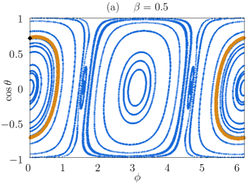
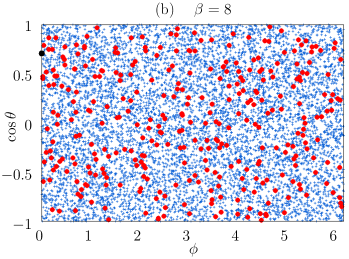
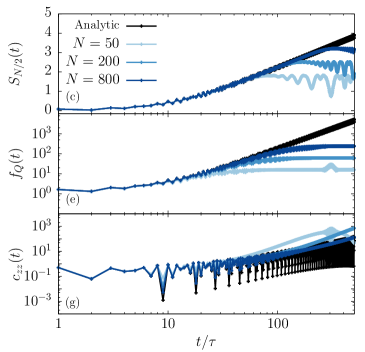
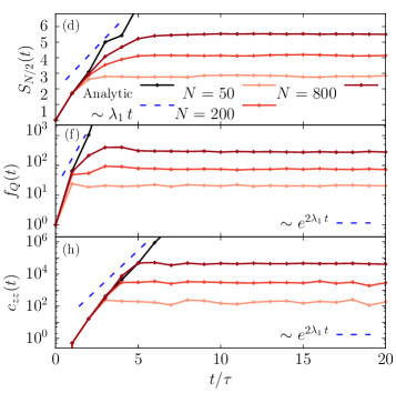
Figure 2: Dynamics of the quantum kicked top with $\alpha=\pi/2$, in the predominantly ordered and chaotic regimes with $\beta=0.5$ and $8$, respectively. Top panels: Poincarè map (stroboscopic phase-space trajectory) for the regular and chaotic dynamics, on the left (a) and right (b) panels, respectively. The black diamond and dot represent the initial condition of the orange (full line) and red (dotted) trajectory, respectively. This initial condition ($\phi_{0}=0$ and $\theta_{0}=\pi/4$) corresponds to the initial state for the quantum simulations in the bottom panels via Eq.(59). Bottom panels: We compare the corresponding analytical prediction [the black (upper) line] for the entanglement entropy (c,d), quantum Fisher information (e,f) and square commutator (g,h), valid in the thermodynamic limit, with exact computations at finite system size $N=50,\,200,\,800$. Here $\lambda_{1}=1.12$ is the maximal Lyapunov exponent computed in the Appendix C.3

.

VI.2 Numerical simulations

We compare the predictions of the semiclassical dynamics with the entanglement and chaos indicators obtained via exact numerical computations, specifically via exact diagonalization (ED).

Our general scheme is the following. We start from an initially polarized state on the Bloch sphere, which corresponds to a spin-coherent state parametrized by the two spherical angles angles $(\theta_{0},\phi_{0})$ as

$$\left|\psi_{0}\right\rangle=\left|\theta_{0},\phi_{0}\right\rangle=e^{i\phi_{0}\hat{S}_{z}}\,e^{i\theta_{0}\hat{S}_{y}}\,\left|S,S\right\rangle\ ,$$ (59)

where $\mathbf{\hat{S}}$ are the collective spin operators in Eq.(6) and $\left|S,S\right\rangle=\left|S=N/2,S_{z}=N/2\right\rangle$ is the fully polarized state in the $z$ direction.

Then, we let it evolve with the Floquet operator (12) generated by the Hamiltonian (11), and we compute the stroboscopic time-evolution of the entanglement entropy (19), the QFI (22) and the square commutator (24), at times $t_{n}=n\tau=0,1,2,\dots$ (recall that we have fixed $\tau=1$). In all our simulations, we fix $\alpha=\pi/2$, while $\beta$ ranges in a sufficiently large interval to appreciate the order/chaos transition in the classical limit.
Let us provide a few details on the ED simulations. We construct the initial state in Eq.(59) following Ref.Loh and Kim (2015) and compute the entanglement entropy using the decomposition in Ref.Latorre et al. (2005). The numerical QFI is given by the maximal eigenvalue of the covariance matrix ${\text{Cov}(\hat{A},\hat{B})=4\langle\hat{A}\hat{B}\rangle-4\langle\hat{A}\rangle\langle\hat{B}\rangle}$ with $\hat{A},\hat{B}=\hat{S}^{x,y,z}$ Gabbrielli et al. (2019). For the square commutator (24), we choose ${\hat{A}=\hat{B}=\hat{S}^{z}/S}$, for definiteness.

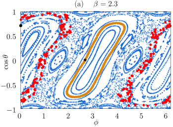
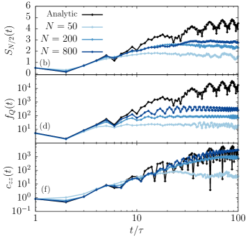
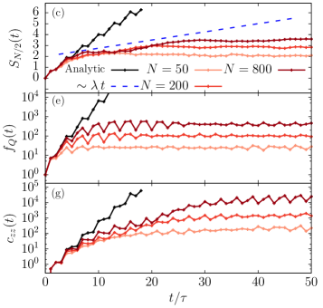
Figure 3: Dynamics of the quantum kicked top with $\alpha=\pi/2$, in the intermediate regime across the order/chaos transition, with $\beta=2.3$. Top panel (a): Poincarè map (stroboscopic phase-space trajectories). The black dot and diamond, giving rise to the red (dotted) and orange (full line) trajectories, indicate the initial condition of the simulations in the bottom panels. Bottom panels: Comparison between the analytical prediction [the black (upper) line] for the entanglement entropy (b,c), quantum Fisher information (d,e) and square commutator (f,g), valid in the thermodynamic limit, and exact computations at finite $N=50,\,200,\,800$. Left panels: Initial condition $\theta_{0}=\pi/4$, $\phi_{0}=0$ corresponding to a regular trajectory. Right panels: Initial condition $\theta_{0}=\pi/4$, $\phi_{0}=2.7$ corresponding to a chaotic trajectory. Here $\lambda_{1}=0.08$ is the maximal Lyapunov exponent computed in the Appendix C.3.

For the semiclassical analysis, we apply the discrete-time map in Eqs.(13a-13b) for the classical phase space — the Bloch sphere, parameterized by the canonically conjugated variables $\cos\theta$ and $\phi$ as in Eqs.(13) — and in Eqs.(58) for the quantum fluctuations. The initial conditions are $(\,\cos\theta(0),\phi(0),G_{qq}(0),G_{pp}(0),G_{qp}(0)\,)=(\cos\theta_{0},\phi_{0},1/2,1/2,0)$, which represent the state in Eq.(59). From the time evolution, we directly compute the entanglement entropy, QFI and $c_{zz}(t)$ from Eqs.(46-47), Eq.(49) and Eq.(52), respectively.

A remark is in order concerning the semiclassical numerical methods. For these kinds of simulations, it is crucial that the numerical integration is symplectic. For single degrees of freedom, simplecticity reduces to the conservation of the volume in phase space, i.e., $\det G(t)\equiv 1/4$. Although the map in Eqs.(58) is exact, we find violations of this conservation law after a few kicks in the chaotic regime, due to machine-precision errors. To the aim of presenting accurate results for the time windows shown in the figures below, we have resorted to a multi-precision arithmetic library Johansson et al. (2013a) and fixed the precision to at least $400$ digits.

VI.3 Discussion

We study, as a function of the kicking strength $\beta$, how the qualitative change in the semi-classical phase space across the order/chaos transition determines a change in the dynamics of the entanglement.

In Fig.2 we present the numerical results deep in the two orderly and chaotic phases. For small $\beta$ (left panels), the phase-space trajectories are mostly regular KAM tori. In this case, the classical Lyapunov exponent is vanishing. Accordingly, the asymptotic growth of quantum fluctuations in the semiclassical regime is polynomial in time. The theory in Sec.V predicts a logarithmic growth of the bipartite entanglement entropy and an exponential growth of the quantum Fisher information and of the square commutator. As shown in panels (c,e,g), the ED numerical data follow the semiclassical curves for a time window $T_{\text{Eh}}(N)\thicksim\sqrt{N}$ that increases with the system size.
Conversely, for large $\beta$ (right panels), chaos is fully developed in the classical phase space, and the motion is practically ergodic. The Lyapunov exponent $\lambda$ is thus positive and almost uniform. The theory in Sec. V predicts a linear growth of the bipartite entanglement entropy, with an asymptotic average slope $\lambda$, and an exponential growth of the quantum Fisher information and of the square commutator, with an asymptotic average rate $2\lambda$. As shown in panels (d,f,h), the ED numerical data follow the semiclassical curves for a time window $T_{\text{Eh}}(N)\thicksim\ln{N}$ that increases slowly with the system size.
Hence, we turn to the intriguing intermediate regime across the order/chaos transition, characterized by a complex structure of phase-space trajectories featuring persisting KAM tori forming stability islands in a growing chaotic sea (we adopt here the standard figurative terminology in the literature). It is widely known that the point-to-point and finite-time fluctuations of the Lyapunov spectrum are typically strong in Hamiltonian systems with a mixed phase space. The comparison in Fig. 3 allow us to test the theory of Sec. V. Even in this case, the finite-size numerical data of the quantum evolution approach the result of the semiclassical computation as $N\to\infty$ for an increasing time window. The behavior of the entanglement and chaos indicators for both the sample regular and chaotic initial states are partially masked by enhanced oscillations as compared to the corresponding evolution in Fig. 6. Despite this effect, the distinction between the two qualitative behaviors is apparent.
In all cases, we observe some extent of discrepancy between the slope or rate of the transient growth of our indicators, and those compatible with the asymptotic Lyapunov exponent. This discrepancy is typically more pronounced when the phase space is complex and mixed [cf. Fig. 3] than in a fully chaotic phase space [cf. Fig. 2]. In Appendix C.3 we show that this is reflected in the rate of convergence of the numerical computations of $\lambda$.

VII The Dicke model

In this section, we will apply the theoretical analysis of Sec.V to the Dicke model introduced in Sec.III.6. We will first derive the semiclassical evolution of the quantum fluctuations in Sec.V.1. Then, in Sec.VII.2 we compare our analytical predictions with exact numerics in finite-size systems only for the entanglement entropy dynamics. Note that the QFI and the square commutator have been explored in the same context recently Song et al. (2012); Wang et al. (2014); Zhang and Chen (2015); Mirkhalaf and Smerzi (2017); Gietka et al. (2019); Bhattacherjee and Sharma (2016); Buijsman et al. (2017); Alavirad and Lavasani (2019); Chávez-Carlos et al. (2019); Lewis-Swan et al. (2019).

VII.1 Evolution of the quantum fluctuations

The evolution of the quantum fluctuations around the classical coupled evolution of the collective spin and of the cavity mode (17) can be obtained by adapting the method of Secs.V.1 and V.2. The collective spin fluctuations may be described via a Holstein-Primakoff expansion around the time-dependent direction of the average spin orientation ${\vec{\mathcal{S}}(t)\equiv\big{\langle}\hat{\mathbf{S}}(t)\big{\rangle}\propto{\mathbf{Z}}}$, i.e. Eq.(35). The cavity-mode fluctuations are represented by deviations away from its macroscopic expectation value (16)

$$\left\{\begin{split}\hat{Q}&=\sqrt{N}\mathcal{Q}(t)+\delta\hat{Q}\ ,\\ \hat{P}&=\sqrt{N}\mathcal{P}(t)+\delta\hat{P}\ .\end{split}\right.$$ (60)

The quantum fluctuations are thus compactly denoted by ${\delta\hat{\bm{\xi}}=(\delta\hat{Q},\delta\hat{P},\delta\hat{q},\delta\hat{p})}$. As explained in Sec.III.6, the $\sqrt{N}$ scaling of classical variables may be understood as the occurrence that all terms in the Hamiltonian are extensive and balance each other in equilibrium. Conversely, typical quantum fluctuations in equilibrium, quantified by the expectation values of quadratic bosonic operators, are of order $\mathcal{O}(1)$, i.e., subextensive. This corresponds to having an effective Planck’s constant $\hbar_{\text{eff}}=1/N$.

The semiclassical equations of motion are found by applying the method of Sec.V.1. Substituting the expansions in Eqs. (35) and (60) into the Dicke Hamiltonian (14) and truncating it at the quadratic order, one finds the same structure as in Eq. (38). The classical trajectory $\mathcal{Q}(t),\mathcal{P}(t)$ and $\mathbf{Z}(t)$ is determined by the vanishing of the linear term in the quantum fluctuations, i.e., $\hat{H}_{1}(t)\equiv 0$. Their dynamics are thus regulated by the quadratic Hamiltonian $\hat{H}_{2}(t)$, from which we find Eq.(39), i.e.

$$\frac{d\,}{dt}\delta\hat{\bm{\xi}}=A(t)\,\delta\hat{\bm{\xi}}\ ,$$ (61)

with

$$A(t)=\begin{pmatrix}0&\omega&0&0\\ -\omega&0&-\frac{\gamma}{\sqrt{2}}\cos\theta\cos\phi&\frac{\gamma}{\sqrt{2}}\,\sin\phi\\ -\frac{\gamma}{\sqrt{2}}\sin\phi&0&0&-\gamma\mathcal{Q}\frac{\cos\phi}{\sin\theta}\\ -\frac{\gamma}{\sqrt{2}}\,\cos\theta\cos\phi&0&+\gamma\mathcal{Q}\frac{\cos\phi}{\sin\theta}&0\end{pmatrix}\ .$$ (62)

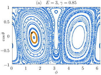
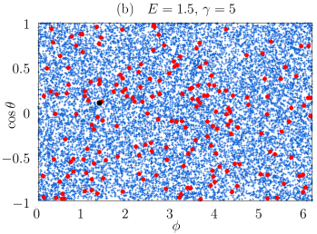
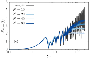
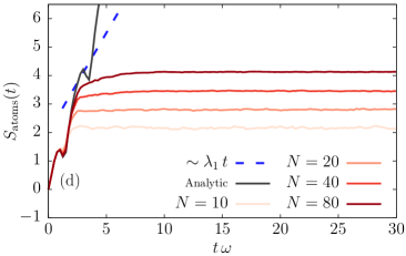
Figure 4: Entanglement dynamics for the Dicke model in the regular (a) and chaotic (b) regime with $E=3$, $\gamma=0.85$ and $E=1.5$, $\gamma=5$. (a-b) Poincarè maps with $\mathcal{P}=0$ and $\mathcal{Q}>0$ at fixed energies. The black diamond and dot correspond to the initial condition $(Q_{0},P_{0},\theta_{0},\phi_{0})$ $=(Q(E,\theta_{0},\phi_{0}),\,0.,\,\theta_{0},\phi_{0})$ with $\theta_{0}=\text{arcos}(0.1)$ and $\phi_{0}=1.4$ chosen for the simulation of the entanglement entropy below. (c-d) Comparison between the semi-classical result [the black (upper) line] with exact ED computations at finite $N=10,\,20,\,40,\,80$. (c) Dynamics in regular phase-space $E=3$, $\gamma=0.85$. (d) Dynamics in chaotic phase-space $E=1.5$, $\gamma=5$. Here $\lambda_{1}=0.7$ is the maximal Lyapunov exponent computed in the Appendix C.3.

Hence, the evolution of the correlation matrix $G(t)$ is determined via Eq.(42) from $A(t)$ by integrating Eq.(61). The details of the calculation to obtain Eq.(62) are reported in Appendix B.2. Together with Eqs.(17) and with the appropriate initial conditions, Eqs.(61,62) give a complete description of the semiclassical dynamics of the Dicke model, before the Ehrenfest time scale $T_{\text{Eh}}$.

VII.2 Numerical simulations

We now compare the semiclassical predictions for entanglement and chaos indicators with the numerical results obtained via exact diagonalization (ED) of the Hamiltonian.

We start from an initial state, which is a tensor product of a spin coherent state of the atomic ensemble and a bosonic coherent state for the cavity, namely

$$\left|\Phi_{0}\right\rangle=\left|\theta_{0},\phi_{0}\right\rangle\otimes\left|\alpha\right\rangle\quad\text{with}\quad\alpha=\frac{\mathcal{Q}_{0}+i\mathcal{P}_{0}}{\sqrt{2}}\ ,$$ (63)

where $\left|\theta_{0},\phi_{0}\right\rangle$ is the spin coherent state defined in Eq.(59), while the bosonic coherent state $\left|\alpha\right\rangle=e^{i(\alpha\hat{b}^{\dagger}+\alpha^{*}\hat{b})}\left|0\right\rangle$ is obtained by displacing the standard bosonic coherent vacuum $\left|0\right\rangle$ (defined by $\hat{b}\left|0\right\rangle=0$, $\braket{0}{0}=1$) by the complex vector $\alpha$. This quantum initial state corresponds to a minimal-uncertainty Gaussian distribution in the classical phase space, centered around the point $(\mathcal{Q}_{0},\mathcal{P}_{0},\cos\theta_{0},\phi_{0})$ (see e.g. Refs.de Aguiar et al. (1992); Furuya et al. (1998)). Then, we let evolve the system with the Dicke Hamiltonian (14) and we study the temporal development of quantum correlations.

We perform exact diagonalization using QuTip, an open-source software for quantum optics dynamics Johansson et al. (2012, 2013b). The spin Hilbert space is treated exactly, while we set a large cutoff $N_{\text{cut}}$ on the photon Hilbert space, checking that the results are converged upon increasing $N_{\text{cut}}$. In all simulations, we take a maximum ${N_{\text{cut}}=\Delta\times N}$, where $N$ is the number of spins and $\Delta\thicksim 4\div 8$ varies depending on the trajectory. A convenient way to a priori estimate the needed magnitude of $\Delta$ is to evaluate the maximum of $(\mathcal{Q}^{2}(t)+\mathcal{P}(t)^{2})/2$ along the reference classical trajectory in the target time window.

In the semiclassical simulations, we start from the classical initial conditions corresponding to the quantum state (63). We fix $\mathcal{P}_{0}=0$ and the value of the energy $E$. The classical initial condition is then $(\mathcal{Q}_{0}(E,\phi_{0},\theta_{0}),0,\cos\theta_{0},\phi_{0})$.

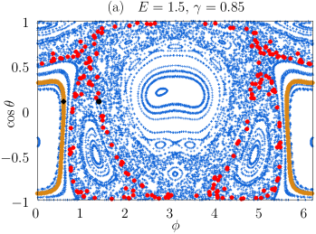
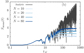
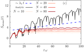
Figure 5: Entanglement dynamics for the Dicke model in the mixed regime with $E=1.5$ and $\gamma=0.85$. (a) Poincarè map with $\mathcal{P}=0$ and $\mathcal{Q}>0$ at fixed energy $E=1.5$ with $\gamma=0.85$. The black diamond (dot) correspond to regular (chaotic) initial conditions $(Q_{0},P_{0},\theta_{0},\phi_{0})$ $=(Q(E,\theta_{0},\phi_{0}),\,0.,\,\theta_{0},\phi_{0})$ with $\theta_{0}=\text{arcos}(0.1)$ and $\phi_{0}=0.6$ ($\phi_{0}=1.4$). (b-c) Comparison between the semi-classical entanglement entropy [the black (upper) line] with exact ED computations at finite $N=10,\,20,\,40,\,80$. (b) Dynamics starting from the regular initial condition $\phi_{0}=0.6$ (diamond in (a)). (c) Dynamics starting from the chaotic initial condition $\phi_{0}=1.4$ (dot in (a)). Here $\lambda_{1}=0.03$ is the maximal Lyapunov exponent computed in the Appendix C.3.

We then numerically integrate Eqs.(17),(61). Since the Dicke Hamiltonian (14) is non-separable — i.e., it cannot be decomposed as $\mathcal{H}(\mathbf{q},\mathbf{p})=K(\mathbf{p})+V(\mathbf{q})$ — efficient symplectic integrators are not available. For this reason, we employ an auto-adaptive fourth-order Runge-Kutta algorithm, fixing the relative and absolute accuracy to $10^{-14}$. The lack of symplecticity of the numerical integration is witnessed, e.g., by violations of the phase-space volume conservation. This limitations restricts the validity of the classical simulations to relatively short times in the chaotic regimes.

Time-evolution is visualized via Poincaré sections at fixed energy $E=H(\mathcal{Q}_{0},0,\cos\theta_{0},\phi_{0})$ and $\mathcal{P}=0$ in the four-dimensional phase space: the diagrams trace out the sequence of points in the $\cos\theta-\phi$ plane where the trajectory pierces the Poincaré section with $\mathcal{Q}>0$. The natural entanglement bipartition in the Dicke model consists in subdividing the degrees of freedom of the atoms and the cavity mode. For any initial state (63), the semiclassical entanglement entropy is thus computed from Eq.(46).

VII.3 Discussion

Similarly to the analysis of the quantum kicked top, we investigate all the qualitative dynamical regimes of the Dicke model and validate the correspondence between the entanglement dynamics and chaoticity properties in the semiclassical regime. Unlike the quantum kicked top, the Dicke model represents an isolated (undriven) system, so the energy is conserved. As its value of $E$ and/or of the coupling $\gamma$ are varied, the accessible phase space may undergo a progressive order/chaos transition Emary and Brandes (2003). This allows us to test the theoretical conclusions of Sec.V for autonomous dynamics.

In Fig.4, we show the Poincaré sections in two limiting cases of predominantly regular and chaotic behavior, in the top left and right panels, respectively. The initial state in Eq.(63) associated with the classical phase-space point denoted by a black marker is selected and the corresponding time-evolution of the von Neumann entanglement entropy between atoms and cavity mode is shown in the bottom panels. As it is apparent, the relation between orderly collective motion and slow logarithmic growth of entanglement on one side, and between collective chaos and fast linear growth of entanglement on the other side, is strongly corroborated by the outcome of the simulations.

In Fig.5 we turn to the intermediate regime of mixed classical phase-space across the order/chaos transition. The system is prepared in the two initial states corresponding to the phase-space points marked in black in the Poincaré section (top panel), representative of regular and chaotic trajectories, and the relative nonequilibrium dynamics of the entanglement entropy between atoms and cavity is displayed in the bottom panels. Similarly to the case of the quantum kicked top, the asymptotic growth of the entanglement entropy is partly obscured by pronounced oscillations and strong finite-time fluctuations. However, convergence to the semiclassical prediction upon increasing the number $N$ of atoms is observed over an increasing time window.

As in the case of quantum kicked top, we observe deviations between the slope or rate of the transient growth of the entanglement entropy, and that compatible with the asymptotic Lyapunov spectrum. Even in this case, this effect tends to be more pronounced when the phase space is complex and mixed [cf. Fig.5] than in a fully chaotic phase space [cf. Fig.4]. Appendix C.3 discusses the rate of convergence of the numerical computations of the Lyapunov spectrum, highlighting the connection with the discrepancies presented in Figs.4 and 5.

VIII Conclusions and perspectives

In this work, we presented a unifying framework underlying the growth of entanglement in systems characterized by a well-defined classical limit, in agreement with previous suggestions in the literature Zurek and Paz (1994); Bianchi et al. (2018); Lewis-Swan et al. (2019). Overall, the established picture that the transient entanglement growth happens via decoherence was confirmed, and the exact relationship between the notions of bipartite entanglement, multipartite entanglement and scrambling was clarified in the semiclassical regime. Quantum entanglement indicators approach a finite limit as the effective Planck’s constant vanishes, $\hbar_{\text{eff}}\to 0$ Zurek and Paz (1995); Casati et al. (2012), and this limit possesses a clean interpretation in terms of the subsystem quantum fluctuations around the classical trajectory. Their temporal growth is associated with the chaoticity properties of the underlying classical phase space. This allows to make clear quantitative predictions on the asymptotic entanglement growth, based on the knowledge of the classical limit: Before the Ehrenfest time, for regular dynamics the entanglement entropy $S_{A}(t)$ grows only logarithmically in time, while the QFI and the square commutator polynomially; for chaotic dynamics, $S_{A}(t)$ undergoes a linear growth with a coefficient given by the classical Kolmogorov-Sinai entropy rate, while the QFI and the square commutator grow exponentially with a rate set by twice the largest classical Lyapunov exponent. This discussion is summarized in Table 1. For the entanglement entropy dynamics, this classification builds on the results of Ref. Bianchi et al. (2018); Hackl et al. (2018) for quadratic bosonic Hamiltonians. To the best of our knowledge, these results constitute the first general prediction for the dynamics of the quantum Fisher information and collective spin-squeezing in the semiclassical limit. We further discussed the finite-time fluctuations of entanglement quantifiers, crucial in finite quantum systems with a relatively short saturation time, and relate them to the underlying classical trajectories. We finally corroborated our analysis via detailed numerical computations in paradigmatic many-body collective quantum systems of current experimental relevance which undergo an order/chaos transition, namely the quantum kicked top and the Dicke model, finding excellent agreement with the analytical predictions in all dynamical regimes.

The semiclassical analysis presented here underlies the slow growth of entanglement in spin systems with algebraically-decaying interactions Lerose and Pappalardi (2020). The same approach could be applied to the entanglement growth in open systems, where it has been already shown that quantum fluctuations around the mean-field observables are the responsible for the growth of the entanglement negativity Benatti et al. (2017).

A very challenging problem is to understand how quantum interference effects enter the game after the Ehrenfest time, causing a saturation of the entanglement quantifiers Rammensee et al. (2018). In fact, the intriguing occurrence that the long-time average of entanglement quantifiers bears signatures of the underlying classical phase space even for intermediate $\hbar_{\text{eff}}$ is still incompletely understood and is a matter of ongoing debate Bhosale and Santhanam (2018); Ruebeck et al. (2017).

It is worth stressing that our results contribute to establish a clear predictive framework for the study of entanglement dynamics in more general semiclassical approaches, such as those based on time-dependent variational principles Hallam et al. (2019); Michailidis et al. (2020); Ho et al. (2019). Also, they can likely be extended to match complementary approaches to entanglement dynamics such as that in Ref. Kumari and Ghose (2019).

We finally reiterate that the connection between entanglement dynamics and chaos studied here, has direct experimental relevance for the detection of entanglement and its dynamics via measurements of collective quantities Ghose et al. (2008); Bohnet et al. (2016); Gärttner et al. (2017), the experimental accessibility of which is well-established with standard techniques and tools of quantum atomic experiments — see Fig.1 and the relative discussion.

Appendix A
Dynamics in fully connected models:
Mapping to an effective classical dynamics

In this appendix, we review the general mapping, due to Sciolla and Biroli Sciolla and Biroli (2011), of the quantum dynamics of permutationally-symmetric systems onto the effective semiclassical dynamics of their collective variables in the thermodynamic limit.

With reference to the setting and notations of Sec.III.1, one observes that possible off-diagonal transitions governed by the permutationally-symmetric Hamiltonian $\hat{H}$, are uniquely identified by a set of integers $m_{1},\dots,m_{q}$

$$\Ket{N_{1},\dots,N_{q}}\to\Ket{N_{1}+m_{1},\dots,N_{q}+m_{q}}.$$ (64)

For convenience, we turn the occupation numbers $N_{\alpha}$ into fractions $x_{\alpha}\equiv N_{\alpha}/N$, with $0\leq x_{\alpha}\leq 1$ and $\sum_{\alpha=1}^{q}x_{\alpha}=1$, and denote basis states by $\Ket{\mathbf{x}}$, where $\mathbf{x}=(x_{1},\dots,x_{q})$. Hence, we write the matrix elements of $\hat{H}$ as

$$H_{\mathbf{x},\mathbf{x}^{\prime}}\equiv\braket{\mathbf{x}}{\hat{H}}{\mathbf{x}^{\prime}}=V(\mathbf{x})\,\delta_{\mathbf{x},\mathbf{x}^{\prime}}-\sum_{\mathbf{m}\neq\mathbf{0}}T_{\mathbf{m}}(\mathbf{x})\delta_{\mathbf{x},\mathbf{x}^{\prime}+\mathbf{m}/N}\ ,$$ (65)

with $\mathbf{m}=(m_{1},\dots,m_{q})\in\mathbb{Z}^{q}$. Terms in the Hamiltonian $\hat{H}$ involving up to $k$ bodies yield “local” transitions in the TSS basis, characterized by $\lvert\mathbf{m}\rvert\equiv\sum_{\alpha}\lvert m_{\alpha}\rvert\leq 2k$. By the extensivity of the Hamiltonian $\hat{H}$, both $V(\mathbf{x})$ and $T_{\mathbf{m}}(\mathbf{x})$ are extensive,

$$V(\mathbf{x})\thicksim N\,v(\mathbf{x}),\qquad T_{\mathbf{m}}(\mathbf{x})\thicksim N\,t_{\mathbf{m}}(\mathbf{x})\ .$$ (66)

Crucially, the densities $v$ and $t$ are smooth functions of $\mathbf{x}$, as they generally result from combinatoric factors of the occupation numbers which are insensitive to small changes $N_{\alpha}\mapsto N_{\alpha}\pm 1,2,\dots$ to the leading order in the thermodynamic limit $N\to\infty$ Sciolla and Biroli (2011). These properties allow one to rewrite the Schrœdinger equation for the TSS wavefunction $\psi(\mathbf{x},t)$ as

$$\frac{i}{N}\frac{\partial}{\partial t}\psi(\mathbf{x},t)=\bigg{\{}v(\mathbf{x})-\sum_{{\mathbf{m}}}t_{\mathbf{m}}(\mathbf{x})\cosh\bigg{(}\frac{\mathbf{m}}{N}\cdot\frac{\partial}{\partial\mathbf{x}}\bigg{)}\bigg{\}}\psi(\mathbf{x},t)\ .$$ (67)

Defining the operators

$$x_{\alpha}\mapsto\hat{q}_{\alpha},\qquad-i\hbar_{\text{eff}}\frac{\partial}{\partial x_{\alpha}}\mapsto\hat{p}_{\alpha}\ ,$$ (68)

one recognizes that the evolution in Eq. (67) is governed by the effective Hamiltonian

$$\mathcal{H}_{\text{cl}}(\hat{\mathbf{q}},\hat{\mathbf{p}})\equiv v(\hat{\mathbf{q}})-\sum_{\mathbf{m}}t_{\mathbf{m}}(\hat{\mathbf{q}})\cos(\mathbf{m}\cdot\hat{\mathbf{p}})\ ,$$ (69)

with an effective Planck’s constant

$$\hbar_{\text{eff}}\equiv\frac{1}{N}\qquad\text{($\hbar=1$ in our units)}$$ (70)

that approaches zero in the thermodynamic limit. Thus, the dynamics of the original system of all-to-all interacting $q$-level units is equivalent to the semiclassical dynamics of $q-1$ collective degrees of freedom via Eq. (69) (due to the constraint $\sum_{\alpha}^{q}x_{\alpha}\equiv 1$).

Appendix B
Derivation of the semiclassical evolution equations

In this appendix we derive the equations of motion of the classical collective variables and of the quantum fluctuations, for the quantum kicked top and the Dicke model.

B.1 Kicked top

We start by deriving the stroboscopic map for the classical limit of the kicked top, cf. Eq. (13). With reference to the setting and notations of Sec.III.5, we adopt a convenient parametrization of the spin via spherical coordinates along the $z$ axis via (9), so that the nonlinear part of the evolution — the kick $\hat{U}_{\beta}$ — looks simple. The discrete classical map that describes the stroboscopic evolution of the collective spin on the Bloch sphere is the composition of two maps, respectively generated by $\hat{U}_{\alpha}$ and $\hat{U}_{\beta}$.

The classical map generated by $\hat{U}_{\beta}$ reads

$$\begin{dcases}\theta^{\prime\prime}=\theta^{\prime}\\ \phi^{\prime\prime}=\phi^{\prime}+\beta\cos\theta^{\prime}\end{dcases}\ .$$ (71)

Due to the our choice of coordinates, obtaining the free precession described by $\hat{U}_{\alpha}$ is less straightforward. One strategy is to work it out in spherical coordinates with polar axis along $x$, and to transform into the original coordinates before and after the application of $\hat{U}_{\alpha}$. To this aim, we reparameterize the time-dependent collective spin direction as

$${\mathbf{Z}}=\begin{pmatrix}\cos\eta\\ \sin\eta\cos\xi\\ \sin\eta\sin\xi\end{pmatrix}\ ,$$ (72)

where $\eta$ and $\xi$ are respectively the polar and azimuthal angle in spherical coordinates with respect to the $x$ axis. With this choice, the classical precession is described as

$$\begin{dcases}\eta^{\prime}=\eta\\ \xi^{\prime}=\xi+\alpha\end{dcases}\ .$$ (73)

The expression in the original coordinates is obtained by mapping $(\eta,\xi)$ one-to-one to $(\theta,\phi)$ by equating the two expressions of $\mathbf{Z}$ in Eqs. (9) and (72). This transformation yields Eqs.(13).

Let us now determine the evolution of the quantum fluctuations. The transformation generated by $\hat{U}_{\beta}$ can be obtained straightforwardly following the procedure described in Sec.V.1. One gets $\widetilde{H}_{2}=\frac{1}{2}\beta\sin^{2}\theta\;\delta\hat{q}^{2}$ in Eq. (38), and hence

$$\begin{dcases}\delta\hat{q}^{\prime\prime}=\delta\hat{q}^{\prime}\\ \delta\hat{p}^{\prime\prime}=\delta\hat{p}^{\prime}-\beta\,\sin^{2}\theta^{\prime}\,\delta\hat{q}^{\prime}\end{dcases}\ .$$ (74)

To obtain the discrete transformation generated by $\hat{U}_{\alpha}$, we can again resort to the adapted coordinates $(\eta,\xi)$. We define the rotated frame $(\bar{{\mathbf{X}}},\bar{{\mathbf{Y}}},\mathbf{Z})$ with the new spherical angles $\theta\to\eta$, $\phi\to\xi$, i.e.,

$$\bar{{\mathbf{X}}}\equiv\partial_{\eta}{\mathbf{Z}}/{\lvert\partial_{\eta}{\mathbf{Z}}\rvert}\ ,\qquad\bar{{\mathbf{Y}}}\equiv\partial_{\xi}{\mathbf{Z}}/{\lvert\partial_{\xi}{\mathbf{Z}}\rvert}\ ,$$ (75)

such that $(\bar{{\mathbf{X}}},\bar{{\mathbf{Y}}},{{\mathbf{Z}}})$ is an orthonormal frame adapted to the $(\eta,\xi)$-parametrization of the sphere. Along these lines, we define the corresponding transverse spin components and the associated bosonic variables via the truncated Holstein-Primakoff transformation,

$$\hat{S}^{\bar{X}}\equiv\bar{{\mathbf{X}}}\cdot\hat{\mathbf{S}}\simeq\sqrt{Ns}\,\delta\bar{q}\ ,\qquad\hat{S}^{\bar{Y}}\equiv\bar{{\mathbf{Y}}}\cdot\hat{\mathbf{S}}\simeq\sqrt{Ns}\,\delta\bar{p}\ .$$ (76)

In this description, the free precession around $x$ generated by $\hat{U}_{\alpha}$ is exactly canceled by the inertial term, and one obtains

$$\begin{dcases}\delta\bar{q}^{\prime}=\delta\bar{q}\\ \delta\bar{p}^{\prime}=\delta\bar{p}\end{dcases}\ .$$ (77)

Now, we only need to find the relation between $(\delta\bar{q},\delta\bar{p})$ and $(\delta\hat{q},\delta\hat{q})$. This can be obtained by noting that both $(\bar{{\mathbf{X}}},\bar{{\mathbf{Y}}})$ and $({{\mathbf{X}}},{{\mathbf{Y}}})$ are orthonormal bases of the tangent plane to the unit sphere at the point ${{\mathbf{Z}}}$. Therefore, they must be related via a rotation, i.e.,

$$\begin{dcases}\bar{{\mathbf{X}}}&=+\cos\psi\,{{\mathbf{X}}}+\sin\psi\,{{\mathbf{Y}}},\\ \bar{{\mathbf{Y}}}&=-\sin\psi\,{{\mathbf{X}}}+\cos\psi\,{\mathbf{Y}}\end{dcases}\ .$$ (78)

for some angle $\psi\in[0,2\pi)$. This angle can be determined by noting that, by construction, $\bar{{\mathbf{X}}}$ belongs to the plane generated by ${\mathbf{x}}$ and ${\mathbf{Z}}$, and hence the equation

$$\bar{{\mathbf{X}}}\cdot({\mathbf{x}}\times{\mathbf{Z}})=0$$ (79)

holds. Substituting the first of Eqs. (78) as well as the third of Eqs. (9), we find

$$\psi=-\arctan\left(\frac{\tan\phi}{\cos\theta}\right)\ ,$$ (80)

which determines $\psi$ up to the ambiguity $\psi\leftrightarrow\psi+\pi$. Equation (78) immediately yields

$$\begin{dcases}\delta\bar{{q}}&=+\cos\psi\,\delta\hat{{q}}+\sin\psi\,\delta\hat{{p}},\\ \delta\bar{{p}}&=-\sin\psi\,\delta\hat{{q}}+\cos\psi\,\delta\hat{{p}},\\ \end{dcases}\ .$$ (81)

hence one finds

$$\begin{dcases}\delta\hat{q}^{\prime}=+\cos(\psi-\psi^{\prime})\,\delta\hat{q}+\sin(\psi-\psi^{\prime})\,\delta\hat{p}\\ \delta\hat{p}^{\prime}=-\sin(\psi-\psi^{\prime})\,\delta\hat{q}+\cos(\psi-\psi^{\prime})\,\delta\hat{p}\end{dcases}\ .$$ (82)

Substituting the two maps in Eqs. (74) and (82) into the definition (41) of the correlation matrix $G(t)$, one directly obtains the desired, ambiguity-free, discrete-time evolution equations (58) for the quantum fluctuations.

B.2 Dicke model

Here, we derive the equations for the classical trajectory (17) and for the evolution of the quantum fluctuations around it (62) generated by the Dicke Hamiltonian (14) for large $N$.

Collective spin fluctuations can be described via a Holstein-Primakoff expansion around the time-dependent direction of the average orientation, as discussed in Sec.V.2.1. Cavity mode fluctuations are represented by deviations away from its macroscopic expectation value. With reference to the setting and notations of Sec.III.6, one has:

$$\hat{S}^{\alpha}\simeq{X}_{\alpha}(t)\;\sqrt{\frac{N}{2}}\;\delta\hat{q}\;+{Y}_{\alpha}(t)\;\sqrt{\frac{N}{2}}\;\delta\hat{p}$$ (83)

$$\qquad\qquad\qquad\qquad+{Z}_{\alpha}(t)\;\left(\frac{N}{2}-\frac{\delta\hat{q}^{2}+\delta\hat{p}^{2}-1}{2}\right)$$

$$\hat{Q}=\sqrt{N}\mathcal{Q}(t)+\delta\hat{Q}$$ (84)

$$\hat{P}=\sqrt{N}\mathcal{P}(t)+\delta\hat{P}$$ (85)

with $\alpha=x,y,z$. The classical functions $\mathcal{Q}(t)$, $\mathcal{P}(t)$ and $\mathbf{Z}(t)$ are chosen in such a way that they account for the classical dynamics of the system. As a consequence, the quantum bosonic operators $(\delta\hat{q},\delta\hat{p})$ and $(\delta\hat{Q},\delta\hat{P})$ have vanishing expectation values and describe quantum fluctuations around the classical dynamics. The $\sqrt{N}$ scaling of classical variables may be understood as the occurrence that all terms in the Hamiltonian are extensive (and balance each other in equilibrium). Conversely, typical quantum fluctuations in equilibrium, quantified by the expectation values of quadratic bosonic operators, are of order $\mathcal{O}(1)$, i.e., subextensive. This corresponds to having an effective Planck’s constant $\hbar_{\text{eff}}=\hbar/N$.

The semiclassical time-evolution of the system can be obtained by substituting the time-dependent expansion above into the Hamiltonian and truncating to quadratic order, cf. Eq.(38). We obtain

$$\hat{H}=\;N\,\mathcal{H}_{\text{cl}}\;+\sqrt{N}\,\hat{H}_{1}\;+\,\hat{H}_{2}\;+\,\mathcal{O}\bigg{(}\frac{1}{\sqrt{N}}\bigg{)}\ ,$$ (86)

with $\mathcal{H}_{\text{cl}}$ given by Eq.(15),

$$\begin{split}\hat{H}_{1}=&\sqrt{s}\big{(}\omega_{0}\,{X}_{z}+\gamma\mathcal{Q}\,{X}_{x}\big{)}\;\delta\hat{q}\\ &+\sqrt{s}\big{(}\omega_{0}\,{Y}_{z}+\gamma\mathcal{Q}\,{Y}_{x}\big{)}\;\delta\hat{p}\\ &+\big{(}\omega\mathcal{Q}+s\gamma\,{Z}_{x}\big{)}\;\delta\hat{Q}\;\;+(\omega\,\mathcal{P})\;\delta\hat{P}\end{split}$$ (87)

and

$$\begin{split}\hat{H}_{2}=&-\big{(}\omega_{0}\,{Z}_{x}+\gamma\mathcal{Q}\,{Z}_{x}\big{)}\frac{\delta\hat{q}^{2}+\delta\hat{p}^{2}-1}{2}\\ &\quad+\omega\frac{\delta\hat{Q}^{2}+\delta\hat{P}^{2}-1}{2}\\ &\quad+\sqrt{s}\gamma\Big{(}{X}_{x}\;\delta\hat{q}\,\delta\hat{Q}+{Y}_{x}\;\delta\hat{p}\,\delta\hat{Q}\Big{)}\ .\end{split}$$ (88)

The dynamics of quantum fluctuations are generated by the modified Hamiltonian $\widetilde{H}=\hat{H}-i\dot{\hat{V}}(t)\hat{V}^{\dagger}(t)$, which includes the inertial terms, due to the time-dependence of the transformation:

$$\begin{split}&\widetilde{H}_{1}=\;\hat{H}_{1}-\Big{(}\sqrt{s}\;\dot{\mathbf{Y}}\cdot\mathbf{Z}\;\delta\hat{q}+\sqrt{s}\;\dot{\mathbf{Z}}\cdot\mathbf{X}\;\delta\hat{p}-\dot{\mathcal{P}}\;\delta\hat{Q}+\dot{\mathcal{Q}}\;\delta\hat{P}\Big{)}\\ &\widetilde{H}_{2}=\;\hat{H}_{2}+\dot{\mathbf{X}}\cdot\mathbf{Y}\,\frac{\delta\hat{q}^{2}+\delta\hat{p}^{2}-1}{2}\ .\end{split}$$ (89)

In order for the quadratic approximation to be self-consistent, one must appropriately choose the classical functions $\mathcal{Q}(t)$, $\mathcal{P}(t)$ and $\mathbf{Z}(t)$ in such a way that linear terms in the bosonic variables vanish, i.e., $\widetilde{H}_{1}\equiv 0$. This results in the classical dynamics of the collective spin and the radiation field:

$$\begin{dcases}\dot{\mathcal{Q}}=\omega\mathcal{P}\\ \dot{\mathcal{P}}=-\omega\mathcal{Q}-\frac{\gamma}{2}{Z}_{x}\\ \dot{\mathbf{Y}}\cdot\mathbf{Z}=\omega_{0}\,{X}_{z}+\gamma\mathcal{Q}\,{X}_{x}\\ \dot{\mathbf{Z}}\cdot\mathbf{X}=\omega_{0}\,{Y}_{z}+\gamma\mathcal{Q}\,{Y}_{x}\end{dcases}\ .$$ (90)

The dynamics of quantum fluctuations is regulated by the equations of motion generated by the quadratic Hamiltonian $\widetilde{H}_{2}$ :

$$\begin{dcases}\dot{\delta\hat{Q}}=+\omega\delta\hat{P}\\ \dot{\delta\hat{P}}=-\omega\delta\hat{Q}-\sqrt{s}\gamma({X}_{x}\,\delta\hat{q}+{Y}_{x}\,\delta\hat{p})\\ \delta\dot{\hat{q}}=-(\omega_{0}\,{Z}_{z}+\gamma\mathcal{Q}\,{Z}_{x}-\dot{\mathbf{X}}\cdot\mathbf{Y})\delta\hat{p}+\sqrt{s}\gamma\,{Y}_{x}\,\delta\hat{Q}\\ \delta\dot{\hat{p}}=+(\omega_{0}\,{Z}_{z}+\gamma\mathcal{Q}\,{Z}_{x}-\dot{\mathbf{X}}\cdot\mathbf{Y})\delta\hat{q}-\sqrt{s}\gamma\,{X}_{x}\,\delta\hat{Q}\\ \end{dcases}\ .$$ (91)

With the usual choice of parametrization of the rotating frame (9)-(36) one has

$$\dot{\mathbf{Y}}\cdot\mathbf{Z}=-\sin\theta\dot{\phi}\ ,\qquad\dot{\mathbf{Z}}\cdot\mathbf{X}=\dot{\theta}\ ,\qquad\dot{\mathbf{X}}\cdot\mathbf{Y}=\cos\theta\dot{\phi}\ .$$ (92)

From these equations, by substituting explicitly the coordinates (9)-(36), one gets the classical equations of motion in Eq.(17) in the main text, and, for the fluctuations ${\delta\hat{\bm{\xi}}=(\delta\hat{Q},\delta\hat{P},\delta\hat{q},\delta\hat{p})}$, Eq. (91) can be written as

$$\frac{d\,}{dt}\delta\hat{\bm{\xi}}=A(t)\,\delta\hat{\bm{\xi}}\ ,$$ (93)

with the $4\times 4$ matrix $A(t)$ expressed by Eq.(62) in the main text.

Appendix C
Lyapunov exponents:
Theory and numerical applications

In this appendix, we will first recall the main definitions and properties of the Lyapunov spectrum in Sec.C.1. Then, in Sec.C.2, we will review the standard algorithm of Benettin et al. 1980 Benettin et al. (1980b) for computing it numerically. We conclude in Sec.C.3, by showing the application of the algorithm to the quantum kicked top and the Dicke model.

C.1 The Lyapunov spectrum and the maximum Lyapunov exponent

We recall here some elementary but important properties of the Lyapunov spectrum concerning the $K$-dimensional ordiented volumes delimited by $K$ tangent vectors, i.e. $\text{Vol}_{K}(t)=\text{Vol}[\mathbf{w}^{(1)}(t),\mathbf{w}^{(2)}(t),\dots\mathbf{w}^{(K)}(t)]$. An important consequence of the Oseledets theorem states that the expansion/contraction rate of $\text{Vol}_{K}(t)$ is given by the sum of the first $K$ exponents as

$$\Lambda_{K}=\sum_{k=1}^{K}\lambda_{k}=\lim_{t\to\infty}\frac{1}{t}\,\ln\left[\frac{\text{Vol}_{K}(t)}{\text{Vol}_{K}(0)}\right]\ .$$ (94)

This corresponds to the total expansion rate of a (generic) $K$-dimensional sub-manifold corresponding a subsystem of $K\leq d$ degrees of freedom. In particular, $\Lambda_{d}$ is the total expansion rate of the flow, i.e., the average of $\text{div}\,\mathbf{f}(\mathbf{x}(t))$ along the trajectory, which vanishes in conservative systems. For time-independent (autonomous) systems, one has $\lambda_{k}=0$ for some $k$, because the direction of the trajectory is neither stretched nor shrunk. For Hamiltonian systems, which are the focus of this work, Lyapunov exponents come in conjugate pairs $\lambda_{k}=-\lambda_{2n-k}$ due to the symplectic nature of the phase space flow. In this case, Liouville-integrability of the dynamics is signalled by $\lambda_{k}\equiv 0$ for all $k$ and in the whole phase space. By contrast, generic Hamiltonian systems do not possess analytic integrals of motion beyond their energy, and their constant-energy surfaces may present a complex structure with invariant submanifolds (KAM tori) intertwined by chaotic regions. In these cases, the Lyapunov spectrum presents strong phase-space and temporal fluctuations.

C.2 Benettin et al. algorithm for computing the Lyapunov spectrum

The by now standard numerical algorithm for a robust computation of the Lyapunov spectrum has been proposed by Benettin, Galgani and Strelcyn in a series of papers around 1980, see Refs. Benettin et al. (1976, 1980a, 1980b). Its central idea is based the evolution of $K$ tangent vectors $(\mathbf{w}^{(1)},\dots\mathbf{w}^{(K)})$ and the use of Eq.(94) to compute the volumes $\text{Vol}_{K}(t)$ and the resulting Lyapunov exponents $\{\lambda_{k}\}_{k=1}^{K}$. In chaotic systems, numerical errors grow exponentially fast in time and infinitesimal displacements $\mathbf{w}^{(k)}(t)$ might result in computer overflows at large $t$. To solve these issues, the method relies on the periodic orthonormalization of the evolved tangent-space basis, after a suitable time interval $s$. (This allows one to disregard the numerical instability due to the use of non-symplectic integrators.) In Ref.Benettin et al. (1980b), the authors show that by choosing the Gram-Schmidt orthonormalization procedure, one can evaluate all the volumes $\{\text{Vol}_{k}\}_{k=1}^{K}$ at once.

Fixing initial condition $\mathbf{x}(0)=\mathbf{x}_{0}$, the procedure goes as follows. Choose $K$ independent tangent vectors at random at $t=0$, i.e. $\{\mathbf{w}^{(k)}_{0}\}_{k=1}^{K}$. Then, for $1\leq i\leq n$:

1. evolve the vectors $\{\mathbf{w}^{(k)}_{(i-1)s}\}$ for a time interval $s$ via Eq.(27) and initial conditions $\mathbf{x}_{(i-1)s}$; this yields $\{\mathbf{w}^{(k)}_{is}\}$;

2. apply Gram-Schmidt procedure

   $$\alpha^{(1)}_{i}=|\mathbf{w}^{(1)}_{is}|\ ,\quad\mathbf{w}^{\prime(1)}_{is}=\mathbf{w}^{(1)}_{is}/\alpha^{(1)}_{i}$$ (95)

   where $|\cdot|$ is the euclidean norm . For $2\leq k\leq K$

   $$\alpha_{i}^{(k)} =\left|\mathbf{w}^{(k)}_{is}-\sum_{l=1}^{k-1}(\mathbf{w}^{\prime(l)}_{is}\cdot\mathbf{w}^{(k)}_{is})\,\mathbf{w}^{\prime(l)}_{is}\right|\ ,$$ (96a)

   $$\mathbf{w}^{\prime(k)}_{is} =\frac{1}{\alpha_{i}^{(k)}}\,\left(\mathbf{w}^{(k)}_{is}-\sum_{l=1}^{k-1}(\mathbf{w}^{\prime(l)}_{is}\cdot\mathbf{w}^{(k)}_{is})\,\mathbf{w}^{\prime(l)}_{is}\right)\ ;$$ (96b)

3. re-initialize the vectors $\mathbf{w}^{(k)}_{is}=\mathbf{w}^{\prime(k)}_{is}$ for $1\leq k\leq K$.

From this, the finite-time Lyapunov spectrum $\{\lambda_{k}(\mathbf{x}_{0})\}$ is computed as

$$\lambda^{(n,s)}_{k}(\mathbf{x}_{0})=\frac{1}{ns}\,\sum_{i=1}^{n}\,\ln\alpha_{i}^{(k)}\ ,$$ (97)

for $k\leq 1\leq K$. Convergence as $n\to\infty$ yields the proper, asymptotic Lyapunov spectrum. Notice that $\lambda^{(n,s)}_{k}(\mathbf{x}_{0})$ should not depend on the time-interval $s$ and on the number of iterations $n$ independently, but rather via the product $r=s\,n$, i.e. $\lambda^{(r)}_{k}(\mathbf{x}_{0})$. As $r$ increases, $\lambda^{(r)}_{k}$ approaches a well defined limit, the $k$-th Lyapunov exponent $\lambda_{k}=\lim_{r\to\infty}\lambda_{k}^{(r)}$.

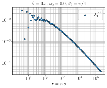
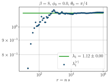
Figure 6: Convergence of the maximum Lyapunov exponent (97) for the kicked top dynamics in the predominantly regular and chaotic regimes. The trajectories shown here correspond to those in Fig.2, with initial condition $\phi_{0}=0$ and $\theta_{0}=\pi/4$: a regular one for $\beta=0.5$, with $s=2$ (top panel) and a chaotic one for $\beta=8$, with $s=10$ (bottom panel).

C.3 Lyapunov exponents for the kicked top and the Dicke model

We report the computation of the Lyapunov exponents of the kicked top (see Sec.VI.1) and of the Dicke model (see Sec.VII) obtained via the algorithm described in App.C.2.

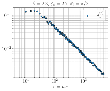
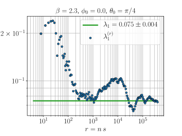
Figure 7: Convergence of the maximum Lyapunov exponent (97) for the kicked top dynamics in the intermediate regime with a mixed phase space. The trajectories correspond to those in Fig.3, with $\beta=2.3$: a regular one with $\theta_{0}=\pi/2$ and $\phi_{0}=2.7$ (top panel), and a chaotic one with $\theta_{0}=\pi/4$ and $\phi_{0}=0$ (bottom panel). Here we have fixed $s=5$.

We apply that procedure to the kicked top evolution at stroboscopic times (13), by evolving the linear displacements via the map in Eqs.(74-82). We fix a number $s$ of kicks and we study the black trajectories in Fig.2-3. The results are shown in Fig.6 and Fig.7 respectively. We plot the finite-time maximum Lyapunov exponent $\lambda_{1}^{(r)}$ in Eq.(97) as a function of $r$. The maximum Lyapunov exponent $\lambda_{1}$ (green in the plots) is extracted numerically by averaging over the last two decades of the time window. For regular initial conditions it approaches zero in the long-time limit $r\to\infty$, while for chaotic trajectories it clearly converges to a finite value, at very large times $r\gg 10^{4}$. As expected, the Lyapunov exponent for the chaotic trajectory in the intermediate regime with a mixed phase space is much smaller than the one for the fully chaotic phase, and convergence to the asymptotic value is much slower.

The same procedure is applied to the classical dynamics of the Dicke model (17), fixing $s=1$. The results for the regular and chaotic regimes are plotted in Fig.8 and for the intermediate regime with a mixed phase space in Fig.9. Because of the conservation of energy, the second Lyapunov exponent $\lambda_{2}$ always vanishes. As for $\lambda_{1}$, similar remarks to the case of the kicked top apply.

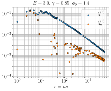
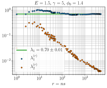
Figure 8: Convergence of the maximum Lyapunov exponent (97) for the Dicke model dynamics in the predominantly regular and chaotic regimes. Top panel: regular trajectory with $E=3$, $\gamma=0.85$ Bottom panel: chaotic trajectory with $\beta=1.5$, $\gamma=5$. The common initial condition $\phi_{0}=1.4$ and $\cos\theta_{0}=0.1$ corresponds to the two trajectories in Fig.4. Here we have set $s=0.5$.

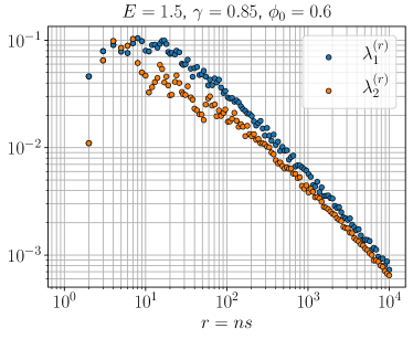
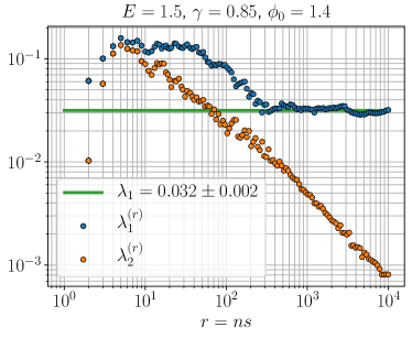
Figure 9: Convergence of the maximum Lyapunov exponent (97) for the Dicke model dynamics in the intermediate regime with a mixed phase space. Here, $E=1.5$, $\gamma=0.5$. Top panel: Regular trajectory with initial condition $\cos\theta_{0}=0.1$ and $\phi_{0}=0.6$. Bottom panel: chaotic trajectory with initial condition $\cos\theta_{0}=0.1$ and $\phi_{0}=1.4$. The parameters and initial conditions chosen here correspond to the two highlighted trajectories in Fig.9. Here we have set $s=1$.

References

- Schrödinger (1935) E. Schrödinger, Mathematical Proceedings of the Cambridge Philosophical Society 31, 555 (1935).
- Wheeler (1998) N. Wheeler, Remarks concerning the status & some ramifications of Ehrenfest’s theorem (1998).
- Berry et al. (1987) M. V. Berry, I. C. Percival, and N. O. Weiss, Proceedings of the Royal Society of London. A. Mathematical and Physical Sciences 413, 183 (1987).
- Gutzwiller (1990) M. C. Gutzwiller, Chaos is classical and quantum mechanics (Springer, 1990).
- Haake (2010) F. Haake, Quantum Signatures of Chaos (Springer Berlin Heidelberg, 2010).
- Zurek and Paz (1994) W. H. Zurek and J. P. Paz, Phys. Rev. Lett. 72, 2508 (1994).
- Zurek and Paz (1995) W. H. Zurek and J. P. Paz, Physica D: Nonlinear Phenomena 83, 300 (1995).
- Kolmogorov (1958) A. N. Kolmogorov, in Doklady Akademii Nauk, Vol. 119 (Russian Academy of Sciences, 1958) pp. 861–864.
- Sinai (1959) I. Sinai, Doklady Akademii Nauk SSSR 124, 768 (1959).
- Pesin (1977) J. B. Pesin, Russ. Math. Surv. 32, 55 (1977).
- Zarum and Sarkar (1998) R. Zarum and S. Sarkar, Phys. Rev. E 57, 5467 (1998).
- Furuya et al. (1998) K. Furuya, M. C. Nemes, and G. Q. Pellegrino, Phys. Rev. Lett. 80, 5524 (1998).
- Miller and Sarkar (1999a) P. A. Miller and S. Sarkar, Nonlinearity 12, 419 (1999a).
- Miller and Sarkar (1999b) P. A. Miller and S. Sarkar, Phys. Rev. E 60, 1542 (1999b).
- Pattanayak (1999) A. K. Pattanayak, Phys. Rev. Lett. 83, 4526 (1999).
- Monteoliva and Paz (2000) D. Monteoliva and J. P. Paz, Phys. Rev. Lett. 85, 3373–3376 (2000).
- Gong and Brumer (2003a) J. Gong and P. Brumer, Phys. Rev. A 68 (2003a).
- Gong and Brumer (2003b) J. Gong and P. Brumer, Phys. Rev. Lett. 90 (2003b).
- Alicki et al. (2004) R. Alicki, A. Łoziński, P. Pakoński, and K. Życzkowski, Journal of Physics A: Mathematical and General 37, 5157–5172 (2004).
- Angelo and Furuya (2005) R. M. Angelo and K. Furuya, Phys. Rev. A 71 (2005).
- Petitjean and Jacquod (2006) C. Petitjean and P. Jacquod, Phys. Rev. Lett. 97, 194103 (2006).
- Ribeiro and Angelo (2010) A. D. Ribeiro and R. M. Angelo, Phys. Rev. A 82 (2010).
- Romero et al. (2008) K. M. F. Romero, J. E. Parreira, L. A. M. Souza, M. C. Nemes, and W. Wreszinski, Journal of Physics A: Mathematical and Theoretical 41, 115303 (2008).
- Casati et al. (2012) G. Casati, I. Guarneri, and J. Reslen, Phys. Rev. E 85 (2012).
- Bonança (2011) M. V. S. Bonança, Phys. Rev. E 83, 046214 (2011).
- Souza et al. (2014) L. Souza, J. Faria, and M. Nemes, Optics Communications 331, 148–153 (2014).
- Znidaric and Prosen (2003) M. Znidaric and T. Prosen, Journal of Physics A: Mathematical and General 36, 2463 (2003).
- Jacquod (2004) P. Jacquod, Phys. Rev. Lett. 92, 150403 (2004).
- Calabrese and Cardy (2005) P. Calabrese and J. Cardy, Journal of Statistical Mechanics: Theory and Experiment 2005, P04010 (2005).
- Latorre et al. (2005) J. I. Latorre, R. Orús, E. Rico, and J. Vidal, Phys. Rev. A 71 (2005).
- Amico et al. (2008) L. Amico, R. Fazio, A. Osterloh, and V. Vedral, Rev. Mod. Phys. 80, 517 (2008).
- Horodecki et al. (2009) R. Horodecki, P. Horodecki, M. Horodecki, and K. Horodecki, Rev. Mod. Phys. 81, 865 (2009).
- Witten (2018) E. Witten, Rev. Mod. Phys. 90, 045003 (2018).
- Ryu and Takayanagi (2006) S. Ryu and T. Takayanagi, Journal of High Energy Physics 2006, 045 (2006).
- Bianchi et al. (2018) E. Bianchi, L. Hackl, and N. Yokomizo, Journal of High Energy Physics 2018, 25 (2018).
- Asplund and Berenstein (2016) C. T. Asplund and D. Berenstein, Annals of Physics 366, 113 (2016).
- Hackl et al. (2018) L. Hackl, E. Bianchi, R. Modak, and M. Rigol, Phys. Rev. A 97, 032321 (2018).
- Greiner et al. (2002a) M. Greiner, O. Mandel, T. W. Hansch, and I. Bloch, Nature 419, 51 (2002a).
- Greiner et al. (2002b) M. Greiner, O. Mandel, T. Esslinger, T. W. Hänsch, and I. Bloch, Nature 415, 39 (2002b).
- Bloch et al. (2008) I. Bloch, J. Dalibard, and W. Zwerger, Rev. Mod. Phys. 80, 885 (2008).
- Trotzky et al. (2008) S. Trotzky, P. Cheinet, S. Fölling, M. Feld, U. Schnorrberger, A. M. Rey, A. Polkovnikov, E. A. Demler, M. D. Lukin, and I. Bloch, Science 319, 295 (2008).
- Cheneau et al. (2012) M. Cheneau, P. Barmettler, D. Poletti, M. Endres, P. Schausz, T. Fukuhara, C. Gross, I. Bloch, C. Kollath, and S. Kuhr, Nature 481, 484 (2012).
- Kaufman et al. (2016) A. M. Kaufman, M. E. Tai, A. Lukin, M. Rispoli, R. Schittko, P. M. Preiss, and M. Greiner, Science 353, 794 (2016).
- Schweigler et al. (2017) T. Schweigler, V. Kasper, S. Erne, I. Mazets, B. Rauer, F. Cataldini, T. Langen, T. Gasenzer, J. Berges, and J. Schmiedmayer, Nature 545, 323 (2017).
- Rauer et al. (2018) B. Rauer, S. Erne, T. Schweigler, F. Cataldini, M. Tajik, and J. Schmiedmayer, Science 360, 307 (2018).
- Albiez et al. (2005) M. Albiez, R. Gati, J. Fölling, S. Hunsmann, M. Cristiani, and M. K. Oberthaler, Phys. Rev. Lett. 95, 010402 (2005).
- Strobel et al. (2014) H. Strobel, W. Muessel, D. Linnemann, T. Zibold, D. B. Hume, L. Pezzè, A. Smerzi, and M. K. Oberthaler, Science 345, 424 (2014).
- Leroux et al. (2010) I. D. Leroux, M. H. Schleier-Smith, and V. Vuletić, Phys. Rev. Lett. 104, 073602 (2010).
- Davis et al. (2019) E. J. Davis, G. Bentsen, L. Homeier, T. Li, and M. H. Schleier-Smith, Phys. Rev. Lett. 122, 010405 (2019).
- Bohnet et al. (2016) J. G. Bohnet, B. C. Sawyer, J. W. Britton, M. L. Wall, A. M. Rey, M. Foss-Feig, and J. J. Bollinger, Science 352, 1297 (2016).
- Gärttner et al. (2017) M. Gärttner, J. G. Bohnet, A. Safavi-Naini, M. L. Wall, J. J. Bollinger, and A. M. Rey, Nature Physics 13, 781 (2017).
- Sciolla and Biroli (2011) B. Sciolla and G. Biroli, Journal of Statistical Mechanics: Theory and Experiment 2011, P11003 (2011).
- Helstrom (1969) C. W. Helstrom, Journal of Statistical Physics 1, 231 (1969).
- Tóth and Apellaniz (2014) G. Tóth and I. Apellaniz, Journal of Physics A: Mathematical and Theoretical 47, 424006 (2014).
- Pezze and Smerzi (2014) L. Pezze and A. Smerzi, arXiv preprint arXiv:1411.5164 (2014).
- Braunstein and Caves (1994) S. L. Braunstein and C. M. Caves, Phys. Rev. Lett. 72, 3439 (1994).
- Petz and Ghinea (2011) D. Petz and C. Ghinea, in Quantum Probability and Related Topics (World Scientific, 2011).
- Pezzè et al. (2018) L. Pezzè, A. Smerzi, M. K. Oberthaler, R. Schmied, and P. Treutlein, Reviews of Modern Physics 90 (2018).
- Hyllus et al. (2012) P. Hyllus, W. Laskowski, R. Krischek, C. Schwemmer, W. Wieczorek, H. Weinfurter, L. Pezzé, and A. Smerzi, Phys. Rev. A 85 (2012).
- Tóth (2012) G. Tóth, Phys. Rev. A 85 (2012).
- Hauke et al. (2016) P. Hauke, M. Heyl, L. Tagliacozzo, and P. Zoller, Nature Physics 12, 778 (2016).
- Gabbrielli et al. (2018) M. Gabbrielli, A. Smerzi, and L. Pezzè, Scientific Reports 8 (2018).
- Pappalardi et al. (2017) S. Pappalardi, A. Russomanno, A. Silva, and R. Fazio, Journal of Statistical Mechanics: Theory and Experiment 2017, 053104 (2017).
- Brenes et al. (2020) M. Brenes, S. Pappalardi, J. Goold, and A. Silva, Phys. Rev. Lett. 124 (2020).
- Kitaev (2015) A. Kitaev, “A simple model of quantum holography,” http://online.kitp.ucsb.edu/online/entangled15/kitaev/ (2015).
- Larkin and Ovchinnikov (1969) A. Larkin and Y. N. Ovchinnikov, Sov Phys JETP 28, 1200 (1969).
- Cotler et al. (2018) J. S. Cotler, D. Ding, and G. R. Penington, Annals of Physics 396, 318 (2018).
- Sekino and Susskind (2008) Y. Sekino and L. Susskind, Journal of High Energy Physics 2008, 065 (2008).
- Hosur et al. (2016) P. Hosur, X.-L. Qi, D. A. Roberts, and B. Yoshida, Journal of High Energy Physics 2016, 4 (2016).
- Nahum et al. (2018) A. Nahum, S. Vijay, and J. Haah, Phys. Rev. X 8 (2018).
- Gärttner et al. (2018) M. Gärttner, P. Hauke, and A. M. Rey, Phys. Rev. Lett. 120 (2018).
- Lewis-Swan et al. (2019) R. Lewis-Swan, A. Safavi-Naini, J. Bollinger, and A. Rey, Nature communications 10, 1581 (2019).
- Lerose and Pappalardi (2020) A. Lerose and S. Pappalardi, Phys. Rev. Research 2 (2020).
- Haake et al. (1987) F. Haake, M. Kuś, and R. Scharf, Zeitschrift für Physik B Condensed Matter 65, 381 (1987).
- Dicke (1954) R. H. Dicke, Phys. Rev. 93, 99 (1954).
- de Aguiar et al. (1992) M. de Aguiar, K. Furuya, C. Lewenkopf, and M. Nemes, Annals of Physics 216, 291 (1992).
- Zhuang et al. (2019) Q. Zhuang, T. Schuster, B. Yoshida, and N. Y. Yao, Phys. Rev. A 99 (2019).
- Ghose et al. (2008) S. Ghose, R. Stock, P. Jessen, R. Lal, and A. Silberfarb, Phys. Rev. A 78, 042318 (2008).
- Safavi-Naini et al. (2018) A. Safavi-Naini, R. Lewis-Swan, J. G. Bohnet, M. Gärttner, K. A. Gilmore, J. E. Jordan, J. Cohn, J. K. Freericks, A. M. Rey, and J. J. Bollinger, Phys. Rev. Lett. 121, 040503 (2018).
- Note (1) Unless permutational symmetry is spontaneously broken or fragmentation phenomena take place Vidal et al. (2004).
- Note (2) In going from Eq. (5\@@italiccorr) to Eq. (7\@@italiccorr), one needs to add terms with equal indices in the sums. Such terms are immaterial for , while they provide corrections to the coefficients of order in higher-spin systems. This small modification does not alter the subsequent analysis and, accordingly, we will simply ignore it.
- Vidal et al. (2004) J. Vidal, R. Mosseri, and J. Dukelsky, Phys. Rev. A 69, 054101 (2004).
- Littlejohn (1986) R. G. Littlejohn, Phys. Rep. 138, 193 (1986).
- Polkovnikov (2010) A. Polkovnikov, Ann. Phys. 325, 1790 (2010).
- Brack and Bhaduri (1997) M. Brack and R. K. Bhaduri, Semiclassical Physics (Addison-Wesley, 1997).
- Chaudhury et al. (2009) S. Chaudhury, A. Smith, B. E. Anderson, S. Ghose, and P. S. Jessen, Nature 461, 768 (2009).
- Ghose and Sanders (2004) S. Ghose and B. Sanders, Phys. Rev. A 70, 062315 (2004).
- Piga et al. (2019) A. Piga, M. Lewenstein, and J. Q. Quach, Phys. Rev. E 99, 032213 (2019).
- Wang et al. (2004) X. Wang, S. Ghose, B. C. Sanders, and B. Hu, Phys. Rev. E 70, 016217 (2004).
- Trail et al. (2008) C. M. Trail, V. Madhok, and I. H. Deutsch, Phys. Rev. E 78, 046211 (2008).
- Kumari and Ghose (2019) M. Kumari and S. Ghose, Phys. Rev. A 99, 042311 (2019).
- Lombardi and Matzkin (2011) M. Lombardi and A. Matzkin, Phys. Rev. E 83, 016207 (2011).
- Stamatiou and Ghikas (2007) G. Stamatiou and D. P. Ghikas, Physics Letters A 368, 206 (2007).
- Madhok et al. (2014) V. Madhok, C. A. Riofrío, S. Ghose, and I. H. Deutsch, Phys. Rev. Lett. 112 (2014).
- Fiderer and Braun (2018) L. J. Fiderer and D. Braun, Nature Communications 9 (2018).
- Pappalardi et al. (2018) S. Pappalardi, A. Russomanno, B. Žunkovič, F. Iemini, A. Silva, and R. Fazio, Phys. Rev. B 98, 134303 (2018).
- Sieberer et al. (2019) L. M. Sieberer, T. Olsacher, A. Elben, M. Heyl, P. Hauke, F. Haake, and P. Zoller, npj Quantum Information 5, 78 (2019).
- Pilatowsky-Cameo et al. (2020) S. Pilatowsky-Cameo, J. Chávez-Carlos, M. A. Bastarrachea-Magnani, P. Stránský, S. Lerma-Hernández, L. F. Santos, and J. G. Hirsch, Phys. Rev. E 101 (2020).
- Note (3) The Dicke model is often used in cavity-QED setups, where photon pumping and leakage require a Lindblad description of the dynamics. Here, we will only be concerned with ideally isolated systems, as relevant, e.g., for trapped-ions experiments.
- Emary and Brandes (2003) C. Emary and T. Brandes, Phys. Rev. E 67, 066203 (2003).
- Lambert et al. (2004) N. Lambert, C. Emary, and T. Brandes, Phys. Rev. Lett. 92, 073602 (2004).
- Lóbez and Relaño (2016) C. Lóbez and A. Relaño, Phys. Rev. E 94, 012140 (2016), arXiv: 1604.06334.
- Sinha and Sinha (2019) S. Sinha and S. Sinha, arXiv:1912.06593 (2019).
- Song et al. (2012) L. Song, J. Ma, D. Yan, and X. Wang, The European Physical Journal D 66, 201 (2012).
- Wang et al. (2014) T.-L. Wang, L.-N. Wu, W. Yang, G.-R. Jin, N. Lambert, and F. Nori, New Journal of Physics 16, 063039 (2014).
- Zhang and Chen (2015) Y.-Y. Zhang and X.-Y. Chen, The European Physical Journal D 69, 241 (2015), arXiv: 1503.03953.
- Mirkhalaf and Smerzi (2017) S. S. Mirkhalaf and A. Smerzi, Phys. Rev. A 95, 022302 (2017).
- Gietka et al. (2019) K. Gietka, J. Chwedeńczuk, T. Wasak, and F. Piazza, Phys. Rev. B 99 (2019).
- Bhattacherjee and Sharma (2016) A. B. Bhattacherjee and D. Sharma, arXiv:1607.01930 (2016).
- Buijsman et al. (2017) W. Buijsman, V. Gritsev, and R. Sprik, Phys. Rev. Lett. 118, 080601 (2017).
- Alavirad and Lavasani (2019) Y. Alavirad and A. Lavasani, Phys. Rev. A 99, 043602 (2019).
- Chávez-Carlos et al. (2019) J. Chávez-Carlos, B. López-del Carpio, M. A. Bastarrachea-Magnani, P. Stránský, S. Lerma-Hernández, L. F. Santos, and J. G. Hirsch, Phys. Rev. Lett. 122, 024101 (2019).
- Note (4) The nonvanishing eigenvalues of are equal to those of .
- Wootters (1981) W. K. Wootters, Phys. Rev. D 23, 357 (1981).
- Pezzè et al. (2017) L. Pezzè, M. Gabbrielli, L. Lepori, and A. Smerzi, Phys. Rev. Lett. 119, 250401 (2017).
- Hiroshima (2001) T. Hiroshima, Phys. Rev. A 63, 022305 (2001).
- Wineland et al. (1992) D. J. Wineland, J. J. Bollinger, W. M. Itano, F. L. Moore, and D. J. Heinzen, Phys. Rev. A 46, R6797 (1992).
- Ma et al. (2011) J. Ma, X. Wang, C. Sun, and F. Nori, Physics Reports 509, 89 (2011).
- Sørensen and Mølmer (2001) A. S. Sørensen and K. Mølmer, Phys. Rev. Lett. 86, 4431 (2001).
- Sørensen et al. (2001) A. Sørensen, L.-M. Duan, J. I. Cirac, and P. Zoller, Nature 409, 63 (2001).
- Pezzé and Smerzi (2009) L. Pezzé and A. Smerzi, Phys. Rev. Lett. 102, 100401 (2009).
- Jalabert et al. (2018) R. A. Jalabert, I. García-Mata, and D. A. Wisniacki, Phys. Rev. E 98, 062218 (2018).
- Rozenbaum et al. (2017) E. B. Rozenbaum, S. Ganeshan, and V. Galitski, Phys. Rev. Lett. 118, 086801 (2017).
- Craps et al. (2019) B. Craps, M. De Clerck, D. Janssens, V. Luyten, and R. Charles, arXiv:1908.08059 (2019).
- Rozenbaum et al. (2019a) E. B. Rozenbaum, L. A. Bunimovich, and V. Galitski, arXiv preprint arXiv:1902.05466 (2019a).
- Rammensee et al. (2018) J. Rammensee, J. D. Urbina, and K. Richter, Phys. Rev. Lett. 121 (2018).
- Rautenberg and Gärttner (2019) M. Rautenberg and M. Gärttner, arXiv preprint arXiv:1907.04094 (2019).
- Prakash and Lakshminarayan (2019) R. Prakash and A. Lakshminarayan, arXiv preprint arXiv:1904.06482 (2019).
- Pappalardi et al. (2020) S. Pappalardi, A. Polkovnikov, and A. Silva, SciPost Physics 9 (2020).
- Schmitt et al. (2019) M. Schmitt, D. Sels, S. Kehrein, and A. Polkovnikov, Phys. Rev. B 99, 134301 (2019).
- Wang et al. (2019) J. Wang, G. Benenti, G. Casati, and W. Wang, arXiv preprint arXiv:1912.07043 (2019).
- Gharibyan et al. (2019) H. Gharibyan, M. Hanada, B. Swingle, and M. Tezuka, Journal of High Energy Physics 2019 (2019).
- Rozenbaum et al. (2019b) E. B. Rozenbaum, S. Ganeshan, and V. Galitski, Phys. Rev. B 100 (2019b), 10.1103/physrevb.100.035112.
- Yan and Chemissany (2020) B. Yan and W. Chemissany, arXiv preprint arXiv:2004.03501 (2020).
- Cencini et al. (2010) M. Cencini, F. Cecconi, and A. Vulpiani, Chaos: from simple models to complex systems (World Scientific, 2010).
- Note (5) In the absence of a standard terminology.
- Oseledets (1968) V. I. Oseledets, Trans. Moscow Math. Soc. 19, 197 (1968).
- Benettin et al. (1976) G. Benettin, L. Galgani, and J.-M. Strelcyn, Phys. Rev. A 14, 2338 (1976).
- Benettin et al. (1980a) G. Benettin, L. Galgani, A. Giorgilli, and J.-M. Strelcyn, Meccanica 15, 9 (1980a).
- Benettin et al. (1980b) G. Benettin, L. Galgani, A. Giorgilli, and J.-M. Strelcyn, Meccanica 15, 21 (1980b).
- Note (6) Subtleties related to the ordering of the operators are not relevant in the following discussion.
- Benatti et al. (2017) F. Benatti, F. Carollo, R. Floreanini, and H. Narnhofer, Journal of Physics A: Mathematical and Theoretical 50, 423001 (2017).
- Dusuel and Vidal (2004) S. Dusuel and J. Vidal, Phys. Rev. Lett. 93, 237204 (2004).
- Lerose et al. (2018) A. Lerose, J. Marino, B. Žunkovič, A. Gambassi, and A. Silva, Phys. Rev. Lett. 120, 130603 (2018).
- Lerose et al. (2019a) A. Lerose, B. Žunkovič, J. Marino, A. Gambassi, and A. Silva, Phys. Rev. B 99, 045128 (2019a).
- Lerose et al. (2019b) A. Lerose, J. Marino, A. Gambassi, and A. Silva, Phys. Rev. B 100, 104306 (2019b).
- Wannier (1966) G. H. Wannier, Statistical Physics (Dover, 1966).
- Note (7) When bipartitions of a permutationally invariant system are considered, one has , where is the number of collective degrees of freedom [cf. Secs.III.1, III.3].
- Vidal J. and Barthel (2007) D. S. Vidal J. and T. Barthel, Journal of Statistical Mechanics: Theory and Experiment 2007, P01015 (2007).
- Note (8) From the correlation matrix , one defines , where is the symplectic unit. The matrix restricted to can be shown to have pairs of opposite real eigenvalues (with as follows from the Heisenberg relations). The are referred as the symplectic eigenvalues of and determine the entanglement entropy via Eq.(45\@@italiccorr).
-
Note (9)
Explicitly,
. - Homrighausen and Kehrein (2019) I. Homrighausen and S. Kehrein, arXiv preprint arXiv:1908.02596 (2019).
- Weedbrook et al. (2012) C. Weedbrook, S. Pirandola, R. García-Patrón, N. J. Cerf, T. C. Ralph, J. H. Shapiro, and S. Lloyd, Rev. Mod. Phys. 84, 621 (2012).
- Note (10) The presence of instead of the identity matrix is immaterial for the definition of the Lyapunov exponents: these are intrinsic quantities associated with the flow that do not depend on the arbitrary choice of the phase-space metric.
- Sorelli et al. (2019) G. Sorelli, M. Gessner, A. Smerzi, and L. Pezzè, Phys. Rev. A 99 (2019).
- Pöschel (2009) J. Pöschel, arXiv:0908.2234 (2009).
- Choi et al. (2019) S. Choi, C. J. Turner, H. Pichler, W. W. Ho, A. A. Michailidis, Z. Papić, M. Serbyn, M. D. Lukin, and D. A. Abanin, Phys. Rev. Lett. 122, 220603 (2019).
- Ho et al. (2019) W. W. Ho, S. Choi, H. Pichler, and M. D. Lukin, Phys. Rev. Lett. 122 (2019).
- Note (11) In fact, the stationary states after a quantum quench explore all the allowed Hilbert space, and their entanglement is upper-bounded by . In collective models under consideration here, however, the conservation of the collective spin magnitude reduces the dimension of the allowed Hilbert space to .
- Page (1993) D. N. Page, Phys. Rev. Lett. 71, 1291 (1993).
- Loh and Kim (2015) Y. L. Loh and M. Kim, American Journal of Physics 83, 30 (2015).
- Gabbrielli et al. (2019) M. Gabbrielli, L. Lepori, and L. Pezzè, New Journal of Physics 21, 033039 (2019).
- Johansson et al. (2013a) F. Johansson et al., mpmath: a Python library for arbitrary-precision floating-point arithmetic (version 1.1.0) (2013a), http://mpmath.org/.
- Johansson et al. (2012) J. Johansson, P. Nation, and F. Nori, Computer Physics Communications 183, 1760 (2012).
- Johansson et al. (2013b) J. Johansson, P. Nation, and F. Nori, Computer Physics Communications 184, 1234 (2013b).
- Bhosale and Santhanam (2018) U. T. Bhosale and M. S. Santhanam, Phys. Rev. E 98, 052228 (2018).
- Ruebeck et al. (2017) J. B. Ruebeck, J. Lin, and A. K. Pattanayak, Phys. Rev. E 95, 062222 (2017).
- Hallam et al. (2019) A. Hallam, J. G. Morley, and A. G. Green, Nature Communications 10 (2019).
- Michailidis et al. (2020) A. Michailidis, C. Turner, Z. Papić, D. Abanin, and M. Serbyn, Phys. Rev. X 10 (2020).
- Note (12) For simplicity, we assume time-reversal invariance, which results in real matrix elements .
- Note (13) Note that the specific choice of the phase space metric is actually immaterial.