The Sloan Digital Sky Survey Reverberation Mapping Project: Mgii Lag Results from Four Years of Monitoring

Abstract

We present reverberation mapping results for the $\hbox{{\rm Mg}\kern 1.00006pt{\sc ii}}\,\lambda 2800$Å broad emission line in a sample of 193 quasars at $0.35<z<1.7$ with photometric and spectroscopic monitoring observations from the Sloan Digital Sky Survey Reverberation Mapping project during 2014 - 2017. We find significant time lags between the Mgii and continuum lightcurves for 57 quasars and define a “gold sample” of 24 quasars with the most reliable lag measurements. We estimate false-positive rates for each lag that range from 1-24%, with an average false-positive rate of 11% for the full sample and 8% for the gold sample. There are an additional $\sim$40 quasars with marginal Mgii lag detections which may yield reliable lags after additional years of monitoring. The Mgii lags follow a radius – luminosity relation with a best-fit slope that is consistent with $\alpha=0.5$ but with an intrinsic scatter of 0.36 dex that is significantly larger than found for the H$\beta$ radius – luminosity relation. For targets with SDSS-RM lag measurements of other emission lines, we find that our Mgii lags are similar to the H$\beta$ lags and $\sim$2-3 times larger than the Civ lags. This work significantly increases the number of Mgii broad-line lags and provides additional reverberation-mapped black hole masses, filling the redshift gap at the peak of supermassive black hole growth between the H$\beta$ and Civ emission lines in optical spectroscopy.

1 Introduction

Observations over more than two decades have shown that supermassive black holes (SMBHs) exist at the center of every massive galaxy and that several galaxy properties are correlated with the mass of the central SMBH (Magorrian et al., 1998; Gültekin et al., 2009; Kormendy & Ho, 2013). Understanding the “co-evolution” of galaxies and their SMBHs, as implied by these correlations, depends critically on accurately measuring SMBH masses over cosmic time.

The masses of nearby SMBHs have been measured using high spatial resolution observations of stellar or gas dynamics (for a review, see Kormendy & Ho, 2013), or, in one specific case of M87, using the black hole “shadow” (Event Horizon Telescope Collaboration et al., 2019). However, these techniques are not yet possible for higher redshift galaxies (${z\gtrsim 0.3}$) even with next generation facilities. Beyond the local universe, reverberation mapping (RM, e.g. Blandford & McKee, 1982; Peterson, 1993, 2004) is the primary technique for measuring SMBH masses. Nearly all rapidly accreting SMBHs, observed as quasars or broad-line active galactic nuclei (AGN), exhibit widespread variability on timescales of weeks to years (e.g. MacLeod et al., 2012). RM measures the time lag, $\tau$, between the variability in the continuum and the broad emission lines. In the standard “lamp post” model (Cackett & Horne, 2006), this time delay is simply the light travel distance between the central SMBH disk and the broad line-emitting region (BLR). Assuming that the BLR motion is gravitational

$$M_{\rm BH}=\frac{fR_{\rm BLR}\Delta V^{2}}{G}.$$ (1)

Determines the virial product where $G$ is the gravitational constant, $R_{\rm BLR}=c\tau$ is the characteristic size of the BLR, $\Delta V$ is the broad emission line width, and $f$ is a dimensionless factor of order unity that depends (in ways still not fully understood) on the orientation, structure, and geometry of the BLR.

Depending on quasar redshift, different emission lines are used to find the correlation between BLR and continuum lightcurves. The Balmer lines H$\beta$ and H$\alpha$ are well-studied in numerous optical RM observations of broad-line AGN at $z<1$ (Peterson et al., 1991; Kaspi et al., 2000; Peterson, 2004; Bentz et al., 2009, 2010; Denney et al., 2010; Grier et al., 2012; Barth et al., 2015; Du et al., 2015; Hu et al., 2015; Shen et al., 2016a; Du et al., 2016a, b; Grier et al., 2017; Pei et al., 2017), with a total of $\sim$100 mass measurements, mostly at $z<0.3$.

There are an additional $\sim$60 RM measurements of the Civ $\lambda$1549 emission line for quasars at $z>1.3$ (Kaspi et al., 2007; Lira et al., 2018; Hoormann et al., 2019; Grier et al., 2019; Shen et al., 2019a). At intermediate redshifts ($0.7\lesssim z\lesssim 1.5$), $\hbox{{\rm Mg}\kern 1.00006pt{\sc ii}}\,\lambda 2800$Å is the strongest broad line in the observed-frame optical. However, there have been only a handful of successful detections of Mgii lags in higher redshift AGN (Shen et al., 2016a; Lira et al., 2018; Czerny et al., 2019), with many other attempts failing (Trevese et al., 2007; Woo, 2008; Cackett et al., 2015), mostly because the Mgii line is generally less variable than the H$\beta$ broad line (Sun et al., 2015). The limited number of Mgii RM measurements from observed-frame ultraviolet (UV) spectroscopy of nearby AGN show lags that are broadly consistent with the H$\beta$ lags of the same objects (Clavel et al., 1991; Reichert et al., 1994; Metzroth et al., 2006).

RM masses over $1\lesssim z\lesssim 2$ are particularly desirable because these epochs represent the peak of SMBH accretion (e.g. Section 3.2 of Brandt & Alexander, 2015): the current lack of Mgii RM measurements fundamentally limits our understanding of SMBH growth.

RM studies of local AGN have established a correlation between the H$\beta$ broad-line radius and the (host-subtracted) AGN luminosity (Kaspi et al., 2000; Bentz et al., 2013). This enables scaling relations to estimate SMBH masses solely from broad-line width and luminosity (Vestergaard & Peterson, 2006). There have been attempts to calibrate Mgii single-epoch masses derived from the RM-based H$\beta$ radius-luminosity relation in quasars with both broad lines, building analogous single-epoch mass estimators from Mgii (McLure & Jarvis, 2002; Vestergaard & Osmer, 2009; Shen et al., 2011; Bahk et al., 2019). However, these Mgii mass estimators are plagued by bias (Shen & Kelly, 2012), and some aspects of the Mgii variability behavior suggest that an intrinsic Mgii radius-luminosity relation may not exist (Guo et al., 2019). Additional RM studies of Mgii are critically needed to understand if the Mgii line can be used for both single-epoch and RM masses, and in turn if it can be used to complete our understanding of SMBH mass buildup through intermediate redshifts.

In this work we present Mgii lag results from four years of spectroscopic and photometric monitoring by the Sloan Digital Sky Survey Reverberation Mapping (SDSS-RM) project. Section 2 describes the details of the SDSS-RM campaign and sample selection criteria, and our methods of time series analysis and lag identification are presented in Section 3. In Section 4 we present tests of lag reliability that motivate our ultimate lag selection criteria and alias removal. Section 5 presents our final lag results, comparing the measured Mgii lags with the H$\beta$ and Civ lags of the same quasars along with a Mgii $R-L$ relation. Finally, we discuss and summarize our work in Section 6. Throughout this work, we adopt a $\Lambda$CDM cosmology with $\Omega_{\Lambda}=0.7$, $\Omega_{M}=0.3$, and $H_{0}=70$ km s^-1 Mpc^-1.

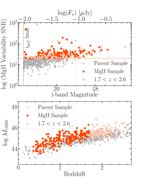
Figure 1: The SDSS-RM parent sample of 849 quasars (gray points) and the Mgii subsample of 193 quasars (red filled points). The Mgii subsample is selected to have significant Mgii variability (top panel; See Section 2.1 for more detail) and redshifts within $0.35<z<1.7$ such that Mgii is in the observed spectral range and uncontaminated by variable sky emission. The open red symbols show $z>1.7$ quasars where the Mgii emission line is variable but frequently affected by telluric contamination. In this paper, all of our analysis is performed on the subsample of 193 targets (filled symbols) with $0.35<z<1.7$.

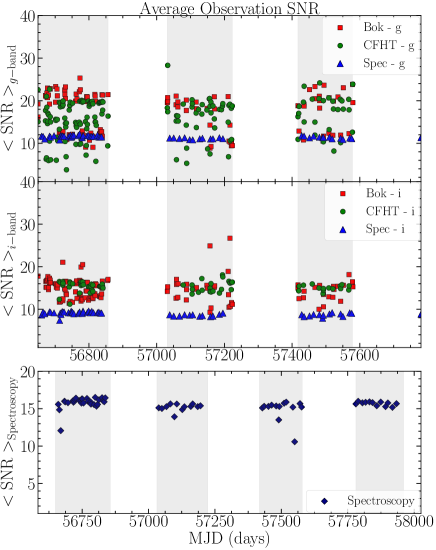
Figure 2: The average SNR and time coverage of the SDSS-RM $g$ (top panel), $i$ (middle panel), and Mgii (bottom panel) monitoring observations. SDSS-RM monitors 849 targets every year from Jan to June 2014 (shaded in gray) with a median spectroscopic cadence of 4 days during the first year. Each point represents the average SNR of the Mgii emission line for the 193 quasars in our Mgii sample observed at that epoch.

2 Data

2.1 Sample Selection

Our sample is drawn from the 849 quasars monitored by SDSS-RM, with spectroscopy and photometry in a single 7 deg² field observed every year from Jan-Jul since 2014 (see Shen et al. 2015a, 2019b). The primary goal of SDSS-RM is to measure lags and black-hole masses for $>$100 quasars spanning a wide range of redshift and AGN properties, using H$\beta$ (Shen et al., 2016a; Grier et al., 2017), Civ (Grier et al., 2019; Shen et al., 2019a), and Mgii (Shen et al., 2016a; this work). SDSS-RM has also been successful in several related studies of quasar variability (Sun et al., 2015; Dexter et al., 2019), quasar emission-line properties (Denney et al., 2016b; Shen et al., 2016b; Denney et al., 2016a; Wang et al., 2019), broad absorption line variability (Grier et al., 2016; Hemler et al., 2019), the relationship between SMBH and host galaxy properties (Matsuoka et al., 2015; Shen et al., 2015b), and quasar accretion-disk lags (Homayouni et al., 2019). SDSS-RM is a purely magnitude-limited sample ($i_{\rm psf}<21.7$ mag), in contrast to previous RM studies that selected samples based on quasar variability, lag detectability, and large emission-line equivalent width. This means that SDSS-RM quasars span a broader range of redshift and other quasar properties compared to previous RM studies (Shen et al., 2015a).

To select the targets for this study, we first require that Mgii is in the observed-frame optical spectra (i.e., $0.35<z<2.6$). After inspecting the SDSS-RM root-mean-square (RMS) spectra, we found that for $\sim 70\%$ of the selected targets with $z>1.7$, the Mgii line profile is weak with respect to the continuum emission and contaminated by (variable) sky lines, and thus we restrict our parent sample to the 453 quasars with $0.35<z<1.7$.

To ensure that Mgii lightcurves are sufficiently variable and have the potential for lag detection, we require a minimum signal-to-noise ratio of the Mgii variability, defined as ${\rm SNR2}\equiv\sqrt{\chi^{2}-DOF}$. Here $\chi^{2}$ is the squared deviation of the fluxes relative to the median with respect to the estimated uncertainties, and ${\rm DOF}=N_{\rm lightcurve}-1$ is the degrees of freedom of each lightcurve. SNR2 quantifies the deviation from the null hypothesis of no variability, where SNR2 $\sim$ 1 indicates that the variability is dominated by the noise. This quantity is calculated by the PrepSpec (Alard & Lupton, 1998) software that is used to flux-calibrate the lightcurves (see Section 2.2 for details). We follow Grier et al. (2019) and require our targets to be significantly variable with ${\rm SNR2}>20$. There are 198 quasars with both $0.35<z<1.7$ and Mgii ${\rm SNR2}>20$. This SNR2 threshold rejects a larger fraction of Mgii targets than it did for the H$\beta$ and Civ samples used in Grier et al. (2017, 2019), as Mgii is generally less variable than the other strong broad lines in quasars (Sun et al., 2015).

Finally, we reject two targets that have Mgii broad absorption lines (BALs) and three targets with weak Mgii emission that have average line fluxes consistent with zero. This results in a Mgii subsample of 193 quasars in which we search for lags. The properties of these targets are summarized in Figure 1, and the details of each target are listed in Table 2.

2.2 Spectroscopy

The SDSS-RM monitoring includes multi-epoch spectroscopy from the BOSS spectrograph (Dawson et al., 2013; Smee et al., 2013) mounted on the 2.5 m SDSS telescope (Gunn et al., 2006), covering wavelengths of 3650-10400 Å with a spectral resolution of $R\sim 2000$. We use four years of SDSS-RM spectroscopic observations, obtained annually during dark/grey observing windows from Jan 2014 to Jul 2017 for a total of 68 spectroscopic epochs. During the first year, SDSS-RM obtained a total of 32 epochs with a median cadence of 4 days for the spectroscopy and 2 days for the photometry discussed below, set by weather conditions and scheduling constraints. The following three years had a sparser cadence, with 12 epochs obtained over the 6-month observing window each year. Figure 2 shows the median SNR of the continuum and Mgii emission line in each epoch for all of the quasars in the Mgii subsample. This SNR is computed from the median ratio of the intercalibrated fluxes and the uncertainties (see 2.4 for more detail) at each epoch.

The spectroscopic data are initially processed through the standard BOSS reduction pipeline (Dawson et al., 2016; Blanton et al., 2017), including flat-fielding, spectral extraction, wavelength calibration, sky subtraction, and flux calibration. The SDSS-RM data are then processed by a secondary custom flux-calibration pipeline that uses position-dependent calibration vectors to improve the spectrophotometric calibrations (see Shen et al., 2015a for details). Finally, PrepSpec is used to further improve the relative spectrophotometry and remove any epoch-dependent calibration errors by optimizing model fits to wavelength-dependent and time-dependent continuum and broad-line variability patterns using the fluxes of the narrow emission lines (see Shen et al., 2016a for details). PrepSpec also computes a maximum-likelihood SNR for the Mgii variability (along with similar variability SNR estimates for the continuum and other emission lines) that is used in our sample selection process (see Section 2.1).

We use the calibrated PrepSpec spectra to compute synthetic photometry in the $g$ and $i$-bands by convolving the calibrated spectra with the SDSS filter response function (Fukugita et al., 1996; Doi et al., 2010). The synthetic flux error is computed using the quadratic sum of errors in the measured spectra, errors in the shape of the response function, and the errors in PrepSpec calibration.

To improve the overall quality of the continuum and line light curves, a small number of epochs ($1\%$) are rejected as outliers if offset from the median flux by more than five times the error-normalized median absolute deviation (NMAD). This outlier rejection effectively removes the rare cases of incorrect fiber placement on the SDSS-RM plates.

2.3 Photometry

SDSS-RM is supported by ground-based photometry from the 3.6 m Canada-France-Hawaii Telescope (CFHT) MegaCam (Aune et al., 2003) and the 2.3 m Steward Observatory Bok telescope 90Prime (Williams et al., 2004) imagers. Photometry was obtained in the $g$ and $i$ filters over the full SDSS-RM field, with the same Jan–Jul time coverage over 2014-2017 and a faster cadence than the spectroscopy. The top panels of Figure 2 show the average SNR of the $g$ and $i$ flux densities at each photometric epoch for the 193 quasars.

The photometric light curves are extracted from the images using image subtraction as implemented in the ISIS software package (Alard, 2000). ISIS aligns all the images and picks a set of images with the best seeing to build a reference image. A scaled reference image, convolved by the point spread function (PSF) at that epoch, is then subtracted from each image to leave only the variable flux. Lightcurves are extracted from the subtracted images and the flux of the quasar in the reference image is added to produce the final lightcurve.

The image subtraction is performed for each individual telescope, filter, CCD and field to produce the $g$ and $i$ lightcurves (Kinemuchi et al. 2020 accepted for publication).

We apply the same outlier rejection method that was implemented on the Mgii lightcurves, removing data points that are more than five times the NMAD from the median lightcurve flux. This step excludes data with incorrect photometry due to clouds, nearby bright stars, or detector edges.

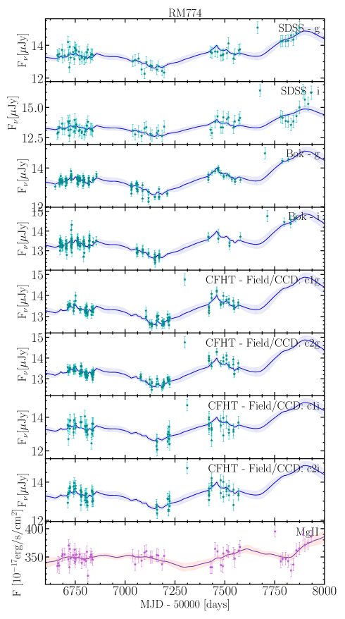
Figure 3: A demonstration of lightcurve intercalibation with CREAM, illustrating model fits and rescaled data for the 4-year lightcurves of RMID 774. Each panel shows the individual pre-merged lightcurve from each observing site in both the $g$ and $i$ filters, the CFHT observations have multiple lightcurves from different fields and CCDs in $\sim$25% of the sample. The CREAM model prediction and rescaled lightcurves are shown for the post-merged data (cyan for continuum lightcurves and pink for emission-line lightcurve).

2.4 Light Curve Merging

Photometric monitoring using three different observing sites ensures that SDSS-RM has sufficient cadence to produce well-sampled continuum lightcurves. However, combining the multi-site observations requires careful treatment of the differences in seeing, calibration, filter response, telescope throughput, and other site-dependent properties. We use CREAM (Continuum REprocessing AGN Markov chain Monte Carlo; Starkey et al., 2016) to inter-calibrate the lightcurves obtained at different sites, following Grier et al. (2017, 2019). CREAM models the lightcurves using a power-law prior for the shape of the lightcurve power spectrum, which resembles the observed behavior of AGN lightcurves on short timescales (MacLeod et al., 2010; Starkey et al., 2016). To inter-calibrate the lightcurves, the CREAM model is fit to the individual photometric lightcurves from each telescope, filter, and pointing, using a delta-function transfer function and zero lag. Each lightcurve is then rescaled and matched to the model using a multiplicative and additive factor, including rescaled flux uncertainties.

The $g$ and $i$ photometry are merged into a single continuum lightcurve, since the lag between these continuum bands is negligible compared to the expected Mgii emission line lags (e.g., Fausnaugh et al., 2016). We additionally use CREAM to rescale the Mgii lightcurve uncertainties, with extra variance as an additive component and a scale factor as a multiplicative component added in quadrature, while allowing the lag and transfer function to be free parameters. An example of the CREAM lightcurve merging is shown in Figure 3.

Occasionally, the photometric $g$ and $i$ lightcurves are affected by contamination from broad emission-line variability. We computed the broad-line variability contamination for the Mgii parent sample and identify 4 targets that have $>$10% contamination in the $g$-band and 5 (different) targets that have $>$10% contamination in the $i$-band. These broad-line contaminated lightcurves are excluded from the merged continuum lightcurves.

We additionally reject photometric lightcurves from individual pointing/CCDs that are visual outliers compared to the other photometric lightcurves of the same object. These rejected outlier lightcurves are generally associated with imaging problems associated with detector edges, and represent $<$1% of the observed lightcurves.

3 Time series analysis

We measure lags from the SDSS-RM lightcurves following the same approach as Grier et al. (2019), with two widely used time series analysis methods adapted for multi-year observations: JAVELIN (Zu et al., 2011) and CREAM (Starkey et al., 2016). We do not use the older Interpolated Cross Correlation Function (i.e., ICCF) method (Gaskell & Sparke, 1986; Gaskell & Peterson, 1987; Peterson, 2004) that was commonly used in previous RM studies. ICCF relies on linear interpolation and is less reliable than JAVELIN and CREAM when applied to SDSS-RM and similar RM programs with sparsely sampled monitoring (Grier et al., 2017; Li et al., 2019), and ICCF also generally overestimates lag uncertainties (Yu et al., 2020). For comparison with ICCF lag measurements, we calculate the Pearson coefficient $r$ between the linearly interpolated continuum and emission line lightcurves (bottom left panel of Figure 4).

3.1 JAVELIN

JAVELIN (Zu et al., 2011) assumes that the quasar variability lightcurve can be modeled by a damped random walk (DRW) process. The DRW description of quasar stochastic variability is well-motivated by observations (Kelly et al., 2009; MacLeod et al., 2010, 2012; Kozłowski, 2016) for the variability timescales probed by SDSS-RM. JAVELIN uses a Markov chain Monte Carlo approach using a maximum likelihood method to fit a DRW model to the continuum and emission-line lightcurves, assuming that the line lightcurve is a shifted, scaled, and smoothed version of the continuum lightcurve.

We allow the DRW amplitude to be a free parameter but fix the DRW damping timescale to 300 days since this quantity is not well constrained by the SDSS-RM monitoring duration. We also tested damping timescales of 100, 200 and 500 days and found no significant differences in the measured lags (as expected; e.g. Yu et al. 2020). The response of the line lightcurve is parameterized as a top-hat transfer function, assuming a lag and scale factor that is a free parameter with a fixed transfer function width of 20 days. Our observations are not sufficient to constrain the width of transfer-function, resulting in unphysical transfer function widths if left as a free parameter in JAVELIN. A 20-day transfer function width is sufficiently short compared to the expected lag. We tested transfer function widths of 10 and 20 days, motivated by velocity resolved lag observations (Grier et al., 2013; Pancoast et al., 2018), with no significant differences in the measured lags. A broader transfer function width of 40 days resulted in significantly different lags for only $\sim$10% of our sample. We adopt a lag search range of $\pm$1000 days, chosen to be less than the $\sim$1300 day monitoring duration from Jan 2014 to Jul 2017. JAVELIN returns a lag posterior distribution from 62500 MCMC simulations which is used to compute the lag and its uncertainty.

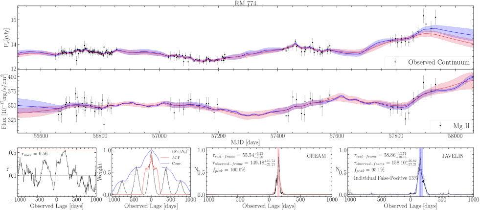
Figure 4: Continuum lightcurve (top panel) and Mgii lightcurve (middle panel) for RM ID 774 along with lag posteriors (bottom panels). In the top two panels both JAVELIN (blue) and CREAM (red) model fits are shown for the continuum and Mgii line lightcurves. The displayed lightcurves are plotted with nightly averages for clarity, although the time-series analysis is computed from the non-averaged observations. Bottom Left: The cross correlation coefficient computed between the continuum and Mgii line lightcurve with its maximum displayed by a horizontal red line. Second from the left: The applied weights for our alias removal, with the $[N(\tau)/N(0)]^{2}$ overlap between lightcurves in black, the continuum auto-correlation function in red, and the final applied weight in blue, obtained from the convolution of the black and red curves. Third and fourth from the left: The unweighted (gray) and weighted (black) lag PDFs computed by JAVELIN and CREAM. The colored curves indicate the smoothed lag PDFs which are used to find the lag bins. The primary lag is indicated by the colored vertical line with its 16th/84th percentile uncertainties enclosed by the colored shading. Available as a Figure Set for the full sample of 193 AGN.

3.2 CREAM

CREAM (Starkey et al., 2016) models the driving lightcurve variability with a random walk power spectrum prior $P(f)\propto f^{-2}$, motivated by the lamp post model (Cackett et al., 2007). The observed continuum lightcurves are only a proxy for the ionizing continuum, and so CREAM constructs a new driving lightcurve and models both the observed continuum and line emission as smoothed versions of this ionizing continuum model. CREAM fits a top-hat response function to the emission-line lightcurve, returning a lag posterior probability distribution while simultaneously inter-calibrating the lightcurves.

Here we use a Python implementation of CREAM called PyceCREAM. We adopt a high frequency variability limit of 0.3 cycles per day and normal priors of $\mathcal{N}$(1.2, 0.2) for the multiplicative error rescaling parameter and normal priors of $\mathcal{N}$(0.5, 0.1) for the variance expansion parameter. As with JAVELIN, we allow CREAM to probe a lag search range of $\pm$1000 days.

4 Lag Reliability & Significance

4.1 Lag Identification & Alias Removal

The posterior lag distributions from JAVELIN or CREAM occasionally contain a primary peak accompanied by other less-significant peaks. The presence of multiple peaks in the posterior lag distribution, also known as aliasing, is a potential outcome of lag detection with sparse sampling data. Aliasing can be caused by matches of weak variability features between the continuum and line lightcurves, because the lag detection MCMC algorithm does not converge, and/or by quasi-periodic variations. The presence of seasonal gaps in multi-year RM data might also cause the lag detection algorithm to inappropriately prefer lags that fall in seasonal gaps where the lightcurve is interpolated with the DRW model prediction in JAVELIN or CREAM rather than directly constrained by observations.

To address the aliasing, we adopt the same lag identification and alias removal procedures of Grier et al. (2019) based on applying a weight to the posterior lag distribution. The weight prior avoids aliased solutions by penalizing parts of the lag posterior that have little overlap between the observed continuum and emission-line lightcurves. This ensures that the final lag search range and lag uncertainties correspond to observationally-motivated lags.

There are two components to the weight prior. For the first component we use the number of overlapping observed epochs between each target’s continuum and line lightcurve, given a time lag $\tau$. If this lightcurve shift results in fewer overlaps between the observed continuum and line lightcurves (e.g., time lags of $\sim$180 days), it is less probable for the lag to be recovered, while more overlapping data points lead to a more secure lag detection. Following Grier et al. (2019) we adopt the overlapping probability weight $P(\tau)=[N(\tau)/N(0)]^{2}$, where $N(\tau)$ corresponds to the number of overlapping continuum lightcurve and $\tau$-shifted line lightcurve points and $N(0)$ is the number of overlapping data points with no lag, i.e., $\tau=0$. We force the weight prior to be symmetric by computing $P(\tau)$ for the line lightcurve shifted by $\tau>0$ with respect to the continuum and then assigning the same values at $\tau=-\tau$.

The second component of the weight prior uses the auto-correlation function (ACF) as a measure of how the continuum variability behavior affects our ability to detect lags. For example, a narrow auto-correlation function indicates rapid variability, in which case seasonal gaps are likely to have consequential effects on our lag detection sensitivity. The final weight prior is the convolution between the overlapping probability, $P(\tau)$, and the continuum lightcurve ACF (forcing $\mathrm{ACF}=0$ when it drops below zero). We refer to the application of the final weight to the posterior lag distributions of JAVELIN and CREAM as the weighted lag posteriors.

To identify the time lag from the weighted posterior lag distribution we first smooth the weighted posteriors by a Gaussian filter with a width of 12 days, which helps to identify the peaks in the weighted lag posteriors. The primary peak in the weighted and smoothed lag posteriors are identified from the peak with the largest area, and smaller ancillary peaks in the lag posterior are considered insignificant for our lag identification. Within this primary peak, the expected lag, $\tau$, is determined from the median of the unweighted lag posteriors and the lag uncertainty is calculated from the 16^th and 84^th percentiles. Figure 4 provides an example of our alias removal approach and lag detection.

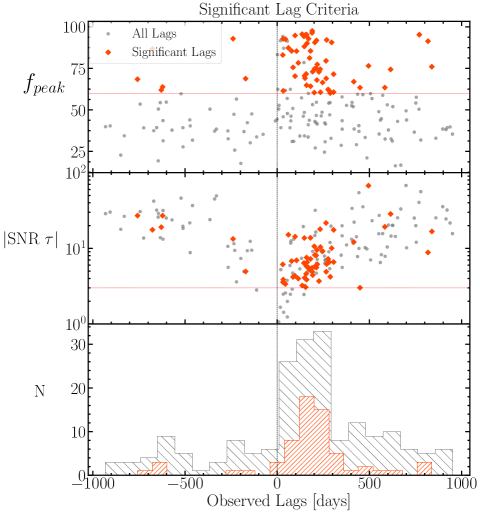
Figure 5: The lag significance criteria for the JAVELIN-measured lags. Top: The fraction of the lag posterior within the primary peak, $f_{peak}$. Middle: The absolute value of the lag SNR. Bottom: The histogram of measured lags for the full sample of 193 AGN (gray) and the sample of significant lags (red). The sample includes 57 significant and positive lags that meet both the $f_{peak}$ and $|\mathrm{SNR}|$ criteria (red lines in the top 2 panels, defined in Section 4.2), with an average false-positive rate of 11%.

4.2 “Significant” Lag Criteria

Our lag identification approach removes many secondary peaks and aliases. We require several additional criteria to ensure the final reported lags are statistically meaningful, following a similar approach to Grier et al. (2019). The first criterion is to require that 60% of the weighted lag posteriors samples are within the primary peak, i.e. $f_{\rm peak}>60\%$. The primary peak, defined in the previous subsection, is the region of the smoothed lag posterior between local minima with the largest area. The $f_{\rm peak}$ requirement ensures a reliable lag solution and removes cases with many alias lags in the posterior. We also require significant lags to be well-detected as 3$\sigma$ different from zero, $|\tau|>3\sigma_{\tau}$.

In summary, our criteria for statistically meaningful lags are:

• $f_{peak}>60\%$: A primary lag peak that includes at least 60% of the weighted lag posterior samples.

• $|\rm SNR(\tau)|>3$: Minimum of 3$\sigma$ difference from zero lag between the absolute value of the measured lag and its uncertainty. If the lag is positive the noise is the lower-bound uncertainty and if the lag is negative the noise is the upper-bound uncertainty.

Figure 5 shows the lag-measurement results for all 193 of our targets. The lag-significance criteria are shown in each panel. There are 63 Mgii lags that meet the significant lag criteria, with 57 positive lags (shown as red points in Figure 5). Table 2 reports the properties of these 57 quasars, drawn from Shen et al. (2019b).

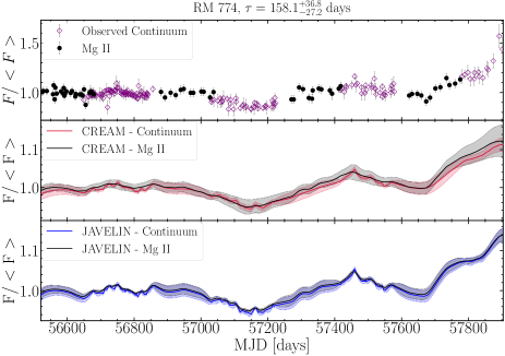
Figure 6: The overlapping continuum and Mgii lightcurves and best-fit CREAM and JAVELIN models for RM 774, with the Mgii lightcurve shifted by the measured lag. In this example the lag is 158 days, such that the shifted Mgii observations fall within the seasonal gap of the continuum observations. However, the lag remains significant and well-constrained because the lightcurve has slow variations on multi-year timescales, such that the lag corresponds to periods in which both the continuum and shifted-Mgii lightcurves are both varying in low or high flux states. Available as a Figure Set for the sample of 57 significant positive lags.

As an additional check on the measured lags, Figure 6 presents the overlapping continuum and lag-shifted Mgii lightcurves and the CREAM and JAVELIN model fits. The overlapping lightcurves are especially instructive for lags of $\sim$180 days in which the shifted Mgii observations fall in the seasonal gap of the photometric observations, casting doubt on the reliability of the lag detection. In general these lags are associated with lightcurves that have smooth, low-frequency variations on multi-year timescales, like the example shown. In such cases the lag posterior is well-constrained with a strong primary peak corresponding to when both the continuum and shifted Mgii lightcurves are in low or high flux states. Significant lag detections of $\sim$180 days can only be found for slow-varying lightcurves like the example shown in Figure 6. Lightcurves with variations on short timescales (i.e. high-frequency variability) require more overlap between shifted lightcurves for significant lag detection. Similar results have also been reported by Shen et al. (2019a) for Civ lightcurves.

4.3 Rate of False-Positive Lags and “Gold Sample”

Large RM survey programs like SDSS-RM will inevitably include some number of false-positive lag detections. In particular, the limited cadence and seasonal gaps might allow for lag PDFs with well-defined peaks that meet our significant lag criteria but result from superpositions of non-reverberating lightcurves rather than genuine reverberation. We estimate the average false-positive rate of our lag detections by using the fact that our lag detection analysis does not include any preference for positive versus negative lags, with a lag search range and weighted prior that are both symmetric over $-1000<\tau<1000$ days. If the sample included only non-reverberating lightcurves and lag detections from spurious overlapping lightcurves, the number of positive and negative lag detections would be equal. On the other hand, genuine broad-line reverberation should produce only positive lags.

Our sample includes a total of 6 negative and 57 positive lags that meet the significance criteria defined in Section 4.2. The negative lags are likely the result of spurious lightcurve correlations rather than broad-line reverberation, and the symmetric nature of our lag analysis means there is likely a similar number of spurious positive lags. Thus we use the ratio of negative to positive lag detections as an estimate of the average false-positive rate: with 6 negative and 57 positive lags, the false-positive rate is 11%.

Figure 5 demonstrates that our sample includes significantly more positive than negative lags even for lags below our significance criteria ($f_{\rm peak}>60\%$ and $|\mathrm{SNR}(\tau)|>3$). In the full sample, there are 149 positive and 44 negative lags, indicating an overall false-positive rate of 30%. The larger number of positive lags in the full sample indicates that an additional 40-50 of the positive lags are likely to be true positive lags. Many of these lower-significance positive lags are likely to become significant detections with additional SDSS-RM monitoring planned as part of the SDSS-V survey (Kollmeier et al., 2019).

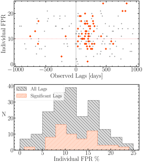
Figure 7: Top: The distribution of individual false-positive rates and measured lags for the full sample (gray) and significant lags (red). False positive rates are measured from matching each quasar continuum lightcurve with Mgii lightcurves of different quasar, repeated 100 times. Bottom: A histogram of false-positive rates measured for full sample (gray) and the sample of significant lags (red). The significant lag sample has an average false-positive rate of 12% from this method, with a “gold sample” of 24 significant and positive lags with false-positive rates of $\leq$10%.

The false-positive rate measured from the ratio of negative to positive lags is a robust indication of the overall sample reliability. However, not all lags in our sample are equally likely to correspond to physical reverberation or spurious correlations. To address this, we design an individual false-positive rate test on all 193 set of lightcurves as a measure of each lag’s likelihood of being true. We measure JAVELIN lag posteriors from each AGN continuum lightcurve matched to the Mgii lightcurve of a different AGN, repeating this process 100 times (and excluding duplications). Since the lightcurves from different AGN are uncorrelated, any lag detections meeting our significance criteria are false positives. The individual false-positive rates for the 57 positive significant lags are reported in Table 2 and shown in Figure 7. The average of the individual false-positive rates for the 57 positive significant lags is 11%, similar to the 11% false-positive rate for the sample measured from the ratio of significant negative to positive lags.

We use the individual false-positive rates to define a “gold sample” of the most reliable lag measurements with individual false-positive rates of $\leq$10%. The gold sample includes 24 significant, positive Mgii lags.

4.4 Lag Comparison: JAVELIN and CREAM

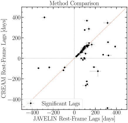
Figure 8: A comparison of lag measurements from JAVELIN and CREAM for the sample of 63 positive and negative lags that meet our significance criteria (defined in Section 4.2). Overall, CREAM and JAVELIN lag measurements are consistent within 1$\sigma$ for 39 of the 63 significant lags (62%), although 33% of the lag solutions are outliers that differ by more than 3$\sigma$. In many of these outlier cases the CREAM model fits find lags of $\sim$0 and/or with multiple peaks in the lag posterior that do not meet our significance criteria; only 13 lags are significant in both JAVELIN and CREAM and differ by more than 3$\sigma$.

We test the reliability of our lag detections by comparing the results of JAVELIN and CREAM, as shown in Figure 8. In general the two methods agree quite well: 60% of the significant JAVELIN lags have CREAM lags that agree within 1$\sigma$. In the full sample of significant positive and negative lags, there are a large number of outliers (21/63) that have JAVELIN and CREAM lags that differ by more than 3$\sigma$.

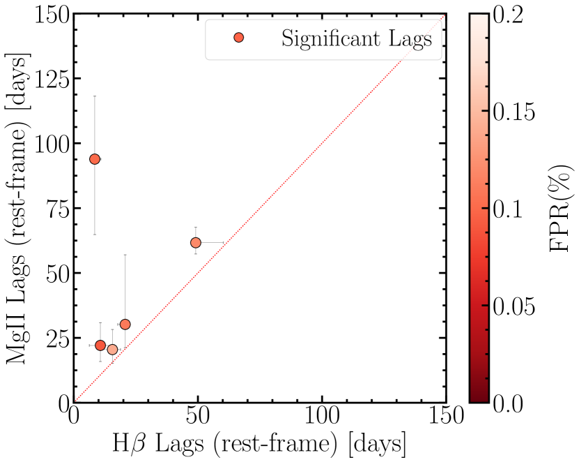
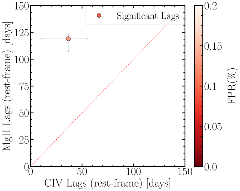
Figure 9: The comparison of 5 Mgii and H$\beta$ lags (left) and 1 Mgii and Civ lags (right) for the quasars with significant lags from both this work and previous SDSS-RM studies (Grier et al., 2017, 2019). Limiting the comparison of Mgii and H$\beta$ lags to the 4 objects with Mgii detectable within the 100-day search range of Grier et al. (2017), the ratio of Mgii to H$\beta$ lags is $1.4\pm 0.4$. The single quasar in the right panel has a ratio of Mgii to Civ lag ratio of $3.2\pm 0.6$. In both cases these comparisons are consistent with a stratified BLR, with the Mgii emission region at significantly larger radii than Civ and at similar or marginally larger radii than H$\beta$.

Visual inspection of the JAVELIN and CREAM model fits leads us to conclude that the JAVELIN results are more reliable. In many (8 out of 21) of the outlier cases where the lags disagree by more than 3$\sigma$, the CREAM lag fit fails to find a significant lag, with a lag posterior centered at $\tau\sim 0$ and/or with multiple peaks and $f_{\rm peak}<60$%. Recent work by Li et al. (2019) using simulated lightcurves similarly shows that JAVELIN typically outperforms other methods of lag identification, with more reliable lag uncertainties and lower false lag detections, for survey-quality RM observations.

We also compare our lag measurements with the 6 Mgii lags measured using only the 2014 SDSS-RM data by Shen et al. (2016a). We only recover the same lag for 1 of these 6 lags as a positive significant lag (RM 457). We find a consistent lag with Shen et al. (2016a) for 2 of the 6 (RM 101 and RM 229), but the lags do not meet our significance criteria because they have $f_{\rm peak}<0.6$. This is not surprising because Shen et al. (2016a) did not use a $f_{\rm peak}$ criterion for measuring lags. The remaining 3 objects (RM 589, RM 767 and RM 789) are more unusual: the 2014 lightcurves appear to be variable with Mgii reverberation, but the other three years have less variability and/or less apparent connection between the Mgii and continuum lightcurves, which result in the non-detection of a Mgii lag using the 4-year data. These may be examples of anomalous BLR variability, sometimes referred to as “holiday states” (Dehghanian et al., 2019; Kriss et al., 2019), where the emission line stops reverberating with respect to the optical continuum.

5 Discussion

5.1 Stratification of the Broad Line Region

Reverberation mapping of multiple emission lines can reveal stratification of the broad-line region. Previous work has generally found that high-ionization lines like Civ and Heii generally have shorter lags (i.e., lie closer to the ionizing continuum) while low-ionization lines like H$\beta$ and H$\alpha$ have longer lags (e.g., Clavel et al., 1991; Peterson & Wandel, 1999; De Rosa et al., 2015). However, while its lower ionization suggests it is more likely to be emitted at larger radii, it is not clear how Mgii fits into the picture of BLR stratification. Unlike the recombination-dominated Balmer lines, the Mgii line includes significant collisional excitation, and is expected to have lower responsivity and a broader response function (Goad et al., 1993; O’Brien et al., 1995; Korista & Goad, 2000; Guo et al., 2020). To date, there have been too few observations of Mgii lags to conclusively understand where the Mgii line sits relative to the rest of the BLR.

We compare our Mgii lags to published SDSS-RM H$\beta$ (Grier et al., 2017) and Civ (Grier et al., 2019) lags in the same quasars in Figure 9. There are 7 quasars with both H$\beta$ and Mgii lags and only 1 quasar with both Civ and Mgii lags. The small number of matches is due in part to the limited redshift range for observing both lines; having both Civ and Mgii is especially limited because we restricted the Mgii sample to $z<1.7$ to avoid variable sky line contamination. The H$\beta$-Mgii lag comparison is further limited by the 100-day search range of the Grier et al. (2017) H$\beta$ lag sample, since it excludes longer H$\beta$ lags that could be observed in quasars with longer Mgii lags.

To avoid this bias, we analysed the 4-year SDSS-RM lightcurves with JAVELIN to estimated H$\beta$ lags for the three quasars with Mgii lags of $>\,$75 days. In one of these cases we find the same lag as Grier et al. (2017), while the other two targets have $f_{\rm peak}<60$% and the Grier et al. (2017) lags are coincident with secondary peaks in the lag posterior. The secondary lag peaks are likely due to additional variability features present in the multi-year data.

Furthermore, the measured lag may be different if the quasar luminosity changed significantly over multiple years of observations. We remove the two sources with low-$f_{\rm peak}$ lags from the comparison and find a Mgii to H$\beta$ lag ratio of $1.4\pm 0.4$ (mean and uncertainty in the mean) for the remaining five objects. This ratio is consistent with the Mgii emitting region being similar in size or marginally larger than the H$\beta$ emission region, and is also broadly consistent with previous Mgii lag measurements (Clavel et al., 1991; Czerny et al., 2019). A full analysis of the H$\beta$ lags measured from the multi-year SDSS-RM data and their comparison to the Mgii lags measured here will appear in future work.

The single quasar with both Mgii and Civ lags, RM158, has a Mgii lag that is $3.2\pm 0.6$ times longer than the Civ lag. The larger Civ lag is consistent with the BLR stratification model, where high-ionization lines such as Civ are at smaller radii compared to the low-ionization Mgii and H$\beta$ lines.

5.2 The Mgii Radius–Luminosity Relation

Previous RM studies of H$\beta$ and Civ have established empirical relations between the broad-line lags and the quasar continuum luminosity (Peterson et al., 2005; Kaspi et al., 2007; Bentz et al., 2013; Du et al., 2016a; Grier et al., 2017; Lira et al., 2018; Hoormann et al., 2019; Grier et al., 2019). These “radius–luminosity” relations have typically found a best-fit $R_{\rm{BLR}}\propto\lambda L^{\alpha}_{\lambda}$ consistent with a slope of $\alpha=0.5$, as expected for a photoionization-driven BLR (Davidson, 1972).

In contrast to H$\beta$ and Civ, there has not yet been a sufficient number of Mgii lag measurements to construct a Mgii $R-L$ relation. Compared to H$\beta$ and Civ, attempts to measure RM Mgii lags have been affected by the smaller-amplitude variability of Mgii and its slower response to the continuum compared to the Balmer lines (i.e. Trevese et al., 2007; Woo, 2008; Hryniewicz et al., 2014; Cackett et al., 2015). So far, there are only $\sim$10 quasars with Mgii lag measurements (Clavel et al., 1991; Metzroth et al., 2006; Lira et al., 2018; Czerny et al., 2019), 6 of which come from the 2014 SDSS-RM observations (Shen et al., 2016a). Czerny et al. (2019) combine all the Mgii lag measurements from the literature and show that they are broadly consistent with the H$\beta$ radius–luminosity relation measured by Bentz et al. (2013) with a slope of $\alpha=0.5$ and a Mgii broad-line size similar to H$\beta$.

We combine our new lag measurements with the existing Mgii lag measurements to fit a $R-L$ relation

$$\log\left(\frac{R_{\rm BLR}}{\rm lt-days}\right)=\beta+\alpha\log\left(\frac{\lambda L_{3000}}{10^{44}{\rm erg~{}s}^{-1}}\right).$$ (2)

To determine the best-fit $R-L$ relation, we use the PyMc3 GLM robust linear regression method, which takes a Bayesian approach to linear regression. We includes an intrinsic scatter, $\sigma$, as a fitted parameter added in quadrature to the observed error. This is similar to the intrinsic scatter model used in the FITEXY method of Kelly (2007).

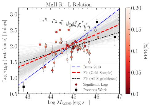
Figure 10: The Mgii $R-L$ relation for our new Mgii lags (circles, color-coded by individual false-positive rate) and previous measurements (black squares, compiled by Czerny et al. 2019). The black cross symbols represent the upper limit in rest-frame lag computed from the observed-frame 1000-day search range and the target’s redshift. The best-fit linear regression to the previous lags and our “gold sample” of lags (with individual false-positive rates of $\leq$10%) is shown by the dashed red line and has a slope of 0.31$\pm$ 0.1, with an excess intrinsic scatter of 0.36 dex. The gray shading indicates several samples of the MCMC fits. The best-fit line is shallower but marginally consistent (within $2\,\sigma$) with the $\alpha=0.533^{+0.035}_{-0.033}$ slope of the Bentz et al. (2013) best-fit H$\beta$ $R-L$ relation, although the Mgii $R-L$ relation has significantly larger scatter. Fitting the entire sample, our 57 significant positive lags results in a shallower $R-L$ relation with a slope of $0.22^{+0.06}_{-0.05}$, although this fit is likely affected by a larger number of false-positive lags than the gold sample.

Figure 10 shows the Mgii radius–luminosity relation for our new measurements and the 3 previous Mgii lags (compiled by Czerny et al. 2019). We use the 24 quasars from the gold sample along with the 3 existing Mgii lag measurements to find a best-fit Mgii radius–luminosity relation with a slope of $\alpha=0.31^{+0.09}_{-0.10}$ and an intrinsic scatter of 0.36 dex (shown as the red line and gray envelope in Figure 10), the Mgii $R-L$ best-fit slope is shallower but still marginally consistent (within $2\sigma$) with the H$\beta$ $R-L$ best-fit line from Bentz et al. (2013), which lies within the uncertainties of our best-fit line in Figure 10. If we use the $F$-test to quantify whether the slope $\alpha$ is necessary to model the data, we find that a luminosity-independent model ($\alpha\equiv 0$) is rejected with a null probability of p = 0.002. This suggests that there exists a $R-L$ relation for the Mgii emission line that is similar to H$\beta$, as expected for the basic photoionization expectation given the similar ionization potentials of H$\beta$ (13.6 eV) and Mgii (15.0 eV). The radius-luminosity fit to all 57 significant positive lags has a shallower slope of $0.22^{+0.06}_{-0.05}$, but is likely affected by a larger number of false-positive lags.

The shallower slope of our Mgii $R-L$ relation is similar to the shorter H$\beta$ lags in SEAMBH and SDSS-RM quasars (Du et al., 2016a; Grier et al., 2017) compared to the Bentz et al. (2013) relation. As observed for the H$\beta$ lags, the shallower best-fit slope may be caused by a range of quasar accretion rates and/or ionization conditions causing shorter Mgii lags (Du & Wang, 2019; Fonseca Alvarez et al., 2019). It is likely that that shallower slope of the Mgii radius–luminosity relation is connected to its large intrinsic scatter, since large intrinsic scatter tends to lead to a shallower best-fit slope (e.g. Shen & Kelly, 2010). On the other hand, Figure 10 shows that the upper limits in rest-frame lag detection (black crosses) are unlikely to affect the measured slope.

The best-fit Mgii $R-L$ relation has a large excess scatter of 0.36 dex, significantly larger (by $>\,$2$\sigma$) than the 0.25 dex excess scatter measured for the SDSS-RM H$\beta$ lags (Fonseca Alvarez et al., 2019). This may be the result of the Mgii line having a significant collisional excitation component and/or a broader radial extent in the BLR (Goad et al., 1993; Korista & Goad, 2000). Mgii is also a resonance line, so there could be radiative transfer effects that do not occur for H$\beta$ line. A broader Mgii $R-L$ relation than H$\beta$ is also consistent with the predictions of the LOC photoionization models of Guo et al. (2020) which shows that the Mgii emitting region is often located where the BLR is truncated and hence less affected by the continuum luminosity.

It would be interesting to investigate whether the lag offset from the Bentz et al. (2013) relation is connected to the Eddington ratio. Similar studies of the H$\beta$ radius–luminosity relation demonstrate that quasars with higher Eddington ratio and/or higher ionization have shorter lags compared to the canonical $R-L$ expectation (Du et al., 2016b; Fonseca Alvarez et al., 2019). However, we note that Eddington ratio self-correlates with both axes of the $R-L$ relation and thus is not an independent quantity. A more suitable approach would be to adopt the relative iron strength as a proxy for Eddington ratio (e.g., Shen & Ho, 2014). Optical Feii strengths are unavailable in the SDSS spectra of most of our Mgii quasars, given their high redshifts, but Martínez-Aldama et al. (2020) instead found a relationship between relative UV Feii strengths and $R-L$ offset. We plan to further investigate how the Mgii $R-L$ relation correlates with other quasar properties in future work.

Our new Mgii lag measurements occupy a convenient range of lags between the previous measurements of short lags in nearby low-luminosity Seyfert 1 AGN (Clavel et al., 1991; Metzroth et al., 2006) and the long lags measured for luminous quasars (Lira et al., 2018; Czerny et al., 2019). Future monitoring of the SDSS-RM field with SDSS-V (Kollmeier et al., 2019) will cover a 10-year monitoring baseline and add a larger number of longer lags from more luminous quasars.

Lag Sample	$\alpha$	$\beta$	Intrinsic Scatter
Significant	$0.22^{+0.06}_{-0.05}$	$-7.95^{+5.52}_{-10.45}$	$0.30^{0.03}_{0.03}$
Gold	$0.31^{+0.10}_{-0.10}$	$-11.69^{+7.34}_{-16.07}$	$0.36^{+0.07}_{-0.05}$

Table 1: Mgii $R-L$ Best Fit

5.3 Black Hole Masses at Cosmic High Noon

Over the last three decades, numerous campaigns have produced about 100 BH mass measurements from H$\beta$ RM of broad-line AGN at $z<0.3$ (e.g., the compilation of Bentz & Katz 2015). Recent multi-object surveys like SDSS-RM have doubled this number, expanding the sample of H$\beta$ RM masses to $z\sim 1$ (Shen et al., 2016a; Grier et al., 2017) and adding a large set of Civ RM masses at $z\sim 2$ (Grier et al., 2019). But there still remains a large gap in RM mass measurements at $1<z<1.5$, where Mgii is the only strong broad line available in an observed-frame optical spectrum. This redshift range is particularly important because the peak of SMBH total mass growth occurs within $1<z<2$ (e.g. Aird et al., 2015).

With so few RM masses available, the bulk of BH masses over cosmic time have been estimated using scaling relations based on the observed H$\beta$ $R-L$ relation, substituting a single-epoch luminosity measurement for the expensive RM $R_{\rm BLR}$. Since the $R-L$ relation is only well-measured for H$\beta$, single-epoch masses applying it to Mgii and Civ requires an additional scaling from H$\beta$ line widths in quasars with both lines (McLure & Jarvis, 2002; Vestergaard & Osmer, 2009; Shen et al., 2011; Trakhtenbrot & Netzer, 2012; Bahk et al., 2019). Even without this additional step, the uncertainty in H$\beta$ single-epoch BH masses is at least 0.4 dex (Vestergaard & Peterson, 2006; Shen, 2013). The recently observed $R-L$ offsets of H$\beta$ lag measurements in more diverse AGN samples adds additional doubt that the H$\beta$ $R-L$ calibrated from previous RM samples describes the broader AGN population (Du et al., 2016a; Fonseca Alvarez et al., 2019). Finally, the previous lack of empirical data on the Mgii $R-L$ relation raises the question of whether SE masses calibrated for H$\beta$ are reliable for application to Mgii.

We compute RM-based BH masses for the 57 quasars with significant positive Mgii lags following Equation 1. Figure 11 shows the new Mgii mass measurements with previous RM $M_{\rm BH}$ from the SDSS-RM and other RM surveys. We use the Mgii $\sigma_{line,rms}$ from PrepSpec for the line width, $\Delta V$, and a virial factor $f=4.47$ from Woo et al. (2015). We follow the same approach as Grier et al. (2019) and compute the $M_{\rm BH}$ uncertainties by adding in quadrature the propagated lag and line width errors with an additional 0.16 dex uncertainty, representing the typical uncertainty of RM-based masses from the uncertain $f$-factor (Fausnaugh et al., 2016). The measured masses span $7.7<\log(M_{\rm BH}/M_{\odot})<9.6$ and are included in Table 2.

Figure 12 compares the RM masses with single-epoch masses computed from the Shen et al. (2011) prescription (available in the SDSS-RM sample characterization catalog; Shen et al. 2019b). The RM and single-epoch masses are consistent within their large uncertainties, with an average ratio of 1.000$\pm$0.003 and an excess scatter of 0.45. The agreement between RM and single-epoch masses is somewhat surprising given the broad scatter in the Mgii radius–luminosity relation (Figure 10) and the multi-step scaling required to derive the Mgii single-epoch masses (e.g. Vestergaard & Osmer, 2009). The agreement indicates that previous single-epoch masses measured from the Mgii line may be reasonable mass estimates within their large uncertainties.

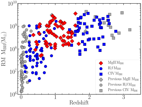
Figure 11: RM $M_{\rm BH}$ vs. redshift for AGNs with RM measurements. Different colored symbols represent the SDSS-RM $M_{\rm BH}$ measurements from H$\beta$ (Grier et al., 2017), Civ (Grier et al., 2019) and Mgii (this work). Gray symbols illustrate the previous RM $M_{\rm BH}$ from the same emission lines (Kaspi et al., 2007; Bentz & Katz, 2015; Du et al., 2016a; Lira et al., 2018; Hoormann et al., 2019; Czerny et al., 2019).

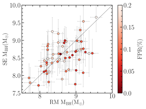
Figure 12: Single-epoch Mgii $M_{\rm BH}$ estimates from Shen et al. (2011) compared to the Mgii $M_{\rm BH}$ measurements from RM. The black dashed line shows a 1:1 ratio and measurements are color coded by the individual false positive rate.

6 Summary

We have used four years of SDSS-RM spectroscopic and photometric monitoring data to measure reverberation lags for the Mgii broad emission line. Starting from a sample of 193 quasars with well-detected Mgii variability (variability ${\rm SNR}>20$) in the redshift range $0.35<z<1.7$, we use JAVELIN to measure significant positive lags in 57 quasars. Comparing the number of positive and negative significant lags suggests an average false-positive rate of 11% for the 57 lags. We additionally measure an individual false-positive rates for each quasar by performing JAVELIN analysis on shuffled continuum and Mgii lightcurves from different objects. We use these false-positive rates to define a “gold sample” of 24 lag measurements with an individual false-positive rate $\leq$10% as our most reliable lag measurements. Our major findings are as follows:

• The new Mgii lags and previous SDSS-RM measurements of H$\beta$ and Civ lags (Grier et al., 2017, 2019) in the same quasars are consistent with a stratified BLR, with Mgii lags that are a factor of a few larger than Civ lags and similar to or slightly larger than H$\beta$ lags.

• We find a radius – luminosity relation for Mgii with a best-fit slope that is shallower but marginally consistent (within $2\,\sigma$) with $\alpha=0.5$, and with 0.4 dex of scatter that is significantly larger than the scatter observed in the H$\beta$ radius – luminosity relation. This implies a broader range of Mgii radii than observed for H$\beta$, consistent with BLR excitation models (Goad et al., 1993; O’Brien et al., 1995; Korista & Goad, 2000; Guo et al., 2020).

• We compute RM-based BH masses for the 57 significant positive lags using the measured Mgii FWHM and find that the single-epoch masses produced by the prescription of Shen et al. (2011) are consistent with the RM masses.

The lack of Mgii RM measurements at the peak of SMBH growth is among the pressing problems in RM measurements. This work provides the first large set of Mgii mass measurements that covers the gap between H$\beta$ and Civ in optical RM studies. Future work will further study BLR stratification using the multi-year SDSS-RM data to measure H$\beta$ lags on a longer monitoring baseline that is comparable to the Mgii lag measurement limits of this work. We will also further investigate the Mgii radius–luminosity relation, using simulations (Li et al., 2019; Fonseca Alvarez et al., 2019) to understand its shallower slope and large scatter.

Table 2: Mgii Significant Lag Results

RMID	$\rm{RA}$	$\rm{DEC}$	$z$	$i$-mag	SNR2	$\log\lambda L_{3000}$	$\tau_{\rm JAV}$	$f_{peak}$	FPR	$\tau_{\rm CREAM}$	log $M_{\rm BH}$	Gold
	deg	deg				log($\rm erg\,s^{-1}$)	(days)	%	%	(days)	($M_{\odot})$	flag
							Rest-Frame			Rest-Frame
018	213.34694	53.1762	0.848	20.21	35	44.4	$125.9^{+6.8}_{-7.0}$	74	14	$112.5^{+7.5}_{-6.2}$	$9.14^{+0.16}_{-0.16}$	0
028	213.92953	52.84914	1.392	19.09	36	45.6	$65.7^{+24.8}_{-14.2}$	71	16	$69.5^{+20.2}_{-15.1}$	$8.51^{+0.23}_{-0.19}$	0
038	214.14908	52.94704	1.383	18.76	35	45.7	$120.7^{+27.9}_{-28.7}$	60	16	$127.0^{+31.5}_{-31.1}$	$8.73^{+0.19}_{-0.19}$	0
044	214.09516	53.30677	1.233	20.56	23	44.9	$65.8^{+18.8}_{-4.8}$	88	8	$-0.2^{+1.0}_{-1.3}$	$8.17^{+0.2}_{-0.16}$	1
102	213.47079	52.57895	0.861	19.54	31	45.0	$86.9^{+16.2}_{-13.3}$	90	13	$88.4^{+17.1}_{-16.8}$	$8.19^{+0.18}_{-0.17}$	0
114	213.89293	53.62056	1.226	17.73	43	46.1	$186.6^{+20.3}_{-15.4}$	67	11	$-85.9^{+7.9}_{-8.9}$	$9.12^{+0.17}_{-0.16}$	0
118	213.55325	52.53583	0.715	19.32	30	45.1	$102.2^{+27.0}_{-19.5}$	81	13	$-578.8^{+5.1}_{-1.7}$	$8.33^{+0.2}_{-0.18}$	0
123	214.65772	53.17155	0.891	20.44	26	44.7	$81.6^{+28.0}_{-26.6}$	95	8	$-14.8^{+17.6}_{-11.5}$	$8.7^{+0.22}_{-0.21}$	1
135	212.79563	52.80433	1.315	19.86	33	45.2	$93.0^{+9.6}_{-9.8}$	68	11	$107.9^{+10.7}_{-14.4}$	$8.22^{+0.17}_{-0.17}$	0
158	214.47802	53.54858	1.478	20.38	20	44.9	$119.1^{+4.0}_{-11.8}$	90	13	$-224.8^{+6.0}_{-4.1}$	$8.75^{+0.16}_{-0.17}$	0
159	213.69478	52.42325	1.587	19.45	34	45.5	$324.2^{+25.3}_{-19.4}$	76	24	$28.1^{+9.0}_{-8.9}$	$9.03^{+0.16}_{-0.16}$	0
160	212.67189	53.31361	0.36	19.68	189	43.8	$106.5^{+18.2}_{-16.6}$	94	16	$46.2^{+16.5}_{-11.2}$	$8.62^{+0.18}_{-0.17}$	0
170	214.52034	53.5496	1.163	20.17	30	45.2	$98.5^{+6.7}_{-17.7}$	91	15	$-3.6^{+4.5}_{-3.7}$	$9.2^{+0.16}_{-0.18}$	0
185	214.39977	52.5083	0.987	19.89	20	44.9	$387.9^{+3.3}_{-3.0}$	95	21	$114.5^{+10.9}_{-9.8}$	$9.36^{+0.16}_{-0.16}$	0
191	214.18991	53.74633	0.442	20.45	24	43.8	$93.9^{+24.3}_{-29.1}$	95	10	$102.1^{+15.0}_{-17.4}$	$8.31^{+0.2}_{-0.21}$	1
228	214.31267	52.38687	1.264	21.25	21	44.7	$37.9^{+14.4}_{-9.1}$	75	17	$37.5^{+5.7}_{-5.6}$	$8.34^{+0.23}_{-0.19}$	0
232	214.21357	52.34615	0.808	20.78	25	44.3	$273.8^{+5.1}_{-4.1}$	76	6	$35.3^{+5.9}_{-5.2}$	$9.0^{+0.17}_{-0.17}$	1
240	213.58696	52.27498	0.762	20.88	34	44.1	$17.2^{+3.5}_{-2.8}$	83	7	$18.6^{+1.5}_{-1.8}$	$8.11^{+0.18}_{-0.18}$	1
260	212.57517	52.57946	0.995	21.64	40	45.3	$94.9^{+18.7}_{-17.2}$	96	16	$3.8^{+4.4}_{-2.7}$	$8.12^{+0.18}_{-0.18}$	0
280	214.95499	53.53547	1.366	19.49	42	45.5	$99.1^{+3.3}_{-9.5}$	60	15	$276.3^{+7.5}_{-9.1}$	$8.51^{+0.16}_{-0.17}$	0
285	214.21215	52.25793	1.034	21.3	22	44.5	$138.5^{+15.2}_{-21.1}$	61	17	$286.8^{+17.5}_{-20.8}$	$8.54^{+0.17}_{-0.17}$	0
291	214.18017	52.24328	0.532	19.82	36	43.8	$39.7^{+4.2}_{-2.6}$	87	19	$40.8^{+3.3}_{-3.1}$	$8.67^{+0.17}_{-0.16}$	0
294	213.42134	52.20559	1.215	19.03	25	45.5	$71.8^{+17.8}_{-9.5}$	64	16	$70.4^{+8.1}_{-6.8}$	$8.37^{+0.19}_{-0.17}$	0
301	215.04269	52.6749	0.548	19.76	58	44.2	$136.3^{+17.0}_{-16.9}$	75	12	$127.0^{+14.1}_{-8.6}$	$9.09^{+0.17}_{-0.17}$	0
303	214.62585	52.37013	0.821	20.88	37	44.2	$57.7^{+10.5}_{-8.3}$	85	10	$55.7^{+9.3}_{-24.0}$	$8.72^{+0.18}_{-0.17}$	1
329	214.249	53.96852	0.721	18.11	47	45.4	$87.5^{+23.8}_{-14.0}$	69	20	$83.8^{+9.4}_{-9.1}$	$8.22^{+0.2}_{-0.18}$	0
338	214.98177	53.66865	0.418	20.08	20	43.8	$22.1^{+8.8}_{-6.2}$	92	9	$22.7^{+8.4}_{-5.5}$	$7.96^{+0.24}_{-0.2}$	1
419	213.00808	52.09101	1.272	20.35	21	45.0	$95.5^{+15.2}_{-15.5}$	77	9	$104.7^{+17.2}_{-21.1}$	$9.15^{+0.17}_{-0.18}$	1
422	211.9132	52.98075	1.074	19.72	31	44.7	$109.3^{+25.4}_{-29.6}$	72	7	$-264.9^{+16.9}_{-25.5}$	$8.99^{+0.19}_{-0.2}$	1
440	215.53806	53.09994	0.754	19.53	37	44.9	$114.6^{+7.4}_{-10.8}$	60	10	$118.7^{+6.7}_{-7.2}$	$9.03^{+0.16}_{-0.17}$	1
441	213.88294	51.98514	1.397	19.35	23	45.5	$127.7^{+5.7}_{-7.3}$	60	8	$126.8^{+3.2}_{-5.4}$	$8.19^{+0.16}_{-0.17}$	1
449	214.92398	53.93835	1.218	20.39	21	45.0	$119.8^{+14.7}_{-24.4}$	68	6	$366.8^{+8.3}_{-6.8}$	$8.9^{+0.17}_{-0.18}$	1
457	213.57136	51.95628	0.604	20.29	29	43.7	$20.5^{+7.7}_{-5.3}$	61	14	$17.6^{+7.0}_{-3.3}$	$7.73^{+0.23}_{-0.2}$	0
459	213.02897	54.14092	1.156	19.95	32	45.0	$122.8^{+5.1}_{-5.7}$	79	8	$-252.6^{+3.5}_{-3.2}$	$9.0^{+0.16}_{-0.16}$	1
469	215.27611	53.73527	1.004	18.31	38	45.6	$224.1^{+27.9}_{-74.3}$	63	24	$-125.4^{+14.4}_{-48.3}$	$9.08^{+0.17}_{-0.22}$	0
492	212.97555	52.0065	0.964	18.95	31	45.3	$92.0^{+16.3}_{-12.7}$	85	17	$94.5^{+11.9}_{-8.0}$	$8.63^{+0.18}_{-0.17}$	0
493	215.16448	52.32457	1.592	18.6	25	46.0	$315.6^{+30.7}_{-35.7}$	91	21	$344.9^{+18.8}_{-14.4}$	$9.56^{+0.17}_{-0.17}$	0
501	214.39663	51.98855	1.155	20.81	22	44.9	$44.9^{+11.7}_{-10.4}$	70	10	$42.9^{+8.6}_{-4.1}$	$8.49^{+0.2}_{-0.19}$	1
505	213.15791	51.95086	1.144	20.58	21	44.8	$94.7^{+10.8}_{-16.7}$	74	9	$95.6^{+11.1}_{-13.3}$	$9.2^{+0.17}_{-0.18}$	1
522	215.1741	52.28379	1.384	20.21	23	45.1	$115.8^{+11.3}_{-16.0}$	62	19	$119.1^{+12.3}_{-12.5}$	$8.26^{+0.17}_{-0.17}$	0
556	215.63556	52.66056	1.494	19.42	25	45.5	$98.7^{+13.9}_{-10.8}$	66	6	$115.5^{+11.9}_{-14.5}$	$8.69^{+0.17}_{-0.17}$	1
588	215.7673	52.77505	0.998	18.64	44	45.6	$74.3^{+23.0}_{-18.2}$	70	11	$60.6^{+12.7}_{-14.6}$	$8.21^{+0.21}_{-0.19}$	0
593	214.09805	51.82018	0.992	19.84	25	45.0	$80.1^{+21.4}_{-20.8}$	95	12	$82.6^{+16.7}_{-14.8}$	$8.03^{+0.2}_{-0.2}$	0
622	212.81328	51.86916	0.572	19.55	37	44.5	$61.7^{+6.0}_{-4.3}$	94	12	$60.0^{+3.9}_{-4.8}$	$7.7^{+0.17}_{-0.16}$	0
645	215.16582	52.06659	0.474	19.78	22	44.2	$30.2^{+26.8}_{-8.9}$	92	11	$26.8^{+15.0}_{-4.5}$	$8.2^{+0.42}_{-0.21}$	0
649	211.47859	52.89651	0.85	20.48	24	44.5	$165.5^{+22.2}_{-25.1}$	71	15	$133.7^{+25.1}_{-24.3}$	$8.8^{+0.17}_{-0.17}$	0
651	215.45543	52.24106	1.486	20.19	32	45.2	$76.5^{+18.0}_{-15.6}$	97	6	$80.9^{+16.0}_{-16.0}$	$8.67^{+0.19}_{-0.18}$	1
675	212.18248	54.13091	0.919	19.46	38	45.1	$139.8^{+12.0}_{-22.6}$	92	6	$149.1^{+3.6}_{-11.7}$	$9.26^{+0.17}_{-0.18}$	1
678	215.26356	52.07418	1.463	19.62	24	45.3	$82.9^{+11.9}_{-10.2}$	90	11	$88.4^{+11.7}_{-11.6}$	$8.52^{+0.17}_{-0.17}$	0
709	212.22948	51.9759	1.251	20.29	25	45.0	$85.4^{+17.7}_{-19.3}$	73	1	$98.4^{+12.7}_{-23.6}$	$8.57^{+0.19}_{-0.19}$	1
714	215.95717	52.65101	0.921	19.64	51	44.8	$320.1^{+11.3}_{-11.2}$	74	8	$157.1^{+8.3}_{-7.8}$	$9.45^{+0.16}_{-0.16}$	1
756	212.34759	51.85559	0.852	20.29	28	44.4	$315.3^{+20.5}_{-16.4}$	63	9	$-485.1^{+8.0}_{-9.7}$	$9.2^{+0.16}_{-0.16}$	1
761	216.05386	52.65096	0.771	20.43	48	44.8	$102.1^{+8.2}_{-7.4}$	64	7	$103.0^{+7.4}_{-6.6}$	$8.82^{+0.16}_{-0.16}$	1
771	214.01893	54.17766	1.492	18.64	42	45.7	$31.3^{+8.1}_{-4.6}$	85	19	$30.5^{+4.4}_{-4.8}$	$8.34^{+0.2}_{-0.17}$	0
774	212.62967	52.05463	1.686	19.34	29	45.7	$58.9^{+13.7}_{-10.1}$	95	13	$55.5^{+6.2}_{-7.9}$	$8.23^{+0.19}_{-0.18}$	0
792	214.503	53.3433	0.526	20.64	23	43.5	$111.4^{+29.5}_{-20.0}$	92	8	$120.3^{+29.2}_{-28.2}$	$8.98^{+0.2}_{-0.18}$	1
848	215.60674	53.57398	0.757	20.81	25	44.1	$65.1^{+29.4}_{-16.3}$	78	10	$58.5^{+15.8}_{-13.5}$	$8.24^{+0.25}_{-0.19}$	1

References

- Aird et al. (2015) Aird, J., Coil, A. L., Georgakakis, A., et al. 2015, MNRAS, 451, 1892
- Alard (2000) Alard, C. 2000, A&AS, 144, 363
- Alard & Lupton (1998) Alard, C., & Lupton, R. H. 1998, ApJ, 503, 325
- Aune et al. (2003) Aune, S., Boulade, O., Charlot, X., et al. 2003, in Society of Photo-Optical Instrumentation Engineers (SPIE) Conference Series, Vol. 4841, Proc. SPIE, ed. M. Iye & A. F. M. Moorwood, 513–524
- Bahk et al. (2019) Bahk, H., Woo, J.-H., & Park, D. 2019, ApJ, 875, 50
- Barth et al. (2015) Barth, A. J., Bennert, V. N., Canalizo, G., et al. 2015, ApJS, 217, 26
- Bentz & Katz (2015) Bentz, M. C., & Katz, S. 2015, Publications of the Astronomical Society of the Pacific, 127, 67
- Bentz et al. (2009) Bentz, M. C., Walsh, J. L., Barth, A. J., et al. 2009, ApJ, 705, 199
- Bentz et al. (2010) —. 2010, ApJ, 716, 993
- Bentz et al. (2013) Bentz, M. C., Denney, K. D., Grier, C. J., et al. 2013, ApJ, 767, 149
- Blandford & McKee (1982) Blandford, R. D., & McKee, C. F. 1982, ApJ, 255, 419
- Blanton et al. (2017) Blanton, M. R., Bershady, M. A., Abolfathi, B., et al. 2017, AJ, 154, 28
- Brandt & Alexander (2015) Brandt, W. N., & Alexander, D. M. 2015, A&A Rev., 23, 1
- Cackett et al. (2015) Cackett, E. M., Gültekin, K., Bentz, M. C., et al. 2015, ApJ, 810, 86
- Cackett & Horne (2006) Cackett, E. M., & Horne, K. 2006, MNRAS, 365, 1180
- Cackett et al. (2007) Cackett, E. M., Horne, K., & Winkler, H. 2007, MNRAS, 380, 669
- Clavel et al. (1991) Clavel, J., Reichert, G. A., Alloin, D., et al. 1991, ApJ, 366, 64
- Czerny et al. (2019) Czerny, B., Olejak, A., Ralowski, M., et al. 2019, arXiv e-prints, arXiv:1901.09757
- Davidson (1972) Davidson, K. 1972, ApJ, 171, 213
- Dawson et al. (2013) Dawson, K. S., Schlegel, D. J., Ahn, C. P., et al. 2013, AJ, 145, 10
- Dawson et al. (2016) Dawson, K. S., Kneib, J.-P., Percival, W. J., et al. 2016, AJ, 151, 44
- De Rosa et al. (2015) De Rosa, G., Peterson, B. M., Ely, J., et al. 2015, ApJ, 806, 128
- Dehghanian et al. (2019) Dehghanian, M., Ferland, G. J., Kriss, G. A., et al. 2019, ApJ, 877, 119
- Denney et al. (2016a) Denney, K. D., Horne, K., Brandt, W. N., et al. 2016a, ApJ, 833, 33
- Denney et al. (2010) Denney, K. D., Peterson, B. M., Pogge, R. W., et al. 2010, ApJ, 721, 715
- Denney et al. (2016b) Denney, K. D., Horne, K., Shen, Y., et al. 2016b, ApJS, 224, 14
- Dexter et al. (2019) Dexter, J., Xin, S., Shen, Y., et al. 2019, arXiv e-prints, arXiv:1906.10138
- Doi et al. (2010) Doi, M., Tanaka, M., Fukugita, M., et al. 2010, AJ, 139, 1628
- Du & Wang (2019) Du, P., & Wang, J.-M. 2019, ApJ, 886, 42
- Du et al. (2015) Du, P., Hu, C., Lu, K.-X., et al. 2015, ApJ, 806, 22
- Du et al. (2016a) Du, P., Lu, K.-X., Zhang, Z.-X., et al. 2016a, ApJ, 825, 126
- Du et al. (2016b) Du, P., Lu, K.-X., Hu, C., et al. 2016b, ApJ, 820, 27
- Event Horizon Telescope Collaboration et al. (2019) Event Horizon Telescope Collaboration, Akiyama, K., Alberdi, A., et al. 2019, ApJ, 875, L6
- Fausnaugh et al. (2016) Fausnaugh, M. M., Denney, K. D., Barth, A. J., et al. 2016, ApJ, 821, 56
- Fonseca Alvarez et al. (2019) Fonseca Alvarez, G., Trump, J. R., Homayouni, Y., et al. 2019, arXiv e-prints, arXiv:1910.10719
- Fukugita et al. (1996) Fukugita, M., Ichikawa, T., Gunn, J. E., et al. 1996, AJ, 111, 1748
- Gaskell & Peterson (1987) Gaskell, C. M., & Peterson, B. M. 1987, ApJS, 65, 1
- Gaskell & Sparke (1986) Gaskell, C. M., & Sparke, L. S. 1986, ApJ, 305, 175
- Goad et al. (1993) Goad, M. R., O’Brien, P. T., & Gondhalekar, P. M. 1993, MNRAS, 263, 149
- Grier et al. (2012) Grier, C. J., Peterson, B. M., Pogge, R. W., et al. 2012, ApJ, 755, 60
- Grier et al. (2013) Grier, C. J., Peterson, B. M., Horne, K., et al. 2013, ApJ, 764, 47
- Grier et al. (2016) Grier, C. J., Brandt, W. N., Hall, P. B., et al. 2016, ApJ, 824, 130
- Grier et al. (2017) Grier, C. J., Trump, J. R., Shen, Y., et al. 2017, ApJ, 851, 21
- Grier et al. (2019) Grier, C. J., Shen, Y., Horne, K., et al. 2019, ApJ, 887, 38
- Gültekin et al. (2009) Gültekin, K., Richstone, D. O., Gebhardt, K., et al. 2009, ApJ, 698, 198
- Gunn et al. (2006) Gunn, J. E., Siegmund, W. A., Mannery, E. J., et al. 2006, AJ, 131, 2332
- Guo et al. (2019) Guo, H., Shen, Y., He, Z., et al. 2019, arXiv e-prints, arXiv:1907.06669
- Guo et al. (2020) —. 2020, ApJ, 888, 58
- Hemler et al. (2019) Hemler, Z. S., Grier, C. J., Brandt, W. N., et al. 2019, ApJ, 872, 21
- Homayouni et al. (2019) Homayouni, Y., Trump, J. R., Grier, C. J., et al. 2019, ApJ, 880, 126
- Hoormann et al. (2019) Hoormann, J. K., Martini, P., Davis, T. M., et al. 2019, MNRAS, 487, 3650
- Hryniewicz et al. (2014) Hryniewicz, K., Czerny, B., Pych, W., et al. 2014, A&A, 562, A34
- Hu et al. (2015) Hu, C., Du, P., Lu, K.-X., et al. 2015, ApJ, 804, 138
- Kaspi et al. (2007) Kaspi, S., Brandt, W. N., Maoz, D., et al. 2007, ApJ, 659, 997
- Kaspi et al. (2000) Kaspi, S., Smith, P. S., Netzer, H., et al. 2000, ApJ, 533, 631
- Kelly (2007) Kelly, B. C. 2007, ApJ, 665, 1489
- Kelly et al. (2009) Kelly, B. C., Bechtold, J., & Siemiginowska, A. 2009, ApJ, 698, 895
- Kollmeier et al. (2019) Kollmeier, J., Anderson, S. F., Blanc, G. A., et al. 2019, in BAAS, Vol. 51, 274
- Korista & Goad (2000) Korista, K. T., & Goad, M. R. 2000, ApJ, 536, 284
- Kormendy & Ho (2013) Kormendy, J., & Ho, L. C. 2013, arXiv e-prints, arXiv:1308.6483
- Kozłowski (2016) Kozłowski, S. 2016, ApJ, 826, 118
- Kriss et al. (2019) Kriss, G. A., De Rosa, G., Ely, J., et al. 2019, ApJ, 881, 153
- Li et al. (2019) Li, J., Shen, Y., Brandt, W. N., et al. 2019, ApJ, 884, 119
- Lira et al. (2018) Lira, P., Kaspi, S., Netzer, H., et al. 2018, ApJ, 865, 56
- MacLeod et al. (2010) MacLeod, C. L., Ivezić, Ž., Kochanek, C. S., et al. 2010, ApJ, 721, 1014
- MacLeod et al. (2012) MacLeod, C. L., Ivezić, Ž., Sesar, B., et al. 2012, ApJ, 753, 106
- Magorrian et al. (1998) Magorrian, J., Tremaine, S., Richstone, D., et al. 1998, AJ, 115, 2285
- Martínez-Aldama et al. (2020) Martínez-Aldama, M. L., Zajaĉek, M., Czerny, B., & Panda, S. 2020, arXiv e-prints, arXiv:2007.09955
- Matsuoka et al. (2015) Matsuoka, Y., Strauss, M. A., Shen, Y., et al. 2015, ApJ, 811, 91
- McLure & Jarvis (2002) McLure, R. J., & Jarvis, M. J. 2002, Monthly Notices of the Royal Astronomical Society, 337, 109
- Metzroth et al. (2006) Metzroth, K. G., Onken, C. A., & Peterson, B. M. 2006, ApJ, 647, 901
- O’Brien et al. (1995) O’Brien, P. T., Goad, M. R., & Gondhalekar, P. M. 1995, MNRAS, 275, 1125
- Pancoast et al. (2018) Pancoast, A., Barth, A. J., Horne, K., et al. 2018, ApJ, 856, 108
- Pei et al. (2017) Pei, L., Fausnaugh, M. M., Barth, A. J., et al. 2017, ApJ, 837, 131
- Peterson (1993) Peterson, B. M. 1993, Publications of the Astronomical Society of the Pacific, 105, 247
- Peterson (2004) Peterson, B. M. 2004, in The Interplay Among Black Holes, Stars and ISM in Galactic Nuclei, ed. T. Storchi-Bergmann, L. C. Ho, & H. R. Schmitt, Vol. 222, 15–20
- Peterson & Wandel (1999) Peterson, B. M., & Wandel, A. 1999, ApJ, 521, L95
- Peterson et al. (1991) Peterson, B. M., Balonek, T. J., Barker, E. S., et al. 1991, ApJ, 368, 119
- Peterson et al. (2005) Peterson, B. M., Bentz, M. C., Desroches, L.-B., et al. 2005, ApJ, 632, 799
- Reichert et al. (1994) Reichert, G. A., Rodriguez-Pascual, P. M., Alloin, D., et al. 1994, ApJ, 425, 582
- Shen (2013) Shen, Y. 2013, Bulletin of the Astronomical Society of India, 41, 61
- Shen & Ho (2014) Shen, Y., & Ho, L. C. 2014, Nature, 513, 210
- Shen & Kelly (2010) Shen, Y., & Kelly, B. C. 2010, ApJ, 713, 41
- Shen & Kelly (2012) —. 2012, The Astrophysical Journal, 746, 169
- Shen et al. (2011) Shen, Y., Richards, G. T., Strauss, M. A., et al. 2011, ApJS, 194, 45
- Shen et al. (2015a) Shen, Y., Brandt, W. N., Dawson, K. S., et al. 2015a, The Astrophysical Journal Supplement Series, 216, 4
- Shen et al. (2015b) Shen, Y., Greene, J. E., Ho, L. C., et al. 2015b, The Astrophysical Journal, 805, 96
- Shen et al. (2016a) Shen, Y., Horne, K., Grier, C. J., et al. 2016a, ApJ, 818, 30
- Shen et al. (2016b) Shen, Y., Brandt, W. N., Richards, G. T., et al. 2016b, ApJ, 831, 7
- Shen et al. (2019a) Shen, Y., Grier, C. J., Horne, K., et al. 2019a, ApJ, 883, L14
- Shen et al. (2019b) Shen, Y., Hall, P. B., Horne, K., et al. 2019b, ApJS, 241, 34
- Smee et al. (2013) Smee, S. A., Gunn, J. E., Uomoto, A., et al. 2013, AJ, 146, 32
- Starkey et al. (2016) Starkey, D. A., Horne, K., & Villforth, C. 2016, MNRAS, 456, 1960
- Sun et al. (2015) Sun, M., Trump, J. R., Shen, Y., et al. 2015, ApJ, 811, 42
- Trakhtenbrot & Netzer (2012) Trakhtenbrot, B., & Netzer, H. 2012, MNRAS, 427, 3081
- Trevese et al. (2007) Trevese, D., Paris, D., Stirpe, G. M., Vagnetti, F., & Zitelli, V. 2007, A&A, 470, 491
- Vestergaard & Osmer (2009) Vestergaard, M., & Osmer, P. S. 2009, ApJ, 699, 800
- Vestergaard & Peterson (2006) Vestergaard, M., & Peterson, B. M. 2006, ApJ, 641, 689
- Wang et al. (2019) Wang, S., Shen, Y., Jiang, L., et al. 2019, ApJ, 882, 4
- Williams et al. (2004) Williams, G. G., Olszewski, E., Lesser, M. P., & Burge, J. H. 2004, in Society of Photo-Optical Instrumentation Engineers (SPIE) Conference Series, Vol. 5492, Proc. SPIE, ed. A. F. M. Moorwood & M. Iye, 787–798
- Woo (2008) Woo, J.-H. 2008, AJ, 135, 1849
- Woo et al. (2015) Woo, J.-H., Yoon, Y., Park, S., Park, D., & Kim, S. C. 2015, ApJ, 801, 38
- Yu et al. (2020) Yu, Z., Kochanek, C. S., Peterson, B. M., et al. 2020, MNRAS, 491, 6045
- Zu et al. (2011) Zu, Y., Kochanek, C. S., & Peterson, B. M. 2011, ApJ, 735, 80