Fast multivariate empirical cumulative distribution function
with connection to kernel density estimation

Abstract

This paper revisits the problem of computing empirical cumulative distribution functions (ECDF) efficiently on large, multivariate datasets. Computing an ECDF at one evaluation point requires $\mathcal{O}(N)$ operations on a dataset composed of $N$ data points. Therefore, a direct evaluation of ECDFs at $N$ evaluation points requires a quadratic $\mathcal{O}(N^{2})$ operations, which is prohibitive for large-scale problems. Two fast and exact methods are proposed and compared. The first one is based on fast summation in lexicographical order, with a $\mathcal{O}(N{\log}N)$ complexity and requires the evaluation points to lie on a regular grid. The second one is based on the divide-and-conquer principle, with a $\mathcal{O}(N\log(N)^{(d-1){\vee}1})$ complexity and requires the evaluation points to coincide with the input points. The two fast algorithms are described and detailed in the general $d$-dimensional case, and numerical experiments validate their speed and accuracy. Secondly, the paper establishes a direct connection between cumulative distribution functions and kernel density estimation (KDE) for a large class of kernels. This connection paves the way for fast exact algorithms for multivariate kernel density estimation and kernel regression. Numerical tests with the Laplacian kernel validate the speed and accuracy of the proposed algorithms. A broad range of large-scale multivariate density estimation, cumulative distribution estimation, survival function estimation and regression problems can benefit from the proposed numerical methods.

Keywords: fast CDF; fast KDE; empirical distribution function; survival function; Laplacian kernel; Matérn covariance; Sargan density; Gaussian kernel approximation; nonparametric copula estimation; fast kernel summation

MSC codes: 65C60; 62G30; 62G07; ACM codes: G.3; F.2.1; G.1.0

1 Introduction

Let $(x_{1},y_{1}),(x_{2},y_{2}),\ldots,(x_{N},y_{N})$ be a sample of $N$ input (source) points $x_{i}=(x_{1,i},x_{2,i},\ldots,x_{d,i})\in\mathbb{R}^{d}$ and output points $y_{i}\in\mathbb{R}$. Consider an evaluation (target) point $z=(z_{1},z_{2},\ldots,z_{d})\in\mathbb{R}^{d}$. We define a generalized multivariate empirical cumulative distribution function (ECDF) as follows:

$$F_{N}(z)=F_{N}(z;x,y)\triangleq\frac{1}{N}\sum_{i=1}^{N}y_{i}\mathbbm{1}\{x_{1,i}\leq z_{1},\ldots,x_{d,i}\leq z_{d}\}\,.$$ (1)

In a similar manner, we define a generalized multivariate empirical survival function (ESF) (a.k.a. complementary cumulative distribution function) as follows:

$$\bar{F}_{N}(z)=\bar{F}_{N}(z;x,y)\triangleq\frac{1}{N}\sum_{i=1}^{N}y_{i}\mathbbm{1}\{x_{1,i}>z_{1},\ldots,x_{d,i}>z_{d}\}\,.$$ (2)

The particular case $y\equiv 1$ corresponds to the classical joint empirical distribution function $F_{N}(z)=\frac{1}{N}\sum_{i=1}^{N}\mathbbm{1}\{x_{1,i}\leq z_{1},\ldots,x_{d,i}\leq z_{d}\}$.

More generally, define the following multivariate ECDF:

$$F_{N}(z,\delta) =F_{N}(z,\delta;x,y)\triangleq\frac{1}{N}\sum_{i=1}^{N}y_{i}\mathbbm{1}\{x_{1,i}\leq_{\delta_{1}}z_{1},\ldots,x_{d,i}\leq_{\delta_{d}}z_{d}\}$$ (3)

where $\delta=\left\{\delta_{1},\delta_{2},\ldots,\delta_{d}\right\}\in\left\{-1,1\right\}^{d}$, and where the generalized inequality operator $\leq_{c}$ corresponds to $\leq$ (lower or equal) if $c\geq 0$, and to $<$ (strictly lower) if $c<0$. In particular $F_{N}(z)=F_{N}(z,1;x,y)$ and $\bar{F}_{N}(z)=F_{N}(-z,-1;-x,y)$ respectively.

Cumulative distribution functions and their empirical counterparts are a cornerstone of statistical theory. In particular, classical statistical tests of equality of probability distributions such as the Kolmogorov-Smirnov, Cramér-von Mises and Anderson-Darling tests are based upon empirical distribution functions (Green  Hegazy, 1976).

The multivariate versions of these tests are methodologically and computationally more involved (Justel . 1997, Chiu  Liu 2009) due to the greater complexity of multivariate ECDFs (1) compared to their univariate counterpart.

A copula is a particular case of multivariate cumulative distribution function with uniform marginals (Durante  Sempi, 2010). Empirical copulas appear in the computation of multivariate measures of association (generalizing the bivariate Spearman rho, Schmid  Schmidt 2007, Schmid . 2010).

The focus of this article is on the numerical computation of generalized multivariate empirical cumulative distribution functions as defined in equation (3). As the computation of the ECDF (3) at one evaluation point $z$ requires $\mathcal{O}(N)$ operations, a direct implementation of equation (3) on a set of $M$ evaluation points requires $\mathcal{O}(M\times N)$ operations. In particular, when the evaluation points coincide with the input points $x_{1},x_{2},\ldots,x_{N}$, a direct evaluation requires a quadratic $\mathcal{O}(N^{2})$ operations.

The main contribution of this article is to propose an exact $\mathcal{O}(N\log N)$ algorithm to perform this task, based on independent data sorting in each dimension, combined with a fast lexicographical-sweep summation algorithm (subsection 2.1). Should the input data be already sorted, the computational complexity is reduced to an optimal $\mathcal{O}(N)$. This new algorithm is compared with the state-of-the-art for fast multivariate ECDF computation, namely the fast divide-and-conquer recursion of Bentley (1980) with $\mathcal{O}(N\log(N)^{(d-1){\vee}1})$ computational complexity (subsection 2.2).

The second main contribution of this article is to establish that a large class of kernel density estimators can be decomposed into a sum of ECDFs (subsection 3.1), which yields an exact $\mathcal{O}(N\log N)$ kernel density estimation approach in the lines of Langrené  Warin (2019), as well as a novel $\mathcal{O}(N\log(N)^{(d-1){\vee}1})$ kernel density estimation algorithm based on the divide-and-conquer approach of Bentley (1980). The table below summarizes the contributions of this paper.

Contributions	multivariate CDF	multivariate KDE
fast summation	this paper	Langrené  Warin (2019)
divide-and-conquer	Bentley (1980)	this paper

The class of compatible kernels contain popular kernels such as the uniform, Epanechnikov and Laplacian kernels (subsection 3.2). It also contains a large class of polynomial-exponential kernels which can be used to uniformly approximate any incompatible kernel such as the Gaussian kernel to arbitrary precision (subsection 3.3).

The numerical tests reported in Section 4 illustrate the speed and accuracy of the proposed numerical methods. In practice, the fast summation algorithm requires the evaluation points to lie on a rectilinear grid, while the divide-and-conquer algorithm requires the evaluation points to be the same as the input points. These constraints mean that depending on the chosen algorithm and the set of evaluation points, an additional interpolation of the results might be necessary, the impact of which on accuracy can be deemed acceptable (Figures 3 and 5 in Section 4).

The contributions of this article can benefit any numerical procedure requiring a nonparametric estimation of univariate or multivariate cumulative density functions, survival functions or probability density functions. In particular, statistical tests of equality of probability distributions (Green  Hegazy, 1976), nonparametric empirical copula estimation (Choroś ., 2010), kernel density estimation and kernel regression all benefit from the proposed fast computation of ECDFs.

2 Fast computation of multivariate cumulative distribution

This section presents two fast algorithms to compute the generalized empirical distributions (1-2-3).

The first one is based on the fast sum updating idea (Chen 2006, Langrené  Warin 2019). It requires a rectilinear evaluation grid, and its computational complexity is $O(N\log N)$, or $O(N)$ in the case of a uniform grid. It is described in subsection 2.1. To the authors’ knowledge, it is the first time this computational technique is used to compute multivariate ECDFs.

The second one is based on the divide-and-conquer principle (Bentley 1980, Bouchard  Warin 2012, Lee  Joe 2018). It requires the evaluation points to be equal to the input points, and its computational complexity is $O(N\log(N)^{(d-1){\vee}1})$ where $d$ is the dimension of the multivariate input data. It is described in subsection 2.2.

Another fast ECDF algorithm proposed in the literature can be found in Perisic  Posse (2005); however, this algorithm has been specifically designed for the bivariate case and cannot be extended to higher dimensional ECDFs.

2.1 Fast sum updating in lexicographical order

Let $z_{j}=(z_{1,j},z_{2,j},\ldots,z_{d,j})\in\mathbb{R}^{d}$, $j\in\{1,2,\ldots,M\}$, be a set of $M$ evaluation (target) points.

We require this evaluation grid to be rectilinear, i.e., the $M$ evaluation points $z_{1},z_{2},\ldots,z_{M}$ lie on a regular grid with possibly non-uniform mesh, of dimension $M_{1}\times M_{2}\times\ldots\times M_{d}=M$:

$$\mathbf{z}=\left\{(z_{1,j_{1}},z_{2,j_{2}},\ldots,z_{d,j_{d}})\in\mathbb{R}^{d},\,j_{k}\in\{1,2,\ldots,M_{k}\},\,k\in\{1,2,\ldots,d\}\right\}$$

For convenience, we extend the definition of the grid with the notational conventions $z_{k,0}\triangleq-\infty$ and $z_{k,M_{k}+1}\triangleq\infty$.

In each dimension $k\in\{1,2,\ldots,d\}$, the vector $(z_{k,1},z_{k,2},\ldots,z_{k,M_{k}})\in\mathbb{R}^{M_{k}}$ is assumed to be sorted in increasing order:

$$z_{k,1}<z_{k,2}<\ldots<z_{k,M_{k}},\,k\in\{1,2,\ldots,d\}$$

We partition the input data $\mathbf{x}$ along this evaluation grid $\mathbf{z}$. For each evaluation grid index $(j_{1},j_{2},\ldots,j_{d})\in\{1,2,\ldots,M_{1}+1\}\times\ldots\times\{1,2,\ldots,M_{d}+1\}$ we define the following local sum

$$s_{j_{1},j_{2},\ldots,j_{d}}:=\frac{1}{N}\sum_{i=1}^{N}y_{i}\mathbbm{1}\{z_{1,j_{1}-1}<x_{1,i}\leq z_{1,j_{1}},\ldots,z_{d,j_{d}-1}<x_{d,i}\leq z_{d,j_{d}}\}$$ (4)

Together, the sums (4) form a generalized multivariate histogram (classical histogram in the case $y\equiv 1$). For completeness, the computation of the local sums (4) is detailed in Appendix A.

In particular, using equation (1), the following key equality holds:

$$F_{N}(z)=\sum_{l_{1}=1}^{j_{1}}\!\sum_{l_{2}=1}^{j_{2}}\cdots\sum_{l_{d}=1}^{j_{d}}s_{l_{1},l_{2},\ldots,l_{d}}$$ (5)

for any evaluation point $z=(z_{1,j_{1}},z_{2,j_{2}},\ldots,z_{d,j_{d}})\in\mathbf{z}$. We propose a simple fast summation algorithm, Algorithm 1, to compute the ECDFs $F_{N}(z)$ for every $z\in\mathbf{z}$ in lexicographical order based on the local sum decomposition (5). One can easily verify that the number of operations is proportional to $M_{1}\times M_{2}\times\ldots\times M_{d}=M$. As Appendix A shows that the computation of the local sums (4) costs $\mathcal{O}(N{\log}N)$ operations (or only $\mathcal{O}(N)$ if the grid is uniform or the data already sorted), the overall computational complexity of Algorithm 1 is $\mathcal{O}(M+N{\log}N)$, or $\mathcal{O}(N{\log}N)$ when $M{\approx}N$ (respectively $\mathcal{O}(M+N)$ and $\mathcal{O}(N)$ when the grid is uniform or the data already sorted).

Remark 2.1.

One can alternatively define the local sums (4) without the $1/N$ scaling factor, and apply the division by $N$ to the output of Algorithm 1 (equation (5)). This modification ensures Algorithm 1 does not generate any float rounding error in the case when the $y_{i}$ take integer values, which includes the classical CDF case $y\equiv 1$.

Input: precomputed sums $s_{l_{1},l_{2},\ldots,l_{d}}$

$\mathcal{S}_{1,l_{2},l_{3},\ldots,l_{d}}=0$

for ${\color[rgb]{0.12109375,0.46484375,0.70703125}\mathbf{(}}$ $j_{1}=1,...,M_{1}+1$ ${\color[rgb]{0.12109375,0.46484375,0.70703125}\mathbf{)}}$ do

      

      $\mathcal{S}_{1,l_{2},l_{3},\ldots,l_{d}}\,\,+\!=\,s_{j_{1},l_{2},l_{3},\ldots,l_{d}}$,  ${\scriptstyle\forall l_{k}\in\left\{1,2,\ldots,M_{k}+1\right\}}$, ${\scriptstyle k\in\{2,3,\ldots,d\}}$

      

       $\triangleright$ Here $\mathcal{S}_{1,l_{2},l_{3},\ldots,l_{d}}\!=\sum_{l_{1}=1}^{j_{1}}\!s_{l_{1},l_{2},\ldots,l_{d}}$, ${\scriptstyle\forall l_{k}\in\left\{1,2,\ldots,M_{k}+1\right\}}$, ${\scriptstyle k\in\{2,3,\ldots,d\}}$

      

      

      $\mathcal{S}_{2,l_{3},\ldots,l_{d}}=0$

      for ${\color[rgb]{0.12109375,0.46484375,0.70703125}\mathbf{(}}$ $j_{2}=1,...,M_{2}+1$ ${\color[rgb]{0.12109375,0.46484375,0.70703125}\mathbf{)}}$ do

            

            

            $\mathcal{S}_{2,l_{3},\ldots,l_{d}}\,\,+\!=\,\mathcal{S}_{1,j_{2},l_{3},\ldots,l_{d}}$,  ${\scriptstyle\forall l_{k}\in\left\{1,2,\ldots,M_{k}+1\right\}}$, ${\scriptstyle k\in\{3,\ldots,d\}}$

            

            

             $\triangleright$ Here $\mathcal{S}_{2,l_{3},\ldots,l_{d}}\!=\sum_{l_{1}=1}^{j_{1}}\!\sum_{l_{2}=1}^{j_{2}}\!\!s_{l_{1},l_{2},\ldots,l_{d}}$, ${\scriptstyle\forall l_{k}\in\left\{1,\ldots,M_{k}+1\right\}}$, ${\scriptstyle k\in\{3,\ldots d\}}$

            

            $\vdots$

            $\mathcal{S}_{d}=0$

            for ${\color[rgb]{0.12109375,0.46484375,0.70703125}\mathbf{(}}$ $j_{d}=1,...,M_{d}+1$ ${\color[rgb]{0.12109375,0.46484375,0.70703125}\mathbf{)}}$ do

                  

                  

                  $\mathcal{S}_{d}\,\,+\!=\,\mathcal{S}_{d-1,j_{d}}$

                  

                  

                  

                   $\triangleright$ Here $\mathcal{S}_{d}=\sum_{l_{1}=1}^{j_{1}}\!\sum_{l_{2}=1}^{j_{2}}\cdots\sum_{l_{d}=1}^{j_{d}}s_{l_{1},l_{2},\ldots,l_{d}}$

                  

                   $\triangleright$ $=F_{N}(z_{1,j_{1}},z_{2,j_{2}},\ldots,z_{d,j_{d}})=F_{N}(z)$ from equation (5)

                  

                  

             end for

            

       end for

      

end for

Output: $F_{N}(z)$ for all $z\in\mathbf{z}$

Algorithm 1 Fast joint empirical cumulative distribution function

2.2 Fast divide-and-conquer recursion

Consider the case when the evaluation points $z_{j}$ are equal to the input points $x_{i}$. The calculation of the ECDFs $\{F_{N}(x_{i})\}_{i=1,N}$ (equation (1)) corresponds to a domination problem in dimension $d$. An algorithm based on a recursive divide-and-conquer sequence has first been proposed in Bentley (1980) for this problem. An adaptation was proposed in Bouchard  Warin (2012) to solve this problem for the case of the calculation of conditional expectation using Malliavin weights. The computational complexity was shown to be $O(c(d)N\log(N)^{(d-1){\vee}1})$. This algorithm has been rediscovered recently in Lee  Joe (2018). They give an extensive study based on the quicksort algorithm providing an optimized version of the algorithm of Bentley (1980) and Bouchard  Warin (2012). Then they extend the approach to the mergesort algorithm.
In all the aforementioned papers, although the different authors insist that the algorithm can be generalized in any dimension, the algorithm descriptions are restricted to dimension 3 for the sake of clarity and simplicity. In the sequel we choose to provide the general $d$-dimensional version of this important algorithm, and refer to the aforementioned papers for the general conceptual ideas about the divide-and-conquer approach to this problem.
The pseudo-code is organized as follows: Algorithm 2 is the main function call, which triggers the divide-and-conquer recursive algorithm 3 w.r.t. dimension, starting from the last dimension. At each recursive iteration, the merge algorithm 4 is used in dimensions below the current dimension. The special 2D case is dealt with the call of the 1D merge algorithm 5. Further details regarding how the algorithm works:

• The $n$-dimensional merge algorithm 4 is defined using two sets of points $\kappa_{1}$ and $\kappa_{2}$ such that each point of $\kappa_{2}$ dominates the points of $\kappa_{1}$ in the dimension above the current one $I_{dim}$. A divide-and-conquer algorithm is used in the current dimension, splitting $\kappa_{1}$ (respectively $\kappa_{2}$) into two sets $\kappa_{1,1}$ and $\kappa_{1,2}$ (respectively $\kappa_{2,1}$ and $\kappa_{2,2}$) where each point in $\kappa_{1,2}\cup\kappa_{2,2}$ dominates all points in $\kappa_{1,1}$ and $\kappa_{2,1}$ in the current dimension.

• The $n$-dimensional merge is called recursively in the current dimension organizing a divide-and-conquer algorithm for the couple of sets where no clear dominance is available ($(\kappa_{1,1},\kappa_{2,1})$, $(\kappa_{12},\kappa_{2,2})$).

• For the couple of sets where dominance is clear in the current dimension $(\kappa_{1,1},\kappa_{2,2})$, the $n$-dimensional merge algorithm is called in the dimension below. In the case when $I_{dim}=2$, a direct call to the one-dimensional merge algorithm 5 is performed.

Note that in the algorithm given below, we compute the $F_{N}$ version excluding the current point. Adding the self contribution for all $F_{N}$ is linear in time. In addition, some tests to check that sets are not empty are omitted for conciseness.

Input: $x=(x_{i},\dots,x_{N})$, $y=(y_{i},\dots,y_{N})$, for all $i=1,\dots,N$

Calculate the permutation $\phi^{j}$ , $j=1,\dots,d$ such that $x_{j,\phi^{j}(1)}\leq x_{j,\phi^{j}(2)}\leq\dots\leq x_{j,\phi^{j}(N)}$

$F(x_{i})=0$ for $i=1,\dots,N$

$\mathbf{RecurSplittingECDF}(x,y,\phi,F,N)$

Output: $F(x_{i})$ for all $i\in[1,N]$

Algorithm 2 Calculate ECDF $F(x_{j})=\sum_{i=1}^{N}y_{i}\mathbbm{1}\{x_{1,i}<x_{1,j},\ldots,x_{d,i}<x_{d,j}\},\quad j=1,N$

Input: $x$, $y$, $F$, $\phi^{j}(i)$ for $i=1,M$, $j=1,d$

 $\triangleright$ Split sorted data in two sets according to last dimension

$\kappa_{1}=\{\phi^{d}(i),i=1,\frac{M}{2}\}$, $\phi_{1}$ with values in $\kappa_{1}$ s.t. $x_{j,\phi_{1}^{j}(1)}\leq x_{j,\phi_{1}^{j}(2)}\leq\dots\leq x_{j,\phi_{1}^{j}(\frac{M}{2})}$, $j=1,d$

$\kappa_{2}=\{\phi^{d}(i),i=\frac{M}{2}+1,M\}$, $\phi_{2}$ in $\kappa_{2}$ s.t. $x_{j,\phi_{2}^{j}(1)}\leq x_{j,\phi_{2}^{j}(2)}\leq\dots\leq x_{j,\phi_{2}^{j}(\frac{M}{2})}$,$j=1,d$

$\mathbf{RecurSplittingECDF}(x,y,\phi_{1},F,M/2)$

$\mathbf{RecurSplittingECDF}(x,y,\phi_{2},F,M/2)$

if ${\color[rgb]{0.12109375,0.46484375,0.70703125}\mathbf{(}}$ d > 2 ${\color[rgb]{0.12109375,0.46484375,0.70703125}\mathbf{)}}$ then

      

       $\triangleright$ Recursive merge for dimension above 2

       $\mathbf{MergeNDECDF}(x,\phi_{1},\phi_{2},d-1,y,F,M/2,M/2)$

else

      

       $\triangleright$ Merge 1D

       $\mathbf{Merge1D}(x,\phi_{1}^{1},\phi_{2}^{1},y,F)$,

      

end if

Output: $F$ updated

Algorithm 3 Recursive splitting function $\mathbf{RecurSplittingECDF}$

Input: $x$, $y$, $F$, $\phi_{1}^{j}(i)$, for all $i=1,M_{1}$, $\phi_{2}^{j}(i)$, for all $i=1,M_{2}$ with values in $[1,N]$ for $j=1,I_{dim}$

$\kappa_{1}=\{\phi_{1}^{I_{dim}}(i),i=1,M_{1}\}$ , $\kappa_{2}=\{\phi_{2}^{I_{dim}}(i),i=1,M_{2}\}$

 $\triangleright$ Merge the two sets involved and find median coordinate in dimension $I_{dmin}$: linear cost with the number of particles

$\kappa=\kappa_{1}\cup\kappa_{2}$, $x_{med}$ s.t; $\#\{x_{j},j\in\kappa,x_{I_{dim},j}\leq x_{med}\}=\#\{x_{j},j\in\kappa,x_{I_{dim},j}>x_{med}\}$

$\kappa_{l,1}=\{i\in\kappa_{l},x_{I_{dim},i}\leq x_{med}\}$, $M_{l,1}=\#\kappa_{l,1}$, for $l=1,2$,

$\kappa_{l,2}=\{i\in\kappa_{l},x_{I_{dim},i}>x_{med}\}$, $M_{l,2}=\#\kappa_{l,2}$, for $l=1,2$

 $\triangleright$ Sort each set for all dimension below or equal to $I_{dim}$ : linear in time using $\phi_{1}^{j}(i)$, $\phi_{2}^{j}(i)$

Create $\phi_{l,m}^{j}(i)$, $i=1,\dots M_{l,m}$ s.t. $\phi_{l,m}^{j}(i)\in\kappa_{l,m}$, and

$$x_{j,\phi_{l,m}^{j}(1)}\leq x_{j,\phi_{l,m}^{j}(2)}\leq\dots\leq x_{j,\phi_{l,m}^{j}(M_{l,m})},\mbox{ for }j\leq I_{dim},\quad l=1,2,\quad m=1,2$$

.

 $\triangleright$ Merge for set $\kappa_{1,l}$ and $\kappa_{2,l}$ for $l=1,2$ in same dimension $I_{dim}$

$\mathbf{MergeNDECDF}(x,\phi_{1,l},\phi_{2,l},I_{dim},y,F,M_{1,l},M_{2,l})$, for $l=1,2$

 $\triangleright$ Clear dominance relation between set below in current dimension: merge in dimension below

if ${\color[rgb]{0.12109375,0.46484375,0.70703125}\mathbf{(}}$ $I_{dim}==2$ ${\color[rgb]{0.12109375,0.46484375,0.70703125}\mathbf{)}}$ then

      

       $\triangleright$ Merge the set of 3D problem directly without recursion

       $\mathbf{Merge1D}(x,\phi_{1,1}^{1},\phi_{2,2}^{1},y,F)$

      

else

      

       $\triangleright$ Merge in dimension below

       $\mathbf{mergedNDECDF}(x,\phi_{1,1},\phi_{2,2},I_{dim}-1,y,F,M_{1,l},M_{2,l})$,

      

end if

Output: $F$ updated

Algorithm 4 Recursive merge nD $\mathbf{MergeNDECDF}$ in given dimension $I_{dim}$

Input: $x$, $y$, $F$, $\phi_{k}$ s.t. $\phi_{k}(i)\leq\phi_{k}(i+1)$, for all $i=1,M_{k}-1$, $k=1,2$

$S=0$, $j=1$

for ${\color[rgb]{0.12109375,0.46484375,0.70703125}\mathbf{(}}$ $i=1,M_{2}$ ${\color[rgb]{0.12109375,0.46484375,0.70703125}\mathbf{)}}$ do

       while ${\color[rgb]{0.12109375,0.46484375,0.70703125}\mathbf{(}}$ $(x_{\phi_{2}(i),1}\geq x_{\phi_{1}(j),1})$ and $j\leq M_{1}$ ${\color[rgb]{0.12109375,0.46484375,0.70703125}\mathbf{)}}$ do

             $S+=y_{\phi_{1}(j)}$, $j=j+1$

       end while

      $F(\phi_{2}(i))+=S$

       if ${\color[rgb]{0.12109375,0.46484375,0.70703125}\mathbf{(}}$ $j==M_{1}+1$ ${\color[rgb]{0.12109375,0.46484375,0.70703125}\mathbf{)}}$ then

             for ${\color[rgb]{0.12109375,0.46484375,0.70703125}\mathbf{(}}$ $k=i+1,M_{2}$ ${\color[rgb]{0.12109375,0.46484375,0.70703125}\mathbf{)}}$ do

                   $F(\phi_{2}(k))+=S$

             end for

            $i=M_{2}+1$

       end if

      

end for

Output: $F$ updated

Algorithm 5 Final merge function in dimension one : $\mathbf{Merge1D}$ , between $\{x_{\phi_{1}(i)},i=1,M_{1}\}$ and $\{x_{\phi_{2}(i)},i=1,M_{2}\}$

3 Fast kernel density estimation

This section establishes an explicit connection between the computation of empirical cumulative distribution functions and the problem of empirical density estimation, more specifically with kernel density estimation (KDE). The main consequence of this connection is that the fast empirical CDF algorithms introduced in Section 2 also provide a fast way to compute multivariate kernel density estimators.

3.1 CDF decomposition of KDE

Using the notations from Section 1, the (univariate) weighted kernel density estimator (aka Parzen-Rosenblatt estimator) at the evaluation point $z$ is given by:

$$\hat{f}_{\mathrm{KDE}}(z):=\frac{1}{N}\sum_{i=1}^{N}w_{i}K_{h}(x_{i}-z)$$ (6)

where $K_{h}(u):=\frac{1}{h}K\!\left(\frac{u}{h}\right)$ with kernel $K$ and bandwidth $h$. The classical KDE estimator corresponds to the weights $w_{i}\equiv 1$. Allowing general weights brings more flexibility, and does not affect the analysis of this section. For example $w_{i}$ can contain the value of a response variable, as in local kernel regression estimation (Nadaraya 1964, Watson 1964). Another possible use of $w_{i}$ concerns repeated values: should the input sample $(x_{1},x_{2},\ldots,x_{N})$ contain repeated values, one can w.l.o.g. compute the kernel sum (6) on the unique values of the input sample, weighted by the time each value appears in the original sample (Titterington, 1980). Finally, this setting also encompasses kernel quantile estimators (Parzen 1979, Sheather  Marron 1990, Franke . 2009) and some kernel distribution function estimators (Azzalini 1981, Kim . 2005).

In the following, we focus on the Laplacian kernel, defined by

$$K(u)=\frac{1}{2}e^{-|u|}$$ (7)

Subsections 3.2 and 3.3 will discuss other possible kernel choices in detail. Following (6), the Laplacian kernel density estimator is defined by:

$$\hat{f}_{\mathrm{KDE}}(z)=\frac{1}{N}\sum_{i=1}^{N}\frac{w_{i}}{2h}e^{-\frac{|x_{i}-z|}{h}}$$ (8)

This kernel density estimator can be decomposed as follows

$$\hat{f}_{\mathrm{KDE}}(z)= \frac{1}{N}\sum_{i=1}^{N}\frac{w_{i}}{2h}e^{-\frac{|x_{i}-z|}{h}}$$

$$= \frac{1}{2hN}\left(\sum_{i=1}^{N}w_{i}e^{\frac{x_{i}-z}{h}}\mathbbm{1}\{x_{i}\leq z\}+\sum_{i=1}^{N}w_{i}e^{\frac{z-x_{i}}{h}}\mathbbm{1}\{x_{i}>z\}\right)$$

$$= \frac{1}{2hN}\left(e^{-\frac{z}{h}}\sum_{i=1}^{N}w_{i}e^{\frac{x_{i}}{h}}\mathbbm{1}\{x_{i}\leq z\}+e^{\frac{z}{h}}\sum_{i=1}^{N}w_{i}e^{-\frac{x_{i}}{h}}\mathbbm{1}\{x_{i}>z\}\right)$$

$$= \frac{1}{2h}\left(e^{-\frac{z}{h}}F_{N}(z;x,we^{\frac{x}{h}})+e^{\frac{z}{h}}\bar{F}_{N}(z;x,we^{-\frac{x}{h}})\right)$$ (9)

where the empirical CDF $F_{N}$ and the empirical complementary CDF $\bar{F}_{N}$ are defined by equations (1) and (2) respectively.

Crucially, such a CDF decomposition of KDE also holds in the multivariate setting. The multivariate Laplacian kernel is defined by

$$K_{d}(u)=\frac{1}{2^{d}}e^{-|u|}=\frac{1}{2^{d}}e^{-\sum_{k=1}^{d}|u_{k}|}$$ (10)

and the weighted multivariate Laplacian kernel density estimator is given by

$$\hat{f}_{\mathrm{KDE}}(z)=\frac{1}{2^{d}N\Pi_{k=1}^{d}h_{k}}\sum_{i=1}^{N}w_{i}e^{-\left|\frac{x_{i}-z}{h}\right|}=\frac{1}{2^{d}N\Pi_{k=1}^{d}h_{k}}\sum_{i=1}^{N}w_{i}e^{-\sum_{k=1}^{d}\frac{\left|x_{k,i}-z_{k}\right|}{h_{k}}}$$ (11)

where $h=(h_{1},h_{2},\ldots,h_{d})\in\mathbb{R}^{d}$ is a multivariate bandwidth. The general matrix bandwidth case is discussed in Appendix B.

Using the same approach as equation (9), the sum (11) can be decomposed as follows:

$$\hat{f}_{\mathrm{KDE}}(z)= \frac{1}{2^{d}N\Pi_{k=1}^{d}h_{k}}\sum_{i=1}^{N}w_{i}\prod_{k=1}^{d}\left(e^{-\frac{z_{k}}{h_{k}}}e^{\frac{x_{k,i}}{h_{k}}}\mathbbm{1}\{x_{k,i}\leq z_{k}\}+e^{\frac{z_{k}}{h_{k}}}e^{-\frac{x_{k,i}}{h_{k}}}\mathbbm{1}\{-x_{k,i}<-z_{k}\}\right)$$

$$= \frac{1}{2^{d}N\Pi_{k=1}^{d}h_{k}}\sum_{i=1}^{N}w_{i}\sum_{\delta\in\{-1,1\}^{d}}\prod_{k=1}^{d}e^{-\frac{\delta_{k}z_{k}}{h_{k}}}e^{\frac{\delta_{k}x_{k,i}}{h_{k}}}\mathbbm{1}\{\delta_{k}x_{k,i}\leq_{\delta_{k}}\delta_{k}z_{k}\}$$

$$= \frac{1}{2^{d}\Pi_{k=1}^{d}h_{k}}\sum_{\delta\in\{-1,1\}^{d}}e^{-\sum_{k=1}^{d}\frac{\delta_{k}z_{k}}{h_{k}}}\frac{1}{N}\sum_{i=1}^{N}w_{i}e^{\sum_{k=1}^{d}\frac{\delta_{k}x_{k,i}}{h_{k}}}\mathbbm{1}\{\delta_{1}x_{1,i}\leq_{\delta_{1}}\delta_{1}z_{1},\ldots,\delta_{d}x_{d,i}\leq_{\delta_{d}}\delta_{d}z_{d}\}$$

$$= \frac{1}{2^{d}\Pi_{k=1}^{d}h_{k}}\sum_{\delta\in\{-1,1\}^{d}}e^{-\sum_{k=1}^{d}\frac{\delta_{k}z_{k}}{h_{k}}}F_{N}(\delta z,\delta;\delta x,y)$$ (12)

with $y_{i}=y_{i}(\delta):=w_{i}e^{\sum_{k=1}^{d}\frac{\delta_{k}x_{k,i}}{h_{k}}}$, where we used the definition of the generalized empirical CDF $F_{N}(z,\delta;x,y)$ (equation (3)) and its generalized inequality operator $\leq_{c}$.

Equation (12) shows that the computation of the multivariate Laplacian kernel density estimator (32) can be decomposed into the computation of $2^{d}$ generalized empirical CDF (3), which can be computed efficiently using the algorithms described in Section 2.

3.2 Compatible kernels

In the previous subsection, we used the Laplacian kernel (7)-(10) to illustrate the concept of CDF decomposition of KDE. Such a decomposition is not restricted to the Laplacian kernel; actually, a large class of kernels (though not all kernels) is compatible with such a decomposition. Let us start with the simplest one, namely the uniform kernel

$$K(u)=\frac{1}{2}\mathbbm{1}{\scriptstyle\{\left|u\right|\leq 1\}}\,.$$ (13)

The weighted uniform kernel density estimator is given by

$$\hat{f}_{\mathrm{KDE}}(z)=\frac{1}{N}\sum_{i=1}^{N}\frac{w_{i}}{2h}\mathbbm{1}{\scriptstyle\left\{\left|\frac{x_{i}-z}{h}\right|\leq 1\right\}}$$ (14)

and can be decomposed as follows:

$$\hat{f}_{\mathrm{KDE}}(z)= \frac{1}{2hN}\left(\sum_{i=1}^{N}w_{i}\mathbbm{1}{\scriptstyle\left\{x_{i}\leq z+h\right\}}-\sum_{i=1}^{N}w_{i}\mathbbm{1}{\scriptstyle\left\{x_{i}<z-h\right\}}\right)$$

$$= \frac{F_{N}(z+h,1;x,w)-F_{N}(z-h,-1;x,w)}{2h}\,.$$ (15)

The multivariate uniform kernel density estimator is given by

$$K_{d}(u)=\frac{1}{2^{d}}\mathbbm{1}{\scriptstyle\{\|u\|_{\infty}\leq 1\}}$$ (16)

and its corresponding weighted multivariate kernel density estimator

$$\hat{f}_{\mathrm{KDE}}(z)=\frac{1}{2^{d}N\Pi_{k=1}^{d}h_{k}}\sum_{i=1}^{N}w_{i}\mathbbm{1}{\scriptstyle\left\{\left\|\frac{x_{i}-z}{h}\right\|_{\infty}\leq 1\right\}}=\frac{1}{2^{d}N\Pi_{k=1}^{d}h_{k}}\sum_{i=1}^{N}w_{i}\prod_{k=1}^{d}\mathbbm{1}{\scriptstyle\left\{\left|\frac{x_{k,i}-z_{k}}{h_{k}}\right|\leq 1\right\}}$$ (17)

can be decomposed as follows:

$$\hat{f}_{\mathrm{KDE}}(z)= \frac{1}{2^{d}N\Pi_{k=1}^{d}h_{k}}\sum_{i=1}^{N}w_{i}\prod_{k=1}^{d}\left(\mathbbm{1}{\scriptstyle\left\{x_{k,i}\leq z_{k}+h_{k}\right\}}-\mathbbm{1}{\scriptstyle\left\{x_{k,i}<z_{k}-h_{k}\right\}}\right)$$

$$= \frac{1}{2^{d}N\Pi_{k=1}^{d}h_{k}}\sum_{i=1}^{N}w_{i}\sum_{\delta\in\{-1,1\}^{d}}\prod_{k=1}^{d}\delta_{k}\mathbbm{1}\{x_{k,i}\leq_{\delta_{k}}z_{k}+\delta_{k}h\}$$

$$= \frac{1}{2^{d}\Pi_{k=1}^{d}h_{k}}\sum_{\delta\in\{-1,1\}^{d}}\left(\prod_{k=1}^{d}\delta_{k}\right)F_{N}(z+\delta h,\delta;x,w)\,.$$ (18)

The uniform kernel is the simplest example of the large compatible class of kernels called symmetric beta kernels (Marron  Nolan 1988, Duong 2015), defined in the univariate case by:

$$K(u)=\frac{(1-u^{2})^{\alpha}}{2^{2\alpha+1}B(\alpha+1,\alpha+1)}\mathbbm{1}\{\left|u\right|\leq 1\}$$ (19)

where we used the Beta function $B(x,y)=\frac{\Gamma(x)\Gamma(y)}{\Gamma(x+y)}$. This class of kernels includes the uniform ($\alpha=0$), Epanechnikov ($\alpha=1$), biweight ($\alpha=2$) and triweight ($\alpha=3$) as particular cases. The fast sum updating decompositions in Gasser  Kneip (1989) and Seifert . (1994) (univariate case) and Langrené  Warin (2019) (multivariate case) can be recognised as CDF decompositions and show that the class (19) in particular is compatible with CDF decomposition. While equivalent to fast sum updating decomposition, one can argue that kernel sum decomposition in terms of CDFs makes the approach clearer and easier to understand, especially in the multivariate setting (see equations (12) and (18)).

In view of this discussion, we can infer from Langrené  Warin (2019) that other kernels such as the tricube kernel $K(u)=\frac{70}{81}(1-\left|u\right|^{3})^{3}\mathbbm{1}\{\left|u\right|\leq 1\}$ and the cosine kernel $K(u)=\frac{\pi}{4}\cos\left(\frac{\pi}{2}u\right)\mathbbm{1}\{\left|u\right|\leq 1\}$ admit a CDF decomposition of KDE. Kernels based around the Laplacian kernel, such as the Silverman kernel $K(u)=\frac{1}{2}\exp\left(-\frac{\left|u\right|}{\sqrt{2}}\right)\sin\left(\frac{\left|u\right|}{\sqrt{2}}+\frac{\pi}{4}\right)$ are also compatible, and one can build upon compatible kernels to create new ones, as shown in subsections 3.3 and 3.4.

3.3 New compatible infinite-support kernels

Unfortunately, some kernels are simply incompatible with CDF decomposition. They are such that the term $K(\frac{x-z}{h})$ cannot be decomposed into terms depending on $x$ only and terms depending on $z$ only. Most incompatible kernels have unbounded support, such as the logistic kernel $K(u)=\frac{1}{e^{u}+2+e^{-u}}$ , the Cauchy kernel $K(u)=\frac{1}{\pi(1+u^{2})}$, the Fejér-de la Vallée Poussin kernel $K(u)=\frac{1}{\pi}\frac{\sin^{2}(u)}{u^{2}}$, and most importantly the popular Gaussian kernel $K(u)=\frac{1}{\sqrt{2\pi}}e^{-\frac{u^{2}}{2}}$.

As the finite-support Epanechnikov kernel $K(u)=\frac{3}{4}\left(1-u^{2}\right)\mathbbm{1}\{\left|u\right|\leq 1\}$ is known to be optimal in terms of asymptotic mean integrated squared error (AMISE, Epanechnikov 1969), one can wonder whether such limitation is actually problematic in practice. However, infinite-support kernels are not devoid of merit for multiple reasons. For example, more robust non-asymptotic Fourier-based kernel selection criteria rule out the Epanechnikov kernel (Cline 1988, Tsybakov 2009) and recommend infinite-support kernels of Fejér type, in particular the Fejér-de la Vallée Poussin kernel (Stepanova 2013, Kosta  Stepanova 2015). Moreover, infinite-support kernel have been recommended for consistent likelihood cross-validation (Brewer 2000, Zhang . 2006, Hofmeyr 2020), and for tail probability estimation (Lall  Moon, 1993). Finally, kernels with unbounded support produce smooth prediction functions, which is a desirable feature for density visualization (Berthold ., 2010).

As pointed out in Hofmeyr (2020), all known infinite-support kernels compatible with fast recursions are based around the Laplacian kernel (7), which is why subsection 3.1 focused on this important kernel. In the multivariate case, infinite-support kernels are more straightforward to decompose into CDFs than finite-support kernels. Indeed the decomposition of multivariate Beta kernels in Langrené  Warin 2019 requires the support of the kernel to be a hyperrectangle, which holds for product kernels but not for radially symmetric kernels. By contrast, equation (12) shows that obviously no such limitation exists for the Laplacian kernel.

In this subsection, we introduce an important class of kernels which is compatible with fast recursion and can be used to approximate all the incompatible kernels mentioned so far. It is defined by

$$K(u)=\frac{\gamma_{p}}{h}\left(\sum_{k=0}^{p}\beta_{k,p}\frac{\left|u\right|^{k}}{h^{k}}\right)e^{-\alpha_{p}\frac{\left|u\right|}{h}}$$ (20)

with parameters $\alpha_{p}>0$, $\beta_{k,p}$, $k=0,1,\ldots,p$, and scaling parameter $\gamma_{p}>0$ defined such that the kernel (20) integrates to one:

$$\gamma_{p}\triangleq\frac{1}{2\sum_{k=0}^{p}\beta_{k,p}\frac{k!}{\alpha_{p}^{k+1}}}\,.$$ (21)

The bandwidth parameter $h>0$ does not affect the integral of the kernel ($\int_{-\infty}^{\infty}K(u)du=\frac{1}{h}\int_{-\infty}^{\infty}K\left(\frac{u}{h}\right)du$). The class of kernels (20) contains the Sargan kernels (Goldfeld  Quandt 1981; or double Gamma kernel sums, Nguyen  Chen 2009), and is obtained by multiplying the Laplacian kernel by a polynomial term in $\left|u\right|$. Such a distribution occurs when averaging $p+1$ i.i.d. Laplace distributions (Craig 1932, Weida 1935, Kotz . 2001).

As pointed out in Kafaei  Schmidt (1985), the theoretical foundation for considering kernels of the type (20) is the generalization of the Stone-Weierstrass theorem in Stone (1962, Section 11) which states that any continous function can be uniformly approximated by functions of the form (20) (without the scaling constant). In particular, any continuous density/kernel function can be uniformly approximated by (20) to arbitrary precision for sufficiently large $p$. This includes all the kernels incompatible with fast recursion such as the Gaussian kernel.

Indeed, the sub-class of Matérn kernels (Matérn 1960, Matérn 1986) defined by

$$K_{\mathrm{Mat\'{e}rn}}(u) \triangleq\frac{\gamma_{p}}{h}\left(\sum_{k=0}^{p}\frac{p!}{k!(p-k)!}\frac{(2p-k)!}{(2p)!}\left(2\sqrt{2p+1}\right)^{k}\frac{\left|u\right|^{k}}{h^{k}}\right)e^{-\sqrt{2p+1}\frac{\left|u\right|}{h}}$$ (22)

$$\gamma_{p} \triangleq\frac{\sqrt{2p+1}}{2\sum_{k=0}^{p}\frac{p!}{(p-k)!}\frac{(2p-k)!}{(2p)!}2^{k}}$$ (23)

is known to converge to the Gaussian kernel for large $p$.

$$K_{\mathrm{Mat\'{e}rn}}(u)\underset{p\rightarrow\infty}{\rightarrow}\frac{1}{h\sqrt{2\pi}}e^{-\frac{\left|u\right|^{2}}{2h^{2}}}$$ (24)

(in particular the scaling constant $\gamma_{p}$ defined in equation (23) converges to $1/\sqrt{2\pi}$ when $p\rightarrow\infty$). The case $p=0$ corresponds to the Laplacian kernel (7), and the Matérn kernels with $p=1$ and $p=2$ are given explicitly by

$$K_{\mathrm{Mat\'{e}rn}\hskip 0.58308pt3/2}(u) =\frac{\sqrt{3}}{4h}\left(1+\sqrt{3}\frac{\left|u\right|}{h}\right)e^{-\sqrt{3}\frac{\left|u\right|}{h}}$$ (25)

$$K_{\mathrm{Mat\'{e}rn}\hskip 0.58308pt5/2}(u) =\frac{3\sqrt{5}}{16h}\left(1+\sqrt{5}\frac{\left|u\right|}{h}+\frac{5}{3}\frac{\left|u\right|^{2}}{h^{2}}\right)e^{-\sqrt{5}\frac{\left|u\right|}{h}}$$ (26)

They are known in the literature as the Matérn-3/2 kernel (25) and Matérn-5/2 kernel (26) respectively, owing to the classical parameterization $\nu=p+\frac{1}{2}$.

For the definition of these kernels, the bandwidth parameter $h>0$ can be chosen in different ways: one can fix it to $1$ for simplicity, to the value defining the canonical shape of the kernel ($h=\left(\int_{\mathbb{R}}K^{2}(u)du\right)^{1/5}/\left(\int_{\mathbb{R}}u^{2}K(u)du\right)^{2/5}$, Marron  Nolan 1988), or in such a way as to ease the visual comparison of the kernel shape to some other kernels. As Matérn kernels approximate Gaussian kernels (equation (24)), one can choose to set $h$ such that $K(0)=1/\sqrt{2\pi}$, namely $h=\sqrt{2\pi}/\gamma_{p}$, as shown on Figure 1.

Figure 1: Comparison to Gaussian kernel

In Goldfeld  Quandt (1981), the motivation to investigate the class of distributions (20) was to approximate the Gaussian distribution by a more tractable distribution with explicit integrals (see also Missiakoulis 1983, Kafaei  Schmidt (1985), Tse 1987 and Hadri 1996 for specific kernel suggestions within the class (20)). Figure 1 suggests that computationally-attractive low-order Matérn kernels such as (26) or even (25) might suffice to approximate the shape of a Gaussian kernel. In the context of kernel density estimation, the fact that such kernels are compatible with fast recursions and CDF decompositions make them even more attractive than Gaussian kernels.

3.4 New compatible higher-order kernels

Finally, another interesting set of kernels is the class of higher-order kernels.

Definition 3.1.

(see for example Silverman 1986). A kernel $K$ is said to be of order $p$ if and only if

$$\int u^{j}K(u)du=\begin{cases}1&\mathrm{if}\,j=0\\ 0&\mathrm{if}\,1\leq j\leq p-1\\ c_{k}\neq 0,\left|c_{k}\right|<\infty&\mathrm{if}\,j=p\end{cases}$$

The order $p$ of a kernel is even when $K$ is chosen symmetric. The kernel order has a direct connection to the best AMISE, namely $\mathcal{O}\left(N^{-\frac{p}{2p+1}}\right)$, of the KDE estimator (Gasser . 1985, Silverman 1986). This suggests that high-order kernels should asymptotically perform better (though see Silverman (1986) and Marron  Wand (1992) on the usefulness of such kernels on moderate sample sizes).

It is known that any kernel defined as a symmetric probability density function with finite variance is necessarily of order 2 (Schucany 1989, Jones  Foster 1993). One consequence is that kernels of order $p>2$ necessarily take negative values in places.

Examples of fourth-order kernels include $K(u)=\frac{9}{8}\left(1-\frac{5}{3}u^{2}\right)\mathbbm{1}\{u\leq\left|1\right|\}$ (Bartlett, 1963), and $K(u)=\frac{15}{32}\left(3-10u^{2}+7u^{4}\right)\mathbbm{1}\{\left|u\right|\leq 1\}$ (Gasser ., 1985) which, being polynomial kernels, are compatible with fast recursion (see subsection 3.2). More generally, there exists various ways to turn a second-order kernel into a fourth order kernel (Schucany  Sommers 1977, Jones  Foster 1993, Devroye 1997). For example, $K$ being a second-order kernel, the kernels $\frac{4}{3}K(u)-\frac{1}{6}K\left(\frac{u}{2}\right)$, $\frac{3}{2}K(u)+\frac{1}{2}uK^{{}^{\prime}}(u)$, and $\frac{(s_{4}-s_{2}u^{2})K(u)}{s_{4}-s_{2}^{2}}$, $s_{p}\triangleq\int_{\mathbb{R}}u^{p}K(u)du$ are known to be fourth-order kernels, among many other examples. In the case of the (second-order) Laplacian kernel $K(u)=\frac{1}{2}e^{-|u|}$ (equation (7)), we obtain the following infinite-support fourth-order kernels:

$$\frac{1}{3}\left(2e^{-\left|u\right|}-\frac{1}{4}e^{-\left|\frac{u}{2}\right|}\right)$$ (27)

$$\frac{1}{4}\left(3-\left|u\right|\right)e^{-\left|u\right|}$$ (28)

$$\frac{1}{5}\left(3-\frac{1}{4}u^{2}\right)e^{-\left|u\right|}$$ (29)

which are all compatible with fast recursion (see the decompositions of the similar kernels from subsection 3.3 and Appendix C). Beyond these simple examples, the Laplacian kernel is also the root of the high-order class of Laguerre kernels (Berlinet, 1993).

As pointed out previously, the fourth-order kernels (27)-(28)-(29) necessarily take negative values, which can be deemed undesirable in a variety of application contexts. Higher-order kernels can be fixed to become non-negative (Glad . 2003, Oudjane  Musso 2005) without loss of statistical performance, however the fast recursion compatibility would be lost in the truncation process.

As a final remark, while there exists “superkernels” of infinite-order (Devroye 1992, Politis  Romano 1999, Hansen 2005, Chacón . 2007), to our knowledge none of them is compatible with fast recursion.

4 Numerical results

Finally, this section reports numerical speed and accuracy results for multivariate CDF computation (subsection 4.1) and multivariate KDE computation (subsection 4.2). Three approaches will be compared:

• the naive approach (direct computation of the sums (1) and (11) independently for each evaluation point),

• the fast summation approach (subsection 2.1), and

• the fast divide-and-conquer approach (subsection 2.2)

While the first approach is much slower than the other two, its results will serve as a benchmark for checking the accuracy of the other two methods.
Unless otherwise stated, we set the number of evaluation points $M$ to be equal to the number of input points $N$:

• For the fast summation algorithm , we create an evaluation grid of shape $M_{1}\times M_{2}\times\ldots\times M_{d}$ with $M_{1}=M_{2}=\ldots=M_{d}\triangleq N^{1/d}$, which ensures that $M=N$.

• For the fast divide-and-conquer algorithm , the evaluation points are equal to the input points, which also ensures that $M=N$.

• For the naive algorithm, we set the evaluation sample to the evaluation grid when comparing to the fast summation algorithm, and to the input points when comparing to the divide-and-conquer algorithm.

The choices of input sample and bandwidth do not affect the speed or accuracy of the two proposed algorithms. For this reason, and for the sake of simplicity, we arbitrarily choose to draw the $N$ input points from a $d$-dimensional Gaussian random variable $X\sim\mathbb{N}(0,\mathbf{1_{d}})$ and to fix the bandwidth to $h=0.1$ in each dimension.
We perform the tests on an Intel® CPU i7-6820HQ @ 2.70GHz. The code was written in C++ and is available in the StOpt library (Gevret ., 2020). Beyond CDF and KDE, StOpt implements fast kernel regression as well, as the weights $\omega_{i}$ in equation (6) can be chosen in such a way as to cover all the terms needed to perform a Nadaraya-Watson kernel regression or a locally linear kernel regression (see for example Appendix B in Langrené  Warin 2019).

4.1 Cumulative distribution function

Table 1 reports CDF calculation time (in seconds) on a bivariate example ($d=2$) with the naive, fast summation and divide-and-conquer approaches. We observe that, as expected, the fast summation and divide-and-conquer methods offer a massive speedup compared to naive summation (around 1 second for the fast algorithms vs. more than two hours for the direct computation for 1,28 million points for example), and both fast computation times are of the same order (as expected since $\mathcal{O}(N\log(N)^{(d-1){\vee}1})=\mathcal{O}(N{\log}N)$ when $d=2$).

Nb particles	20,000	40,000	80,000	160,000	320,000	640,000	1,280,000
Fast summation time	0.01	0.01	0.02	0.04	0.07	0.15	0.32
Divide-and-conquer time	0.01	0.02	0.05	0.1	0.29	0.66	1.5
Naive time	1.81	6.98	28	112	451	1939	7586

Table 1: 2D CDF calculation time (in seconds)

As the dimension increases, the computation time gap between divide-and-conquer and fast summation grows as expected, as shown on Table 2.

Nb particles	20,000	40,000	80,000	160,000	320,000	640,000	1,280,000
Fast summation time	0.01	0.02	0.05	0.09	0.22	0.47	0.96
Divide-and-conquer time	1.2	3.1	7.8	19.7	50.1	125.1	312.3

Table 2: 6D CDF calculation time (in seconds)

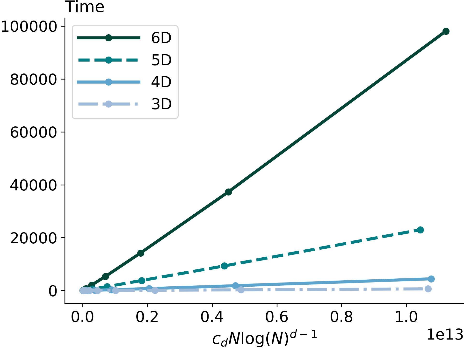
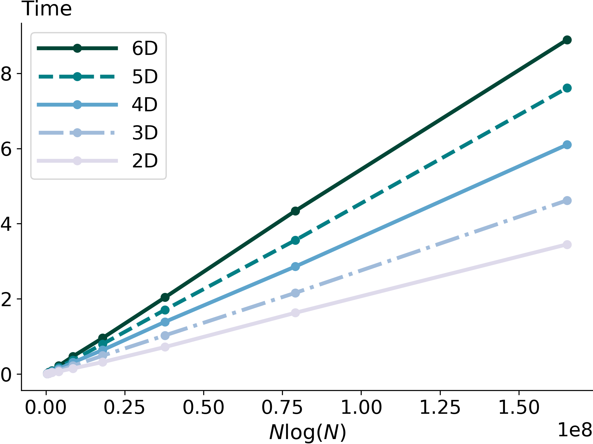
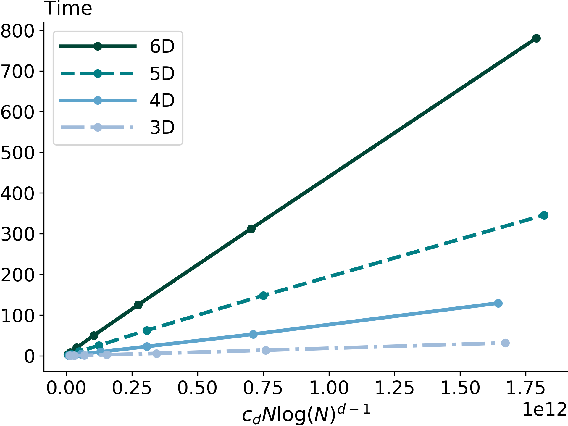
Figure 2 reports time calculation as a function of $N{\log}N$ for the fast summation approach and as a function of $c_{d}N\log(N)^{d-1}$ for the divide-and-conquer approach, with the scaling constants $c_{3}=3000$, $c_{4}=200$, $c_{5}=15$, $c_{6}=1$ chosen to make the visual comparison easier. The resulting straight lines confirm the theoretical complexity.

Figure 2: Runtime for CDF estimation (left: fast summation; right: divide-and-conquer)

The CDF values calculated by the naive approach and the two fast methods are exactly the same with no rounding error whatsoever since the $y{\equiv}1$ case is a counting problem (integer count values with final division by $N$; see Remark 2.1 on the fast summation case).
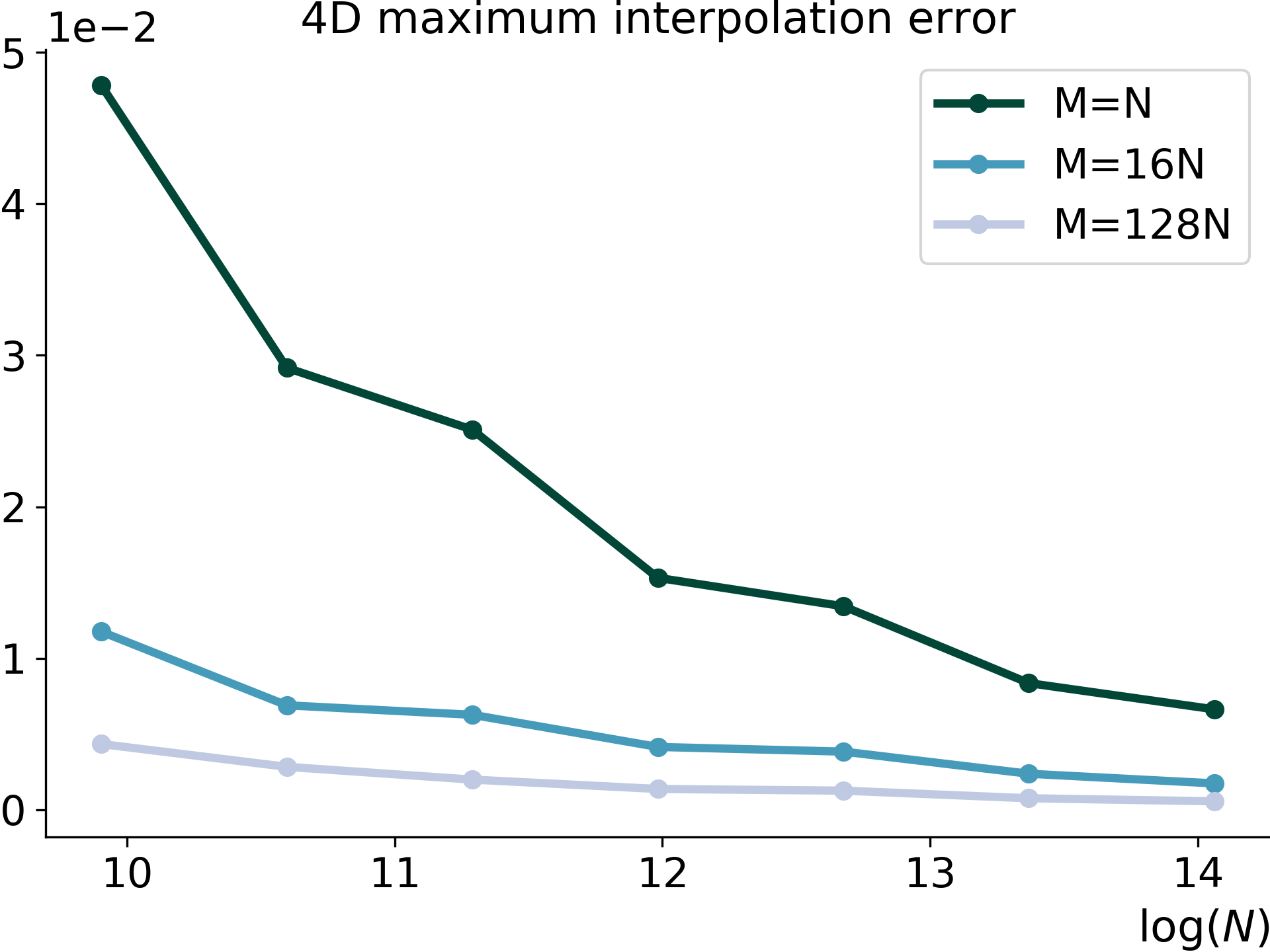
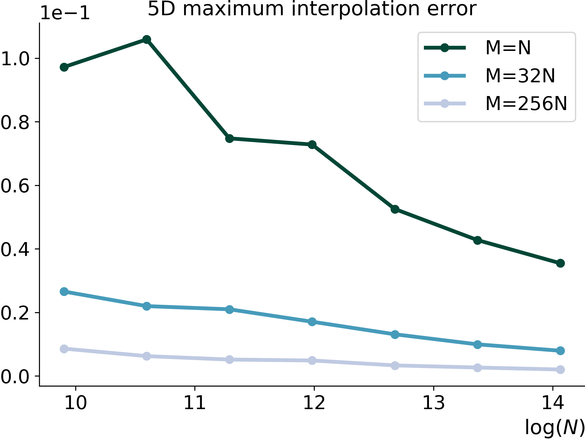
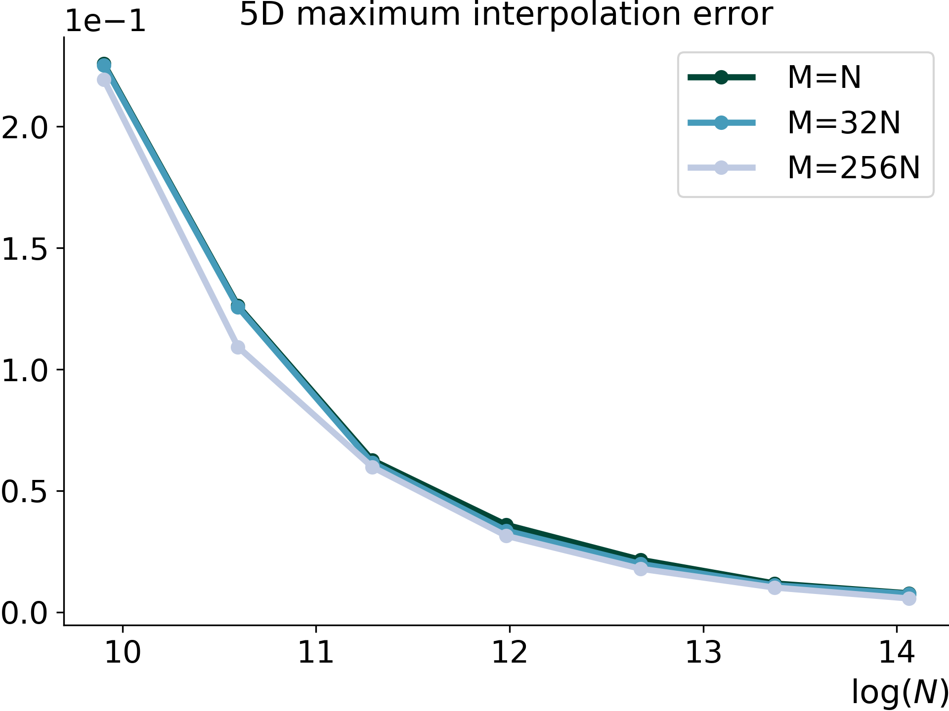
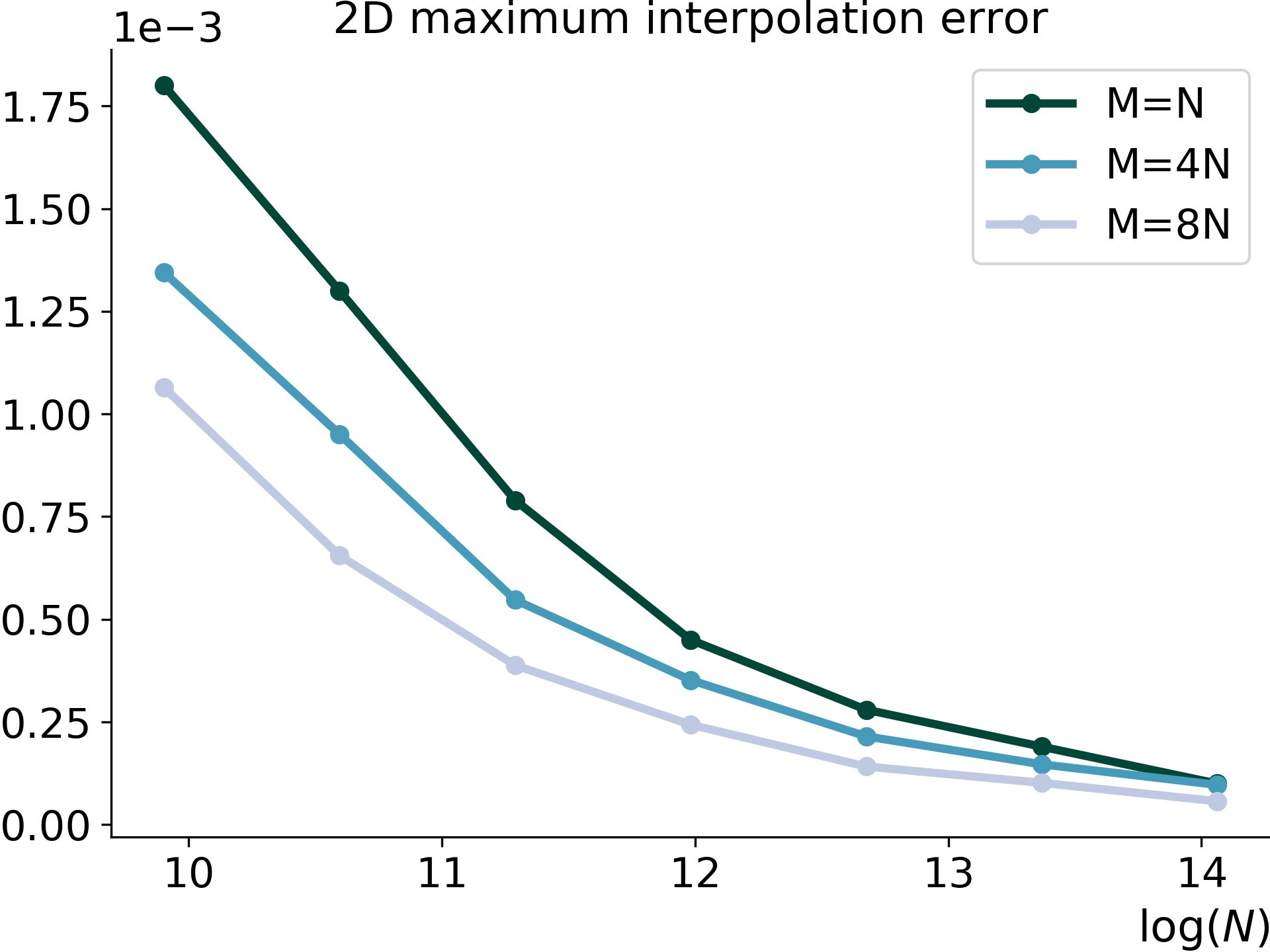
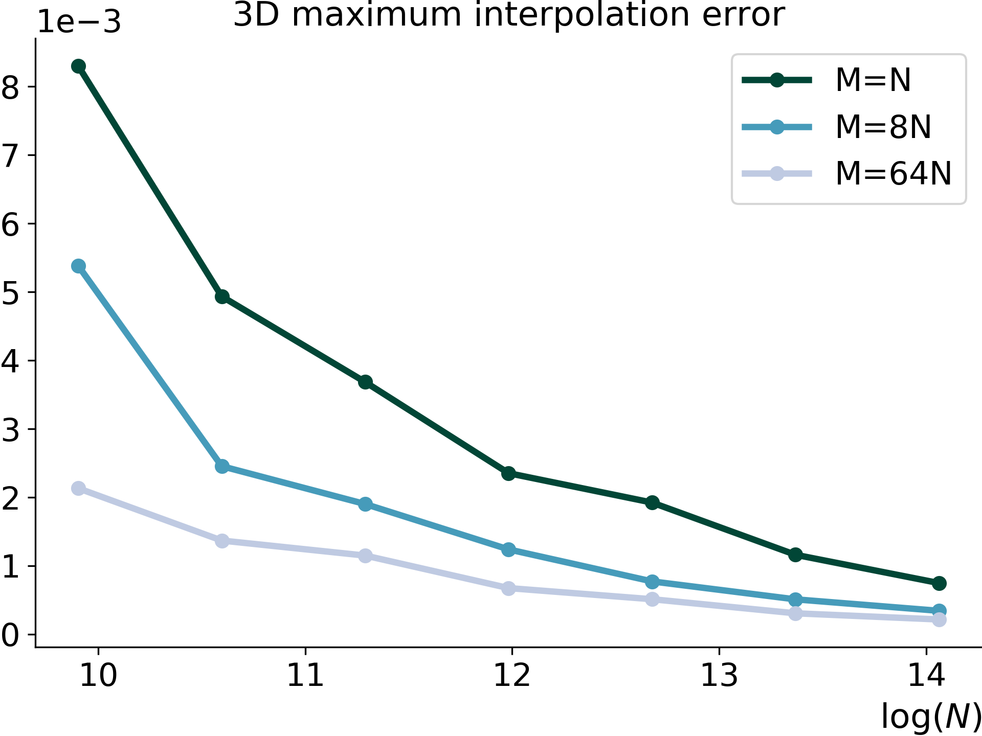
Suppose now that we specifically want to estimate the CDF values at the input points. The divide-and-conquer approach does this by design, while the fast summation approach requires an interpolation from the grid points to the input points. Figure 3 reports, for different numbers $M$ of evaluation points, the maximum interpolation error over the $N$ sample points between the CDF values computed by fast summation and linearly interpolated to the input points, and the divide-and-conquer CDF values (taken as reference).

Figure 3: Maximal error on CDF for evaluation at sample points using fast summation and interpolation taking as reference the divide and conquer calculation.

When $M=N$, one can see that the worst-case interpolation error ranges from around 1 ${\scriptstyle\mathsf{E}}$-4 for $d=2$ and $N=1,280,000$ to around 1 ${\scriptstyle\mathsf{E}}$-1 for $d=5$ and $N=20,000$. This worst-case interpolation error is lower for small $d$ and large $N$, and can be reduced by using a finer evaluation grid, i.e. taking $M$ larger than $N$, as shown by the three curves on Figure 3. Beyond linear interpolation, one could also resort to higher-order interpolation to reduce this error. Nevertheless, these results show that computing CDF values at input points by fast summation + interpolation is a viable method, with better results in the small $d$ high $N$ case.

4.2 Kernel density estimation

We now perform the same numerical tests for kernel density estimation, more specifically Laplacian kernel density estimation (equation (12)).
Table 3 reports KDE calculation time (in seconds) on a bivariate example with the naive, fast summation and divide-and-conquer approaches. Once again, the fast summation and divide-and-conquer methods offer a massive speedup compared to naive summation (respectively 0.34s and 2.29s vs. almost eight hours for the direct computation of (11) for 0,64 million points for example), and both fast computation times are of the same order, up to a constant factor (around $6.0$).

Nb particles	20,000	40,000	80,000	160,000	320,000	640,000
Fast summation time	0.01	0.01	0.04	0.08	0.14	0.34
Divide-and-conquer time	0.05	0.08	0.19	0.43	0.99	2.29
Naive time	28	115	439	1742	7198	28132

Table 3: 2D KDE calculation time (in seconds)

As in the CDF case, the computation time gap between the two fast methods grows with the dimension, as shown on Table 4.

Nb particles	20,000	40,000	80,000	160,000	320,000	640,000	1,280,000
Fast summation time	0.18	0.26	0.65	1.51	3.59	7.97	16.11
Divide-and-conquer time	15	41	111	294	777	2040	5344

Table 4: 6D KDE calculation time (in seconds)

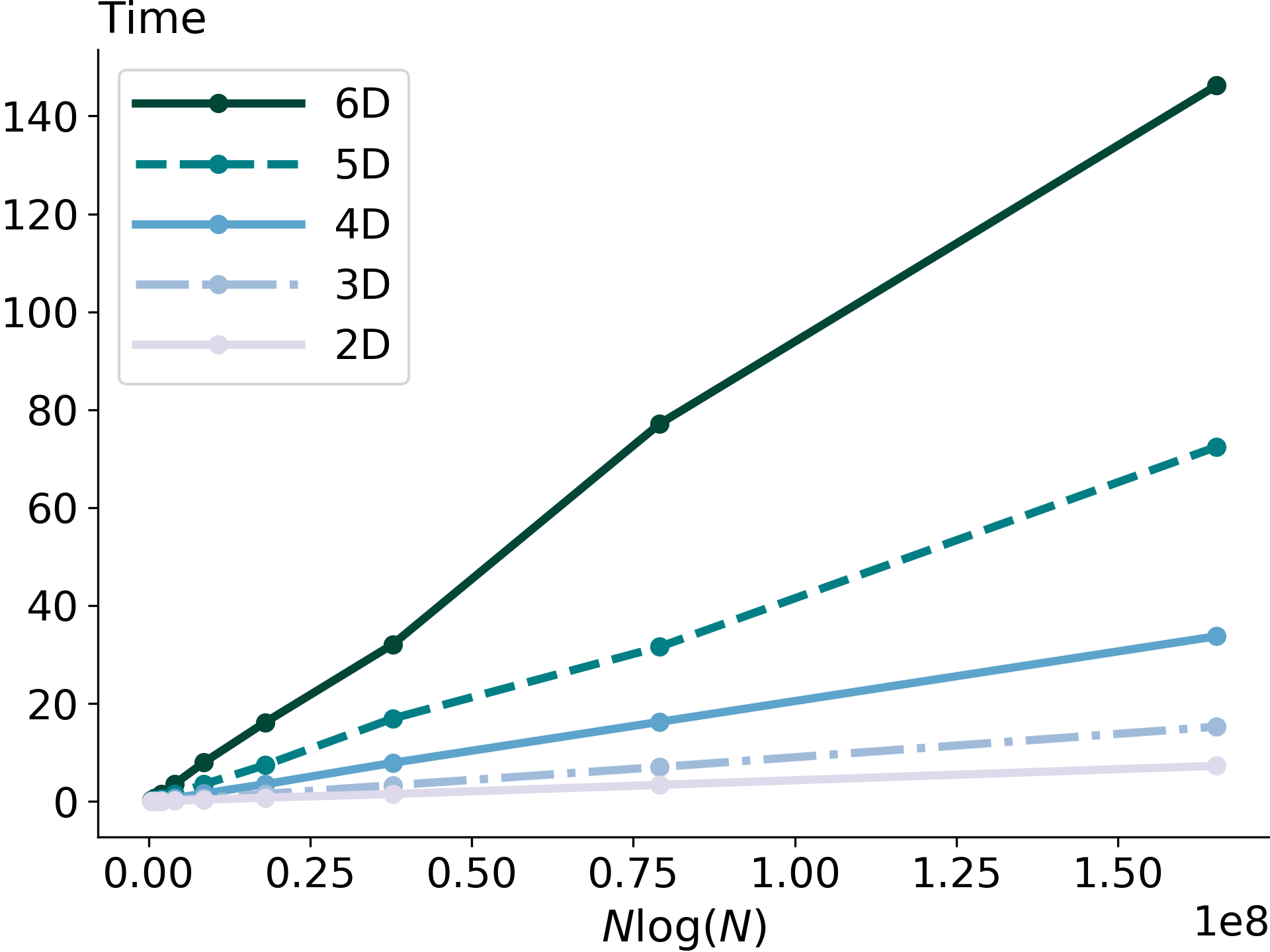
Figure 4 reports time calculation as a function of $N{\log}N$ for the fast summation approach and as a function of $c_{d}N\log(N)^{d-1}$ for the divide-and-conquer approach (with scaling constants $c_{3}=4000$, $c_{4}=250$, $c_{5}=20$, $c_{6}=1$). Once again, the resulting straight lines confirm the theoretical complexity.

Figure 4: Runtime for KDE estimation (left: fast summation; right: divide-and-conquer)

As for accuracy, the maximum difference between the KDE values of the naive approach and those of both fast methods, caused by float rounding errors, remains below 1 ${\scriptstyle\mathsf{E}}$-14 independently of the dimension of the problem.

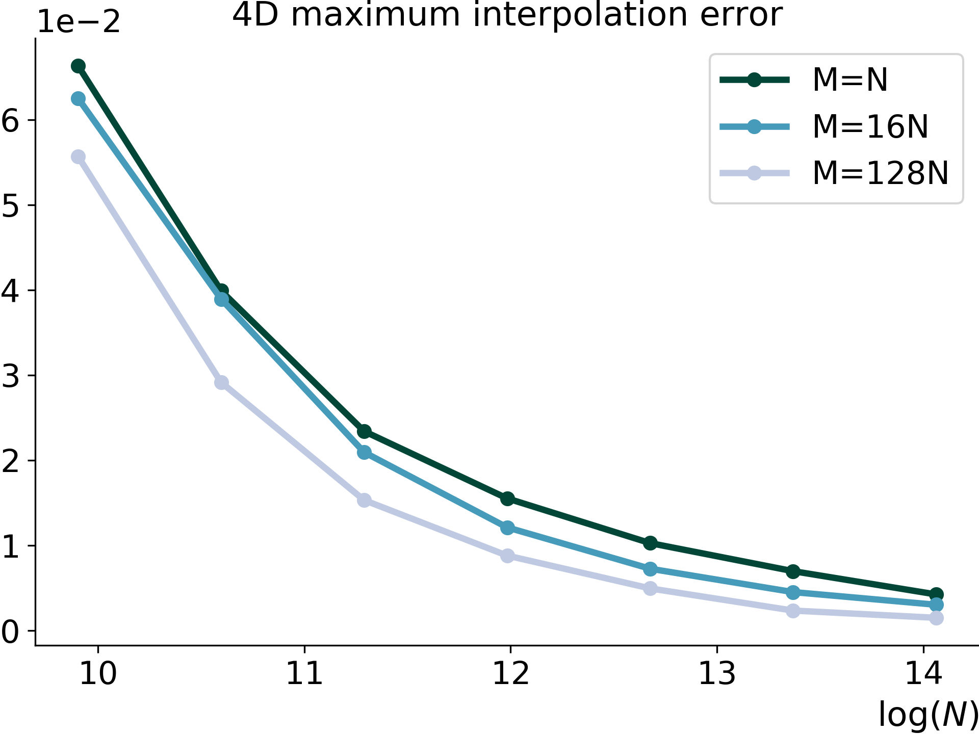
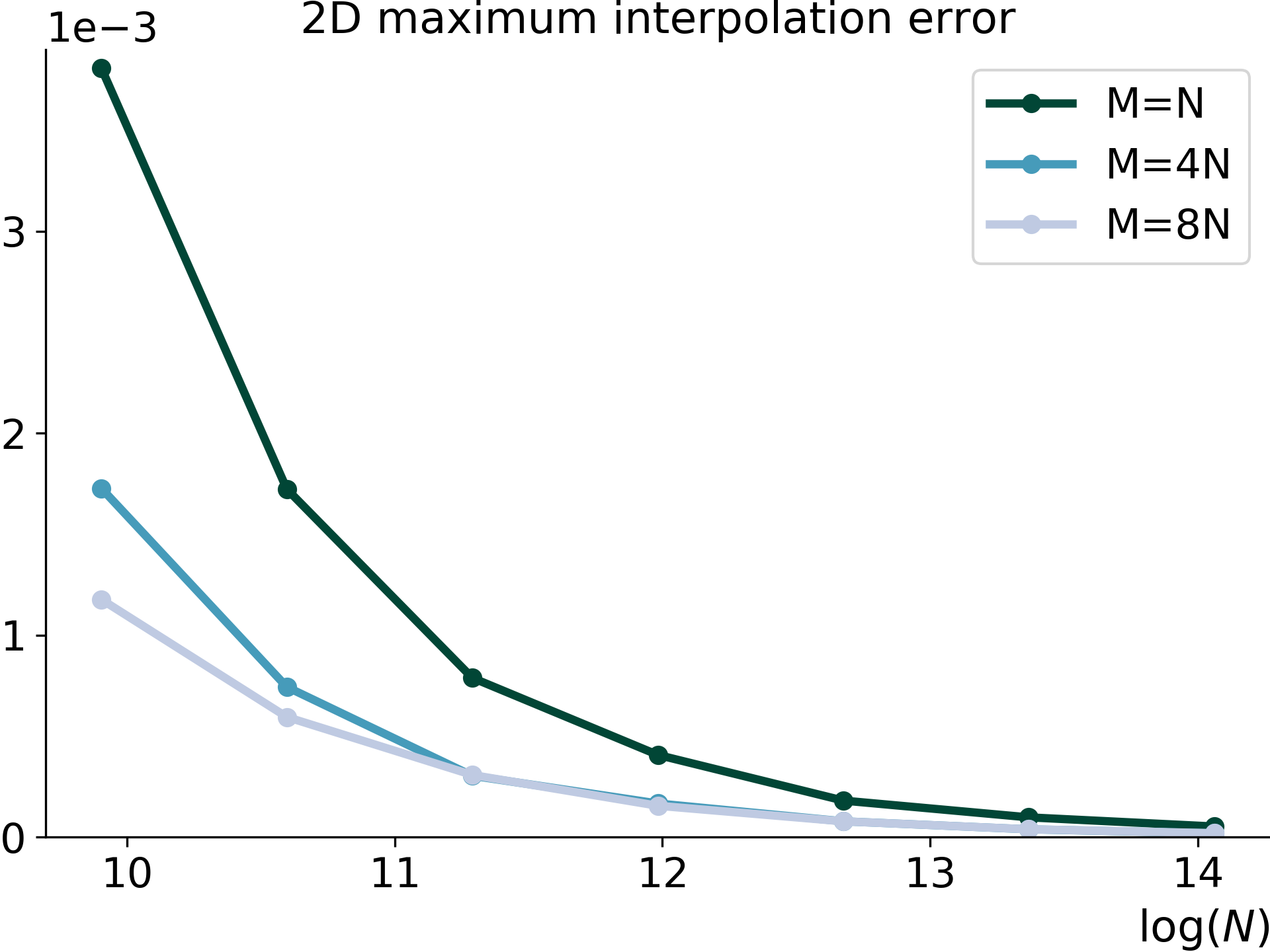
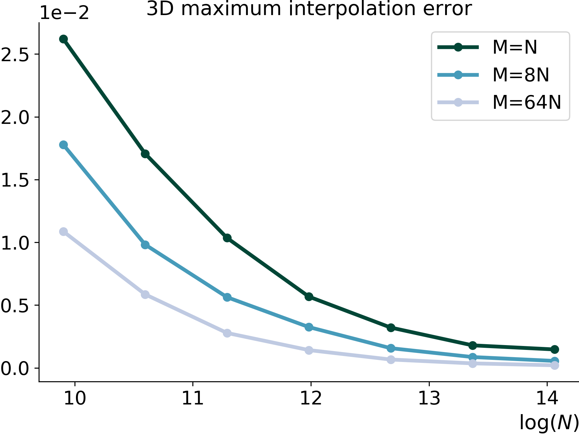
Finally, we also test the accuracy of the fast summation approach when the evaluation points are required to coincide with the input points, which requires an interpolation from the grid points. Figure 5 reports the maximum interpolation error over the $N$ sample points between the linearly interpolated CDF values computed by fast summation and the divide-and-conquer CDF values.

Figure 5: Maximal error on KDE evaluation at sample points using fast summation and interpolation taking as reference the divide and conquer calculation.

As in the CDF case, the worst-case interpolation error ranges between around 1 ${\scriptstyle\mathsf{E}}$-4 and 2 ${\scriptstyle\mathsf{E}}$-1, is smaller for small $d$, large $N$ or large $M$. However, the accuracy improvements obtained by increasing $M$ get smaller in higher dimension. Nevertheless, the fast summation + interpolation approach can still be considered a viable option for KDE estimation at the input data points, provided $d$ is small or $N$ is large.

5 Conclusion

A new algorithm based on fast summation in lexicographical order has been developed to efficiently calculate multivariate empirical cumulative distribution functions (ECDFs) with $O(N{\log}N)$ computational cost for $N$ arbitrary data points and $N$ evaluation points on a rectilinear grid. Numerical tests and comparisons to a state-of-the-art $\mathcal{O}(N\log(N)^{(d-1){\vee}1})$ divide-and-conquer algorithm confirm the speed of this exact algorithm.
Besides, we establish a multivariate decomposition formula of kernel density estimators (KDEs) into a weighted sum of generalized ECDFs for a large class of kernels. This connection leads to new fast KDE algorithms: one based on fast summation with $O(N{\log}N)$ complexity, and one based on divide-and-conquer recursion with $\mathcal{O}(N\log(N)^{(d-1){\vee}1})$ complexity.
The class of compatible kernels includes classical kernels such as the uniform, Epanechnikov and Laplacian kernels. We show that it also includes the Sargan and Matérn kernels, which can be used to approximate incompatible kernels such as the Gaussian kernel.
Following our computational breakthrough, several possible extensions and potential future work come to mind:

• The investigation of computational methods for the related kernel distribution estimation problem (Yamato 1973, Liu  Yang 2008) based on the algorithmic approaches developed in this paper.

• Further investigation of the promising class of multivariate polynomial-exponential kernels, in particular their ability to approximate multivariate kernels, and their ability to speed up statistical techniques based on multivariate Gaussian variables using the fast algorithms from this paper.

• The application of fast kernel regression for image processing, as uniform pixel grids are an ideal ground for Algorithm 1 for which its computational complexity is an optimal $\mathcal{O}(N)$.

• The comparison, more generally, of our algorithms to fast convolution methods such as the Fast Fourier Transform (FFT) for compatible convolution kernels.

Appendix A Computation of local sums

This appendix details how to efficiently compute the local sums $s_{j_{1},j_{2},\ldots,j_{d}}$ defined in equation (4) (subsection 2.1). Subsection A.1 details the general case, based on independent input data sorting in each dimension, for a $\mathcal{O}(N\log N)$ computational cost. Subsection A.2 details the uniform grid case: in this special case, the computational cost can be brought down to $\mathcal{O}(N)$ by using constant mesh divisions as a substitute to sorting.

A.1 General case

Input: input sample $x_{i}=(x_{1,i},\ldots,x_{d,i})$, $i=1,2,\ldots,N$

Input: evaluation grid $(z_{1,j_{1}},z_{2,j_{2}},\ldots,z_{d,j_{d}})$, $j_{k}\in\{1,2,\ldots,M_{k}\}$, $k\in\{1,2,\ldots,d\}$

Define index matrix $\mathrm{INDEX}[k,i]$

 $\triangleright$ local sum index $\in\{1,2,M_{k}+1\}$

where $k=1,2,\ldots,d$ and $i=1,2,\ldots,N$

for ${\color[rgb]{0.12109375,0.46484375,0.70703125}\mathbf{(}}$ $k=1,2,...\hskip 0.83298pt,d$ ${\color[rgb]{0.12109375,0.46484375,0.70703125}\mathbf{)}}$ do

      

      Sort the set $\left\{x_{k,1},\ldots x_{k,N}\right\}$ in increasing order, using for example quicksort or

      mergesort ($\mathcal{O}(N\log N)$): define the permutation $\phi_{k}:\{1,2,\ldots,N\}\mapsto\{1,2,\ldots,N\}$

      such that

$$x_{k,\phi_{k}(1)}<x_{k,\phi_{k}(2)}<\cdots<x_{k,\phi_{k}(N)}$$ (30)

      $x_{\mathrm{idx}}=1$

       $\triangleright$ input index $\in\{1,2,\ldots,N\}$

      

      $z_{\mathrm{idx}}=1$

       $\triangleright$ evaluation grid index $\in\{1,2,\ldots,M_{k}\}$

      

      while ${\color[rgb]{0.12109375,0.46484375,0.70703125}\mathbf{(}}$ $x_{\mathrm{idx}}\leq N$ ${\color[rgb]{0.12109375,0.46484375,0.70703125}\mathbf{)}}$ do

            

            if ${\color[rgb]{0.12109375,0.46484375,0.70703125}\mathbf{(}}$ $x_{k,\phi_{k}(x_{\mathrm{idx}})}\leq z_{k,z_{\mathrm{idx}}}$ ${\color[rgb]{0.12109375,0.46484375,0.70703125}\mathbf{)}}$ then

                  

                  $\mathrm{INDEX}[k,\phi_{k}(x_{\mathrm{idx}})]=z_{\mathrm{idx}}$

                  $x_{\mathrm{idx}}\,+\!=1$

            else

                  

                  $z_{\mathrm{idx}}\,+\!=1$

             end if

            

       end while

      

end for

$s_{j_{1},j_{2},\ldots,j_{d}}=0$, ${\scriptstyle\forall(j_{1},j_{2},\ldots,j_{d})\in\{1,2,\ldots,M_{1}+1\}\times\ldots\times\{1,2,\ldots,M_{d}+1\}}$

for ${\color[rgb]{0.12109375,0.46484375,0.70703125}\mathbf{(}}$ $i=1,2,...\hskip 0.83298pt,N$ ${\color[rgb]{0.12109375,0.46484375,0.70703125}\mathbf{)}}$ do

      

      $s_{\mathrm{INDEX}[1,i],\,\mathrm{INDEX}[2,i],\,\ldots,\,\mathrm{INDEX}[d,i]}\,+\!=y_{i}/N$

end for

Output: $s_{j_{1},j_{2},\ldots,j_{d}}=\frac{1}{N}\sum_{i=1}^{N}y_{i}\mathbbm{1}\{z_{1,j_{1}-1}<x_{1,i}\leq z_{1,j_{1}},\ldots,z_{d,j_{d}-1}<x_{d,i}\leq z_{d,j_{d}}\}$

               for every local sum index ${\scriptstyle(j_{1},j_{2},\ldots,j_{d})\in\{1,2,\ldots,M_{1}+1\}\times\ldots\times\{1,2,\ldots,M_{d}+1\}}$

Algorithm 6 Fast computation of local sums by independent sorting in each dimension

Algorithm 6 has a $\mathcal{O}(N{\log}N)$ computational complexity, owing to the data sorting in each dimension. Its memory complexity is $\mathcal{O}(N+M)$.

Remark A.1.

An alternative algorithm to compute the same local sums has been proposed in Bouchard  Warin (2012). It is based on partial sorts in each dimension and its computational complexity is $\mathcal{O}((\sum_{k=1}^{d}M_{k}+1)N)$. This complexity is better than $\mathcal{O}(N\log N)$ when $M{\ll}{\log}(N)^{d}$. However, in the case when $M{\approx}N$ (and $M_{1}=M_{2}=\ldots=M_{d}$), its equivalent $\mathcal{O}(N^{1+\frac{1}{d}})$ complexity does not improve over Algorithm 6.

A.2 Uniform grid case

Input: input sample $x_{i}=(x_{1,i},\ldots,x_{d,i})$, $i=1,2,\ldots,N$

Input: evaluation grid $(z_{1,j_{1}},z_{2,j_{2}},\ldots,z_{d,j_{d}})$, $j_{k}\in\{1,2,\ldots,M_{k}\}$, $k\in\{1,2,\ldots,d\}$

Define index matrix $\mathrm{INDEX}[k,i]$

 $\triangleright$ local sum index $\in\{1,2,M_{k}+1\}$

where $k=1,2,\ldots,d$ and $i=1,2,\ldots,N$

for ${\color[rgb]{0.12109375,0.46484375,0.70703125}\mathbf{(}}$ $k=1,2,...\hskip 0.83298pt,d$ ${\color[rgb]{0.12109375,0.46484375,0.70703125}\mathbf{)}}$ do

      

      $\Delta z_{k}\triangleq z_{k,2}-z_{k,1}$

       $\triangleright$ constant mesh $=z_{k,3}-z_{k,2}=z_{k,4}-z_{k,3}=\ldots$

      

      

      for ${\color[rgb]{0.12109375,0.46484375,0.70703125}\mathbf{(}}$ $i=1,2,...\hskip 0.83298pt,N$ ${\color[rgb]{0.12109375,0.46484375,0.70703125}\mathbf{)}}$ do

            

            

             $\triangleright$ mesh division rounded to upper integer

            

            $\mathrm{INDEX}[k,i]=\max(\,1\,,\,\min(\,M_{k}+1\,,\,1+\left\lceil(x_{k,i}-z_{k,1})/\Delta z_{k}\right\rceil\,)\,)$

       end for

      

end for

$s_{j_{1},j_{2},\ldots,j_{d}}=0$, ${\scriptstyle\forall(j_{1},j_{2},\ldots,j_{d})\in\{1,2,\ldots,M_{1}+1\}\times\ldots\times\{1,2,\ldots,M_{d}+1\}}$

for ${\color[rgb]{0.12109375,0.46484375,0.70703125}\mathbf{(}}$ $i=1,2,...\hskip 0.83298pt,N$ ${\color[rgb]{0.12109375,0.46484375,0.70703125}\mathbf{)}}$ do

      

      $s_{\mathrm{INDEX}[1,i],\,\mathrm{INDEX}[2,i],\,\ldots,\,\mathrm{INDEX}[d,i]}\,+\!=y_{i}/N$

end for

Output: $s_{j_{1},j_{2},\ldots,j_{d}}=\frac{1}{N}\sum_{i=1}^{N}y_{i}\mathbbm{1}\{z_{1,j_{1}-1}<x_{1,i}\leq z_{1,j_{1}},\ldots,z_{d,j_{d}-1}<x_{d,i}\leq z_{d,j_{d}}\}$

               for every local sum index ${\scriptstyle(j_{1},j_{2},\ldots,j_{d})\in\{1,2,\ldots,M_{1}+1\}\times\ldots\times\{1,2,\ldots,M_{d}+1\}}$

Algorithm 7 Fast computation of local sums by mesh division on uniform grid

Algorithm 7 has a $\mathcal{O}(N)$ computational complexity, and $\mathcal{O}(N+M)$ memory complexity.

Appendix B General matrix bandwidth

The general multivariate weighted Parzen-Rosenblatt kernel density estimator is defined by:

$$\hat{f}_{\mathrm{KDE}}(z)=\frac{1}{\left|H\right|^{1/2}N}\sum_{i=1}^{N}w_{i}K_{d}\!\left(H^{-1/2}(x_{i}-z)\right)$$ (31)

where $H$ is a symmetric positive definite $d\times d$ bandwidth matrix, see for example Wand  Jones (1995). As pointed out in Langrené  Warin (2019), one can without loss of generality focus on the diagonal bandwidth case $H=\mathrm{diag}(h)$, where $h=(h_{1},h_{2},\ldots,h_{d})\in\mathbb{R}^{d}$. Indeed, the eigenvalue decomposition of the symmetric positive definite matrix $H$ is given by $H=R\Delta^{2}R^{\top}$ where $R$ is a rotation matrix and $\Delta=\mathrm{diag}(h)$ is a diagonal matrix with strictly positive diagonal elements. Consequently, $H^{-1/2}(x_{i}-z)=\mathrm{diag}(\frac{1}{h})(R^{T}x_{i}-R^{T}z)$. By rotating both the input points $x_{i}$ and the evaluation point $z$ using the rotation matrix $R^{T}$, the multivariate kernel density estimator (31) becomes

$$\hat{f}_{\mathrm{KDE}}(z)=\frac{1}{N\Pi_{k=1}^{d}h_{k}}\sum_{i=1}^{N}w_{i}K_{d}\!\left(\frac{x_{i}-z}{h}\right)$$ (32)

where $x_{i}$ and $z$ denote respectively the input points and evaluation point in the new coordinates. In the Laplacian kernel case, equation (32) turns into the multivariate KDE equation (11) used in Section 3.

Appendix C Multivariate Matérn kernel

Taking the Matérn-3/2 kernel (25) ($p=1$) with $h=\sqrt{3}$ as example, several approaches exist to define a multivariate kernel. One approach, known as product kernel, is to multiply univariate kernels:

$$K_{d}(u)=\frac{1}{4^{d}}\prod_{k=1}^{d}\left(1+\left|u_{k}\right|\right)e^{-\left|u_{k}\right|}$$ (33)

Another approach is to replace the absolute value $\left|u\right|$ by the L1 norm $\left\|u\right\|_{1}=\sum_{k=1}^{d}\left|u_{k}\right|$, along with a correction of the normalization constant:

$$K_{d}(u)=\frac{1}{2^{d}(1+d)}\left(1+\sum_{k=1}^{d}\left|u_{k}\right|\right)e^{-\sum_{k=1}^{d}\left|u_{k}\right|}$$ (34)

The product approach (33) preserves the continuous differentiability of the kernel, which is not the case for the additive approach (34). Nevertheless, the CDF decomposition of the additive kernel (34) contains significantly fewer terms than the one of the product kernel (33). Indeed, the KDE decomposition of (34) is given by

$$\frac{1}{N\prod_{k=1}^{d}h_{k}}\sum_{i=1}^{N}w_{i}K_{d}\left(\frac{x_{i}-z}{h}\right)$$

$$= \frac{1}{2^{d}(1+d)}\frac{1}{N\prod_{k=1}^{d}h_{k}}\sum_{i=1}^{N}w_{i}\left(1+\sum_{l=1}^{d}\left|\frac{x_{l,i}-z_{l}}{h_{l}}\right|\right)e^{-\sum_{k=1}^{d}\left|\frac{x_{k,i}-z_{k}}{h_{k}}\right|}$$

$$= \frac{1}{2^{d}(1+d)}\frac{1}{N\prod_{k=1}^{d}h_{k}}\sum_{i=1}^{N}w_{i}\left(1+\sum_{l=1}^{d}\left|\frac{x_{l,i}-z_{l}}{h_{l}}\right|\right)$$

$$\left.\times\prod_{k=1}^{d}\left(e^{-\frac{z_{k}}{h_{k}}}e^{\frac{x_{k,i}}{h_{k}}}\mathbbm{1}\{x_{k,i}\leq z_{k}\}+e^{\frac{z_{k}}{h_{k}}}e^{-\frac{x_{k,i}}{h_{k}}}\mathbbm{1}\{-x_{k,i}<-z_{k}\}\right)\right)$$

$$= \frac{1}{2^{d}(1+d)}\frac{1}{N\prod_{k=1}^{d}h_{k}}\sum_{i=1}^{N}\sum_{\delta\in\{-1,1\}^{d}}e^{-\sum_{k=1}^{d}\frac{\delta_{k}z_{k}}{h_{k}}}\left(1+\sum_{l=1}^{d}\left|\frac{x_{l,i}-z_{l}}{h_{l}}\right|\right)$$

$$\left.\times w_{i}e^{\sum_{k=1}^{d}\frac{\delta_{k}x_{k,i}}{h_{k}}}\mathbbm{1}\{\delta_{1}x_{1,i}\leq_{\delta_{1}}\delta_{1}z_{1},\ldots,\delta_{d}x_{d,i}\leq_{\delta_{d}}\delta_{d}z_{d}\}\right)$$

$$= \frac{1}{2^{d}(1+d)}\frac{1}{N\prod_{k=1}^{d}h_{k}}\sum_{i=1}^{N}\sum_{\delta\in\{-1,1\}^{d}}e^{-\sum_{k=1}^{d}\frac{\delta_{k}z_{k}}{h_{k}}}\left(1-\sum_{l=1}^{d}\delta_{l}\frac{x_{l,i}-z_{l}}{h_{l}}\right)$$

$$\left.\times w_{i}e^{\sum_{k=1}^{d}\frac{\delta_{k}x_{k,i}}{h_{k}}}\mathbbm{1}\{\delta_{1}x_{1,i}\leq_{\delta_{1}}\delta_{1}z_{1},\ldots,\delta_{d}x_{d,i}\leq_{\delta_{d}}\delta_{d}z_{d}\}\right)$$

$$= \frac{1}{2^{d}(1+d)}\frac{1}{\prod_{k=1}^{d}h_{k}}\sum_{\delta\in\{-1,1\}^{d}}e^{-\sum_{k=1}^{d}\frac{\delta_{k}z_{k}}{h_{k}}}\left(\left(1+\sum_{l=1}^{d}\frac{\delta_{l}z_{l}}{h_{l}}\right)F_{N}(\delta z,\delta;\delta x,y^{(0)})-\sum_{l=1}^{d}\frac{\delta_{l}}{h_{l}}F_{N}(\delta z,\delta;\delta x,y^{(l)})\right)$$ (35)

with $y_{i}^{(0)}=y_{i}^{(0)}(\delta)\triangleq w_{i}e^{\sum_{k=1}^{d}\frac{\delta_{k}x_{k,i}}{h_{k}}}$ and $y_{i}^{(l)}=y_{i}^{(l)}(\delta)\triangleq w_{i}x_{l,i}e^{\sum_{k=1}^{d}\frac{\delta_{k}x_{k,i}}{h_{k}}}$. This decomposition contains $2^{d}(d+1)$ CDFs to compute. By contrast, similar computations show that the KDE decomposition of the product kernel (33) contains a total of $4^{d}$ CDFs to compute. In other words, the additive kernel (34) is much more attractive than the product kernel (33) from a computational point of view, even when accounting for its lower efficiency. These two kernels are however not as computationally attractive as the Laplacian and uniform kernels, whose CDF decompositions contain $2^{d}$ terms ((12) and (18)).

Appendix D Divide-and-conquer for Laplacian kernel density estimation

This Appendix explains how to adapt the divide-and-conquer algorithm described in Section 2.2 to compute the $2^{d}$ CDF vectors $\{F_{N}(x_{i},\delta)\}_{i=1,N}$ required to compute equation (12). A possible approach would consist in adapting the algorithm 2 used to calculate (3) with $\delta=(1,..,1)$ by applying a modified version $2^{d}$ times to calculate the different terms.
We propose a single algorithm, implemented in the StOpt library, which makes it possible to compute the $F_{N}$ for all the $\delta$ in one recursion, avoiding to sort the particles $2^{d}$ times.
We give the algorithm obtained in general dimension to calculate for all $\delta\in\{-1,1\}^{d}$, and given $m$, $l$ with values in $1,\dots,d$, $(p,q)\in\mathds{N}^{2}$ a general term for $j=1,N$

$$\sum_{i=1}^{N}x_{l,i}^{p}x_{m,i}^{q}e^{\sum_{k=1}^{d}\frac{\delta_{k}x_{k,i}}{h_{k}}}\mathbbm{1}\{\delta_{1}x_{1,i}<\delta_{1}x_{1,j},\ldots,\delta_{d}x_{d,i}<\delta_{d}x_{d,j}\}.$$

Once again observe that the inequalities are strict in the expression above. As before the tests for non-empty sets are dropped out.

• Algorithm 8 is the main calling similar to 2. The special 2D case is dealt with the call of the two different one-dimensional merge algorithm 11 and 12 instead of a single one-dimensional algorithm.

• The $n$-dimensional merge algorithm 10 is similar to Algorithm 4. Besides, a set $\Delta$ of $\delta\in\{-1,1\}^{d}$ is given as input too such that either $\delta_{k}x_{k}\leq\delta_{k}y_{k}$ for $k>I_{dim}$ for all $x\in\kappa_{1}$ and $y\in\kappa_{2}$ or $\delta_{k}x_{k}>\delta_{k}y_{k}$ for $k>I_{dim}$ for all $x\in\kappa_{1}$ and $y\in\kappa_{2}$.
  For the couple of sets $(\kappa_{1,1},\kappa_{2,2})$,$(\kappa_{2,1},\kappa_{1,2})$ where dominance is clear in the current dimension, the $n$-dimensional merge algorithm is called in the dimension below and some subset of $\Delta$. In the case when $I_{dim}=2$, a direct call to the one-dimensional merge algorithms 11 and 12 is performed.

• Two one-dimensional merge in dimension 1 are used. The first version $\mathbf{Merge1D1}$ is used for the $\delta$ such that $\delta_{1}=1$ and is the same as the $\mathbf{Merge1D}$ algorithm except that it works for a set of $\delta$ given as input. The second one is for the $\delta$ such that $\delta_{1}=-1$.

Input: $x=(x_{i},\dots,x_{N})$, $\psi(x_{i},\delta)=x_{l,i}^{p}x_{m,i}^{q}e^{-\sum_{k=1}^{d}\frac{\delta_{k}x_{k,i}}{h_{k}}}$, for all $i=1,\dots,N$, $\delta\in\{-1,1\}^{d}$

Calculate $\phi^{j}$ , $j=1,\dots,d$ such that $x_{j,\phi^{j}(1)}\leq x_{j,\phi^{j}(2)}\leq\dots\leq x_{j,\phi^{j}(N)}$

$F(x_{i},\delta)=0$ for $i=1,\dots,N$, for all $\delta\in\{-1,1\}^{d}$

$\mathbf{RecurSplitting}(x,\psi,\phi,F,N)$

Output: $F(x_{i},\delta)$ for all $i\in[1,N]$ and all $\delta\in\{-1,1\}^{d}$

Algorithm 8 Calculate for $1\leq l\leq m\leq d$, $p$, $q$ given

$$F(x_{j},\delta)=\sum_{i=1}^{N}x_{l,i}^{p}x_{m,i}^{q}e^{\sum_{k=1}^{d}\frac{\delta_{k}x_{k,i}}{h_{k}}}\mathbbm{1}\{\delta_{1}x_{1,i}<\delta_{1}x_{1,j},\ldots,\delta_{d}x_{d,i}<\delta_{d}x_{d,j}\},\quad j=1,N,\delta\in\{-1,1\}^{d}$$

Input: $x$, $\psi$, $F$, $\phi^{j}(i)$ for $i=1,M$, $j=1,d$

$\kappa_{1}=\{\phi^{d}(i),i=1,\frac{M}{2}\}$, $\phi_{1}$ with values in $\kappa_{1}$ s.t. $x_{j,\phi_{1}^{j}(1)}\leq x_{j,\phi_{1}^{j}(2)}\leq\dots\leq x_{j,\phi_{1}^{j}(\frac{M}{2})}$, $j=1,d$

$\kappa_{2}=\{\phi^{d}(i),i=\frac{M}{2}+1,M\}$, $\phi_{2}$ in $\kappa_{2}$ s.t. $x_{j,\phi_{2}^{j}(1)}\leq x_{j,\phi_{2}^{j}(2)}\leq\dots\leq x_{j,\phi_{2}^{j}(\frac{M}{2})}$,$j=1,d$

$\mathbf{RecurSplitting}(x,\psi,\phi_{1},F,M/2)$

$\mathbf{RecurSplitting}(x,\psi,\phi_{2},F,M/2)$

if ${\color[rgb]{0.12109375,0.46484375,0.70703125}\mathbf{(}}$ d > 2 ${\color[rgb]{0.12109375,0.46484375,0.70703125}\mathbf{)}}$ then

       $\Delta=\{\delta\in\{-1,1\}^{d}\}$

       $\mathbf{MergeND}(x,\phi_{1},\phi_{2},d-1,\psi,F,M/2,M/2,\Delta)$

else

      

       $\triangleright$ Merge for all $\delta$

       $\mathbf{Merge1D1}(x,\phi_{1}^{1},\phi_{2}^{1},\psi,F,\hat{\Delta},M/2,M/2)$, with $\hat{\Delta}=\{(1,1)\}$

       $\mathbf{Merge1D2}(x,\phi_{1}^{1},\phi_{2}^{1},\psi,F,\hat{\Delta},M/2,M/2)$ with $\hat{\Delta}=\{(-1,1)\}$

       $\mathbf{Merge1D1}(x,\phi_{2}^{1},\phi_{1}^{1},\psi,F,\hat{\Delta},M/2,M/2)$ with $\hat{\Delta}=\{(1,-1)\}$

       $\mathbf{Merge1D2}(x,\phi_{2}^{1},\phi_{1}^{1},\psi,F,\hat{\Delta},M/2,M/2)$ with $\hat{\Delta}=\{(-1,-1)\}$

      

end if

Output: $F$ updated

Algorithm 9 Recursive splitting function $\mathbf{RecurSplitting}$

Input: $x$, $\psi$, $F$, $\Delta\subset\{\delta\in\{-1,1\}^{d}\}$ , $\phi_{1}^{j}(i)$, for all $i=1,M_{1}$, $\phi_{2}^{j}(i)$, for all $i=1,M_{2}$ with values in $[1,N]$ for $j=1,I_{dim}$

 $\triangleright$ $\delta\in\Delta$ s.t. $\delta_{k}x_{k}\leq\delta_{k}y_{k}$ for $k>I_{dim}$ for all $x\in\kappa_{1}$ and $y\in\kappa_{2}$ or $\delta_{k}x_{k}>\delta_{k}y_{k}$ for $k>I_{dim}$ for all $x\in\kappa_{1}$ and $y\in\kappa_{2}$

$\kappa_{1}=\{\phi_{1}^{I_{dim}}(i),i=1,M_{1}\}$ , $\kappa_{2}=\{\phi_{2}^{I_{dim}}(i),i=1,M_{2}\}$

$\kappa=\kappa_{1}\cup\kappa_{2}$, $x_{med}$ s.t; $\#\{x_{j},j\in\kappa,x_{I_{dim},j}\leq x_{med}\}=\#\{x_{j},j\in\kappa,x_{I_{dim},j}>x_{med}\}$

$\kappa_{l,1}=\{i\in\kappa_{l},x_{I_{dim},i}\leq x_{med}\}$, $M_{l,1}=\#\kappa_{l,1}$, for $l=1,2$,

$\kappa_{l,2}=\{i\in\kappa_{l},x_{I_{dim},i}>x_{med}\}$, $M_{l,2}=\#\kappa_{l,2}$, for $l=1,2$

Create $\phi_{l,m}^{j}(i)$, $i=1,\dots M_{l,m}$ s.t. $\phi_{l,m}^{j}(i)\in\kappa_{l,m}$, and

$$x_{j,\phi_{l,m}^{j}(1)}\leq x_{j,\phi_{l,m}^{j}(2)}\leq\dots\leq x_{j,\phi_{l,m}^{j}(M_{l,m})},\mbox{ for }j\leq I_{dim},\quad l=1,2,\quad m=1,2.$$

$\mathbf{MergeND}(x,\phi_{1,l},\phi_{2,l},I_{dim},\psi,F,M_{1,l},M_{2,l},\Delta)$, for $l=1,2$

if ${\color[rgb]{0.12109375,0.46484375,0.70703125}\mathbf{(}}$ $I_{dim}==2$ ${\color[rgb]{0.12109375,0.46484375,0.70703125}\mathbf{)}}$ then

      

       $\triangleright$ Merge the set of 3D problem directly without recursion

       $\mathbf{Merge1D1}(x,\phi_{1,1}^{1},\phi_{2,2}^{1},\psi,F,\hat{\Delta},M_{1,1},M_{2,2})$ so that $\hat{\Delta}=\{(1,1,1,..)\in\Delta\}$

       $\mathbf{Merge1D2}(x,\phi_{1,1}^{1},\phi_{2,2}^{1},\psi,F,\hat{\Delta},M_{1,1},M_{2,2})$ so that $\hat{\Delta}=\{(-1,1,1,\dots)\in\Delta\}$

       $\mathbf{Merge1D1}(x,\phi_{2,2}^{1},\phi_{1,1}^{1},\psi,F,\hat{\Delta},M_{2,2},M_{1,1})$ so that $\hat{\Delta}=\{(1,-1,-1,\dots)\in\Delta\}$

       $\mathbf{Merge1D2}(x,\phi_{2,2}^{1},\phi_{1,1}^{1},\psi,F,\hat{\Delta},M_{2,2},M_{1,1})$ so that $\hat{\Delta}=\{(-1,-1,-1,\dots)\in\Delta\}$

       $\mathbf{Merge1D1}(x,\phi_{1,2}^{1},\phi_{2,1}^{1},\psi,F,\hat{\Delta},M_{1,2},M_{2,1})$ so that $\hat{\Delta}=\{(1,-1,1,\dots)\in\Delta\}$

       $\mathbf{Merge1D2}(x,\phi_{1,2}^{1},\phi_{2,1}^{1},\psi,F,\hat{\Delta},M_{1,2},M_{2,1})$ so that $\hat{\Delta}=\{(-1,-1,1,\dots)\in\Delta\}$

       $\mathbf{Merge1D1}(x,\phi_{2,1}^{1},\phi_{1,2}^{1},\psi,F,\hat{\Delta},M_{2,1},M_{1,2})$ so that $\hat{\Delta}=\{(1,1,-1,\dots)\in\Delta\}$

       $\mathbf{Merge1D2}(x,\phi_{2,1}^{1},\phi_{1,2}^{1},\psi,F,\hat{\Delta},M_{2,1},M_{1,2})$ so that $\hat{\Delta}=\{-1,1,-1,\dots\}\in\Delta\}$

      

else

      

       $\triangleright$ Merge in dimension below

       $\mathbf{mergedND}(x,\phi_{1,1},\phi_{2,2},I_{dim}-1,\psi,F,M_{1,l},M_{2,l},\hat{\Delta})$, $\hat{\Delta}=\{\delta\in\Delta\mbox{ with },\delta_{I_{dim}}\delta_{I_{dim}+1}>0\}$

       $\mathbf{mergedND}(x,\phi_{2,1},\phi_{1,2},I_{dim}-1,\psi,F,M_{1,l},M_{2,l},\hat{\Delta})$, $\hat{\Delta}=\{\delta\in\Delta\mbox{ with },\delta_{I_{dim}}\delta_{I_{dim}+1}<0\}$

end if

Output: $F$ updated

Algorithm 10 Recursive merge nD $\mathbf{MergeND}$ in given dimension $I_{dim}$

Input: $x$, $\psi$, $F$, $\phi_{k}$ s.t. $\phi_{k}(i)\leq\phi_{k}(i+1)$, for all $i=1,M_{k}-1$, $k=1,2$, $\Delta\subset\{\delta\in\{-1,1\}^{d}\}$

$S(\delta)=0$ for all $\delta\in\Delta$, $j=0$

for ${\color[rgb]{0.12109375,0.46484375,0.70703125}\mathbf{(}}$ $i=1,M_{2}$ ${\color[rgb]{0.12109375,0.46484375,0.70703125}\mathbf{)}}$ do

       while ${\color[rgb]{0.12109375,0.46484375,0.70703125}\mathbf{(}}$ $(x_{\phi_{2}(i),1}\geq x_{\phi_{1}(j),1})$ and $j\leq M_{1}$ ${\color[rgb]{0.12109375,0.46484375,0.70703125}\mathbf{)}}$ do

             $S(\delta)+=\psi(\phi_{1}(j),\delta)$ for all $\delta\in\Delta$ , $j=j+1$

       end while

      $F(\phi_{2}(i),\delta)+=S(\delta)$ for all $\delta\in\Delta$

       if ${\color[rgb]{0.12109375,0.46484375,0.70703125}\mathbf{(}}$ $j==M_{1}+1$ ${\color[rgb]{0.12109375,0.46484375,0.70703125}\mathbf{)}}$ then

             for ${\color[rgb]{0.12109375,0.46484375,0.70703125}\mathbf{(}}$ $k=i+1,M_{2}$ ${\color[rgb]{0.12109375,0.46484375,0.70703125}\mathbf{)}}$ do

                   $F(\phi_{2}(k),\delta)+=S(\delta)$ for all $\delta\in\Delta$

             end for

            $i=M_{2}+1$

       end if

      

end for

Output: $F$ updated

Algorithm 11 Final merge function in dimension one : $\mathbf{Merge1D1}$ for two sets of points $\kappa_{1}=\{x_{\phi_{1}(i)},i=1,M_{1}\}$, $\kappa_{2}=\{x_{\phi_{2}(i)},i=1,M_{2}\}$ such that for $x\in\kappa_{1}$, $y\in\kappa_{2}$, $\delta_{k}x_{k}\leq\delta_{k}y_{k}$ for $k\in[2,d]$, for all $\delta\in\Delta$. All elements $\delta$ of $\Delta$ are such that $\delta_{1}=1$.

Input: $x$, $\psi$, $F$, $\phi_{k}$ s.t. $\phi_{k}(i)\leq\phi_{k}(i+1)$, for all $i=1,M_{k}-1$, $k=1,2$, $\Delta\subset\{\delta\in\{-1,1\}^{d}\}$

$S(\delta)=0$ for all $\delta\in\Delta$, $j=M_{1}$

for ${\color[rgb]{0.12109375,0.46484375,0.70703125}\mathbf{(}}$ $i=M_{2},1$ ${\color[rgb]{0.12109375,0.46484375,0.70703125}\mathbf{)}}$ do

       while ${\color[rgb]{0.12109375,0.46484375,0.70703125}\mathbf{(}}$ $(x_{\phi_{2}(i),1}<x_{\phi_{1}(j),1})$ and $j\geq 1$ ${\color[rgb]{0.12109375,0.46484375,0.70703125}\mathbf{)}}$ do

             $S(\delta)+=\psi(\phi_{1}(j),\delta)$ for all $\delta\in\Delta$ , $j=j-1$

       end while

      $F(\phi_{2}(i),\delta)+=S(\delta)$ for all $\delta\in\Delta$

       if ${\color[rgb]{0.12109375,0.46484375,0.70703125}\mathbf{(}}$ $j==0$ ${\color[rgb]{0.12109375,0.46484375,0.70703125}\mathbf{)}}$ then

             for ${\color[rgb]{0.12109375,0.46484375,0.70703125}\mathbf{(}}$ $k=1,i-1$ ${\color[rgb]{0.12109375,0.46484375,0.70703125}\mathbf{)}}$ do

                   $F(\phi_{2}(k),\delta)+=S(\delta)$ for all $\delta\in\Delta$

             end for

            $i=0$

       end if

      

end for

Output: $F$ updated

Algorithm 12 Final merge function in dimension one : $\mathbf{Merge1D2}$ for two sets of points $\kappa_{1}=\{x_{\phi_{1}(i)},i=1,M_{1}\}$, $\kappa_{2}=\{x_{\phi_{2}(i)},i=1,M_{2}\}$ such that for $x\in\kappa_{1}$, $y\in\kappa_{2}$, $\delta_{k}x_{k}\leq\delta_{k}y_{k}$ for $k\in[2,d]$, for all $\delta\in\Delta$. All elements $\delta$ of $\Delta$ are such that $\delta_{1}=-1$.