Superfluidity of dipolar magnetoexcitons in doped double-layered $\alpha$-${\cal T}_{3}$ lattice in a strong magnetic field

Abstract

We predict the occurrence of Bose-Einstein condensation and superfluidity of dipolar magnetoexcitons for a pair of quasi-two-dimensional spatially separated $\alpha$-${\cal T}_{3}$ layers. We have solved a two-body problem for an electron and a hole for the model Hamiltonian for the $\alpha$-${\cal T}_{3}$ double layer in a magnetic field. The energy dispersion of collective excitations, the spectrum of sound velocity, and the effective magnetic mass of magnetoexcitons are obtained in the integer quantum Hall regime for high magnetic fields. The superfluid density and the temperature of the Kosterlitz-Thouless phase transition are probed as functions of the excitonic density, magnetic field and the inter-layer separation.

I Introduction

The many-particle systems of dipolar (indirect) excitons, formed by spatially separated electrons and holes, in semiconductor coupled quantum wells (CQWs) in a magnetic field $B$, as well as in the absence of magnetic field, have attracted considerable attention. This interest has been generated in large part by the possibility of Bose-Einstein condensation (BEC) and superfluidity of dipolar excitons, which can be observed as persistent electrical currents in each quantum well, and also through coherent optical properties Lozovik ; Snoke ; Butov ; Eisenstein . Recent progress in theoretical and experimental studies of the superfluidity of dipolar excitons in CQWs was reviewed in Ref. Snoke_review .

Recently, a number of experimental and theoretical studies were dedicated to graphene, and the condensation of electron-hole pairs, formed by spatially separated electrons and holes, in a pair of parallel graphene layers. These investigations were reported in Refs. BLG ; Sokolik ; Bist ; BKZg ; Perali . Since the exciton binding energies in novel two-dimensional (2D) semiconductors is quite large, both BEC and superfluidity of dipolar excitons in double layers of transition-metal dichalcogenides (TMDCs) Fogler ; MacDonald_TMDC ; BK ; BK2 and phosphorene BGK ; Peeters have been discussed. In high magnetic fields, 2D excitons referred to as magnetoexcitons exist in a much wider temperature range, since the magnetoexciton binding energies increase as the magnetic field is increased  Lerner ; Paquet ; Kallin ; Yoshioka ; Ruvinsky ; Ulloa ; Moskalenko .

Lately, there has been growing interest in the electronic properties of the $\alpha$-${\cal T}_{3}$ lattice for its surprising fundamental physical phenomena as well as its promising applications in solid state devicesf1 ; f2 ; f3 ; f4 ; f5 ; f6 ; f7 ; f8 ; f9 ; RKKY ; t1 ; t2 ; t3 . For a review of artificial flat band systems, see Ref.  Review . Raoux, et al. f1 proposed that an $\alpha$-${\cal T}_{3}$ lattice could be assembled from cold fermionic atoms confined to an optical lattice by means of three pairs of laser beams for the optical dice lattice ($\alpha=1$) 21 . A model of this structure, consists of an AB-honeycomb lattice (the rim) like that in graphene which is combined with C atoms at the center/hub of each hexagon. A parameter $\alpha$ is then introduced to represent the ratio of the hopping integral between the hub and the rim to that around the rim of the hexagonal lattice. By dephasing one of the three pairs of laser beams, one could possibly vary the parameter $0<\alpha=\tan\ \phi<1$.

We consider a pair of parallel $\alpha$-${\cal T}_{3}$ layers separated by an insulating slab (e.g., SiO₂ or hexagonal boron nitride ($h$-BN)) in a strong perpendicular magnetic field. The equilibrium system of local pairs of electrons and holes, spatially separated on these parallel $\alpha$-${\cal T}_{3}$ layers, correspondingly, can be created by varying the chemical potential using a bias voltage between the two $\alpha$-${\cal T}_{3}$ layers or between two gates located near the respective $\alpha$-${\cal T}_{3}$ 2D sheets (for simplicity, we also call these equilibrium local electron-hole (e-h) pairs as dipolar magnetoexcitons). In case 1 described above, a dipolar magnetoexciton is formed by an electron in the Landau level $1$ and a hole in the Landau level $-1$. Dipolar magnetoexcitons with spatially separated electrons and holes can also be created by laser pumping and by applying a perpendicular electric field as it is done for CQWs Snoke ; Butov ; Eisenstein . In case 2 described above, a dipolar magnetoexciton is formed by an electron in the Landau level $1$ and hole in the Landau level $0$. We assume that the system is in a quasi-equilibrium state. We investigate the collective properties and propose the occurrence of superfluidity of dipolar excitons in $\alpha$-${\cal T}_{3}$ double layers in high magnetic field for both cases 1 and 2. We assume that the dilute system of magnetoexcitons forms a weakly-interacting Bose gas.

Our decision to investigate dipolar magnetoexcitons in a double layer versus direct magnetoexcitons in a monolayer was driven by the fact that the e-h recombination due to tunneling of electrons and holes between monolayers in a double layer is suppressed by the dielectric barrier, which is placed between two monolayers BLG . Therefore, the dipolar magnetoexcitons, formed by electrons and holes, located in two separate $\alpha$-${\cal T}_{3}$ layers, have a longer lifetime than the direct magnetoexcitons in a single $\alpha$-${\cal T}_{3}$ layer. Moreover, due to the interlayer separation $D$, dipolar magnetoexcitons both in the ground and excited states have non-zero electrical dipole moments. The dipole moments of the dipolar magnetoexciton produce a long-range dipole-dipole repulsion between magnetoexcitons, which leads to larger sound velocity and, consequently higher critical temperature for superfluidity of the dipolar magnetoexcitons in a double layer compared with the direct excitons in a monolayer having the same magnetoexciton densities.

The rest of the paper is organized in the following way. In Sec.  II, the model for electrons in an $\alpha$-${\cal T}_{3}$ monolayer in a perpendicular magnetic field is reviewed so as to establish our notation. In Sec. III, the two-body problem for an electron and a hole, spatially separated in two parallel $\alpha$-${\cal T}_{3}$ monolayers in a perpendicular magnetic field, is formulated, and the corresponding eigenenergies and wave functions are derived. In Sec. IV, the effective masses and binding energies for isolated dipolar magnetoexcitons in the $\alpha$-${\cal T}_{3}$ double layer are obtained. The collective properties and superfluidity of the weakly interacting Bose gas of dipolar magnetoexcitons in the $\alpha$-${\cal T}_{3}$ double layer are investigated in Sec. V. Our conclusions are presented in Sec. VI.

II $\alpha$-${\rm T}_{3}$ Model in a magnetic Field

In the absence of magnetic field, the Hamiltonian near the K point is given by

$$H=\hbar v_{F}\begin{pmatrix}0&(p_{x}+ip_{y})\cos\phi&0\\ (p_{x}-ip_{y})\cos\phi&0&(p_{x}+ip_{y})\sin\phi\\ 0&(p_{x}-ip_{y})\sin\phi&0\\ \end{pmatrix}$$ (1)

with $v_{F}$ the Fermi velocity and the parameter $\alpha=\tan\phi$ describing the strength of the hopping to the central C-atoms. In the presence of a magnetic field ${\bf B}=B\hat{\bf e}_{z}$ parallel to the $z$-axis, we use the Landau gauge ${\bf A}=xB\hat{\bf e}_{y}$ and with minimal coupling ${\bf p}\to{\bf p}\pm e{\bf A}$ for electrons and holes respectively. In addition, we have Zeeman splitting and a term for pseudo-spin splitting. For now we ignore the Zeeman and pseudo-spin splitting. With the minimal coupling substitution in the Landau gauge we obtain the Hamiltonian for electrons and holes using the annihilation operators for an electron and hole as follows

$$c_{\pm}=\frac{1}{\sqrt{2\hbar eB}}\Big{(}p_{x}+i(p_{y}\mp exB\Big{)}$$ (2)

$$[c_{+},c^{\dagger}_{+}]=1,\;\;\;[c_{-},c^{\dagger}_{-}]=1,\;\;\;c^{\dagger}_{+}c_{+}=\hat{n}_{+},\;\;\;c^{\dagger}_{-}c_{-}=\hat{n}_{-}$$

The Hamiltonian for the $K$ and $K^{\prime}$ valleys are given in terms of these operators

$$H^{eK}_{kin}=\sqrt{2}\frac{\hbar v_{F}}{r_{B}}\begin{pmatrix}0&c_{+}\cos\phi&0\\ c^{\dagger}_{+}\cos\phi&0&c_{+}\sin\phi\\ 0&c^{\dagger}_{+}\sin\phi&0\\ \end{pmatrix},\;\;\;\;H^{eK^{\prime}}_{kin}=\sqrt{2}\frac{\hbar v_{F}}{r_{B}}\begin{pmatrix}0&c^{\dagger}_{+}\cos\phi&0\\ c_{+}\cos\phi&0&c^{\dagger}_{+}\sin\phi\\ 0&c_{+}\sin\phi&0\\ \end{pmatrix}$$ (3)

The two independent modes, around $K$ and and $K^{\prime}$ describing the full low energy Hamiltonian takes the form

$$H^{e}_{kin}=\sqrt{2}\frac{\hbar v_{F}}{r_{B}}\begin{pmatrix}0&c_{+}\cos\phi&0&0&0&0\\ c^{\dagger}_{+}\cos\phi&0&c_{+}\sin\phi&0&0&0\\ 0&c^{\dagger}_{+}\sin\phi&0&0&0&0\\ 0&0&0&0&c^{\dagger}_{+}\cos\phi&0\\ 0&0&0&c_{+}\cos\phi&0&c^{\dagger}_{+}\sin\phi\\ 0&0&0&0&c_{+}\sin\phi&0\\ \end{pmatrix}$$ (4)

and $r_{B}=\frac{1}{\sqrt{\hbar eB}}$ is a magnetic length scale

The energy eigenvalues are obtained in a similar way to that for graphene Iyengar , and we obtain for an electron in the $K$ valley

$$\sqrt{2}\frac{\hbar v_{F}}{r_{B}}\begin{pmatrix}0&c_{+}\cos\phi&0\\ c^{\dagger}_{+}\cos\phi&0&c_{+}\sin\phi\\ 0&c^{\dagger}_{+}\sin\phi&0\\ \end{pmatrix}\begin{pmatrix}a^{K}_{n}(\phi)|n-2\rangle\\ \pm|n-1\rangle\\ b^{K}_{n}(\phi)|n\rangle\\ \end{pmatrix}=\varepsilon_{n,s}\begin{pmatrix}a^{K}_{n}(\phi)|n-2\rangle\\ \pm|n-1\rangle\\ b^{K}_{n}(\phi)|n\rangle\\ \end{pmatrix}\ .$$ (5)

where $|m?$ is a harmonic oscillator wave function. We have a similar equation for the $K^{\prime}$ valley giving the energy eigenvalues

$$\varepsilon_{n,s}=\sqrt{2}\text{sign}(n)\frac{\hbar v_{F}}{r_{B}}\sqrt{n-\frac{1}{2}\left(1+\eta\cos 2\phi\right)},\;\;\;\varepsilon_{n,0}=0\text{ flat band},\;\;\;n=2,\,3,\cdots$$ (6)

Here $\eta=\pm 1$ with $\eta=1$ for the $K$ valley and $\eta=-1$ for $K^{\prime}$ valley. The corresponding energy eigenstates for $n=2,\,3,\cdots$ are

$$|\psi^{K}_{\pm,n}\rangle=\frac{1}{\sqrt{2}}\begin{pmatrix}a^{K}_{n}(\phi)|n-2\rangle\\ \pm|n-1\rangle\\ b^{K}_{n}(\phi)|n\rangle)\\ \end{pmatrix},\;\;\;\;\;|\psi^{K^{\prime}}_{\pm,n}\rangle=\frac{1}{\sqrt{2}}\begin{pmatrix}a^{K^{\prime}}_{n}(\phi)|n\rangle\\ \pm|n-1\rangle\\ b^{K^{\prime}}_{n}(\phi)|n-2)\\ \end{pmatrix}\ .$$ (7)

In this notation,

$$a^{K}_{n}(\phi)=\sqrt{\frac{(n-1)\cos^{2}\phi}{n-\cos^{2}\phi}},\;b^{K}_{n}(\phi)=\sqrt{\frac{n\sin^{2}\phi}{n-\cos^{2}\phi}},\;a^{K^{\prime}}_{n}(\phi)=-\sqrt{\frac{n\cos^{2}\phi}{n-\sin^{2}\phi}},\;b^{K^{\prime}}_{n}(\phi)=\sqrt{\frac{(n-1)\sin^{2}\phi}{n-\sin^{2}\phi}}$$

For the flat-band with $\varepsilon_{n,0}=0$, the eigenstates are given by

$$|\psi^{K}_{0,n}\rangle=\frac{1}{\sqrt{2}}\begin{pmatrix}b^{K}_{n}(\phi)|n-2\rangle\\ 0\\ a^{K}_{n}(\phi)|n\rangle)\\ \end{pmatrix},\;\;\;\;\;|\psi^{K^{\prime}}_{0,n}\rangle=\frac{1}{\sqrt{2}}\begin{pmatrix}b^{K^{\prime}}_{n}(\phi)|n\rangle\\ 0\\ a^{K^{\prime}}_{n}(\phi)|n-2)\\ \end{pmatrix}$$

We treat the lowest state $n=1$ separately. In this case, the eigenvalue problem is

$$H^{eK}_{kin}|\Psi\rangle=\frac{\hbar v_{F}}{r_{B}}\sqrt{2}\begin{pmatrix}0&c_{+}\cos\phi&0\\ c^{\dagger}_{+}\cos\phi&0&c_{+}\sin\phi\\ 0&c^{\dagger}_{+}\sin\phi&0\\ \end{pmatrix}\begin{pmatrix}0\\ \alpha|0\rangle\\ \beta|1\rangle\\ \end{pmatrix}=\varepsilon\begin{pmatrix}0\\ \alpha|0\rangle\\ \beta|1\rangle\\ \end{pmatrix}$$ (8)

The energy eigenvalues and eigenstates are

$$|\psi^{K}_{\pm,1}\rangle=\frac{1}{\sqrt{2}}\begin{pmatrix}0\\ \pm|0\rangle\\ |1\rangle\\ \end{pmatrix},\;\;\;\varepsilon_{1,\pm}=\pm\sqrt{2}\frac{\hbar v_{F}}{r_{B}}\sin\phi$$ (9)

$$|\psi^{K^{\prime}}_{\pm,1}\rangle=\frac{1}{\sqrt{2}}\begin{pmatrix}|1\rangle\\ \pm|0\rangle\\ 0\\ \end{pmatrix},\;\;\;\varepsilon_{1,\pm}=\pm\sqrt{2}\frac{\hbar v_{F}}{r_{B}}\cos\phi,$$ (10)

There is no flat band wave function associated with the $n=1$.

III Two-body problem for an electron and a hole in the $\alpha-T_{3}$ double layer in a perpendicular magnetic field

We first consider the Hamiltonian for a non-interacting electron-hole pair excluding the Coulomb interaction. We choose the electron-hole state belonging to a single , $K$ valley. In general, the magnetoexciton state is a superposition of $K$ and $K^{\prime}$ valley states. Therefore, we will confine our states to the subspace of $K$ valley states in Eq.4 (upper right $3\times 3$ block), i.e.,

$$H=H^{e}_{kin}\otimes\mathds{1}_{h}+\mathds{1}_{e}\otimes H^{h}_{kin}$$

In matrix form, we have

$$H^{e-h}_{kin}=H_{kin}=\frac{\hbar v_{F}}{r_{B}}\sqrt{2}\begin{pmatrix}H^{h}_{kin}&c_{+}\cos\phi\mathds{1}_{h}&0\\ c^{\dagger}_{+}\cos\phi\mathds{1}_{h}&H^{h}_{kin}&c_{+}\sin\phi\mathds{1}_{h}\\ 0&c^{\dagger}_{+}\sin\phi\mathds{1}_{h}&H^{h}_{kin}\\ \end{pmatrix}\ .$$ (11)

This is a $9\times 9$ matrix where each entry above is a $3\times 3$-matrix.

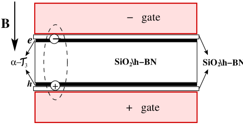
Figure 1: Schmematic illustration of a dipolar magnetoexciton on a pair of $\alpha$-${\cal T}_{3}$ layers embedded in an insulating material. A uniform perpendicular magnetic field ${\bf B}$ is applied, and negative and positive biases are attached to the layers in the $xy$-plane.

A schematic illustration of a dipolar magnetoexciton, which is a bound state of a spatially separated electron and a hole, located on a pair of $\alpha$-${\cal T}_{3}$ layers embedded in an insulating material in a perpendicular magnetic field ${\bf B}$, is depicted in Fig. 1. In the case of non-interacting excitons, the eigenvalues are additive and we obtain

$$\varepsilon_{n_{+},n_{-}}=\frac{\hbar v_{F}}{r_{B}}\sqrt{2}\Bigg{(}\text{sgn}(n_{+})\sqrt{n_{+}-\frac{1}{2}\left(1+\eta\cos 2\phi\right)}$$

$$\times\text{sgn}(n_{-})\sqrt{n_{+}-\frac{1}{2}\left(1-\eta\cos 2\phi\right)}\Bigg{)}\ .$$ (12)

The general eigenstates are a superposition of product states of the form

$$|\Psi_{n_{+},n_{-}}\rangle=|\psi_{n_{+}}\rangle\otimes|\psi_{n_{-}}\rangle$$

$$|\Psi\rangle=\sum_{n_{+},n_{-}}a(n_{+},n_{-})|\Psi_{n_{+},n_{-}}\rangle\ .$$

We now rewrite the Hamiltonian in the center-of-mass (CM) and relative coordinates. The energy of indirect excitons is obtained when a substrate is sandwiched between a double-layer of $\alpha$-${\cal T}_{3}$. We then have the Coulomb term $u({\bf r}_{e}-{\bf r}_{h})$ between electron at ${\bf r}_{e}$ and hole at ${\bf r}_{h}$. The magneto-exciton Hamiltonian is given by

$$H =H^{e}_{kin}\otimes\mathds{1}_{h}+\mathds{1}_{e}\otimes H^{h}_{kin}+u({\bf r}_{e}-{\bf r}_{h})\otimes\mathds{1}$$ (13)

$$=\hbar v_{F}\begin{pmatrix}0&\cos\phi[p_{ex}+i(p_{ey}+eBx_{e})]&0\\ \cos\phi[p_{ex}-i(p_{ey}+eBx_{e})]&0&\sin\phi[p_{ex}+i(p_{ey}+eBx_{e})]\\ 0&\sin\phi[p_{ex}-i(p_{ey}+eBx_{e})]&0\\ \end{pmatrix}\otimes\mathds{1}_{h}$$

$$+\hbar v_{F}\mathds{1}_{e}\otimes\begin{pmatrix}0&\cos\phi[p_{hx}-i(p_{hy}-eBx_{h})]&0\\ \cos\phi[p_{hx}+i(p_{hy}-eBx_{h})]&0&\sin\phi[p_{hx}-i(p_{hy}-eBx_{h})]\\ 0&\sin\phi[p_{hx}+i(p_{hy}-eBx_{h})]&0\\ \end{pmatrix}$$

We go to center of mass and relative coordinate system as follows.

$${\bf p}_{e/h}={\bf P}/2\pm{\bf p},\;\;\;\;{\bf r}_{e/h}={\bf R}\pm{\bf r}/2$$

We define the pseudospin-1 operators $S_{x}(\phi)$ and $S_{y}(\phi)$ as

$$S_{x}(\phi)=\begin{pmatrix}0&\cos\phi&0\\ \cos\phi&0&\sin\phi\\ 0&\sin\phi&0\\ \end{pmatrix}\;\;\;\;\;\;S_{y}(\phi)=i\begin{pmatrix}0&-\cos\phi&0\\ \cos\phi&0&-\sin\phi\\ 0&\sin\phi&0\\ \end{pmatrix}$$

The total Hamiltonian is then given by

$$H= \hbar v_{F}\Big{(}P_{x}m^{+}_{x}(\phi)+2p_{x}m^{-}_{x}(\phi)+(P_{y}-eBx)m^{-}_{y}(\phi)+2p_{y}m^{+}_{y}(\phi)$$

$$+2(p_{y}+eBX)m^{+}_{y}(\phi)\Big{)}+u({\bf r})\otimes\mathds{1}$$

In this notation,

$$m^{\pm}_{x}(\phi)=\frac{1}{2}\left[S_{x}(\phi)\otimes\mathds{1}_{h}\pm\mathds{1}_{e}\otimes S_{x}(\phi)\right]$$

$$m^{\pm}_{y}(\phi)=\frac{1}{2}\left[S_{y}(\phi)\otimes\mathds{1}_{h}\pm\mathds{1}_{e}\otimes S_{y}(\phi)\right]\ .$$

The unitary operator $U=e^{ieBXy}$ transforms the Hamiltonian

$$U^{\dagger}HU=\hbar v_{F}\Big{(}2{\bf p}\cdot{\bf m}^{-}(\phi)+(\bf{P}-\hat{z}\times{\bf r})\cdot{\bf m}^{+}(\phi)\Big{)}+u({\bf r})\otimes\mathds{1}$$

shifting ${\bf r}\to{\bf r-\hat{z}}\times{\bf P}$, moves the ${\bf P}$ dependence to the potential energy. This gives the same form of two-particle wave function as in BLG . Here are the states and the energies in the notation and form as BLG (see Eqs. 4 and 6). The nine-component wave function is written as follows. Note the symbols have the same definitions as BLG . We have

$$\Psi({\bf R},{\bf r})=\exp\left[i\left({\bf P}+\frac{e}{2c}[{\bf B}\times{\bf r}]\right)\cdot\frac{{\bf R}}{\hbar}\right]\tilde{\Phi}({\bf r}-{\bf{\bm{\rho}}}_{0})\ .$$ (14)

III.1 Magnetoexciton states for $n_{+},\,n_{-}=2,\,3,\cdots$

We assume that both electrons and holes are in the $K$ valley and we first consider $n_{+}=2,\,3,\cdots$ and $n_{-}=2,\,3,\cdots$ states. Therefore, for a magnetoexciton state, we use the tensor product of the above states for the electron-hole wave function. We express the wave function using

$$\Phi_{n_{+},n_{-}}({\bf r})=(2\pi)^{-1/2}2^{-|m|/2}\frac{\tilde{n}!}{\sqrt{n_{+}!n_{-}!}}\frac{1}{r_{B}}\text{sgn}(m)^{m}\frac{r^{|m|}}{r^{|m|}_{B}}\exp\left[-im\phi-\frac{r^{2}}{4r^{2}_{B}}\right]L^{|m|}_{\tilde{n}}\left(\frac{r^{2}}{2r^{2}_{B}}\right)\ ,$$ (15)

where $m=\left|n_{+}-n_{-}\right|$, $\tilde{n}=\min(n_{+},n_{-})$ and $L$ are Laguerre polynomials. We have

$$\psi_{n_{+}}({\bf r}_{e})\otimes\psi_{n_{-}}({\bf r}_{h})=\frac{1}{2}\begin{pmatrix}a_{n_{+}}(\phi)\Phi_{n_{+}-2}({\bf r}_{e})\\ \Phi_{n_{+}-1}({\bf r}_{e})\\ b_{n_{+}}(\phi)\Phi_{n_{+}}({\bf r}_{e})\\ \end{pmatrix}\otimes\begin{pmatrix}a_{n_{-}}(\phi)\Phi_{n_{-}-2}({\bf r}_{h})\\ -\Phi_{n_{-}-1}({\bf r}_{h})\\ b_{n_{-}}(\phi)\Phi_{n_{-}}({\bf r}_{h})\\ \end{pmatrix}\ .$$ (16)

This leads to the following wave function in the CM coordinate frame of reference.

$$\tilde{\Phi}_{n_{+},n_{-}}({\bf r})=\frac{1}{2}\begin{pmatrix}a_{n_{+}}(\phi)a_{n_{-}}(\phi)\Phi_{n_{+}-2,n_{-}-2}({\bf r})\\ -a_{n_{+}}(\phi)\Phi_{n_{+}-2,n_{-}-1}({\bf r})\\ a_{n_{+}}(\phi)b_{n_{-}}(\phi)\Phi_{n_{+}-2,n_{-}}({\bf r})\\ a_{n_{-}}(\phi)\Phi_{n_{+}-1,n_{-}-2}({\bf r})\\ -\Phi_{n_{+}-1,n_{-}-1}({\bf r})\\ b_{n_{-}}(\phi)\Phi_{n_{+}-1,n_{-}}({\bf r})\\ b_{n_{+}}(\phi)a_{n_{-}}(\phi)\Phi_{n_{+},n_{-}-2}({\bf r})\\ -b_{n_{+}}(\phi)\Phi_{n_{+},n_{-}-1}({\bf r})\\ b_{n_{+}}(\phi)a_{n_{-}}(\phi)\Phi_{n_{+},n_{-}}({\bf r})\\ \end{pmatrix}\ .$$ (17)

III.2 Landau-Levels for $n_{\pm}=1$

The $n_{\pm}=1$ Landau-Levels are treated separately as described below. We express the eigenvalue problem as

$$H^{e}_{kin}|\Psi\rangle=\gamma_{B}\begin{pmatrix}0&c_{+}\cos\phi&0\\ c^{\dagger}_{+}\cos\phi&0&c_{+}\sin\phi\\ 0&c^{\dagger}_{+}\sin\phi&0\\ \end{pmatrix}\begin{pmatrix}0\\ \alpha|0\rangle\\ \beta|1\rangle\\ \end{pmatrix}=\varepsilon\begin{pmatrix}0\\ \alpha|0\rangle\\ \beta|1\rangle\\ \end{pmatrix}$$ (18)

and we have a similar equation for a hole from which the states are given by

$$\psi_{n_{+}=1}({\bf r}_{e})=\frac{1}{\sqrt{2}}\begin{pmatrix}0\\ \pm\Phi_{0}({\bf r}_{e})\\ \Phi_{1}({\bf r}_{e})\\ \end{pmatrix},\;\;\;\;\;\psi_{n_{-}=1}({\bf r}_{h})=\frac{1}{\sqrt{2}}\begin{pmatrix}0\\ \pm\Phi_{0}({\bf r}_{h})\\ \Phi_{1}({\bf r}_{h})\\ \end{pmatrix}$$ (19)

We note that the $n_{\pm}=1$ states are independent of the hopping parameter $\phi$

III.3 Magnetoexciton states for $n_{+}=2,\,3,\cdots\;\;\;n_{-}=1$

$$\psi_{n_{+}}({\bf r}_{e})\otimes\psi_{n_{-}}({\bf r}_{h})=\frac{1}{2}\begin{pmatrix}a_{n_{+}}(\phi)\Phi_{n_{+}-2}({\bf r}_{e})\\ \Phi_{n_{+}-1}({\bf r}_{e})\\ b_{n_{+}}(\phi)\Phi_{n_{+}}({\bf r}_{e})\\ \end{pmatrix}\otimes\begin{pmatrix}0\\ -\Phi_{0}({\bf r}_{h})\\ \Phi_{1}({\bf r}_{h})\\ \end{pmatrix}$$ (20)

This leads to the following wave function in the CM coordinate system.

$$\tilde{\Phi}_{n_{+},n_{-}}({\bf r})=\frac{1}{2}\begin{pmatrix}0\\ -a_{n_{+}}(\phi)\Phi_{n_{+}-2,0}({\bf r})\\ a_{n_{+}}(\phi)\Phi_{n_{+}-2,1}({\bf r})\\ 0\\ -\Phi_{n_{+}-1,0}({\bf r})\\ \Phi_{n_{+}-1,1}({\bf r})\\ 0\\ -b_{n_{+}}(\phi)\Phi_{n_{+},0}({\bf r})\\ b_{n_{+}}(\phi)\Phi_{n_{+},1}({\bf r})\\ \end{pmatrix}$$ (21)

III.4 Magnetoexciton states for $n_{+}=1,\;\;\;n_{-}=2,\,3,\cdots$

$$\psi_{n_{+}}({\bf r}_{e})\otimes\psi_{n_{-}}({\bf r}_{h})=\frac{1}{2}\begin{pmatrix}0\\ \Phi_{0}({\bf r}_{e})\\ \Phi_{1}({\bf r}_{e})\\ \end{pmatrix}\otimes\begin{pmatrix}a_{n_{-}}(\phi)\Phi_{n_{-}-2}({\bf r}_{h})\\ -\Phi_{n_{-}-1}({\bf r}_{h})\\ b_{n_{-}}(\phi)\Phi_{n_{-}}({\bf r}_{h})\\ \end{pmatrix}$$ (22)

This leads to the following wave function in the CM coordinate system.

$$\tilde{\Phi}_{1,n_{-}}({\bf r})=\frac{1}{2}\begin{pmatrix}0\\ 0\\ 0\\ a_{n_{-}}(\phi)\Phi_{0,n_{-}-2}({\bf r})\\ -\Phi_{0,n_{-}-1}({\bf r})\\ b_{n_{-}}(\phi)\Phi_{0,n_{-}}({\bf r})\\ a_{n_{-}}(\phi)\Phi_{1,n_{-}-2}({\bf r})\\ -\Phi_{1,n_{-}-1}({\bf r})\\ b_{n_{-}}(\phi)\Phi_{1,n_{-}}({\bf r})\\ \end{pmatrix}$$ (23)

III.5 Magnetoexciton states for $n_{+}=1\;\;n_{-}=1$

We note that for $n=0$ we have no valence or conduction band states, but there is a flat band described by

$$\psi_{n_{+}=1}({\bf r}_{e})\otimes\psi_{n_{-}=1}({\bf r}_{h})=\frac{1}{2}\begin{pmatrix}0\\ +\Phi_{0}({\bf r}_{e})\\ \Phi_{1}({\bf r}_{e})\\ \end{pmatrix}\otimes\begin{pmatrix}0\\ -\Phi_{0}({\bf r}_{h})\\ \Phi_{1}({\bf r}_{h})\\ \end{pmatrix}$$ (24)

which yields the following wave function in the CM frame of reference as

$$\tilde{\Phi}_{n_{+}=1,n_{-}=1}({\bf r})=\frac{1}{2}\begin{pmatrix}0\\ 0\\ 0\\ 0\\ -\Phi_{0,0}({\bf r})\\ \Phi_{0,1}({\bf r})\\ 0\\ \Phi_{1,0}({\bf r})\\ \Phi_{1,1}({\bf r})\\ \end{pmatrix}\ .$$ (25)

III.6 Magnetoexciton states for $n_{+}=1\;\;n_{-}=0$

For the case when $n=0$, there is neither a valence nor conduction band, but there is a flat-band. We now consider an electron in $n_{+}=1$ and a hole in the flat band with $n_{-}=0$. The $n=0$ state

$$\psi_{n_{-}=0}({\bf r}_{h})\ =\begin{pmatrix}0\\ 0\\ \Phi_{0}({\bf r}_{h})\\ \end{pmatrix}\ .$$ (26)

The corresponding exciton state becomes

$$\psi_{n_{+}=1}({\bf r}_{e})\otimes\psi_{n_{-}=0}({\bf r}_{h})=\frac{1}{\sqrt{2}}\begin{pmatrix}0\\ \Phi_{0}({\bf r}_{e})\\ \Phi_{1}({\bf r}_{e})\\ \end{pmatrix}\otimes\begin{pmatrix}0\\ 0\\ \Phi_{0}({\bf r}_{h})\\ \end{pmatrix}\ .$$ (27)

This leads to the following wave function in the CM coordinate system.

$$\tilde{\Phi}_{n_{+}=1,n_{-}=0}({\bf r})=\frac{1}{\sqrt{2}}\begin{pmatrix}0\\ 0\\ 0\\ 0\\ 0\\ \Phi_{0,0}({\bf r})\\ 0\\ 0\\ \Phi_{1,0}({\bf r})\\ \end{pmatrix}\ .$$ (28)

IV Isolated dipolar magnetoexciton

For case 1, we calculate the magnetoexciton energy using the expectation value for an electron in Landau level $1$ and a hole in level $1$. In high magnetic field, the magnetoexciton is constructed from an electron and hole in the lowest Landau level with the following nine-component wave function having relative coordinates

$$\tilde{\Phi}_{1,1}(\mathbf{r})=\left(\begin{array}[]{c}0\\ 0\\ 0\\ 0\\ -\Phi_{0,0}(\mathbf{r})\\ \Phi_{0,1}(\mathbf{r})\\ 0\\ \Phi_{1,0}(\mathbf{r})\\ \Phi_{1,1}(\mathbf{r})\end{array}\right)\ .$$ (38)

For case 2, we calculate the magnetoexciton energy using the expectation value for an electron in Landau level $1$ and a hole in level $0$. We have

$$\tilde{\Phi}_{1,0}(\mathbf{r})=\left(\begin{array}[]{c}0\\ 0\\ 0\\ 0\\ 0\\ \Phi_{0,0}(\mathbf{r})\\ 0\\ 0\\ \Phi_{1,0}(\mathbf{r})\end{array}\right)\ .$$ (48)

The 2D harmonic oscillator eigenfunctions $\Phi_{n_{e},n_{h}}(\mathbf{r})$ are given by Iyengar

$$\Phi_{n_{e},n_{h}}(\mathbf{r})=(2\pi)^{-1/2}2^{-|m|/2}\frac{\tilde{n}!}{\sqrt{n_{1}!n_{2}!}}\frac{1}{r_{B}}\mathrm{sgn}(m)^{m}\frac{r^{|m|}}{r_{B}^{|m|}}\exp\left[-im\phi-\frac{r^{2}}{4r_{B}^{2}}\right]L_{\tilde{n}}^{|m|}\left(\frac{r^{2}}{2r_{B}^{2}}\right)\ ,$$ (49)

where $r_{B}=\sqrt{\hbar/(eB)}$ is the magnetic length, $L_{\tilde{n}}^{|m|}(x)$ denotes Laguerre polynomials; $m=n_{e}-n_{h}$; $\tilde{n}=\min(n_{e},n_{h})$, and $\mathrm{sgn}(m)^{m}=1$ for $m=0$.

The magnetoexciton energy in high magnetic field can be calculated by employing perturbation theory with respect to Coulombic electron-hole attraction analogously to 2D quantum wells with finite electron and hole masses Lerner . This approach allows us to derive the spectrum of isolated dipolar magnetoexcitons with spatially separated electrons and holes in the $\alpha$-${\cal T}_{3}$ double layer. For the $\alpha$-${\cal T}_{3}$ double layer, this perturbation theory is valid only for relatively large separation $D$ between electron and hole $\alpha$-${\cal T}_{3}$ double layers and relatively high magnetic fields $B$, i.e., $D\gg r_{B}$ when $e^{2}/(\epsilon D)\ll\hbar v_{F}/r_{B}$. Here, $e^{2}/(\epsilon D)$ is the characteristic Coulomb electron-hole attraction for the $\alpha$-${\cal T}_{3}$ double layer and $\hbar v_{F}/r_{B}$ is the energy difference between the first and zeroth Landau levels in $\alpha$-${\cal T}_{3}$. The operator of electron-hole Coulomb attraction is

$$\hat{V}(r)=-\frac{ke^{2}}{\epsilon\sqrt{r^{2}+D^{2}}}\ ,$$ (50)

where $k=9\times 10^{9}\ N\times m^{2}/C^{2}$, $\epsilon$ is the dielectric constant of the insulator (SiO₂ or $h$-BN), surrounding the electron and hole $\alpha$-${\cal T}_{3}$ monolayers, forming the double layer; $D$ is the separation between electron and hole $\alpha$-${\cal T}_{3}$ mono-layers. For the $h$-BN barrier we substitute the dielectric constant $\epsilon=4.89$, while for the SiO₂ barrier we substitute the dielectric constant $\epsilon=4.5$.

The magnetoexciton energies $E_{n_{+},n_{-}}(P)$ in first order perturbation theory are given by

$$E_{n_{e},n_{h}}(P)=E_{n_{e},n_{h}}^{(0)}+\mathcal{E}_{n_{e},n_{h}}(P)\ ,$$ (51)

where $E_{n_{e},n_{h}}^{(0)}$ is the unperturbed spectrum, and

$$\mathcal{E}_{n_{e},n_{h}}(P)=-\left\langle n_{e}n_{h}\mathbf{P}\left|\frac{ke^{2}}{\epsilon\sqrt{D^{2}+r^{2}}}\right|n_{e}n_{h}\mathbf{P}\right\rangle\ .$$ (52)

Neglecting the transitions between different Landau levels, first order perturbation woth respect to the Coulomb attraction leads to the following result for the energy of magnetoexciton for case 1:

$$\mathcal{E}_{1,1}(P)=-\left\langle 1,1,\mathbf{P}\left|\frac{ke^{2}}{\epsilon\sqrt{D^{2}+r^{2}}}\right|1,1,\mathbf{P}\right\rangle,$$ (53)

and for case 2:

$$\mathcal{E}_{1,0}(P)=-\left\langle 1,0,\mathbf{P}\left|\frac{ke^{2}}{\epsilon\sqrt{D^{2}+r^{2}}}\right|1,0,\mathbf{P}\right\rangle\ .$$ (54)

Denoting the averaging involving the 2D harmonic oscillator eigenfunctions $\Phi_{n_{e},n_{h}}(\mathbf{r})$ in Eq. (49) as $\langle\langle\tilde{n}m\mathbf{P}|\cdots|\tilde{n}m\mathbf{P}\rangle\rangle$ ($\tilde{n}$ and $m$ are defined below Eq. (49)), we obtain the energy of an indirect magnetoexciton created by spatially separated electrons and holes in the lowest Landau level for case 1:

$$\mathcal{E}_{1,1}(P) = \left\langle 1,1,\mathbf{P}\left|\hat{V}(r)\right|1,1,\mathbf{P}\right\rangle=\frac{1}{4}\left[\left\langle\left\langle 0,0,\mathbf{P}\left|\hat{V}(r)\right|0,0,\mathbf{P}\right\rangle\right\rangle\right.$$ (55)

$$+ \left.2\left\langle\left\langle 0,1,\mathbf{P}\left|\hat{V}(r)\right|0,1,\mathbf{P}\right\rangle\right\rangle+\left\langle\left\langle 1,0,\mathbf{P}\left|\hat{V}(r)\right|1,0,\mathbf{P}\right\rangle\right\rangle\right]$$

and for case 2, we have

$$\mathcal{E}_{1,0}(P) = \left\langle 1,0,\mathbf{P}\left|\hat{V}(r)\right|1,0\mathbf{P}\right\rangle=\frac{1}{2}\left[\left\langle\left\langle 0,0,\mathbf{P}\left|\hat{V}(r)\right|0,0,\mathbf{P}\right\rangle\right\rangle\right.$$ (56)

$$+ \left.\left\langle\left\langle 0,1,\mathbf{P}\left|\hat{V}(r)\right|0,1,\mathbf{P}\right\rangle\right\rangle\right]\ .$$

Substituting for small magnetic momenta $P\ll\hbar/r_{B}$ and $P\ll\hbar D/r_{B}^{2}$ the following relations Ruvinsky

$$\langle\langle\tilde{n}m\mathbf{P}|\hat{V}(r)|\tilde{n}m\mathbf{P}\rangle\rangle=\mathcal{E}_{\tilde{n}m}^{(b)}+\frac{P^{2}}{2M_{\tilde{n}m}(B,D)}\ .$$ (57)

Making use of this in Eqs. (55) and (56), we obtain the dispersion law ofa magnetoexciton for small magnetic momenta in cases 1 and 2, correspondingly, i.e.,

$$\mathcal{E}_{1,1}(P) = \frac{1}{4}\left(\mathcal{E}_{00}^{(b)}(B,D)+2\mathcal{E}_{01}^{(b)}(B,D)+\mathcal{E}_{10}^{(b)}(B,D)\right)$$ (58)

$$+ \frac{1}{4}\left(\frac{1}{M_{00}(B,D)}+\frac{2}{M_{01}(B,D)}+\frac{1}{M_{10}(B,D)}\right)\frac{P^{2}}{2}$$

$$= -\mathcal{E}_{B}^{(b)}(D)+\frac{P^{2}}{2m_{B}(D)}\ ,$$

and

$$\mathcal{E}_{1,0}(P) = \frac{1}{2}\left(\mathcal{E}_{00}^{(b)}(B,D)+\mathcal{E}_{01}^{(b)}(B,D)\right)$$ (59)

$$+ \frac{1}{2}\left(\frac{P^{2}}{2M_{00}(B,D)}+\frac{P^{2}}{2M_{01}(B,D)}\right)=-\mathcal{E}_{B}^{(b)}(D)+\frac{P^{2}}{2m_{B}(D)}\ ,$$

where the binding energy $\mathcal{E}_{B}^{(b)}(D)$ and the effective magnetic mass $m_{B}(D)$ of a magnetoexciton with spatially separated electron and hole in the $\alpha$-${\cal T}_{3}$ double layer are for case 1

$$\mathcal{E}_{B}^{(b)}(D) = -\frac{1}{4}\left(\mathcal{E}_{00}^{(b)}(B,D)+2\mathcal{E}_{01}^{(b)}(B,D)+\mathcal{E}_{10}^{(b)}(B,D)\right),$$

$$\frac{1}{m_{B}(D)} = \frac{1}{4}\left(\frac{1}{M_{00}(B,D)}+\frac{2}{M_{01}(B,D)}+\frac{1}{M_{10}(B,D)}\right),$$ (60)

and for case 2:

$$\mathcal{E}_{B}^{(b)}(D) = -\frac{1}{2}\left(\mathcal{E}_{00}^{(b)}(B,D)+\mathcal{E}_{01}^{(b)}(B,D)\right),$$

$$\frac{1}{m_{B}(D)} = \frac{1}{2}\left(\frac{1}{M_{00}(B,D)}+\frac{1}{M_{01}(B,D)}\right),$$ (61)

where the constants $\mathcal{E}_{00}^{(b)}(B,D)$, $\mathcal{E}_{01}^{(b)}(B,D)$, $\mathcal{E}_{10}^{(b)}(B,D)$, $M_{00}(B,D)$, $M_{01}(B,D)$ and $M_{10}(B,D)$ depending on magnetic field $B$ and the inter-layer separation $D$ are defined by Ruvinsky

$$\mathcal{E}_{00}^{(b)}(B,D) = -\mathcal{E}_{0}\exp\left[\frac{D^{2}}{2r_{B}^{2}}\right]\mathrm{erfc}\left[\frac{D}{\sqrt{2}r_{B}}\right],$$

$$\mathcal{E}_{01}^{(b)}(B,D) = -\mathcal{E}_{0}\left[\left(\frac{1}{2}-\frac{D^{2}}{2r_{B}^{2}}\right)\exp\left[\frac{D^{2}}{2r_{B}^{2}}\right]\mathrm{erfc}\left[\frac{D}{\sqrt{2}r_{B}}\right]+\frac{D}{\sqrt{2\pi}r_{B}}\right],$$

$$\mathcal{E}_{10}^{(b)}(B,D) = -\mathcal{E}_{0}\left[\left(\frac{3}{4}+\frac{D^{2}}{2r_{B}^{2}}+\frac{D^{4}}{4r_{B}^{4}}\right)\exp\left[\frac{D^{2}}{2r_{B}^{2}}\right]\mathrm{erfc}\left[\frac{D}{\sqrt{2}r_{B}}\right]-\frac{D}{2\sqrt{2\pi}r_{B}}-\left(\frac{D}{\sqrt{2}r_{B}}\right)^{3}\frac{1}{\sqrt{\pi}}\right],$$

$$M_{00}(B,D) = M_{0}\left[\left(1+\frac{D^{2}}{r_{B}^{2}}\right)\exp\left[\frac{D^{2}}{2r_{B}^{2}}\right]\mathrm{erfc}\left[\frac{D}{\sqrt{2}r_{B}}\right]-\sqrt{\frac{2}{\pi}}\frac{D}{r_{B}}\right]^{-1},$$

$$M_{01}(B,D) = M_{0}\left[\left(3+\frac{D^{2}}{r_{B}^{2}}\right)\frac{D}{\sqrt{2\pi}r_{B}}-\left(\frac{1}{2}+2\frac{D^{2}}{r_{B}^{2}}+\frac{D^{4}}{2r_{B}^{4}}\right)\exp\left[\frac{D^{2}}{2r_{B}^{2}}\right]\mathrm{erfc}\left[\frac{D}{\sqrt{2}r_{B}}\right]\right]^{-1},$$

$$M_{10}(B,D) = M_{0}\left[\frac{1}{4}\left(7+25\frac{D^{2}}{r_{B}^{2}}+11\frac{D^{4}}{r_{B}^{4}}+\frac{D^{6}}{r_{B}^{6}}\right)\exp\left[\frac{D^{2}}{2r_{B}^{2}}\right]\mathrm{erfc}\left[\frac{D}{\sqrt{2}r_{B}}\right]\right.$$ (62)

$$- \left.\left(\frac{17}{2}+5\frac{D^{2}}{r_{B}^{2}}+\frac{D^{4}}{2r_{B}^{4}}\right)\frac{D}{\sqrt{2\pi}r_{B}}\right]^{-1}\ ,$$

where the constants $\mathcal{E}_{0}$ and $M_{0}$ and function $\mathrm{erfc}(z)$ are given by Ruvinsky

$$\mathcal{E}_{0} = \left\langle\left\langle 00\mathbf{P}\left|\frac{e^{2}}{\epsilon|\mathbf{r}|}\right|00\mathbf{P}\right\rangle\right\rangle_{\mathbf{P}=0}=\frac{ke^{2}}{\epsilon r_{B}}\sqrt{\frac{\pi}{2}},$$

$$M_{0} = -\left[2\left(\left\langle\left\langle 00\mathbf{P}\left|\frac{e^{2}}{\epsilon|\mathbf{r}|}\right|00\mathbf{P}\right\rangle\right\rangle-\mathcal{E}_{0}\right)\right]^{-1}P^{2}=\frac{2^{3/2}\epsilon\hbar^{2}}{\sqrt{\pi}ke^{2}r_{B}},$$

$$\mathrm{erfc}(z) = \frac{2}{\sqrt{\pi}}\int_{z}^{\infty}\exp\left(-t^{2}\right)dt\ .$$ (63)

For both cases 1 and 2, for large inter-layer separation $D\gg r_{B}$, the asymptotic values for the binding energy $\mathcal{E}_{B}^{(b)}(D)$ and the effective magnetic mass $m_{B}(D)$ of the dipolar magnetoexciton in the $\alpha$-${\cal T}_{3}$ double layer are the same and given by

$$\mathcal{E}_{B}^{(b)}(B,D)=\frac{ke^{2}}{\epsilon D},\ \ \ m_{B}(D)=\frac{\epsilon D^{3}B^{2}}{k}\ .$$ (64)

Measuring energy from the binding energy of the magnetoexciton, the dispersion relation $\varepsilon_{k}(P)$ for an isolated dipolar magnetoexciton is a quadratic function at small magnetic momentum $P\ll\hbar/r_{B}$ and $P\ll\hbar D/r_{B}^{2}$:

$$\varepsilon_{k}({\bf P})=\frac{P^{2}}{2m_{Bk}}\ ,$$ (65)

where $m_{Bk}$, the effective magnetic mass, dependent on $B$ and the separation $D$ between electron and hole layers as well as the quantum number $k$ ($k=(n_{e},n_{h})$ are magnetoexcitonic quantum numbers).

The squared 2D radius of a magnetoexciton for case 1 can be defined as

$$r_{1,1}^{2}(P=0) = \left\langle 1,1,\mathbf{P}\left|r^{2}\right|1,1,\mathbf{P}\right\rangle_{\mathbf{P}=0}=\frac{1}{4}\left(l_{00}^{2}+2l_{01}^{2}+l_{10}^{2}\right)=4r_{B}^{2},\hskip 28.45274ptr_{1,1}=2r_{B},$$ (66)

and for case 2 as

$$r_{1,0}^{2}(P=0) = \left\langle 1,0,\mathbf{P}\left|r^{2}\right|1,0,\mathbf{P}\right\rangle_{\mathbf{P}=0}=\frac{1}{2}\left(l_{00}^{2}+l_{01}^{2}\right)=3r_{B}^{2},\hskip 28.45274ptr_{1,0}=\sqrt{3}r_{B}\ ,$$ (67)

where $l_{\tilde{n}m}^{2}=\left\langle\left\langle\tilde{n}m\mathbf{P}\left|\hat{r^{2}}\right|\tilde{n}m\mathbf{P}\right\rangle\right\rangle_{\mathbf{P}=0}$ and ($l_{00}^{2}=2r_{B}^{2}$, $l_{01}^{2}=4r_{B}^{2}$, $l_{10}^{2}=6r_{B}^{2}$) Ruvinsky .

V Superfluidity of dipolar magnetoexcitons in an $\alpha$-${\cal T}_{3}$ double layer

Dipolar magnetoexcitons have electrical dipole moments, produced by the inter-layer separation $D$. We assume, that dipolar magnetoexcitons repel each other like parallel dipoles. The latter assumption is reasonable when $D$ is larger than the mean separation between an electron and hole parallel to the $\alpha$-${\cal T}_{3}$ layers $D\gg\left(\langle r^{2}\rangle\right)^{1/2}$.

Since electrons on an $\alpha$-${\cal T}_{3}$ monolayer can be located in two valleys, there are four types of dipolar magnetoexcitons in an $\alpha$-${\cal T}_{3}$ double layer. Since all these types of dipolar magnetoexcitons have identical envelope wave functions and energies, it is reasonable to assume that a dipolar magnetoexciton is located in only one valley. We use $n_{0}=n/(4s)$ as the density of magnetoexcitons in one valley, where $n$ is the total density of magnetoexcitons, $s$ is the spin degeneracy ( $s=4$ for magnetoexcitons in an $\alpha$-${\cal T}_{3}$ double layer).

We shall treat a dilute 2D magnetoexciton system in the $\alpha$-${\cal T}_{3}$ double layer as a weakly interacting Bose gas by applying the procedure, described in Ref. BLG . Two dipolar magnetoexcitons in a dilute system repel each other with the potential energy of the pair magnetoexciton-magnetoexciton interaction, written as $U(R)=ke^{2}D^{2}/(\epsilon R^{3})$, where $R$ is the distance between magnetoexciton dipoles along the $\alpha$-${\cal T}_{3}$ layers. For the weakly interacting Bose gas of 2D dipolar magnetoexcitons (when $na^{2}(B)\ll 1$, where $a(B)$ is the in-plane radius of a dipolar magnetoexciton defined for cases 1 and 2 in Eqs. (66) and (67), respectively) the summation of ladder diagrams is valid Abrikosov . The chemical potential $\mu$, corresponding to the summation of the ladder diagrams, can be written as BLG

$$\mu=\frac{\kappa^{2}}{2m_{B}}=\frac{\pi\hbar^{2}n}{sm_{B}\log\left[s\hbar^{4}\epsilon^{2}/\left(2\pi nm_{B}^{2}k^{2}e^{4}D^{4}\right)\right]}\ ,$$ (68)

where $s=4$ is the spin degeneracy factor.

The spectrum of collective excitations, obtained from the ladder approximation, at low magnetic momenta corresponds to the sound spectrum of collective excitations $\varepsilon(P)=c_{s}P$ with the sound velocity $c_{s}=\sqrt{\mu/m_{B}}$, where $\mu$ is defined by Eq. (68). Since magnetoexcitons have a sound spectrum for collective excitations at small magnetic momenta $P$ due to dipole-dipole repulsion, the magnetoexcitonic superfluidity is possible at low temperatures $T$ in $\alpha$-${\cal T}_{3}$ double layers because the sound spectrum satisfies the Landau criterion for superfluidity Abrikosov ; Griffin .

The magnetoexcitons constructed from spatially separated electrons and holes in the $\alpha$-${\cal T}_{3}$ double layers with large inter-layer separation $D\gg r_{B}$ form a weakly interacting 2D gas of bosons with a dipole-dipole pair repulsion. Consequently, the superfluid-normal phase transition in this system is the Kosterlitz-Thouless transition Kosterlitz . The temperature $T_{c}$ of this phase change to the superfluid state in a 2D magnetoexciton system is determined by the equation

$$T_{c}=\frac{\pi\hbar^{2}n_{s}(T_{c})}{2k_{B}m_{B}}\ ,$$ (69)

where $n_{s}(T)$ is the superfluid density of the magnetoexciton system as a function of temperature $T$, magnetic field $B$, inter-layer separation $D$; and $k_{B}$ is the Boltzmann constant. The function $n_{s}(T)$ in Eq.  (69) can be determined from the relation $n_{s}=n/(4s)-n_{n}$, where $n$ is the total density, $n_{n}$ is the normal component density. Following the procedure, described in Ref. [BLG, ], we have for the superfluid density

$$n_{s}=\frac{n}{4s}-n_{n}=\frac{n}{4s}-\frac{3\zeta(3)}{2\pi\hbar^{2}}\frac{k_{B}^{3}T^{3}}{c_{s}^{4}m_{B}}\ .$$ (70)

In a 2D system, superfluidity of magnetoexcitons appears below the Kosterlitz-Thouless transition temperature (Eq. (69)), where only coupled vortices are present Kosterlitz . Using Eq. (70) for the density $n_{s}$ of the superfluid component, we obtain an equation for the Kosterlitz-Thouless transition temperature $T_{c}$. Its solution is

$$T_{c}=\left[\left(1+\sqrt{\frac{32}{27}\left(\frac{sm_{B}k_{B}T_{c}^{0}}{\pi\hbar^{2}n}\right)^{3}+1}\right)^{1/3}-\left(\sqrt{\frac{32}{27}\left(\frac{sm_{B}k_{B}T_{c}^{0}}{\pi\hbar^{2}n}\right)^{3}+1}-1\right)^{1/3}\right]\frac{T_{c}^{0}}{2^{1/3}}\ .$$ (71)

Here, $T_{c}^{0}$ is the temperature at which the superfluid density vanishes in the mean-field approximation (i.e., $n_{s}(T_{c}^{0})=0$),

$$T_{c}^{0}=\frac{1}{k_{B}}\left(\frac{\pi\hbar^{2}nc_{s}^{4}m_{B}}{6s\zeta(3)}\right)^{1/3}\ .$$ (72)

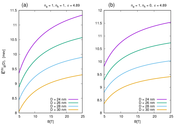
Figure 2: (Color online)   The magnetoexciton binding energy $\mathcal{E}_{B}^{b}(B,D)$ as a function of magnetic field $B$ for chosen interlayer separations $D$ for (a) case 1 on the left-hand side and (b) case 2, on the right.

In Fig.  2, we present results showing the dependence of the magnetoexciton binding energy $\mathcal{E}_{B}^{b}(B,D)$ on the magnetic field $B$ for chosen interlayer separation $D$ in case 1 and case 2, respectively. According to Fig. 2, $\mathcal{E}_{B}^{b}(B,D)$ is increased as $B$ is increased and $D$ is decreased. For the same parameters $\mathcal{E}_{B}^{b}(B,D$ is slightly larger for case 2 than case 1.

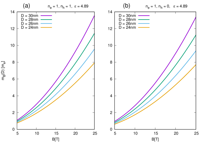
Figure 3: (Color online)  The effective magnetic mass $m_{B}(B,D)$ of a magnetoexciton as a function of magnetic field $B$ for chosen interlayer separation $D$ for (a) case 1 on the left-hand side and (b) case 2, on the right.

Figure 3 presents our results for the dependence of the effective magnetic mass $m_{B}(B,D)$ of a magnetoexciton on the magnetic field $B$ for chosen interlayer separation $D$ for cases 1 and 2. According to Fig. 3, $m_{B}(B,D)$ is increased as $B$ is increased and $D$ is increased. For the same parameters, $m_{B}(B,D)$ is slightly larger for case 1 compared with case 2.

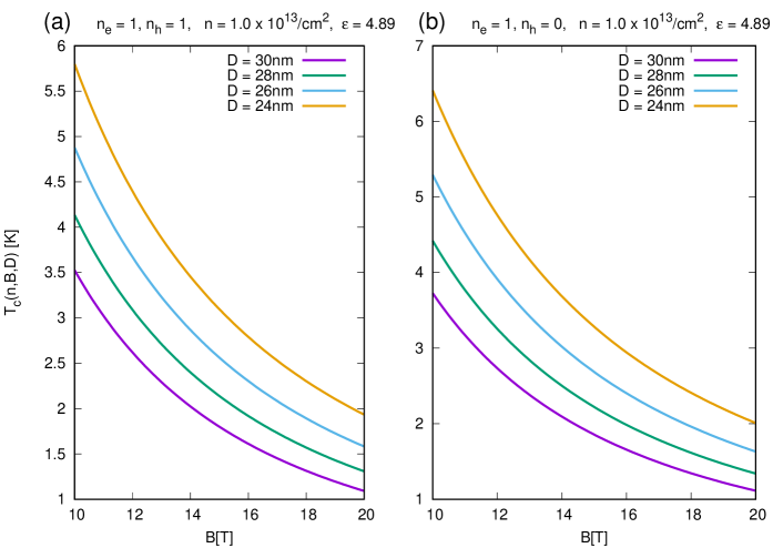
Figure 4: (Color online) The Kosterlitz-Thouless transition temperature $T_{c}(n,B,D)$ versus magnetic field $B$ for chosen interlayer separations $D$ at the fixed magnetoexciton concentration $n$ for (a) case 1 on the left-hand side and (b) case 2, on the right.

In Fig. 4, we display our results for the Kosterlitz-Thouless transition temperature $T_{c}(n,B,D)$ versus the magnetic field $B$ for various interlayer separations at fixed magnetoexciton concentration $n$ for cases 1 and 2. According to Fig. 4, $T_{c}(n,B,D)$ is decreased as $B$ is increased and $D$ is increased. For the same parameters, $T_{c}(n,B,D)$ is slightly larger for case 2 compared with case 1.

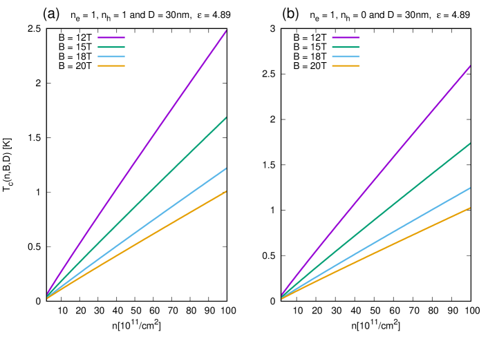
Figure 5: (Color online)  The Kosterlitz-Thouless transition temperature $T_{c}(n,B,D)$ as a function of the magnetoexciton concentration $n$ for various magnetic fields $B$ and fixed interlayer separation $D$ for (a) case 1 on the left-hand side and (b) case 2, on the right.

We have plotted in Fig.  5 the functional dependence of the Kosterlitz-Thouless transition temperature $T_{c}(n,B,D)$ on the magnetoexciton concentration $n$ for several chosen magnetic fields $B$ and fixed interlayer separation $D$ in both case 1 and 2. We deduce from Fig. 5 that $T_{c}(n,B,D)$ is increased as $n$is increased but is decreases ad as $B$ is increased. Additionally, we conclude that for the same values of the parameters, $T_{c}(n,B,D)$ is slightly larger for case 2 than case 1.

Based on Figs. 2, 4 and 5, one can conclude that case 2 is slightly more preferable than case 1 for observing dipolar magnetoexcitons and their superfluidity in the $\alpha$-${\cal T}_{3}$ double layer, since case 2 corresponds to slightly larger magnetoexciton binding energy $\mathcal{E}_{B}^{b}(B,D)$ as well as the Kosterlitz-Thouless transition temperature $T_{c}(n,B,D)$ than case 1 for the same described parameters.

VI Conclusions

In this paper, we have proposed the occurrence of BEC and superfluidity of dipolar magnetoexcitons in $\alpha$-${\cal T}_{3}$ double layers in a strong uniform perpendicular magnetic field. The low-energy Hamiltonian for a single $\alpha$-${\cal T}_{3}$ layer was obtained by including additional hopping terms to a single layer graphene Dirac Hamiltonian. We have found the solution of a two-body problem for an electron and a hole for the model Hamiltonian for the $\alpha$-${\cal T}_{3}$ double layer in a magnetic field. We have calculated the binding energy, effective mass, spectrum of collective excitations, superfluid density and the temperature of the Kosterlitz-Thouless phase transition to the superfluid state for dipolar magnetoexcitons in the $\alpha$-${\cal T}_{3}$ double layer. We have demonstrated that at fixed exciton density, the Kosterlitz-Thouless temperature for superfluidity of dipolar magnetoexcitons is decreased as a function of magnetic field. Our results show that $T_{c}$ is increased as a function of the density $n$ and is decreased as a function of the magnetic field $B$ and the interlayer separation $D$. We have demonstrated that case 2 (the dipolar magnetoexciton is formed by an electron in Landau level $1$ and hole in Landau level $0$) is slightly more preferable than case 1 (the dipolar magnetoexciton is formed by an electron in Landau level $1$ and hole in Landau level $-1$) to observe the dipolar magnetoexcitons and their superfluidity in $\alpha$-${\cal T}_{3}$ double layers. The reason is that case 2 corresponds to slightly larger magnetoexciton binding energy and Kosterlitz-Thouless transition temperature than case 1 for the same chosen parameters.

References

• (1) Yu. E. Lozovik and V. I. Yudson, Sov. Phys. JETP Lett. 22, 26 (1975); Sov. Phys. JETP 44, 389 (1976).
• (2) D. W. Snoke, Science 298, 1368 (2002).
• (3) L. V. Butov, J. Phys.: Condens. Matter 16, R1577 (2004).
• (4) J. P. Eisenstein and A. H. MacDonald, Nature 432, 691 (2004).
• (5) D. W. Snoke, in Quantum Gases: Finite Temperature and Non-equilibrium Dynamics, edited by N. P. Proukakis, S. A. Gardiner, M. J. Davis, and M. H. Szymanska, Cold Atom Series Vol. 1 (Imperial College Press, London, 2013), p. 419.
• (6) A. Perali, D. Neilson, and A. R. Hamilton, Phys. Rev. Lett. . 110, 146803 (2013).
• (7) O. L. Berman, Yu. E. Lozovik, and G. Gumbs, Phys. Rev. B 77, 155433 (2008).
• (8) Yu. E. Lozovik and A. A. Sokolik, JETP Lett. 87, 55 (2008); Phys. Lett. A 374, 326 (2009).
• (9) R. Bistritzer and A. H. MacDonald, Phys. Rev. Lett. 101, 256406 (2008).
• (10) O. L. Berman, R. Ya. Kezerashvili, and K. Ziegler, Phys. Rev. B 85, 035418 (2012).
• (11) M. M. Fogler, L. V. Butov, and K. S. Novoselov, Nature Commun. 5, 4555 (2014).
• (12) F.-C. Wu, F. Xue, and A. H. MacDonald, Phys. Rev. B 92, 165121 (2015).
• (13) O. L. Berman and R. Ya. Kezerashvili, Phys. Rev. B93, 245410 (2016).
• (14) O. L. Berman and R. Ya. Kezerashvili, Phys. Rev. B96, 094502 (2017).
• (15) O. L. Berman, G. Gumbs, and R. Ya. Kezerashvili, Phys. Rev. B96, 014505 (2017).
• (16) S. Saberi-Pouya, M. Zarenia, A. Perali, T. Vazifehshenas, and F. M. Peeters, Phys. Rev. B97, 174503 (2018).
• (17) I. V. Lerner and Yu. E. Lozovik, JETP 51, 588 (1980); JETP 53, 763 (1981); A. B. Dzyubenko and Yu. E. Lozovik, J. Phys. A 24, 415 (1991).
• (18) D. Paquet, T. M. Rice, and K. Ueda, Phys. Rev. B32, 5208 (1985).
• (19) C. Kallin and B. I. Halperin, Phys. Rev. B30, 5655 (1984); Phys. Rev. B31, 3635 (1985).
• (20) D. Yoshioka and A. H. MacDonald, J. Phys. Soc. Jpn 59, 4211 (1990).
• (21) Yu. E. Lozovik and A. M. Ruvinsky, Phys. Lett. A 227, 271 (1997); JETP 85, 979 (1997).
• (22) M. A. Olivares-Robles and S. E. Ulloa, Phys. Rev. B64, 115302 (2001).
• (23) S. A. Moskalenko, M. A. Liberman, D. W. Snoke and V. V. Botan, Phys. Rev. B66, 245316 (2002).
• (24) A. Raoux, M. Morigi, J.-N. Fuchs, F. Piéchon, and G. Montambaux, Phys. Rev. Lett. 112, 026402 (2014).
• (25) B. Sutherland, Phys. Rev. B 34, 5208 (1986).
• (26) E. Illes, J. P. Carbotte, and E. J. Nicol Phys. Rev. B 92, 245410 (2015).
• (27) S. K. F. Islam and P. Dutta, Phys. Rev. B 96, 045418 (2017).
• (28) E. Illes and E. J. Nicol, Phys. Rev. B 94, 125435 (2016).
• (29) B. Dey and T. K. Ghosh, arXiv: 1901.10778.
• (30) T. Biswas and T. K. Ghosh, Journal of Physics: Condensed Matter 30, 075301 (2018).
• (31) A. D. Kovacs, G. David, B. Dora, and J. Cserti, Phys. Rev. B 95, 035414 (2017).
• (32) T. Biswas and T. K. Ghosh, Journal of Physics: Condensed Matter 28, 495302 (2016) [arXiv: 1605.06680].
• (33) D. O. Oriekhov, V. P Gusynin - arXiv preprint arXiv:2001.00272, 2020.
• (34) Danhong Huang, Andrii Iurov, Hong-Ya Xu, Ying-Cheng Lai, and Godfrey Gumbs Phys. Rev. B 99, 245412 (2019).
• (35) Y. Li, S. Kita, P. Munoz, O. Reshef, D. I. Vulis, M. Yin, M. Loncar, and E. Mazur, Nat. Photon 9, 738 (2015).
• (36) H.-Y. Xu, L. Huang, D. H. Huang, and Y.-C. Lai, Phys.Rev.B 96, 045412 (2017).
• (37) Daniel Leykam, Alexei Andreanov, and Sergej Flach, Advances in Physics: X, 3, 677 (2018).
• (38) M. Sherafati and S. Satpathy, Phys. Rev. B 84, 125416 (2011).
• (39) A. Iyengar, J. Wang, H. A. Fertig, and L. Brey, Phys. Rev. B75, 125430 (2007).
• (40) A. A. Abrikosov, L. P. Gorkov and I. E. Dzyaloshinski, Methods of Quantum Field Theory in Statistical Physics (Prentice-Hall, Englewood Cliffs. N.J., 1963).
• (41) A. Griffin, Excitations in a Bose-Condensed Liquid (Cambridge University Press, Cambridge, England, 1993).
• (42) J. M. Kosterlitz and D. J. Thouless, J. Phys. C 6, 1181 (1973); D. R.Nelson and J. M. Kosterlitz, Phys. Rev. Lett. 39, 1201 (1977).