Electrically tunable Kondo effect as a direct measurement of the chiral anomaly in disorder Weyl semimetals

Abstract

We propose a mechanism to directly measure the chiral anomaly in disorder Weyl semimetals (WSMs) by the Kondo effect. We find that in a magnetic and electric field driven WSM, the locations of the Kondo peaks can be modulated by the chiral chemical potential, which is proportional to $\mathbf{E}\cdot\mathbf{B}$. The Kondo peaks come from spin fluctuations within the impurities, which apart from the temperature, relate closely to the host’s Fermi level. In WSMs, the chiral-anomaly-induced chirality population imbalance will shift the local Fermi levels of the paired Weyl valleys toward opposite directions in energy, and then affects the Kondo effect. Consequently, the Kondo effect can be tunable by an external electric field via the chiral chemical potential. This is unique to the chiral anomaly. Base on this, we argue that the electrically tunable Kondo effect can serve as a direct measurement of the chiral anomaly in WSMs. The Kondo peaks are robust against the disorder effect and therefore, the signal of the chiral anomaly survives for a relatively weak magnetic field.

I introduction

Weyl semimetals (WSMs), as a class of novel quantum states of matter, have recently spurred intensive and innovative research in the field of condensed matter physicsArmitage et al. (2018); Zhang et al. (2016); Liu et al. (2014); Xiong et al. (2015); Zhang et al. (2017); Wang et al. (2017a); Zhang et al. (2018); Deng et al. (2019a); Li et al. (2019); Zhang et al. (2015); Zheng et al. (2019). In WSMs, the conduction and valence bands touch near the Fermi level at certain discrete momentum points, around which the low-energy spectrum forms nondegenerate three-dimensional Dirac cones. The band-touching points, referred to as Weyl nodes, always come in pairs with opposite chiralities in momentum space, which are protected by topological invariants associated with the Chern flux and connected by the nonclosed Fermi-arc surface statesVolovik (2003); Yang and Nagaosa (2014); Gorbar et al. (2015); Kargarian et al. (2016); Wan et al. (2011). The ultrahigh mobility and spectacular transport properties of the charged Weyl fermions can find applications in high-speed electronic circuits and computersAli et al. (2014); Shekhar et al. (2015); Parameswaran et al. (2014).

The Weyl nodes and Fermi-arc surface states are regarded as the most distinctive observable spectroscopic feature of WSMs. However, their observation is sometime limited by spectroscopic resolutions, especially for disorder WSMs whose spectrum and Weyl nodes could be obscured by the impurity scatteringDeng et al. (2017). In real materials, defects or impurities are unavoidable, and therefore, there is an urgency to find similar smoking-gun features of WSMs in other ways, such as in transport measurements. Of particular interest is the transport related to the chiral anomaly, which refers to the violation of the separate number conservation laws of Weyl fermions of different chiralities. Nonorthogonal electric and magnetic fields can create a population imbalance between Weyl nodes of opposite chiralities, the relaxation of which contributes an extra electric current to the system and then results in a very unusual negative longitudinal magnetoresistance (NLMR) phenomenonLiu et al. (2014); Xiong et al. (2015); Zhang et al. (2017); Huang et al. (2015); Deng et al. (2019a); Liang et al. (2018); Neupane et al. (2014); Li et al. (2015). While it occurs for WSMs with the chiral anomaly, the observation of the NLMR is only a necessary condition for identifying the WSM phase, but it is not a sufficient condition, since other mechanisms, such as the weak antilocalizationLu and Shen (2015), can also induce the NLMR phenomenon. For a relative strong magnetic field, due to the Landau level (LL) quantization, the chiral-anomaly-induced NLMR would exhibit quantum oscillations. The quantum oscillations, superposed on the NLMR, can exclude the weak antilocalization mechanism and so can be a remarkable fingerprint of a WSM phase with the chiral anomalyDeng et al. (2019a, b). In disorder WSMs, as the LLs could be broadened by the impurity scattering, the observation of the quantum oscillations in NLMR depends strongly on the disorder effectDeng et al. (2019c). What is more, the NLMR, as an indirect measurement of the chiral anomaly, would, inevitably, be influenced by some other complicated contributions. Therefore, it is highly desirable to find a direct way to identify the chiral anomaly.

Recently, the Kondo effect in WSMs has attracted increasing interestMitchell and Fritz (2015); Sun et al. (2015); Ma et al. (2018); Li et al. (2018); Lü et al. (2019). By using the variational method, Sun $et$ $al.$ studied the Kondo effect of the WSM bulk states and found that the spatial spin-spin correlation functions can be used to distinguish a Dirac semimetal from a WSMSun et al. (2015). Ma $et$ $al.$ investigated the Kondo screening of a magnetic impurity by the Fermi arc surface states of WSMsMa et al. (2018). The correlation functions were shown to be highly anisotropic and possess the same symmetry as the Fermi arcs. Li $et$ $al.$ addressed the Kondo screening associated with the chiral anomalyLi et al. (2018). It is found that the magnetic susceptibility can be significantly enhanced by increasing the chirality imbalance and tunable by the charge imbalance of the Weyl nodes.

In this paper, taking into account the Landau quantization, we study the Kondo effect in electric and magnetic field driven WSMs. Usually, the Kondo effect is insensitive to nonmagnetic external fields, and thus does not response to external electric fields. However, it relates closely to the Fermi level of the hostWang et al. (2007); Feng et al. (2010); Tran and Kim (2010); Zhu and Berakdar (2011); Mitchell et al. (2013); Orignac and Burdin (2013); Deng et al. (2016); Li et al. (2018). In the presence of nonorthogonal electric and magnetic fields, the chiral-anomaly-induced chirality population imbalance would lead to unequal local Fermi levels for the paired Weyl valleysParameswaran et al. (2014); Deng et al. (2019a, b). Instead of the external field independent chiral chemical potential in Ref. Li et al. (2018), we consider a more realistic situation, where the chiral chemical potential is established by nonequilibrium processes, so that the Kondo effect can be electrically tunable. For a fixed chiral chemical potential, our results recover the ones in Ref. Li et al. (2018). By evolutions of the locations of the Kondo peaks with respect to the external fields, we can identify if there exists the chiral chemical potential immediately. This unique property suggests a scheme to directly observe the chiral anomaly. Moreover, comparing with the quantum oscillations of the NLMR, the Kondo effect exhibits less sensitive to the disorder effect, and therefore, by the Kondo effect, the chiral anomaly remains observable for relatively weak magnetic fields.

The rest of this paper is organized as follows. In Sec. II, we introduce the model Hamiltonian and derive Green’s functions for the disorder WSM and quantum impurities. In Sec. III, we calculate the valley-dependent local equilibrium electron distribution function by a recent-developed theory integrating the Landau quantization with Boltzmann equation. The chiral anomaly modulated Kondo effect is discussed in Sec. IV and the last section contains some discussions about the experimental realization and a short summary.

II Hamiltonian and Green’s functions

A disorder WSM with two Weyl nodes in a magnetic field can be described by the Hamiltonian

$$H=\sum_{\chi=\pm}\int d^{3}\mathbf{r}\psi_{\chi}^{{\dagger}}(\mathbf{r})[\chi\upsilon_{\mathrm{F}}(\hat{\mathbf{p}}+e\mathbf{A)}\cdot\mathbf{\sigma}+U(\mathbf{r})]\psi_{\chi}(\mathbf{r}),$$ (1)

where $\mathbf{\sigma}$ is the vector of Pauli matrices, $\psi_{\chi}(\mathbf{r})=(c_{\chi\uparrow}(\mathbf{r}),c_{\chi\downarrow}(\mathbf{r}))$ is the two-component spinor at position $\mathbf{r}$ and $\hat{\mathbf{p}}=-i\hbar\bm{\nabla}$ is the momentum operator, with $\chi=\pm 1$ being chiralities of the Weyl nodes that are separated by a vector $\mathbf{b}=2k_{0}\hat{e}_{z}$. The disorder is modeled by $U(\mathbf{r})=\sum_{j}V(\mathbf{r}-\mathbf{R}_{j})$, where $V(\mathbf{r}-\mathbf{R}_{j})$ is a random potential. In realistic materials, the defects could possess internal degrees of freedom, called quantum defects or impurities. When a fermion encounters a quantum impurity, it has chance to be scattered off the impurity via elastic collision or change its state by coupling with the impurity’s internal degrees of freedom. The former leads to momentum relaxation of the fermions, which refers to the process that the momentum increment of electrons by external field is undone by the impurity scattering, making it possible for the system to reach a steady state. The momentum relaxation time can be related to the mean free path, namely, the distance that an electron travels before its initial momentum is destroyed. The latter usually results in inelastic scattering. If the internal state, such as charge and spin, of the impurity fluctuates with time, the impurity scattering can be phase-randomizing and then causes phase relaxation for the scattered fermions.Datta (1997); Mahan (2013). Specifically, we use the Anderson modelMitchell and Fritz (2015); Sun et al. (2015); Ma et al. (2018); Li et al. (2018); Lü et al. (2019); Feng et al. (2010); Zhu and Berakdar (2011); Deng et al. (2016); Zheng et al. (2016) to characterize the quantum impurities, i.e.,

$$H_{\mathrm{imp}}=\int d\mathbf{r}\sum_{i,\sigma}\left(\varepsilon_{\sigma}d_{\sigma}^{{\dagger}}d_{\sigma}+\frac{U}{2}n_{\sigma}n_{\bar{\sigma}}\right)\delta(\mathbf{r}-\mathbf{R}_{i})$$ (2)

with $n_{\sigma}=d_{\sigma}^{{\dagger}}d_{\sigma}$ the spin-dependent number operator and $\bar{\sigma}\equiv-\sigma$, where $\varepsilon_{\sigma}$ represents the spin-dependent impurity level, $d_{\sigma}$ ($d_{\sigma}^{{\dagger}}$) denotes the electron annihilation (creation) operator and $U$ stands for the Coulomb repulsion potential at the impurity site ($\mathbf{R}_{i}$). The coupling between the impurities and WSM can be described by $H_{\mathrm{hyb}}=\sum_{i,\chi\sigma}\left[t_{\sigma}d_{\sigma}^{{\dagger}}c_{\chi\sigma}(\mathbf{R}_{i})+t_{\sigma}^{{\dagger}}c_{\chi\sigma}^{{\dagger}}(\mathbf{R}_{i})d_{\sigma}\right]$, where $t_{\sigma}$ denotes the hopping integral between the itinerant electrons and the impurities.

Without loss of generality, we assume that the vector potential $\mathbf{A}$ lies in the $y$-$z$ plane with $\mathbf{A}=Bx(\cos\theta\hat{e}_{y}-\sin\theta\hat{e}_{z})$, which defines the magnetic field $\mathbf{B}=\mathbf{\nabla}\times\mathbf{A}$. By rotating the spin quantization axis along the direction of the magnetic field $\mathbf{B}=B\hat{e}_{r}$, we obtain a single particle Hamiltonian for the clean WSMs

$$H_{\chi}(\mathbf{k}_{\|})=\chi\hbar\omega_{c}\left(\begin{array}[c]{cc}\ell_{B}k_{r}&-i\sqrt{2}a_{k_{\theta}}\\ i\sqrt{2}a_{k_{\theta}}^{{\dagger}}&-\ell_{B}k_{r}\end{array}\right),$$ (3)

where $\omega_{c}=\upsilon_{\mathrm{F}}/\ell_{B}$ is the cyclotron frequency and $\mathbf{k}_{\|}=k_{\theta}\hat{e}_{\theta}+k_{r}\hat{e}_{r}$, with

$$\left(\begin{array}[c]{c}\hat{e}_{\theta}\\ \hat{e}_{r}\end{array}\right)=\left(\begin{array}[c]{cc}\cos\theta&-\sin\theta\\ \sin\theta&\cos\theta\end{array}\right)\left(\begin{array}[c]{c}\hat{e}_{y}\\ \hat{e}_{z}\end{array}\right)$$ (4)

and $\ell_{B}=\sqrt{\hbar/eB}$ the magnetic length. The ladder operators for the Landau-gauge wavefunctions

$$\phi_{n}(\xi)=\frac{1}{\sqrt{2^{n}n!\ell_{B}\sqrt{\pi}}}e^{-\xi^{2}/2}H_{n}(\xi)$$ (5)

are defined as $a_{k_{\theta}}=\frac{1}{\sqrt{2}}(\xi+\partial_{\xi})$ and $a_{k_{\theta}}^{{\dagger}}=\frac{1}{\sqrt{2}}(\xi-\partial_{\xi})$, where $\xi=x/\ell_{B}+\ell_{B}k_{\theta}$ and $H_{n}(\xi)$ are the Hermitian polynomials. Including separation of the Weyl nodes, we can expand the spinor in Eq. (1) as

$$\psi_{\chi\sigma}(\mathbf{r})=\sum_{\alpha\chi}\frac{e^{i(k_{\theta}-\chi b_{\theta})\tilde{y}+i(k_{r}+\chi b_{r})\tilde{z}}}{\sqrt{L_{\theta}L_{r}}}\varphi_{\alpha\chi\sigma}c_{\alpha\chi\sigma},$$ (6)

where $c_{\alpha\chi\uparrow}$ and $c_{\alpha\chi\downarrow}$ are, respectively, the annihilation operators for spin states $\varphi_{\alpha\chi\uparrow}=\left(\phi_{n-1},0\right)^{T}$ and $\varphi_{\alpha\chi\downarrow}=\left(0,\phi_{n}\right)^{T}$, with $b_{\theta}=k_{0}\sin\theta$, $b_{r}=k_{0}\cos\theta$ and $\alpha=\{n,\mathbf{k}_{\|}\}$ as a composite index. Substituting Eq. (6) into Eq. (1) yields

$$H=\sum_{\alpha\chi}\psi_{\alpha\chi}^{{\dagger}}\left(h_{\alpha}^{\chi}\psi_{\alpha\chi}+\sum_{\alpha^{\prime}\chi^{\prime}}U_{\alpha,\alpha^{\prime}}^{\chi,\chi^{\prime}}\psi_{\alpha^{\prime}\chi^{\prime}}\right),$$ (7)

where $h_{\alpha}^{\chi}=\langle\varphi_{\alpha\chi}|H_{\chi}(\mathbf{k}_{\|})|\varphi_{\alpha\chi}\rangle$ and the matrix elements of the impurity potential in the momentum subspace are given by

$$U_{\alpha,\alpha^{\prime}}^{\chi,\chi^{\prime}} =\int d^{3}\mathbf{r}e^{i(\chi-\chi^{\prime})(b_{\theta}\tilde{y}-b_{r}\tilde{z})-i(k_{\theta}-k_{\theta}^{\prime})\tilde{y}-i(k_{r}-k_{r}^{\prime})\tilde{z}}$$

$$\times\frac{1}{L_{\theta}L_{r}}\langle\varphi_{\alpha\chi}|U(\mathbf{r})|\varphi_{\alpha^{\prime}\chi^{\prime}}\rangle.$$ (8)

Within this representation, the coupling Hamiltonian between the impurity and WSM becomes

$$H_{\mathrm{hyb}}=\sum_{\alpha\chi\sigma}\left(t_{\alpha\chi\sigma}d_{\sigma}^{{\dagger}}c_{\alpha\chi\sigma}+t_{\alpha\chi\sigma}^{{\dagger}}c_{\alpha\chi\sigma}^{{\dagger}}d_{\sigma}\right)$$ (9)

with $t_{\alpha\chi\sigma}=t_{\sigma}\varphi_{\alpha\chi\sigma}$.

For simplicity, it is provided that the elastic and inelastic scattering processes are mutually independent. Subsequently, by using the Dyson equation, we obtain the disorder-averaged retarded Green’s functionMahan (2013); sup

$$G_{\alpha,\alpha^{\prime}}^{\chi,\chi^{\prime}}(\epsilon)=\frac{1}{[G_{\alpha}^{\chi}(\epsilon)]^{-1}-\Sigma_{\alpha}^{\chi}(\epsilon)}\delta_{\alpha\alpha^{\prime}}\delta_{\chi\chi^{\prime}},$$ (10)

where $G_{\alpha}^{\chi}(\epsilon)=1/(\langle\varphi_{\alpha\chi}|\epsilon+i0^{+}|\varphi_{\alpha\chi}\rangle-h_{\alpha}^{\chi})$ is the impurity-free Green’s function for the WSM and the effect of the impurity scattering enters the Green’s function through the self-energy $\Sigma_{\alpha}^{\chi}(\epsilon)$. In the first Born approximation, the self-energy can be given bysup

$$\Sigma_{\alpha}^{\chi}(\epsilon)=\langle\sum_{\alpha^{\prime}\chi^{\prime}}U_{\alpha,\alpha^{\prime}}^{\chi,\chi^{\prime}}G_{\alpha^{\prime}}^{\chi^{\prime}}(\epsilon)U_{\alpha^{\prime},\alpha}^{\chi^{\prime},\chi}+t_{\alpha\chi}^{{\dagger}}G_{d}^{r}(\epsilon)t_{\alpha\chi}\rangle_{c},$$ (11)

in which $\langle\cdots\rangle_{c}$ stands for the configurational average and $G_{d}^{r}(\epsilon)$ is the impurity retarded Green’s function. The first term in the right hand side of Eq. (11) originates from the elastic electron scattering and the second term is due to exchanging particles between the impurities and WSM. From Eq. (11), we can also distinguish the intra- and intervalley relaxation times before taking summation over the $\chi^{\prime}$ index, with $\tau_{\mathrm{intra}}$ and $\tau_{\mathrm{inter}}$ corresponding, respectively, to $\chi^{\prime}=\chi$ and $\chi^{\prime}=-\chi$. The total momentum scattering rate is defined as $\tau_{m}^{-1}=\frac{1}{\tau_{\mathrm{intra}}}+\frac{1}{\tau_{\mathrm{inter}}}$, which relaxes the system to a steady state. Since the impurity levels can be occupied by electrons, we assume a screened Coulomb potential for the impurities. Then, it is easy to estimatesup $\tau_{\mathrm{inter}}/\tau_{\mathrm{intra}}\sim\left(2k_{0}/k_{\mathrm{sc}}\right)^{4}\gg 1$ where $2k_{0}$ is momentum distance between the Weyl nodes and $k_{\mathrm{sc}}$ is the screening wave vector, which ensures the emergence of an observable chiral chemical potential between the Weyl valleysDeng et al. (2019a); Parameswaran et al. (2014).

The matrix elements of the impurity retarded Green’s function are defined asDeng et al. (2017)

$$G_{d\sigma\sigma^{\prime}}^{r}(t,t^{\prime})=-\frac{i}{\hbar}\theta(t-t^{\prime})\langle\{d_{\sigma}(t),d_{\sigma^{\prime}}^{{\dagger}}(t^{\prime})\}\rangle$$ (12)

with $\theta(x)$ the heaviside function. By using the Heisenberg equation of motion, we derive the impurity retarded Green’s function at an arbitrarily impurity site assup

$$G_{d\sigma\sigma^{\prime}}^{r}(\epsilon)=\left(\frac{1-\langle n_{\bar{\sigma}}\rangle}{\epsilon-\varepsilon_{\sigma}-\Sigma_{\sigma}}+\frac{\langle n_{\bar{\sigma}}\rangle}{\epsilon-\varepsilon_{\sigma}-U-\Sigma_{\sigma}^{\prime}}\right)\delta_{\sigma\sigma^{\prime}},$$ (13)

where $\Sigma_{\sigma}=\Sigma_{\sigma}^{r}-U\frac{\Sigma_{\sigma}^{<}}{\epsilon-\varepsilon_{\sigma}-U-\Sigma_{\sigma}^{r}-\tilde{\Sigma}_{\sigma}^{r}}$, $\Sigma_{\sigma}^{\prime}=\Sigma_{\sigma}^{r}-U\frac{\Sigma_{\sigma}^{<}-\tilde{\Sigma}_{\sigma}^{r}}{\epsilon-\varepsilon_{\sigma}-\Sigma_{\sigma}^{r}-\tilde{\Sigma}_{\sigma}^{r}}$ and the average occupation $\langle n_{\bar{\sigma}}\rangle$ can be determined self-consistently by the fluctuation dissipation theoryDeng et al. (2016, 2019d); Li et al. (2018). The self-energies above are given bysup

$$\Sigma_{\sigma}^{r} =\frac{1}{2}\sum_{\alpha\chi}|t_{\alpha\chi\sigma}|^{2}\frac{1}{\epsilon^{+}-\varepsilon_{\alpha}^{\chi}}$$

$$\tilde{\Sigma}_{\sigma}^{r} =\frac{1}{2}\sum_{\alpha\chi}|t_{\alpha\chi\bar{\sigma}}|^{2}\left(\frac{1}{\epsilon_{\sigma}^{+}-\varepsilon_{\alpha}^{\chi}}+\frac{1}{\epsilon_{U}^{+}+\varepsilon_{\alpha}^{\chi}}\right)$$

$$\Sigma_{\sigma}^{<} =\frac{1}{2}\sum_{\alpha\chi}|t_{\alpha\chi\bar{\sigma}}|^{2}\left(\frac{1}{\epsilon_{\sigma}^{+}-\varepsilon_{\alpha}^{\chi}}+\frac{1}{\epsilon_{U}^{+}+\varepsilon_{\alpha}^{\chi}}\right)f_{\chi}(\varepsilon_{\alpha}^{\chi})$$ (14)

with $\epsilon^{+}=\epsilon+i\frac{\hbar}{2\tau_{m}}$, where

$$\varepsilon_{\alpha}^{\chi}=\mathrm{sgn}(n)\hbar\omega_{c}\sqrt{2|n|+\ell_{B}^{2}k_{r}^{2}}-\chi\hbar\upsilon_{\mathrm{F}}k_{r}\delta_{n,0}$$ (15)

are LLs for the WSM, $\epsilon_{\sigma}=\epsilon-\varepsilon_{\sigma}+\varepsilon_{\bar{\sigma}}$ and $\epsilon_{U}=\epsilon-\varepsilon_{\sigma}-\varepsilon_{\bar{\sigma}}-U$. In each Weyl valley, the $n=0$ LL is chiral, manifesting the chirality of the Weyl node, and all $n\neq 0$ LLs are achiral. The valley-dependent local equilibrium electron distribution function $f_{\chi}(\varepsilon_{\alpha}^{\chi})$ will be derived in the next section.

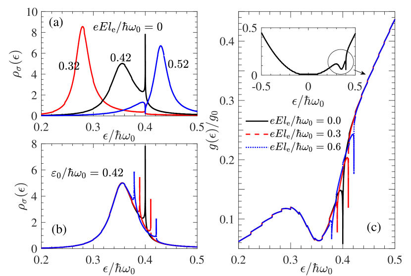
Figure 1: (a)-(b) The local DOSs $\rho_{\uparrow}(\epsilon)=\rho_{\downarrow}(\epsilon)$ at the impurity site and (c) the DOSs $g(\epsilon)$ for the disorder-averaged WSM as functions of energy $\epsilon$ of the itinerant electrons. The inset of (c) shows $g(\epsilon)$ vs $\epsilon$ for $eEl_{\mathrm{e}}=0$ and $\varepsilon_{0}/\hbar\omega_{0}=0.42$, where the region marked by the circle is replotted in (c) for different external electric fields. For convenience, we scale the energy and DOSs, respectively, with $\hbar\omega_{0}$ ($\sim 0.01$ eV) and $g_{0}=(\hbar\omega_{0})^{2}/4\pi^{2}(\hbar\upsilon_{\mathrm{F}})^{3}$, where $\omega_{0}=\upsilon_{\mathrm{F}}/\ell_{0}$ and $\ell_{0}=\sqrt{\hbar/e[B=1\text{ }\mathrm{Tesla}]}$. Here, we set (a) $eEl_{\mathrm{e}}=0$, $\varepsilon_{0}/\hbar\omega_{0}=(0.32,0.42,0.52)$ and (b)-(c) $\varepsilon_{0}/\hbar\omega_{0}=0.42$, $eEl_{\mathrm{e}}/\hbar\omega_{0}=(0,0.3,0.6)$. Other parameters are chosen as $\theta=0$, $\hbar\omega_{c}/\hbar\omega_{0}=0.1$, $E_{\mathrm{F}}/\hbar\omega_{0}=0.4$, $\gamma\equiv\hbar/\tau_{m}=0.05\hbar\omega_{0},t_{\sigma}=\hbar\omega_{0}$, $k_{B}T/\hbar\omega_{0}=10^{-7}$, $\Lambda/\hbar\omega_{0}=100$ and $U/\hbar\omega_{0}=1000.$

III Valley-dependent local equilibrium electron distribution function

When an external electric field $\mathbf{E}=E\hat{e}_{z}$ is applied, the electron distribution function will deviate from the equilibrium electron distribution function $f(\epsilon)=1/[1+e^{\beta(\epsilon-E_{\mathrm{F}})}]$, where $\beta=1/k_{B}T$. In the relaxation time approximation, the steady-state Boltzmann equation for the $\chi$ valley isDeng et al. (2019a, c)

$$e\mathbf{E}\cdot\bm{\upsilon}_{\alpha}^{\chi}\left(-\frac{\partial f_{\alpha}^{\chi}}{\partial\varepsilon_{\alpha}^{\chi}}\right)=-\frac{f_{\alpha}^{\chi}-f_{\chi}}{\tau_{\mathrm{intra}}}-\frac{f_{\alpha}^{\chi}-f_{g}}{\tau_{\mathrm{inter}}},$$ (16)

where $\bm{\upsilon}_{\alpha}^{\chi}=\hbar^{-1}\nabla_{\mathbf{k}}\varepsilon_{\alpha}^{\chi}$ is the group velocity, $f_{\chi}$ and $f_{g}$ represent, respectively, the local and global equilibrium electron distribution functions. The local equilibrium electron distribution function equals to statistically averaging $f_{\alpha}^{\chi}$ over quantum states around the local Fermi surface of valley $\chi$, i.e., $f_{\chi}=\langle f_{\alpha}^{\chi}\rangle_{\chi}$ with

$$\langle\cdots\rangle_{\chi}\equiv\frac{\int d\epsilon[-\partial_{\epsilon}f(\epsilon)]\sum_{\alpha}g_{\alpha}^{\chi}(\epsilon)(\cdots)}{\int d\epsilon[-\partial_{\epsilon}f(\epsilon)]\sum_{\alpha}g_{\alpha}^{\chi}(\epsilon)}$$ (17)

and $g_{\alpha}^{\chi}(\epsilon)=-\frac{1}{\pi}\operatorname{Im}(\frac{1}{\epsilon^{+}-\varepsilon_{\alpha}^{\chi}})$ is the momentum-resolved density of states (DOSs) for the WSM without impurity-WSM coupling. The global equilibrium electron distribution function $f_{g}$ can be calculated similarly, by summation over $\chi$ separately for the numerator and denominator in Eq. (17). Performing the local Fermi surface average on the both sides of Eq. (16) yields

$$eE\langle\upsilon_{\alpha,z}^{\chi}\rangle_{\chi}\left(-\frac{\partial f_{\chi}}{\partial\varepsilon_{\alpha}^{\chi}}\right)=-\frac{f_{\chi}-f_{g}}{\tau_{\mathrm{inter}}}.$$ (18)

Together with $f_{g}=(f_{\chi}+f_{-\chi})/2$, the local equilibrium electron distribution function can be finally obtained as

$$f_{\chi}=f(\varepsilon_{\alpha}^{\chi})-eE\langle\upsilon_{\alpha,z}^{\chi}\rangle_{\chi}\tau_{\mathrm{inter}}\left[-\frac{\partial f(\varepsilon_{\alpha}^{\chi})}{\partial\varepsilon_{\alpha}^{\chi}}\right],$$ (19)

in which we approximated $\partial_{\varepsilon_{\alpha}^{\chi}}f_{\chi}\simeq\partial_{\varepsilon_{\alpha}^{\chi}}f(\varepsilon_{\alpha}^{\chi})$. Within the framework of linear response, the valley-dependent local equilibrium electron distribution function can be expressed as $f_{\chi}(\varepsilon_{\alpha}^{\chi})=f(\varepsilon_{\alpha}^{\chi}+\Delta\mu_{\chi})$, where $\Delta\mu_{\chi}=eE\langle\upsilon_{\alpha,z}^{\chi}\rangle_{\chi}\tau_{\mathrm{inter}}$. In the absence of the magnetic field, $\langle\upsilon_{\alpha,z}^{\chi}\rangle_{\chi}=0$ and $\Delta\mu_{\chi}$ vanishes, while, if $B\neq 0$, we can obtain a nonzero $\Delta\mu_{\chi}=-\chi\Delta\mu$, where

$$\Delta\mu=eEl_{\mathrm{e}}\cos\theta\frac{1}{\int d\epsilon\left[-\partial_{\epsilon}f(\epsilon)\right]\varTheta(\epsilon)}$$ (20)

is the so-call chiral chemical potential due to the chiral anomaly and $l_{\mathrm{e}}=\upsilon_{\mathrm{F}}\tau_{\mathrm{inter}}$ is the intervalley relaxation length. Here, we note

$$\varTheta(\epsilon) \equiv\sum_{\alpha}g_{\alpha}^{\chi}(\epsilon)$$

$$=2\sum_{n=1}^{n_{c}}\operatorname{Im}[\frac{\epsilon}{\lambda_{n}(\epsilon^{+})}\frac{1}{\pi}\ln\frac{\lambda_{n}(\epsilon^{+})-\Lambda}{\lambda_{n}(\epsilon^{+})+\Lambda}]+1$$ (21)

for brevity, in which $\lambda_{n}(\epsilon)=\sqrt{\epsilon^{2}-2|n|(\hbar\omega_{c})^{2}}$ and $\Lambda$ is a high-energy cutoff for the linear dispersion.

Replacing the momentum summation in Eq. (14) by an integral, the self-energies can be further reduced to be $\Sigma_{\sigma}^{r}=-i\Gamma_{\sigma}(\epsilon)$, $\tilde{\Sigma}_{\sigma}^{r}=-i\left[\Gamma_{\bar{\sigma}}(\epsilon_{\sigma})+\Gamma_{\bar{\sigma}}(\epsilon_{U})\right]$ and

$$\Sigma_{\sigma}^{<} =-\frac{i}{2}\left[\Gamma_{\bar{\sigma}}(\epsilon_{\sigma})+\Gamma_{\bar{\sigma}}(\epsilon_{U})\right]$$

$$-\frac{1}{2\pi}\sum_{\chi}\Gamma_{\bar{\sigma}}(\epsilon_{\sigma})\psi(\frac{1}{2}+\frac{\epsilon_{\sigma}-\chi\Delta\mu-E_{\mathrm{F}}}{2\pi ik_{B}T})$$

$$+\frac{1}{2\pi}\sum_{\chi}\Gamma_{\bar{\sigma}}(\epsilon_{U})\psi(\frac{1}{2}+\frac{\epsilon_{U}+\chi\Delta\mu+E_{\mathrm{F}}}{2\pi ik_{B}T}),$$ (22)

where $\psi(x)$ is the digamma function and $\Gamma_{\sigma}(\epsilon)=\sum_{\alpha}\pi|t_{\alpha\chi\sigma}|^{2}g_{\alpha}^{\chi}(\epsilon)\theta(\Lambda^{2}-\epsilon^{2})$ is the linewidth function of the impurity level due to the WSM-impurity coupling.

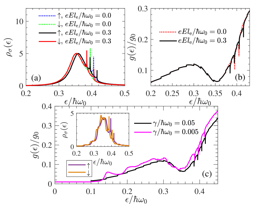
Figure 2: The DOSs (a) $\rho_{\sigma}(\epsilon)$ and (b)-(c) $g(\epsilon)$ as functions of $\epsilon$ for a finite Zeeman field $\Delta/\hbar\omega_{0}=0.0025$ at the impurity sites, where the inset of (c) shows $\rho_{\sigma}(\epsilon)$ vs $\epsilon$ for $\gamma/\hbar\omega_{0}=0.005$. The parameters are set as (a)-(b) $\gamma/\hbar\omega_{0}=0.05$, $eEl_{\mathrm{e}}/\hbar\omega_{0}=(0,0.3)$, and (c) $eEl_{\mathrm{e}}/\hbar\omega_{0}=0.3$, $\gamma/\hbar\omega_{0}=(0.05,0.005)$. Other parameters are chosen the same as Fig. 1(c).

IV Chiral anomaly modulated Kondo effect

In the following, we would consider the deep Coulomb blockade regime, i.e., $U\rightarrow\infty$, in which we can further reduce the impurity Green’s function to a simple form

$$G_{d\sigma\sigma}^{r}(\epsilon)=\frac{1-\langle n_{\bar{\sigma}}\rangle}{\epsilon-\varepsilon_{\sigma}-\Sigma_{\sigma}^{r}-\Sigma_{\sigma}^{<}}.$$ (23)

The spin-dependent electron DOSs at the impurity site, defined as $\rho_{\sigma}(\epsilon)=-\mbox{Im}\left[G_{d\sigma\sigma}^{r}(\epsilon)\right]/\pi$, is plotted in Figs. 1(a) and (b). From Fig. 1(a), we can see that there appears a Lorenz peak around the renormalized impurity level $\tilde{\varepsilon}_{\sigma}=\varepsilon_{\sigma}+\operatorname{Re}(\Sigma_{\sigma}^{r}+\Sigma_{\sigma}^{<})$, which characterizes the charge fluctuation between the WSM host and impurity. With the impurity level approaching the Fermi level, an additional sharp peak emerges to decorate the Lorenz resonance peak when the temperature is below a critical value $T_{K}$. This sharp peak, in fact, is attributable to the Kondo effect, which has been widely studied in varied systemsWang et al. (2007); Feng et al. (2010); Tran and Kim (2010); Zhu and Berakdar (2011); Mitchell et al. (2013); Orignac and Burdin (2013); Deng et al. (2016); Zheng et al. (2016); Mitchell and Fritz (2015); Sun et al. (2015); Ma et al. (2018); Li et al. (2018); Lü et al. (2019). The Kondo peak comes from the spin fluctuation at the Fermi level, which apart from the temperature, is very sensitive to the location of the Fermi level. In the presence of nonorthogonal electric and magnetic fields, the WSM will exhibit the chiral anomaly, which creates a chirality population imbalance between the Weyl valleys. The resulting chiral chemical potential will shift the local Fermi levels of the two paired Weyl valleys in opposite directions in energy, as shown by Eq. (19). Consequently, in response to the chiral chemical potential, a single Kondo peak, as seen from Fig. 1(b), will split into a pair of peaks residing at the two sides of $\epsilon=E_{\mathrm{F}}$, whose energy spacing is equal to twice of the chiral chemical potential. This scenario is similar to that in Ref. Li et al. (2018). The electron exchange rate $1/\tau_{\varphi}$ between the WSM and impurity increases as $\epsilon$ approaches the impurity level, so that the DOSs of the WSM $g(\epsilon)=-\mbox{Im}\sum_{\alpha}\mathrm{Tr}\left[G_{\alpha,\alpha}^{\chi,\chi}(\epsilon)\right]/\pi$, in response to $\rho_{\sigma}(\epsilon)$, exhibits an inverse Lorenz structure, and the Kondo peak is also observable, as indicated in the inset of Fig. 1(c), where a sharp dip exists at the Fermi level. With the electric field turned on, a single sharp dip, due to the chiral anomaly, develops into a pair of sharp dips distributed symmetrically with respect to the Fermi level, as shown in Fig. 1(c).

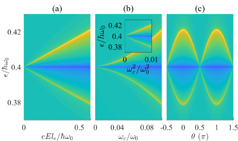
Figure 3: Evolution of (a) $\Delta\rho_{\sigma}(E)=[\rho_{\sigma}(E)-$ $\rho_{\sigma}(E=0)]/\rho_{\sigma}(E=0)$ with $\theta=0$ and $\hbar\omega_{c}/\hbar\omega_{0}=0.1$, (b) $\Delta\rho_{\sigma}(B)=[\rho_{\sigma}(B)-$ $\rho_{\sigma}(B=0)]/\rho_{\sigma}(B=0)$ with $\theta=0$ and $eEl_{\mathrm{e}}/\hbar\omega_{0}=0.6$, and (c) $\Delta\rho_{\sigma}(\theta)=[\rho_{\sigma}(\theta)-$ $\rho_{\sigma}(\theta=\pi/2)]/\rho_{\sigma}(\theta=\pi/2)$ with $\hbar\omega_{c}/\hbar\omega_{0}=0.1$ and $eEl_{\mathrm{e}}/\hbar\omega_{0}=0.6$, where the values of $\Delta\rho_{\sigma}$ are denoted by the filled colors. The data of (b) is replotted in the inset to show the $B$-linear ($\omega_{c}^{2}$) dependence of the chiral chemical potential. Other parameters are the same as Fig. 1(c).

The appearance of the Kondo peaks, resembling the scenario of an impurity deposited in graphene or on the surface of topological insulatorsZhu and Berakdar (2011); Deng et al. (2016), is attributable to the singularity of the impurity Green’s function at the Fermi level. Since the real part of the digamma function $\psi(\frac{1}{2}+\frac{\epsilon_{\sigma}-\chi\Delta\mu-E_{\mathrm{F}}}{2\pi ik_{B}T})$ develops a sharp peak at $\epsilon_{\sigma}-\chi\Delta\mu=E_{\mathrm{F}}$ when the temperature is lower than the Kondo temperature $T_{K}$, there always exists a solution for $\epsilon-\varepsilon_{\sigma}-\operatorname{Re}(\Sigma_{\sigma}^{r}+\Sigma_{\sigma}^{<})=0$ at $\epsilon_{\sigma}=E_{\mathrm{F}}+\chi\Delta\mu$, which contributes a singularity to the impurity Green’s function. Accordingly, the Kondo peaks in fact develop at $\epsilon=E_{\mathrm{F}}+\chi\Delta\mu+\sigma\Delta$, where $\Delta=\varepsilon_{\uparrow}-\varepsilon_{\downarrow}$ is the Zeeman splitting energy of the impurity level. As it shows, the Zeeman field on the impurity site can also result in splitting of the Kondo peak, which is also reported in Ref. Li et al. (2018). However, in this situation, if $\Delta\mu=0$, the Zeeman field just shifts the Kondo peaks for the two spin sectors toward different directions in energy, as shown by the dotted lines in Fig. 2(a), so that each spin component still contains only one Kondo peak. Meanwhile, the Lorenz resonance peaks for the two spin components would separate from each other because of broken spin degeneracy of the impurity level. Differently, the chiral anomaly will induce a pair of Kondo peaks for both spin components, as seen from Fig. 1(b) and Fig. 2(a), and, if $\Delta=0$, the DOSs remain identical for the two spin species. As indicated by Fig. 2(b), including both the chiral anomaly and Zeeman effect on the impurity sites, the two Kondo dips (red-dotted line) for the WSM would split into four dips (dark-solid line). Due to the LL quantization, the DOSs of the WSM may exhibit quantum oscillations, which depends on the relative magnitudes of the spacing $\Delta_{n}=\sqrt{2}\hbar\omega_{c}(\sqrt{|n+1|}-\sqrt{|n|})$ and impurity-induced broadening $\gamma\equiv\hbar/\tau_{m}$ of the LLs. The quantum oscillations are resolvable only when $\Delta_{n}$ is much greater than $\gamma$, and so it is expected that the quantum oscillations in the LNMR are sensitive to the impurity scattering, especially for weak magnetic fields. However, as shown by Fig. 2(c), the Kondo peaks are less sensitive to the broadening of the LLs. As seen from the inset of Fig. 2(c), the quantum oscillations also can be reflected in the Lorenz peaks of the impurity DOSs.

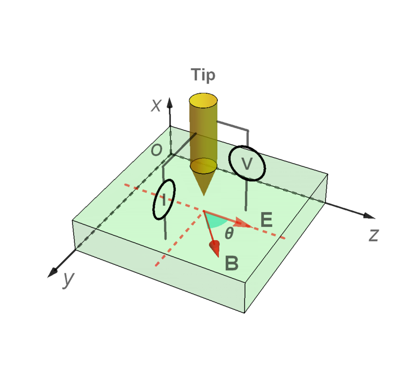
Figure 4: Schematics of the device for point contact measurementWang et al. (2016, 2017b, 2017c), where a STM tip (brown) is attached to the top of a doped WSM slap (cyan).

To extract information of the chiral chemical potential, we plot $\Delta\rho_{\sigma}(E)=[\rho_{\sigma}(E)-$ $\rho_{\sigma}(E=0)]/\rho_{\sigma}(E=0)$ in Fig. 3(a), $\Delta\rho_{\sigma}(B)=[\rho_{\sigma}(B)-$ $\rho_{\sigma}(B=0)]/\rho_{\sigma}(B=0)$ in Fig. 3(b) and $\Delta\rho_{\sigma}(\theta)=[\rho_{\sigma}(\theta)-$ $\rho_{\sigma}(\theta=\pi/2)]/\rho_{\sigma}(\theta=\pi/2)$ in Fig. 3(c), respectively in the $E$-$\epsilon$, $B$-$\epsilon$ and $\theta$-$\epsilon$ parameter spaces, through which the background DOSs can be subtracted to highlight the locations of the Kondo peaks. The evolution of the energy positions of the Kondo peaks are demonstrated by the yellow regions. The dark blue lines along $\epsilon/\hbar\omega_{0}=0.4$ correspond to the Kondo peaks for the case of vanishing chiral chemical potential, which locates the Fermi energy. As seen from Fig. 3(a), for fixed $B$ and $\theta$, the Kondo peaks will deviate from the Fermi level, with the deviation $|\Delta\epsilon|\propto E$. For fixed $E$ and $\theta$, $|\Delta\epsilon|\propto(\hbar\omega_{c})^{2}\sim B$, while for fixed $B$ and $E$, $|\Delta\epsilon|\propto\cos\theta$, as indicated in Figs. 3(b) and (c). Similar patterns also emerge in the DOSs of the WSM. This implies that the separation of the Kondo peaks is proportional to $\mathbf{E}\cdot\mathbf{B}$, which demonstrates the chiral anomaly origin of the splitting of the Kondo peaks. Therefore, the Kondo effect in magnetic and electric field driven WSMs can capture the characteristics of the chiral anomaly, and the observation of the electrically tunable Kondo effect can provide an exclusive evidence for the emergence of the chiral anomaly in WSMs.

V Discussion and conclusion

To date, experiments about the chiral-anomaly-modulated Kondo effect are still absent. In experiment, the chiral anomaly can be detected by using point contact spectroscopy measurementsWang et al. (2016, 2017b, 2017c), as depicted in Fig. 4. The setup consists of a doped WSM slap (cyan) and a scanning tunneling microscopy (STM). The electric and magnetic fields are applied in the $y$-$z$ plane to induce the chiral chemical potential and the STM tip is attached to the top of the WSM slap to measure the differential conductance between the STM and WSM. The chemical potential of the WSM can be tuned by a gate voltage, which is not shown. For a fixed electric and magnetic field, as the chemical potential of the WSM varies, the differential conductance will develop a sharp peak when a local Fermi energy encounters the renormalized impurity level. The energy locations of the Kondo peaks correspond to the sharp peaks of the differential conductance, whose spacing reflects the chiral chemical potential.

In conclusion, we have investigated the Kondo effect in magnetic and electric field driven WSMs. It is found that, due to the chiral anomaly, unequal local Fermi levels can be established between the paired Weyl valleys, and so lead to splitting of the Kondo peaks. The external field dependent chiral chemical potential makes the Kondo peaks electrically tunable. The electrically tunable Kondo peaks is unique to the chiral anomaly and thus can serve as a direct measurement of the chiral anomaly. The Kondo effect is less sensitive to the disorder effect than transport signals, so that the chiral anomaly survives for relatively weak magnetic fields.

VI acknowledgements

This work was supported by the National Natural Science Foundation of China under Grants No. 11904107 (M.X.D), 11874016 (R.Q.W), and 11804130 (W.L), by the Guangdong NSF of China under Grant No. 2020A1515011566 (M.X.D) and the Key Program for Guangdong NSF of China under Grant No. 2017B030311003, GDUPS(2017) and by the projects funded by South China Normal University under Grant No. 671215 and 8S0532.

References

- Armitage et al. (2018) N. P. Armitage, E. J. Mele, and A. Vishwanath, Rev. Mod. Phys. 90, 015001 (2018).
- Zhang et al. (2016) C.-L. Zhang, S.-Y. Xu, I. Belopolski, Z. Yuan, Z. Lin, B. Tong, G. Bian, N. Alidoust, C.-C. Lee, S.-M. Huang, T.-R. Chang, G. Chang, C.-H. Hsu, H.-T. Jeng, M. Neupane, D. S. Sanchez, H. Zheng, J. Wang, H. Lin, C. Zhang, H.-Z. Lu, S.-Q. Shen, T. Neupert, M. Zahid Hasan, and S. Jia, Nat. Commun. 7, 10735 (2016).
- Liu et al. (2014) Z. K. Liu, B. Zhou, Y. Zhang, Z. J. Wang, H. M. Weng, D. Prabhakaran, S.-K. Mo, Z. X. Shen, Z. Fang, X. Dai, Z. Hussain, and Y. L. Chen, Science 343, 864 (2014).
- Xiong et al. (2015) J. Xiong, S. K. Kushwaha, T. Liang, J. W. Krizan, M. Hirschberger, W. Wang, R. J. Cava, and N. P. Ong, Science 350, 413 (2015).
- Zhang et al. (2017) C. Zhang, E. Zhang, W. Wang, Y. Liu, Z.-G. Chen, S. Lu, S. Liang, J. Cao, X. Yuan, L. Tang, Q. Li, C. Zhou, T. Gu, Y. Wu, J. Zou, and F. Xiu, Nat. Commun. 8, 13741 (2017).
- Wang et al. (2017a) C. M. Wang, H.-P. Sun, H.-Z. Lu, and X. C. Xie, Phys. Rev. Lett. 119, 136806 (2017a).
- Zhang et al. (2018) D.-W. Zhang, Y.-Q. Zhu, Y. X. Zhao, H. Yan, and S.-L. Zhu, Advances in Physics 67, 253 (2018).
- Deng et al. (2019a) M.-X. Deng, G. Y. Qi, R. Ma, R. Shen, R.-Q. Wang, L. Sheng, and D. Y. Xing, Phys. Rev. Lett. 122, 036601 (2019a).
- Li et al. (2019) X.-S. Li, C. Wang, M.-X. Deng, H.-J. Duan, P.-H. Fu, R.-Q. Wang, L. Sheng, and D. Y. Xing, Phys. Rev. Lett. 123, 206601 (2019).
- Zhang et al. (2015) D.-W. Zhang, S.-L. Zhu, and Z. D. Wang, Phys. Rev. A 92, 013632 (2015).
- Zheng et al. (2019) Z. Zheng, Z. Lin, D.-W. Zhang, S.-L. Zhu, and Z. D. Wang, Phys. Rev. Research 1, 033102 (2019).
- Volovik (2003) G. E. Volovik, The universe in a helium droplet, Vol. 117 (Oxford University Press on Demand, 2003).
- Yang and Nagaosa (2014) B.-J. Yang and N. Nagaosa, Nat. Commun. 5, 4898 (2014).
- Gorbar et al. (2015) E. V. Gorbar, V. A. Miransky, I. A. Shovkovy, and P. O. Sukhachov, Phys. Rev. B 91, 121101 (2015).
- Kargarian et al. (2016) M. Kargarian, M. Randeria, and Y.-M. Lu, Proceedings of the National Academy of Sciences 113, 8648 (2016).
- Wan et al. (2011) X. Wan, A. M. Turner, A. Vishwanath, and S. Y. Savrasov, Phys. Rev. B 83, 205101 (2011).
- Ali et al. (2014) M. N. Ali, J. Xiong, S. Flynn, J. Tao, Q. D. Gibson, L. M. Schoop, T. Liang, N. Haldolaarachchige, M. Hirschberger, N. Ong, and R. Cava, Nature 514, 205 (2014).
- Shekhar et al. (2015) C. Shekhar, A. K. Nayak, Y. Sun, M. Schmidt, M. Nicklas, I. Leermakers, U. Zeitler, Y. Skourski, J. Wosnitza, Z. Liu, Y. Chen, W. Schnelle, H. Borrmann, Y. Grin, C. Felser, and B. Yan, Nat. Phys. 11, 645 (2015).
- Parameswaran et al. (2014) S. A. Parameswaran, T. Grover, D. A. Abanin, D. A. Pesin, and A. Vishwanath, Phys. Rev. X 4, 031035 (2014).
- Deng et al. (2017) M.-X. Deng, W. Luo, R.-Q. Wang, L. Sheng, and D. Y. Xing, Phys. Rev. B 96, 155141 (2017).
- Huang et al. (2015) X. Huang, L. Zhao, Y. Long, P. Wang, D. Chen, Z. Yang, H. Liang, M. Xue, H. Weng, Z. Fang, X. Dai, and G. Chen, Phys. Rev. X 5, 031023 (2015).
- Liang et al. (2018) S. Liang, J. Lin, S. Kushwaha, J. Xing, N. Ni, R. J. Cava, and N. P. Ong, Phys. Rev. X 8, 031002 (2018).
- Neupane et al. (2014) M. Neupane, S.-Y. Xu, R. Sankar, N. Alidoust, G. Bian, C. Liu, I. Belopolski, T.-R. Chang, H.-T. Jeng, H. Lin, A. Bansil, F. Chou, and M. Z. Hasan, Nat. Commun. 5, 3786 (2014).
- Li et al. (2015) C.-Z. Li, L.-X. Wang, H. Liu, J. Wang, Z.-M. Liao, and D.-P. Yu, Nat. Commun. 6, 10137 (2015).
- Lu and Shen (2015) H.-Z. Lu and S.-Q. Shen, Phys. Rev. B 92, 035203 (2015).
- Deng et al. (2019b) M.-X. Deng, Y.-Y. Yang, W. Luo, R. Ma, C.-Y. Zhu, R.-Q. Wang, L. Sheng, and D. Y. Xing, Phys. Rev. B 100, 235105 (2019b).
- Deng et al. (2019c) M.-X. Deng, H.-J. Duan, W. Luo, W. Y. Deng, R.-Q. Wang, and L. Sheng, Phys. Rev. B 99, 165146 (2019c).
- Mitchell and Fritz (2015) A. K. Mitchell and L. Fritz, Phys. Rev. B 92, 121109 (2015).
- Sun et al. (2015) J.-H. Sun, D.-H. Xu, F.-C. Zhang, and Y. Zhou, Phys. Rev. B 92, 195124 (2015).
- Ma et al. (2018) D. Ma, H. Chen, H. Liu, and X. C. Xie, Phys. Rev. B 97, 045148 (2018).
- Li et al. (2018) L. Li, J.-H. Sun, Z.-H. Wang, D.-H. Xu, H.-G. Luo, and W.-Q. Chen, Phys. Rev. B 98, 075110 (2018).
- Lü et al. (2019) H.-F. Lü, Y.-H. Deng, S.-S. Ke, Y. Guo, and H.-W. Zhang, Phys. Rev. B 99, 115109 (2019).
- Wang et al. (2007) R.-Q. Wang, Y.-Q. Zhou, B. Wang, and D. Y. Xing, Phys. Rev. B 75, 045318 (2007).
- Feng et al. (2010) X.-Y. Feng, W.-Q. Chen, J.-H. Gao, Q.-H. Wang, and F.-C. Zhang, Phys. Rev. B 81, 235411 (2010).
- Tran and Kim (2010) M.-T. Tran and K.-S. Kim, Phys. Rev. B 82, 155142 (2010).
- Zhu and Berakdar (2011) Z.-G. Zhu and J. Berakdar, Phys. Rev. B 84, 165105 (2011).
- Mitchell et al. (2013) A. K. Mitchell, D. Schuricht, M. Vojta, and L. Fritz, Phys. Rev. B 87, 075430 (2013).
- Orignac and Burdin (2013) E. Orignac and S. Burdin, Phys. Rev. B 88, 035411 (2013).
- Deng et al. (2016) M.-X. Deng, R.-Q. Wang, W. Luo, L. Sheng, B. G. Wang, and D. Y. Xing, New J. Phys. 18, 093040 (2016).
- Datta (1997) S. Datta, Electronic transport in mesoscopic systems (Cambridge University Press, 1997).
- Mahan (2013) G. D. Mahan, Many-particle physics (Springer Science & Business Media, 2013).
- Zheng et al. (2016) S.-H. Zheng, R.-Q. Wang, M. Zhong, and H.-J. Duan, Scientific Reports 6, 36106 (2016).
- (43) See the Supplemental Material for a detail derivation of the retarded Green’s functions for the disorder WSMs and the Anderson impurities, and estimation for the momentum-relaxation times.
- Deng et al. (2019d) M.-X. Deng, G. Y. Qi, W. Luo, R. Ma, R.-Q. Wang, R. Shen, L. Sheng, and D. Y. Xing, Phys. Rev. B 99, 085106 (2019d).
- Wang et al. (2016) H. Wang, H. Wang, H. Liu, H. Lu, W. Yang, S. Jia, X.-J. Liu, X. C. Xie, J. Wei, and J. Wang, Nature Materials 15, 38 (2016).
- Wang et al. (2017b) S. Wang, B.-C. Lin, A.-Q. Wang, D.-P. Yu, and Z.-M. Liao, Advances in Physics: X 2, 518 (2017b).
- Wang et al. (2017c) H. Wang, H. Wang, Y. Chen, J. Luo, Z. Yuan, J. Liu, Y. Wang, S. Jia, X.-J. Liu, J. Wei, and J. Wang, Science Bulletin 62, 425 (2017c).