Comparison of the Planck 2018 CMB polarization maps in the BICEP2/Keck region

Abstract

We examine the statistical properties of polarization maps from Planck 2018 within the patch of sky observed by the BICEP2/Keck experiment using the one point distribution function (1PDF), skewness, and kurtosis statistics. Our analysis is performed for the Q and U Stokes parameters and for the corresponding E- and B-modes of the CMB signals. We extend our analysis by studying the correlations between CMB polarization maps and residual maps (the difference between the full signal and the CMB map) for the frequency range of 100–217 GHz with both the Q/U and E/B approaches. Although all the CMB maps reveal almost Gaussian statistical properties for Q/U and E/B domains, we have detected very significant anomalies for cross-correlations with residuals at 100 GHz at the level of $3.7\sigma$ for the Commander map and $5.2\sigma$ for NILC, for both the Q and U parameters. Using the NILC–Commander difference, which does not contain a cosmological signal, we find a sub-dominant non-Gaussian component in Q skewness and kurtosis at the level of $4.3\sigma$ and $10\sigma$, respectively. For the B-mode we have found a very high level of cross-correlation (0.63–0.69) between the NILC/Commander maps and the 143 GHz total signal, which cannot be associated with the cosmological component. These strong deviations suggest that remnants of foregrounds, systematic effects, and component separation exist in the 2018 Planck CMB polarization maps in the BICEP2 sky area, which is far away from the Galactic plane. Our analysis also demonstrates the preferability of the Q/U domain over E/B for determination of the statistical properties of the derived CMB signals, due to non-locality of the transition Q/U $\rightarrow$ E/B.

1 Introduction

The next generation of CMB experiments [1, 2, 3, 4, 5, 6] is dedicated to one of the most important tasks of fundamental physics: the detection of cosmological gravitational waves. To achieve this goal, it is necessary to detail existing models of polarization foregrounds, especially for the B-mode. For this it seems important to us to use prior experience, including the BICEP2/Keck Array experiment [7](hereafter, the BICEP2 zone) in combination with Planck 2018 CMB products [8], in order to understand in which direction we should focus both in the modeling of foregrounds and in the methods for extracting the cosmological signal. In this article, we analyze the properties of four CMB polarization maps, SMICA, NILC, Commander, and SEVEM, from the Planck 2018 data release in the sky region of the BICEP2 experiment in two main ways. First of all, we will be interested in the Pearson cross-correlation coefficient [9] between CMB maps and residuals (the difference between the full signal and the CMB), which should to be at the level of chance correlations if the CMB does not contain residuals from foregrounds and systematics. Secondly, we will study the distribution function (1PDF, skewness and kurtosis) for CMB products in the BICEP2 zone in order to understand how the remnants of foregrounds and systematics deviate these distributions from Gaussian expectations.

The non-triviality of using this combined approach is dictated by following circumstances. Usually, Gaussian or non-Gaussian, the derived CMB maps have specific Gaussian signs of the primordial cosmological signal and its contamination by the remnants of foregrounds and systematics [10]. However, the BICEP2 zone is located far from the Galactic plane, and the non-Gaussianity of foregrounds is no longer their characteristic feature. As shown in [11, 12], the deviation of the full-sky signal for the skewness and kurtosis statistics does not exceed 2 standard deviations for the 353 GHz sky map. Therefore, the test for cross-correlation between the derived CMB signal and relevant residuals becomes very important for understanding the level of contamination.

The main idea of our tests is that Planck 2018 CMB products (SMICA, NILC, Commander and SEVEM) are derived from the full sky analysis with different kind of masks and they based on optimisation of different functionals under various assumptions  [13]. Subtraction of the mean values of these functionals makes the methods globally non-local. We have two additional tasks among others:

1. To understand the properties of these polarisation CMB maps in the BICEP2 domain, which lies far away from the Galactic masks.

2. To compare them with local ILC map [14], derived just from BICEP2 domain for all 30–353 GHz total maps. We will perform our analysis on the Q and U components of the Stokes parameters, and look at the corresponding E and B components [15, 16, 17]. We use $N_{\mathrm{side}}=256$ and $1^{o}$ Gaussian beam smoothing, focusing on the first 100–200 multipoles.

Working with the Q and U maps, we can apply different statistics for amplitudes, making the corresponding statistics very informative. We will show that tests of non-Gaussianity of the E and B maps without the Q and U components can produce misleading effects.

The outline of the paper is the following. In section 2 we will describe statistical characteristics of the Q and U parameters for the Planck 2018 CMB maps, focusing on 1PDF, skewness, and kurtosis statistics in the BICEP2 zone. Here we will introduce the residuals of the total signal as a difference between the 100–217 GHz frequency maps and the SMICA, NILC, Commander and SEVEM maps. For comparison, we will include in the analysis our ILC map (local ILC), derived just from the 30–353 GHz signal in BICEP2 domain. Section 3 is devoted to the same analysis of the statistical properties of the polarization maps as for the Q and U domain, but for the corresponding E- and B-modes. Due to the very small fraction of the sky occupied by the BICEP2 zone, we have applied recycling E/B-leakage correction, proposed in [18, 19]. In Section 4 we investigate the skewness and kurtosis statistics for E- and B-modes of polarisation. We summarise our results in the Conclusion.

2 Planck 2018 CMB products in the BICEP2 region

In this section we compare the polarized CMB maps, SMICA, NILC, Commander, and SEVEM, from the Planck 2018 data release. These maps are derived from a masked full sky analysis, which we then restrict to the BICEP2 region, shown in figure 1. We will focus on the varying statistical properties of these maps, which reflect different methods of separating foregrounds from the primordial signal.

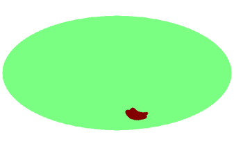
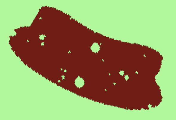
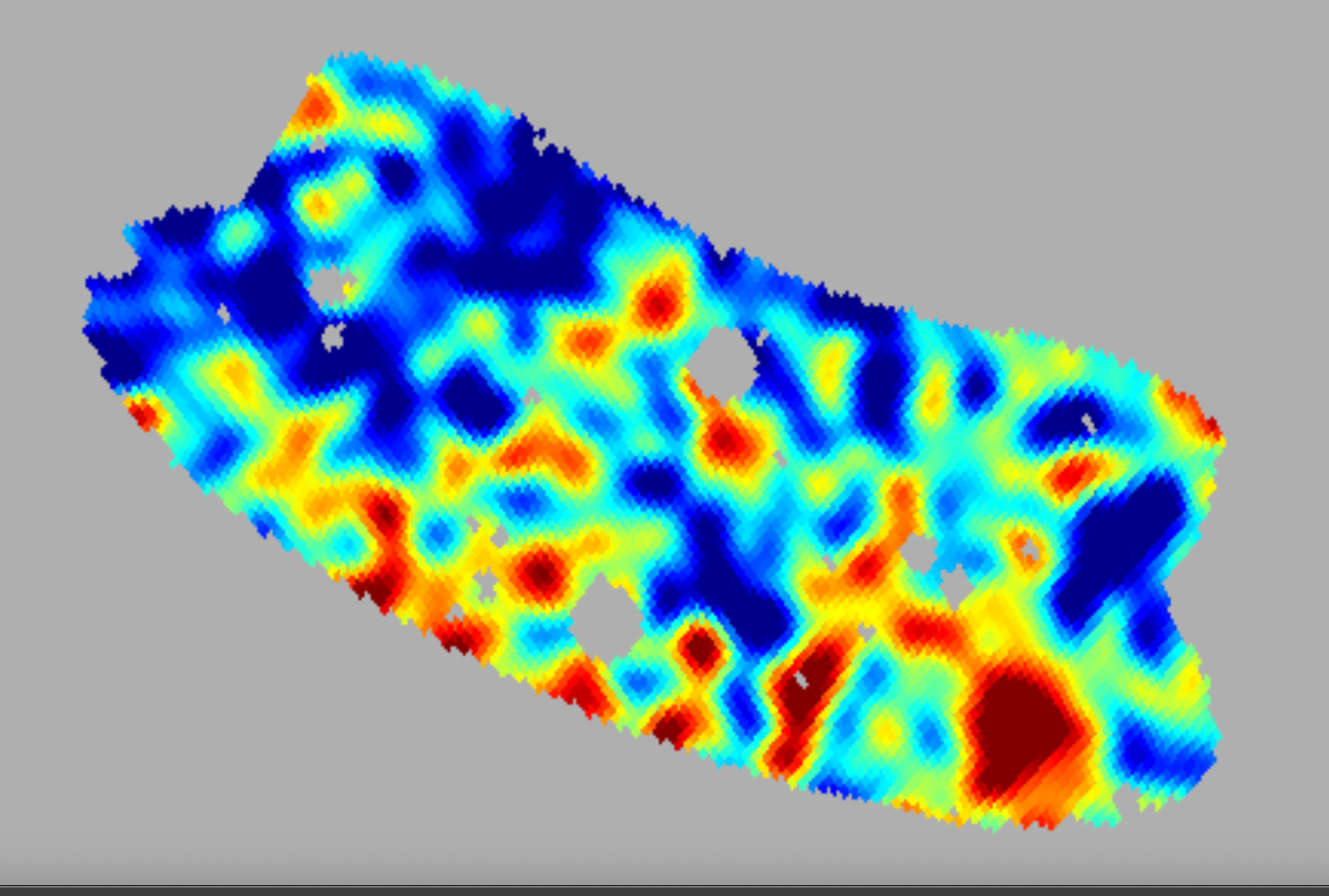
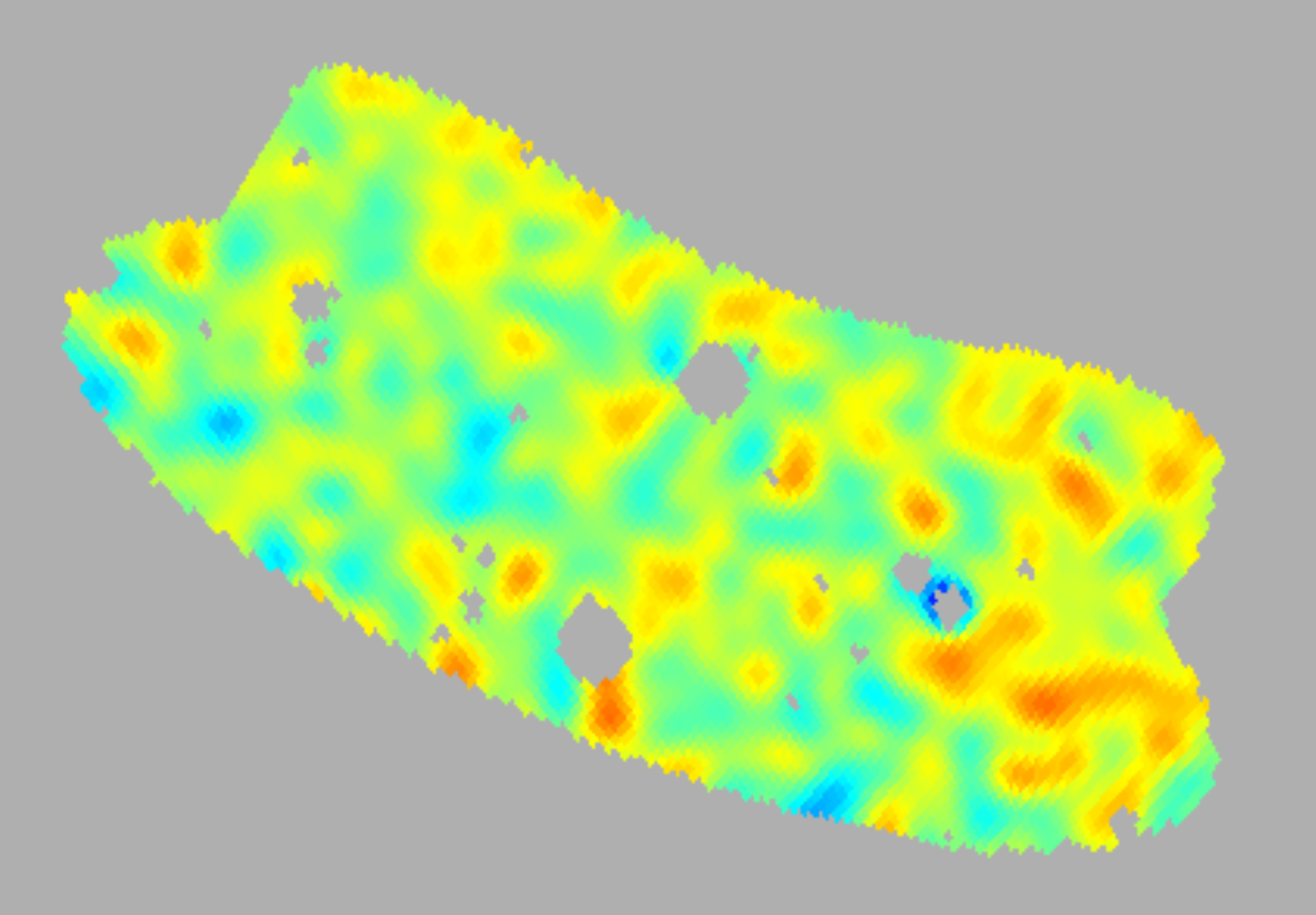
Figure 1: Upper panels: the BICEP2 zone and the Planck point sources mask which define the region under investigation. Lower left: the Commander map in this region. Lower right: The difference Commander$-$NILC map. Both the lower panels are for the temperature anisotropy. The color scale of the maps is $-100$ to $+100\mu$K.

We will add to our analysis the ILC map derived by us from the Planck 2018 30-353 GHz maps. The ILC coefficients are computed using the convenient solution given in [14]. All these maps are smoothed by a $1^{\circ}$ FWHM Gaussian beam.

In figure 1, the BICEP2 region is presented with implementation of the Union mask in that region for point-like sources. For illustration of the method we plot in that figure the temperature anisotropy maps for Commander and the difference between Commander and NILC maps. Both these maps, Commander and NILC, are characterised by very high signal-to-noise-ratio, and if they are Gaussian, the difference between them represents the residuals of the foregrounds and instrumental noise.

2.1 Asymmetry of distributions

As a first step of our analysis, in figure 2 we show the distribution function (histogram) of counts with given amplitudes of the Q and U components for the five maps in the BICEP2 zone. The variation of these distributions from each other is pronounced for Q but more stable for U.

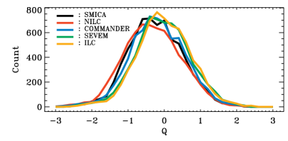
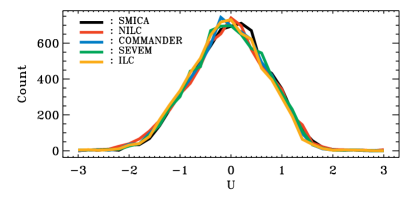
Figure 2: The histograms of the Q and U Stokes parameters (left and right) of the regions in figure 1 for the CMB maps.

The first test that can be applied for these histograms is the analysis of skewness and kurtosis. We will characterise the departure of these characteristics from Gaussian realisations in terms of standard deviations. For that we will generate $10^{3}$ Gaussian realisations in order to estimate the variance of distribution $\sigma$. Then in table 1 we present the corresponding significance of non-Gaussian features of distribution in terms of $\sigma$.

Input	Q skewness	Q kurtosis	U skewness	U kurtosis
SMICA	0.7	0.4	1.8	0.4
NILC	0.3	0.3	1.0	1.2
Commander	0.3	1.4	1.4	0.3
SEVEM	0.2	0.9	1.5	0.1
ILC	0.2	1.4	1.3	0.5

Table 1: The significances (multiples of $\sigma$ of estimator in the Gaussian case) of the skewness and kurtosis of the Q and U Stokes parameters for various maps.

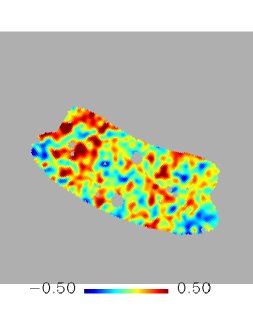
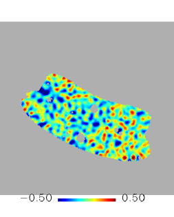
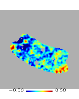
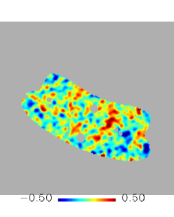
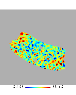
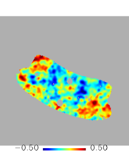
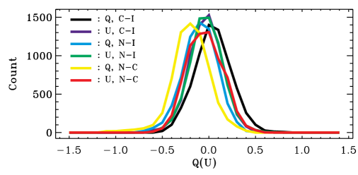
Figure 3: The differences of the Commander–ILC (left), NILC–ILC (middle) and Commander–NILC (right) maps in the BICEP2 zone for the Q and U Stokes parameters (upper-lower), and the histograms of them (bottom panel). The color scale corresponds to $-0.5$ to $0.5$ mK. From the top to the bottom: Commander–ILC, NILC–ILC and NILC–Commander.

As it is seen from table 1, the deviation from Gaussianity does not exceed $0.7\sigma$ for skewness and $1.4\sigma$ for kurtosis for Q, and $1.8\sigma$ and $1.2\sigma$ for U for all the CMB products in the BICEP2 zone.

At first glance, based on these estimators, all the Planck 2018 CMB products are in agreement with theoretical predictions and all the maps evenly well represent the properties of the primordial CMB signal in the BICEP2 domain. However, we should not forget that transition from Q and U Stokes parameters to E and B components is characterised by very strong differences in the power spectrum of these last components $C_{E}(l)$ and $C_{B}(l)$. As a standard prediction for the primordial CMB we can safely adopt $C_{B}(l)\ll C_{E}(l)$ for all tensor-to-scalar ratios $r\ll 1$. That means that skewness and kurtosis test is simply not sensitive enough for any conclusions about Gaussianity of the derived E and B- components. In addition, we should take under consideration potential Gaussianity of the foregrounds [11, 12] in the BICEP2 domain, located far away from the Galactic plane. Let’s clarify that issue with the following toy model.

Suppose that all the CMB products can be written as a linear combination of the primordial signal $S_{cmb}$, the instrumental noise $n_{i}$, and the residuals of systematic and foregrounds removal $S^{(i)}_{r}$:

$$S_{i}=S_{cmb}+S^{(i)}_{r}+n_{i}$$ (2.1)

where index $i$ marks the SMICA, NILC, Commander, SEVEM, and ILC maps correspondingly. The primordial CMB component $S_{cmb}$ obeys Gaussian statistics for all maps. The same statistical properties can be assumed for the instrumental noise, while for foreground residuals (see, however [11, 12]) and systematics we may expect departure from Gaussianity. From eq. (2.1) one can see two potential sources of Gaussianity, $S_{cmb}$ and $n_{i}$. Thus, if we will focus on the differences $M_{i,j}=S_{i}-S_{j}$, then the CMB component will not affect the statistics of these maps. Obviously, the difference of the noises $n_{i}-n_{j}$ will still affect the non-Gaussianity of the foregrounds and systematics, but the CMB contribution can be greatly reduced. In the next section we will focus on investigation of the statistical properties of the maps of differences.

2.2 Cross-correlations with residuals

For estimation of possible contamination of the derived CMB products, we use the Pearson’s coefficient of cross-correlation between any two signals, $A$ and $B$, defined as follows:

$$C_{A,B}=\frac{\sum_{i}a_{i}b_{i}}{\sigma_{A}\sigma_{B}}\hskip 14.22636pta_{i}=A_{i}-\langle A_{i}\rangle,b_{i}=B_{i}-\langle B_{i}\rangle$$

$$\sigma_{G}=\left(\sum_{i}(G_{i}-\langle G_{i}\rangle)^{2}\right)^{\frac{1}{2}},\hskip 5.69046ptG=A,B$$ (2.2)

where $i$ indicates the pixels in the map under consideration, and

$$\langle G_{i}\rangle=\sum_{i}G_{i}.$$ (2.3)

Suppose that signal $b$ is a linear combination of signal $a$ and some residuals $f$, so that $b=a+f$. We are interested in the cross-correlation $C_{a,f}$ between signal $a$ and $f$, from eq. (2.2). Simple algebra gives us the following expression:

$$C_{a,f}=\left(C_{A,B}-\frac{\sigma_{A}}{\sigma_{B}}\right)\frac{\sigma_{B}}{\sigma_{B-A}}$$ (2.4)

Here $B-A$ denotes the map of difference between the maps $B$ and $A$. Below we will be interested in cross-correlations between the derived CMB products, SMICA, NILC, Commander and SEVEM for Q and U components of polarisation and the same components of the total signal at 100, 143 and 217 GHz. Thus, in eq. (2.4), the signal $a$ corresponds to CMB products, and the signal $b$ denotes the total signal for the given frequency domain. We will correlate the corresponding Q and U components of these CMB and total signal maps to understand how much the CMB products can be contaminated by the residuals $f$. We will exploit the fact that if the total signal is mainly represented by the CMB, then $C_{a,f}$ should be small. However, if $C_{a,f}>0.2-0.3$, then the derived products are highly contaminated by the residuals and any cosmological consequences have to be taken with care. For practical implementation of this approach we will consider the following model of the residuals, which can be represented as a linear combination of the foregrounds (F), systematic effects (S) and instrumental noise (n). Our null hypotheses is that all CMB products (SMICA, NILC, Commander, and SEVEM) should be characterised by almost negligible cross-correlation coefficients in the BICEP2 zone. Below we going to present verification of this assumption.

In the BICEP2 zone, the Pearson cross correlation coefficients between the CMB maps and the 143 GHz map for the Q and U Stokes parameters (U in brackets) are 0.49 (0.69), 0.54 (0.75), 0.60 (0.75), 0.52 (0.68) for the SMICA, NILC, Commander and SEVEM maps. This level of correlations indicates that the derived CMB products are close to the total signal at 143 GHz, but the corresponding residuals are quite significant. In table 2 we show the coefficients of cross-correlations between SMICA, NILC, Commander, and SEVEM maps with the residuals, $B-A$, for 100, 143 and 217 GHz maps in the BICEP2 zone. For the comparison, we add the corresponding coefficients for the ILC map as well.

	SMICA	NILC	Commander	SEVEM	ILC
100 GHz	$-0.08$ $(1.2)$	$-0.34$ $(5.2)$	$-0.21$ $(3.5)$	$0.01$ $(0.1)$	$-0.02$ $(0.3)$
	$-0.10$ $(1.6)$	$-0.34$ $(5.2)$	$-0.22$ $(3.7)$	$-0.09$ $(1.5)$	$-0.08$ $(1.4)$
143 GHz	$-0.17$ $(1.8)$	$-0.19$ $(1.9)$	$-0.08$ $(0.8)$	$-0.13$ $(1.5)$	$-0.04$ $(0.4)$
	$-0.13$ $(1.5)$	$-0.14$ $(1.5)$	$-0.07$ $(0.8)$	$-0.15$ $(1.7)$	$-0.07$ $(0.8)$
217 GHz	$-0.23$ $(2.5)$	$-0.23$ $(2.5)$	$-0.16$ $(1.7)$	$-0.12$ $(1.3)$	$-0.08$ $(0.8)$
	$-0.17$ $(1.8)$	$-0.11$ $(1.2)$	$-0.11$ $(1.2)$	$-0.09$ $(0.9)$	$-0.06$ $(0.7)$

Table 2: The cross-correlation coefficients and corresponding significances (in brackets) between derived CMB products and the residuals. The upper row of each cell is for Q and the lower row for U.

From table 2 it is seen that the ILC map is characterised by a very low level of correlations with the residuals at all three frequency domains. The NILC map has a relatively high level of correlations with the 100 GHz residuals, both for Q and U. The same tendency holds for the Commander residuals.

In order to estimate the significance of the correlations, we made the following test. Firstly, we keep all the maps of residuals for 100–217 GHz domain, given by the corresponding Planck 2018 CMB maps, and generate $10^{3}$ realisations of random Gaussian CMB, which could have only chance correlations with these maps. We have derived the corresponding probability density function for those correlations, which has Gaussian character with a variance $\sigma$. Then we divided an actual value of the correlations to the variance. We added in table 2 the corresponding significance of the correlations in terms of the Gaussian standard deviations $\sigma$.

An important conclusions we can make looking at table 2 is that, for the 100 GHz domain, NILC and Commander maps have very significant correlations with the residuals, while for SMICA, SEVEM and ILC they are significantly smaller. However, moving to 217 GHz frequency domain we can see that for SMICA the corresponding $\sigma\simeq 1.8,2.5$ and for SEVEM it is about $1.3$. Surprisingly, our ILC map is characterised by minimal cross-correlations with residuals for all 100–217 GHz domain and it is much more closer to non-correlated (with residuals) Gaussian signal.

In order to understand the morphology of the contaminant of the Commander maps, causing very significant cross-correlations with the corresponding residuals, in figure 3 we show the Q and U maps for differences between NILC, Commander and ILC maps in the BICEP2 domain.

Input	Q skewness	Q kurtosis	U skewness	U kurtosis
Commander – ILC	1.4	1.3	1.2	2.2
NILC – ILC	1.7	1.0	0.9	1.9
NILC – Commander	4.3	10.1	1.1	1.1

Table 3: The significances (n$\sigma$) of the skewness and kurtosis of the Q and U stokes parameters for NILC-ILC and Commander-ILC maps. The numbers in the table correspond to the parameter $n$.

For Q and U parameters, we estimated the skewness and kurtosis statistics and found very significant departures from Gaussian expectations. We summarised these results in table 3. From figure 3 we see that the major source of non-Gaussianity is associated with the signal found in the right hand side bottom corner of the maps. It is not clear whether or not it is associated with the cluster of the point-like sources with relatively low amplitudes, not strong enough for detection by standard methods.

3 From Q/U to E/B maps

In this section we would like to trace the propagation of non-Gaussian features detected in the Q and U domain after transition to the E and B components. The non-triviality of that propagation is associated with non-locality of convolution and the final result potentially can be characterised by different morphology with respect to Q/U analysis from the previous section. We will restrict our analysis to three CMB products: NILC, Commander and ILC. Remember that in the Q/U domain, these first two maps reveal the strongest contamination.

We use the standard transformation from Q and U Stokes parameters to E and B components with a pixel-domain EB-leakage correction. Note that because the input Planck maps are noisy, and the BICEP2 region is quite small (it covers about $1\%$ of the sky), the EB-leakage is quite strong here and needs to removed. That has been done by implementation of the recycling methods from [18] in the pixel domain. We show the results in figure 4.

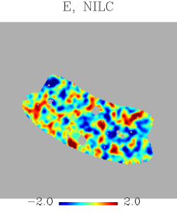
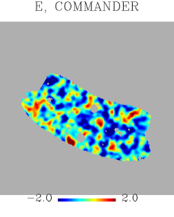
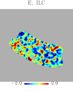
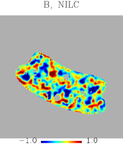
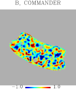
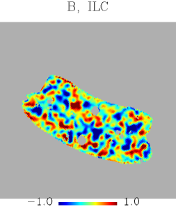
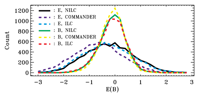
Figure 4: The E and B-components (top/middle) for the NILC, Commander and ILC maps. The bottom panel corresponds to the distribution function for the E and B components versus amplitude (mK).

The upper row of that figure represents the E-mode of polarisation, while the bottom row corresponds to the B-mode. Very preliminary visual inspection reveals obvious morphological similarity between NILC and ILC E-modes, and they strongly depart from the Commander map.

From figure 4 one can see that, compared to the ILC and NILC maps, the Commander E-map is strongly biased towards negative amplitudes. For the B-mode of all the maps the distribution functions are almost identical and Gaussian, with small fluctuations around $B=0\ \mu$K.

In order to understand the properties of the E/B-modes, we will use the same model as for the Q and U Stokes parameters for each Planck 2018 product:

$$E_{i}=E_{cmb}+E^{i}_{res}+E^{i}_{noise},$$

$$B_{i}=B_{cmb}+B^{i}_{res}+B^{i}_{noise}$$ (3.1)

where as previously, index $i$ labels the NILC, Commander and ILC maps, index $cmb$ stands for the frequency independent CMB component, index $res$ corresponds to the residuals of the foregrounds and systematics, and $noise$ stands for instrumental noise for each Planck 2018 map, including our ILC map. As we discussed in the previous section, the statistical properties of the E-mode are determined by the combination of the Gaussian components ($E_{cmb},E^{i}_{noise}$) and potentially the non-Gaussian tile $E_{res}$. For the B-mode, based on [20, 7, 21], we can safely neglect the CMB component, and focus on non-Gaussian residuals and Gaussian noise.

3.1 Analysis of the B-mode

If the foreground residuals plus systematics do not correlate with the instrumental noise it would be natural to assume that the shape of the corresponding distribution function of the B-mode will be represented by a Gaussian distribution with the standard deviation $\sigma_{B}$:

$$\sigma^{2}_{B}=\sigma^{2}_{noise}+\sigma^{2}_{res}$$ (3.2)

for all the B-mode products. Here $\sigma_{res}$ and $\sigma_{noise}$ denote the corresponding standard deviations for the residuals and instrumental noise. If $\sigma_{res}\ll\sigma_{noise}$, the distribution function in figure 4 should be similar to the PDF of the combined noise.

Input	E	B
NILC	0.95	0.46
Commander	0.97	0.51
ILC	0.99	0.53

Table 4: The standard deviation of the E- and B-modes in the BICEP2 region in $\mu$K.

Maps	Commander	100 GHz	143 GHz
NILC	0.95	0.16	0.63
Commander	—	0.30	0.69
100 GHz	—	—	0.08

Table 5: The cross correlation between the B-mode maps of different inputs in the BICEP2 region. Note that the standard deviation of the 100/143 GHz B-maps are 0.66/0.64 $\mu K^{2}$, respectively.

As it is seen from figure 4, for the B-mode the shape of distribution is very close to Gaussian distribution, with the standard deviations presented in table 4. These standard deviations differ between maps by about $10-20\%$, and the major sources of that difference are found in the signals with amplitudes $B<\sigma_{B}$, while for $B>\sigma_{B}$ the corresponding functions are remarkably similar. One can trace this similarity from figure 4 (middle panel), looking at the brightest positive and negative peaks. In order to understand the origin of that structure, one should look at the cross-correlation coefficients between some of the CMB products and the total B-mode signal at 100 and 143 GHz, presented in table 5. Firstly, NILC and Commander B-mode signals are correlated at 0.95 level. Secondly, the NILC B-mode consist at the level of 63% with 143 GHz signal and 16% with 100 GHz map. For the Commander map these coefficients are 69% and 30% correspondingly.

Strong correlations of the CMB products with the total frequency maps can be understood in terms of projection of the CMB products to the 100 and 143 GHz maps. For Commander, the amplitude of the B-mode can be presented as:

$$B_{c}=\alpha B_{100}+\beta B_{143}$$ (3.3)

where the coefficients $\alpha$ and $\beta$ are related to the cross-correlations coefficients $C^{c}_{100},C^{c}_{143}$ in table 5 as:

$$\alpha=\frac{1}{D}\left(dC^{c}_{100}-bC^{c}_{143}\right),\hskip 5.69046pt\beta=\frac{1}{D}\left(aC^{c}_{143}-cC^{c}_{100}\right)$$ (3.4)

and

$$D=ad-bc,\hskip 5.69046pta=\frac{\sigma_{100}}{\sigma_{c}},\hskip 5.69046ptb=C_{100,143}\frac{\sigma_{143}}{\sigma_{100}},\hskip 5.69046ptc=C_{100,143}\frac{\sigma_{100}}{\sigma_{c}},\hskip 5.69046ptd=\frac{\sigma_{143}}{\sigma_{c}}.$$ (3.5)

Here $C_{100,143}$ and $C^{c}_{100}$,$C^{c}_{143}$ are the cross-correlation coefficients between 100 and 143 GHz maps, and between Commander and 100,143 GHz maps correspondingly.

After simple algebra, from eqs. (3.4-3.5) and table 5 one can get: $\alpha\simeq 0.20$ and $\beta\simeq 0.53$. Thus, the Commander map consists of $\simeq 53\%$ of the signal from 143 GHz map, and $\simeq 20\%$ of the signal from 100 GHz map. The corresponding cross-correlations for Commander and NILC are very high for 143 GHz. They are almost 8 times greater then between 100 and 143 GHz.

3.2 Analysis of the E-mode

The E-mode of polarisation has a very important difference witn respect to the B-mode. In addition to the noise and residuals, the E-mode contains a significant primordial CMB component. This is why the distribution function for the E-mode in figure 4 has a standard deviation almost two times greater than the B-mode (see table 4). The common feature for all E-mode CMB products is a shift of the distribution to the negative amplitudes (mean values) by 0.3–0.7 $\mu K$, shown in figure 4.

In section 2.2 we have investigated the cross-correlations between the Stokes parameters Q and U for NILC and Commander and the corresponding residuals at 100 and 143 GHz. These cross-correlations are about $3.5\sigma$ to $5\sigma$ away from non-correlated Gaussian realisations. Here, in table 6, we present the correlations of the E-mode with the residuals, in order to see the effect of propagation of the Q/U anomalies to the E-mode.

Input	C	100 - N	100 - C	143 - N	143 - C
NILC (N)	$0.99$	$-0.25$	$-0.24$ $(3.8)$	$-0.21$	$-0.18$ $(2.8)$
Commander (C)	–	$-0.18$ $(2.8)$	$-0.19$	$-0.17$ $(2.7)$	$-0.17$
100 - N	–	–	$0.98$	$0.12$	$0.01$
100 - C	–	–	–	$0.07$	$0.00$
143 - N	–	–	–	–	$0.97$
143 - C	–	–	–	–	–

Table 6: The cross-correlation coefficients for NILC, Commander and the corresponding E-mode residuals maps at 100 and 143 GHz, and the significances (in brackets). Note that the significances can only be computed when at least one side is the CMB map.

4 Skewness and kurtosis for E and B modes

In the previous section we discussed the properties of the E- and B-modes in connection with their cross-correlations with the residuals at 100 and 143 GHz. Here we will investigate the third and forth moments of distribution functions of the E- and B-modes.

We have shown that due to non-locality of transition from Q/U components to E/B, the anomalies of the distribution function and skewness and kurtosis are significantly diluted. At the same time, the E-mode for the CMB maps is systematically shifted to the negative amplitudes, while the B-mode has a discrepancy at very low amplitudes. For the B-mode we have detected very significant cross-correlations between NILC and Commander maps with 143 GHz total map. Taking into account that for the Planck data we can safely neglect the primordial signal, these correlations can be related to absorption of the 143 GHz noise by the B-mode.

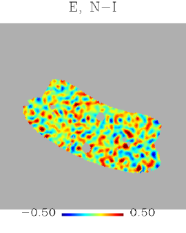
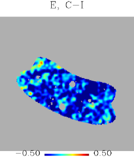
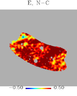
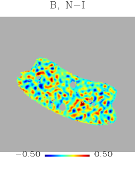
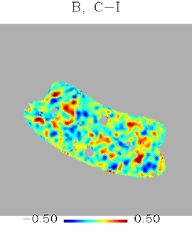
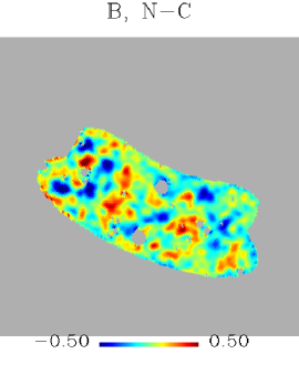
Figure 5: The maps of differences for E (upper row) and B (lower row) components for NILC–ILC (left), Commander–ILC (middle) and NILC–Commander (right panel).

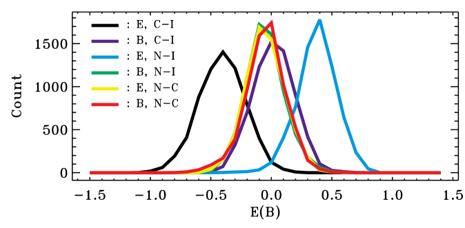
Figure 6: Histograms of the E- and B-maps of differences for Commander, NILC and ILC CMB products.

From figure 4 we have seen that the distribution function for the B-mode is close to Gaussian, while the E-mode is characterised by a relatively strong shift to negative mean values. However, it is not the only feature of the E-mode distribution. In table 7 we show the skewness and kurtosis of the E- and B-modes for the NILC, Commander and ILC polarisation maps, and of their differences, presented in figure 5 and figure 6.

Input	E-skewness	E-kurtosis	B-skewness	B-kurtosis
NILC	1.3	2.6	1.7	1.2
Commander	1.5	2.0	1.5	1.1
ILC	1.9	2.9	1.5	0.8
Commander–ILC	0.5	0.2	1.7	0.4
NILC–ILC	0.3	0.1	0.6	0.3
NILC–Commander	2.5	2.7	2.3	2.6

Table 7: The significance ($n\sigma$) of the skewness and kurtosis of E and B maps NILC, Commander, ILC maps and their differences. The numbers in the table correspond to the parameter $n$.

The E-modes for NILC, Commander and ILC are characterised by $2.0\sigma$ to $2.9\sigma$ departures from Gaussian realisations for the kurtosis. Note that the E- and B-mode for the difference NILC–Commander are peculiar at the level of $2.3\sigma$ to $2.7\sigma$ for the skewness and kurtosis. The comparison of the results, presented in table 7 and table 3 shows that the significance of the skewness and kurtosis under transition from Q/U to E/B is significantly reduced. This effect is quite understandable. This transition has non-local character as in multipole, as in pixel domain. Due to non-locality, the non-Gaussian features are redistributed among different pixels, reducing peculiarity of the E/B maps. Thus, one of the major conclusions following from our analysis is that tests on non-Gaussianity of E/B- map without Q/U components can easily produce misleading effects.

5 Conclusion

In our paper we have investigated the statistical properties of polarisation in the BICEP2 zone, basing our analysis on the Planck 2018 CMB products. One of the most interesting conclusions from our analysis is that Q and U Stokes parameters are more sensitive to the foreground residuals and possible systematics than the derived E/B-modes. We believe this effect is mainly due to non-locality of the $Q/U\rightarrow E/B$ transition, and removal of the E/B leakage. These tests have not been used previously in the analysis of statistical isotropy and non-Gaussianity of the Planck 2018 CMB products [22, 23] and allow us to evaluate the effectiveness of various methods for foreground component separation and validation of the polarization CMB signals.

We have shown that the NILC and Commander maps have very strong correlations with the residuals at 100 GHz with significance $3.5-5.2\sigma$, both for Q and U Stokes parameters.

After transition to the E/B modes, we have found a $2.6\sigma$ departure of the E-mode kurtosis statistic from Gaussianity for the NILC map, while the Commander map is characterised by a departure at the $2\sigma$ level. For these maps the B-mode skewness and kurtosis statistics lies within $1.5-1.7\sigma$. We have extended our analysis for the map of difference between NILC and Commander E/B-maps, in order to test the hypothesis that both these maps contain sub-dominant non-Gaussian residuals. We have found that E/B skewness and kurtosis for the difference map are peculiar at the level of $2.3-2.7\sigma$.

In conclusion, we would like to emphasize that the results obtained from the estimators adopted in this paper demonstrate that simple testing of statistical isotropy and non-Gaussian polarization of E and B modes is insufficient to confirm their cosmological nature for the new generation of CMB experiments. It is therefore important to complement these tests by analyzing the Q and U components, and especially their cross-correlations with the residual signals for a wide range of frequencies. When considering the potential Gaussian foregrounds far from the galactic plane, the analysis of these cross-correlations may be the most informative test.

References

- [1] M. Hazumi, J. Borrill, Y. Chinone, M. A. Dobbs, H. Fuke, A. Ghribi et al., LiteBIRD: a small satellite for the study of B-mode polarization and inflation from cosmic background radiation detection, in Space Telescopes and Instrumentation 2012: Optical, Infrared, and Millimeter Wave, vol. 8442 of Proc. SPIE, p. 844219, Sept., 2012, DOI.
- [2] K. N. Abazajian, P. Adshead, Z. Ahmed, S. W. Allen, D. Alonso, K. S. Arnold et al., CMB-S4 Science Book, First Edition, ArXiv e-prints (Oct., 2016) , [1610.02743].
- [3] B. Keating, S. Moyerman, D. Boettger, J. Edwards, G. Fuller, F. Matsuda et al., Ultra High Energy Cosmology with POLARBEAR, ArXiv e-prints (Oct., 2011) , [1110.2101].
- [4] J. A. Rubiño-Martín, R. Rebolo, M. Aguiar, R. Génova-Santos, F. Gómez-Reñasco, J. M. Herreros et al., The QUIJOTE-CMB experiment: studying the polarisation of the galactic and cosmological microwave emissions, .
- [5] H. Li, S.-Y. Li, Y. Liu, Y.-P. Li, Y. Cai, M. Li et al., Probing primordial gravitational waves: Ali CMB Polarization Telescope, National Science Review 6 (02, 2018) 145–154, [http://oup.prod.sis.lan/nsr/article-pdf/6/1/145/27981397/nwy019.pdf].
- [6] E. S. Battistelli, P. Ade, J. G. Alberro, A. Almela, G. Amico, L. H. Arnaldi et al., QUBIC: the Q & U Bolometric Interferometer for Cosmology, arXiv e-prints (Jan, 2020) arXiv:2001.10272, [2001.10272].
- [7] BICEP2 and Keck Array Collaborations, P. A. R. Ade, Z. Ahmed, R. W. Aikin, K. D. Alexander, D. Barkats et al., BICEP2/Keck Array V: Measurements of B-mode Polarization at Degree Angular Scales and 150 GHz by the Keck Array, Astrophys. J. 811 (Oct., 2015) 126, [1502.00643].
- [8] Planck collaboration, Y. Akrami et al., Planck 2018 results. IV. Diffuse component separation, 1807.06208.
- [9] K. Pearson, Note on Regression and Inheritance in the Case of Two Parents, Proceedings of the Royal Society of London Series I 58 (1895) 240–242.
- [10] M. Kamionkowski and E. D. Kovetz, Statistical diagnostics to identify galactic foregrounds in -mode maps, Phys. Rev. Lett. 113 (Nov, 2014) 191303.
- [11] H. Liu, S. von Hausegger and P. Naselsky, Towards understanding the Planck thermal dust models, Phys. Rev. D 95 (2017) 103517, [1705.05530].
- [12] S. von Hausegger, A. Gammelgaard Ravnebjerg and H. Liu, Statistical properties of polarized CMB foreground maps, Monthly Notices of the Royal Astronomical Society 487 (06, 2019) 5814–5823, [https://academic.oup.com/mnras/article-pdf/487/4/5814/28904721/stz1582.pdf].
- [13] Planck Collaboration, Y. Akrami, F. Arroja, M. Ashdown, J. Aumont, C. Baccigalupi et al., Planck 2018 results. I. Overview and the cosmological legacy of Planck, ArXiv e-prints (July, 2018) , [1807.06205].
- [14] H. K. Eriksen, A. J. Banday, K. M. Górski and P. B. Lilje, On Foreground Removal from the Wilkinson Microwave Anisotropy Probe Data by an Internal Linear Combination Method: Limitations and Implications, Astrophys. J. 612 (Sept., 2004) 633–646, [astro-ph/0403098].
- [15] M. Zaldarriaga and U. c. v. Seljak, All-sky analysis of polarization in the microwave background, Phys. Rev. D 55 (Feb, 1997) 1830–1840.
- [16] M. Kamionkowski, A. Kosowsky and A. Stebbins, Statistics of cosmic microwave background polarization, Phys. Rev. D 55 (June, 1997) 7368–7388, [astro-ph/9611125].
- [17] M. Zaldarriaga, Cosmic microwave background polarization experiments, The Astrophysical Journal 503 (1998) 1.
- [18] H. Liu, J. Creswell, S. von Hausegger and P. Naselsky, Methods for pixel domain correction of E B leakage, Phys. Rev. D 100 (Jul, 2019) 023538, [1811.04691].
- [19] H. Liu, General solutions of the leakage in integral transforms and applications to the EB-leakage and detection of the cosmological gravitational wave background, Journal of Cosmology and Astroparticle Physics 2019 (oct, 2019) 001–001.
- [20] BICEP2/Keck Collaboration, Planck Collaboration, P. A. R. Ade, N. Aghanim, Z. Ahmed, R. W. Aikin et al., Joint Analysis of BICEP2/Keck Array and Planck Data, Physical Review Letters 114 (Mar., 2015) 101301, [1502.00612].
- [21] Planck Collaboration, Y. Akrami, F. Arroja, M. Ashdown, J. Aumont, C. Baccigalupi et al., Planck 2018 results. X. Constraints on inflation, arXiv e-prints (July, 2018) arXiv:1807.06211, [1807.06211].
- [22] Planck Collaboration, P. A. R. Ade, N. Aghanim, Y. Akrami, P. K. Aluri, M. Arnaud et al., Planck 2015 results. XVI. Isotropy and statistics of the CMB, Astr. Astrophys. 594 (Sep, 2016) A16, [1506.07135].
- [23] Planck Collaboration, Y. Akrami, M. Ashdown, J. Aumont, C. Baccigalupi, M. Ballardini et al., Planck 2018 results. VII. Isotropy and Statistics of the CMB, arXiv e-prints (Jun, 2019) arXiv:1906.02552, [1906.02552].
- [24] K. M. Górski, E. Hivon, A. J. Banday, B. D. Wandelt, F. K. Hansen, M. Reinecke et al., HEALPix: A Framework for High-Resolution Discretization and Fast Analysis of Data Distributed on the Sphere, Astrophys. J. 622 (Apr., 2005) 759–771, [astro-ph/0409513].