A Separation Theorem for Joint Sensor and Actuator Scheduling
with Guaranteed Performance Bounds

Abstract

We study the problem of jointly designing a sparse sensor and actuator schedule for linear dynamical systems while guaranteeing a control/estimation performance that approximates the fully sensed/actuated setting. We further prove a separation principle, showing that the problem can be decomposed into finding sensor and actuator schedules separately. However, it is shown that this problem cannot be efficiently solved or approximated in polynomial, or even quasi-polynomial time for time-invariant sensor/actuator schedules; instead, we develop deterministic polynomial-time algorithms for a time-varying sensor/actuator schedule with guaranteed approximation bounds. Our main result is to provide a polynomial-time joint actuator and sensor schedule that on average selects only a constant number of sensors and actuators at each time step, irrespective of the dimension of the system. The key idea is to sparsify the controllability and observability Gramians while providing approximation guarantees for Hankel singular values. This idea is inspired by recent results in theoretical computer science literature on sparsification.

,

1 Introduction

One of the main challenges in realizing the promise of smart urban mobility is localization, perception, mapping and control with a myriad of sensors and actuators, e.g., camera sensors, data from 3-D mapping, LIDAR, electric motor, valve, etc. A key obstacle to this vision is the information overload, and the computational complexity of perception, mapping, and control using a large set of sensing and actuating modalities. A possible solution is to find a sparse yet important subset of sensors (actuators) and use those instead of using all available measurements (actuators) (Matni and Chandrasekaran, 2016; Argha et al., 2017; Fahroo and Demetriou, 2000). When the dimension of the state is large, finding the optimal yet low cardinality subset of features is like finding a needle in a haystack: the problem is computationally difficult and provably NP-Hard (Olshevsky, 2014; Tzoumas et al., 2016a).

Often times, we are interested in reducing the control complexity, operation cost, and maintenance cost by not using all available actuators and sensors. The choice of sensors and actuators affect the performance, computational cost, and costs of the control system. As it is shown recently in Olshevsky (2014) and Tzoumas et al. (2016a), the problem of finding a sparse set of input variables such that the resulting system is controllable, is NP-hard. Even the presumably easier problem of approximating the minimum number better than a constant multiplicative factor of $\log n$ is also NP-hard (Olshevsky, 2014). Other results in the literature have shown network controllability by exploring approximation algorithms for the closely related subset selection problem (Olshevsky, 2014; Summers et al., 2016; Pequito et al., 2015; Nozari et al., 2019; Bopardikar, 2017). More recently, some of the authors showed that even the problem of finding a sparse set of actuators to guarantee reachability of a particular state is hard and even hard to approximate (Jadbabaie et al., 2019).

Over the past few years, controllability and observability properties of complex dynamical networks have been subjects of intense study in the controls community (Olshevsky, 2014; Pasqualetti et al., 2014; Liu and Barabási, 2016; Chanekar et al., 2017; Müller and Weber, 1972; Tzoumas et al., 2016b; Olshevsky, 2015; Pequito et al., 2017; Nozari et al., 2017; Yazıcıoğlu et al., 2016; Summers et al., 2016; Pequito et al., 2015). This interest stems from the need to steer or observe the state of large-scale, networked systems such as power grids (Chakrabortty and Ilić, 2011), social networks, biological and genetic regulatory networks (Chandra et al., 2011; Marucci et al., 2009; Rajapakse et al., 2012), and traffic networks (Siami and Skaf, 2018). Previous studies have been mainly focused on solving the optimal sensor/actuator selection problem using the greedy heuristic, as approximations of the corresponding sparse-subset selection problem. However, in Jadbabaie et al. (2018a), we develop a framework to design a sparse actuator schedule for a given large-scale linear system with guaranteed performance bounds using deterministic polynomial-time and randomized approximately linear-time algorithms, and we gain new fundamental insights into approximating various performance metrics compared to the case when all actuators are chosen. In Tzoumas et al. (2018), the authors show that a separation principle holds for the Linear-Quadratic-Gaussian (LQG) control problem.

In this paper, we build upon our previous work (Jadbabaie et al., 2018a) and consider the problem of jointly designing the sparse sensor and actuator schedule for linear dynamical systems, to ensure desired performance and sparsity levels of active sensors and actuators in time and space. The joint sensor and actuator (S/A) scheduling problem involves selecting an appropriate number, activation time, position, and type of sensors and actuators. The idea is to essentially sparsify the choice of sensor and actuators both spatially and temporally. We show that by carefully designing a time-varying joint S/A selection strategy, one can choose, on average a constant number of sensors and actuators at each time, to approximate the Hankel singular values of the system, while sparsifying the sensor and actuator sets. One of our main contributions is to show that the classical time-varying joint S/A scheduling problem (originally studied by Athans (1972)), can be solved via random sampling. We also propose an alternative to submodularity-based methods and instead use recent advances in theoretical computer science.

More importantly, we prove that a separation principle holds for the problem of jointly sparsifying the sensor and actuator set with performance guarantees. We show that the joint S/A scheduling problem can be divided into two separate problems: the sparse sensor schedule and the sparse actuator schedule.

A preliminary version of some of our results in this article submitted for possible publication in a conference proceeding (Siami and Jadbabaie, 2019); however, their proofs are presented here for the first time. The manuscript also contains several new results including numerical examples, figures, tables, and proofs.

2 Preliminaries and Definitions

2.1 Mathematical Notations

Throughout the paper, discrete time index is denoted by $k$. The sets of real (integer), and non-negative real (integer) are represented by ${\mathbb{R}}$ ($\mathbb{Z}$), and ${\mathbb{R}}_{+}$ ($\mathbb{Z}_{+}$), respectively. The set of natural numbers $\{i\in{\mathbb{Z}}~{}:~{}1\leq i\leq n\}$ is denoted by $[n]$. The cardinality of a set $\sigma$ is denoted by $\operatorname{card}(\sigma)$. Capital letters, such as $A$ or $B$, stand for real-valued matrices. The $n$-by-$n$ identity matrix is denoted by $I$. Notation $A\preceq B$ is equivalent to matrix $B-A$ being positive semi-definite. The $n$ eigenvalues of $A\in{\mathbb{R}}^{n\times n}$ are shown by $\lambda_{1}(A),\lambda_{2}(A),\cdots,\lambda_{n}(A)$. $\lambda_{\max}(.)$ and $\sigma_{\max}(.)$ show the largest eigenvalue and singularvalue of a matrix, respectively. The transpose of matrix $A$ is denoted by $A^{\top}$. The rank of matrix $A$ is referred to by $\operatorname{rank}(A)$.

2.2 Linear Systems, Gramian and Hankel Matrices

We start with the canonical linear discrete-time, time-invariant dynamics

$$x(k+1)~{}=~{}A\,x(k)~{}+~{}B\,u(k),$$ (1)

$$y(k)~{}=~{}Cx(k),$$ (2)

where $A\in{\mathbb{R}}^{n\times n}$, $B\in{\mathbb{R}}^{n\times m}$, $C\in{\mathbb{R}}^{p\times n}$ and $k\in{\mathbb{Z}}_{+}$. The state matrix $A$ describes the underlying structure of the system and the interaction strength between the agents, input matrix $B$ represents how the control input enters the system, and output matrix $C$ shows how output vector $y$ relates to the state vector.

The controllability and observability matrices at time $t$ (where $t\geq n$) are given by

$$\mathcal{R}(t)~{}=~{}\left[B~{}AB~{}A^{2}B~{}\cdots~{}A^{t-1}B\right],$$ (3)

and

$$\mathcal{O}(t)~{}=~{}\begin{bmatrix}C\\ CA\\ CA^{2}\\ \cdots\\ CA^{t-1}\end{bmatrix},$$ (4)

respectively. It is well-known that from a numerical standpoint it is better to characterize controllability and observability in terms of the Gramian matrices at time $t$ defined as follows:

$$\mathcal{P}(t)~{}=~{}\sum_{i=0}^{t-1}A^{i}BB^{\top}(A^{i})^{\top}~{}=~{}\mathcal{R}(t)\,\mathcal{R}^{\top}(t),$$ (5)

and

$$\mathcal{Q}(t)~{}=~{}\sum_{i=0}^{t-1}(A^{i})^{\top}C^{\top}CA^{i}~{}=~{}\mathcal{O}^{\top}(t)\,\mathcal{O}(t).$$ (6)

Assumption 1.

Throughout the paper, we assume that the system (1)-(2) is an $n$-state minimal realization (i.e., the reachability and controllability matrices have full row rank). However, all results presented in this paper can be modified/extended to uncontrollable and unobservable systems.

For given linear systems (1)-(2), the Hankel matrix is defined as the doubly infinite matrix

$$\tiny\mathcal{H} = \begin{bmatrix}H_{1}&H_{2}&H_{3}&\cdots\\ H_{2}&H_{3}&H_{4}&\cdots\\ H_{3}&H_{4}&H_{5}&\cdots\\ \vdots&\vdots&\vdots&\ddots\end{bmatrix}$$

$$= \begin{bmatrix}C\\ CA\\ CA^{2}\\ \vdots\end{bmatrix}\begin{bmatrix}B&AB&A^{2}B&\cdots~{}\end{bmatrix}$$

$$= \mathcal{O}\mathcal{R},$$

where $H_{k}=CA^{k-1}B$. The Hankel matrix can be viewed as a mapping between the past inputs and future outputs via the initial state $x(0)$. Since $\mathcal{H}=\mathcal{O}\mathcal{R}$ and due to Assumption 1, it follows that $\text{rank}(\mathcal{H})=n$. The $n$ nonzero singular values of $\mathcal{H}$ can be computed by solving two Lyapunov equations (for controllability and observability Gramians) as follows

$$\sigma_{i}(\mathcal{H}) = \sqrt{\lambda_{i}(\mathcal{H}\mathcal{H}^{\top})}$$

$$= \sigma_{i}(\mathcal{P}\mathcal{Q})$$

$$= \lambda_{i}(\mathcal{Q}^{\frac{1}{2}}\mathcal{P}\mathcal{Q}^{\frac{1}{2}}).$$

The Hankel matrix has a special structure: the elements (blocks) in lines parallel to the anti-diagonal are identical. It is well-known that the singular values of the Hankel matrix of a linear system are fundamental invariants of the system, denoting the most controllable and observable modes (Antoulas, 2005). It is well known that the states corresponding to small nonzero Hankel singular values are difficult to control and observe at the same time.

The Hankel norm gives the $L_{2}$-gain from past inputs to future outputs, and measures the extent to which past inputs effect future outputs of the system. If the input $u(k)=0$ for $k\geq 0$ and the output is $y(k)$, then the Hankel norm is given by

$$\|G(z)\|_{H} := \sup_{u\in\mathcal{L}_{2}(-\infty,0)}\frac{\sum_{t=1}^{\infty}|y(t)|^{2}}{\sum_{t=1}^{\infty}|u(-t)|^{2}}$$

$$= \sqrt{\lambda_{\max}(\mathcal{P}\mathcal{Q})}~{}=~{}\sigma_{\max}(\mathcal{H}),$$

where $G(z)$ is a transfer function of dynamics (1)-(2), and $\mathcal{L}_{2}(-\infty,0)$ is the space of square summable vector sequences in the interval $(-\infty,0)$ (which means $\sum_{t=1}^{\infty}|u(-t)|^{2}\leq\infty$). In this work, we focus on the time-$t$ Hankel matrix

$$\tiny\mathcal{H}(t) = \begin{bmatrix}H_{1}&H_{2}&H_{3}&\cdots&H_{t}\\ H_{2}&H_{3}&H_{4}&\cdots&H_{t+1}\\ H_{3}&H_{4}&H_{5}&\cdots&H_{t+2}\\ &&\cdots&&\\ H_{t}&H_{t+1}&H_{t+2}&\cdots&H_{2t-1}\end{bmatrix}$$

$$= \begin{bmatrix}C\\ CA\\ CA^{2}\\ \cdots\\ CA^{t-1}\end{bmatrix}\begin{bmatrix}B&AB&A^{2}B&\cdots&A^{t-1}B\end{bmatrix}$$

$$= \mathcal{O}(t)\mathcal{R}(t).$$

Particularly, we have

$$\sigma_{i}(\mathcal{H}(t)) = \sqrt{\lambda_{i}(\mathcal{H}(t)\mathcal{H}^{\top}(t))}=\sigma_{i}(\mathcal{P}(t)\mathcal{Q}(t))$$

$$= \lambda_{i}(\mathcal{Q}^{\frac{1}{2}}(t)\mathcal{P}(t)\mathcal{Q}^{\frac{1}{2}}(t)).$$

Remark 1.

One way to lower the computational complexity of simulations of large-scale dynamical systems is finding a reduced-order model. A common technique for model order reduction is the optimal Hankel-norm approximation. This method provides the best approximation of the original system in the Hankel semi-norm and received significant attention and related development in the 1980s (Glover, 1987). The corresponding state-space realization is the balanced realization where $\tilde{\mathcal{P}}=\tilde{\mathcal{Q}}=\operatorname{diag}(\sigma_{1},\cdots,\sigma_{n})$ as proposed Moore (1981). In standard model reduction, first we obtain the balanced realization, and then the least observable and controllable modes are truncated. However, for sparse S/A schedule, we sparsify inputs and outputs in space and time (the number of states does not change) and we utilize a different canonical state realization (see Section 5).

2.3 Hankel-based Performance Metrics

Similar to the systemic notions introduced in Siami and Motee (2018); Jadbabaie et al. (2018a), we define various performance metrics that capture both controllability and observability properties of the system. These measures are non-negative real-valued operators defined on the set of all linear dynamical systems governed by (1)-(2) and quantify various measures of the performance. All of the metrics depend on the symmetric combination of Gramians (i.e. $\mathcal{Q}^{\frac{1}{2}}(t)\mathcal{P}(t)\mathcal{Q}^{\frac{1}{2}}(t)$) which is a positive definite matrix. Therefore, one can define a systemic Hankel-based performance measure as an operator on the set of Gramian matrices of all $n$-state minimal realization systems, which we represent by $\mathbb{S}_{+}^{n}$. We denote the Hankel-based Performance Metrics by $\rho:\mathbb{S}_{+}^{n}\rightarrow\mathbb{R}$. For many popular choices of $\rho$, one can see that they satisfy the following properties

(i) Homogeneity: for all $\kappa>1$,

$${\rho}(\kappa A)~{}=~{}\kappa{\rho}(A);$$

(ii) Monotonicity: if $A\preceq B$, then

$${\rho}(A)~{}\leq~{}{\rho}(B);$$

and we call them systemic. For example, the squared Hankel-norm of the system at time $t$ which is defined by

$$\rho(\mathcal{Q}^{\frac{1}{2}}(t)\mathcal{P}(t)\mathcal{Q}^{\frac{1}{2}}(t)):=\lambda_{\max}(\mathcal{Q}^{\frac{1}{2}}(t)\mathcal{P}(t)\mathcal{Q}^{\frac{1}{2}}(t)),$$

is systemic. We note that similar criteria have been developed in the experiment design literature (Ravi et al., 2016; Kempthorne, 1952; Allen-Zhu et al., 2017).

3 Matrix Reconstruction and Sparsification

The key idea in Jadbabaie et al. (2018b) and Jadbabaie et al. (2018a) is to approximate the time-$t$ controllability Gramian as a sparse sum of rank-$1$ matrices, while controlling the approximation error. To this end, a key lemma is used in Jadbabaie et al. (2018a) from the sparsification literature (Boutsidis et al., 2014) to find sparse actuator or sensor schedules. However, in the present work, we are interested in designing a joint sparse schedule for both sensor and actuator sets; for this, we need to modify a key lemma, known as the Dual Set Lemma in Boutsidis et al. (2014) to approximate the time-$t$ Hankel singular values.

Our main result in this section shows how we can handle two sparse subsets with nonidentical indices. We then use this result later to design a deterministic algorithm for a joint sparse S/A schedule. More specifically, we need to control the singular values of the product of two matrices which can be written as the symmetrized combination of the two matrices (see Section 5). Each one of these matrices is a sparse sum of rank-$1$ matrices and they reflect controllability and observability properties of the chosen sparse S/A set.

Theorem 1 and Algorithm 1 formalize the procedure of iteratively adding one vector at a time and forming two Gramian matrices.

Theorem 1.

Let $V=\{v_{1},\ldots,v_{t_{1}}\}$ and $U=\{u_{1},\ldots,u_{t_{2}}\}$ such that $\sum_{i=1}^{t_{1}}v_{i}v_{i}^{\top}=X$ and $\sum_{i=1}^{t_{2}}u_{i}u_{i}^{\top}=I_{n}$ where $v_{i},u_{i}\in{\mathbb{R}}^{n}$ ($n<t_{1},t_{2}$). Given integer numbers $\kappa_{1}$ and $\kappa_{2}$ with $n<\kappa_{1}\leq t_{1}$ and $n<\kappa_{2}\leq t_{2}$, Algorithm 1 computes a set of weights $s_{i}\geq 0$ and $r_{i}\geq 0$, such that

$$\left(\sum_{i=1}^{t_{1}}s_{i}v_{i}v_{i}^{\top}\right)^{\frac{1}{2}}\left(\sum_{i=1}^{t_{2}}r_{i}u_{i}u_{i}^{\top}\right)\left(\sum_{i=1}^{t_{1}}s_{i}v_{i}v_{i}^{\top}\right)^{\frac{1}{2}}$$

$$~{}~{}~{}~{}~{}~{}~{}~{}~{}~{}~{}~{}~{}~{}\succeq~{}{\rm e}^{-(\epsilon_{1}+\epsilon_{2})}X,$$

$$\left(\sum_{i=1}^{t_{1}}s_{i}v_{i}v_{i}^{\top}\right)^{\frac{1}{2}}\left(\sum_{i=1}^{t_{2}}r_{i}u_{i}u_{i}^{\top}\right)\left(\sum_{i=1}^{t_{1}}s_{i}v_{i}v_{i}^{\top}\right)^{\frac{1}{2}}$$

$$~{}~{}~{}~{}~{}~{}~{}~{}~{}~{}~{}~{}~{}~{}\preceq~{}{\rm e}^{\epsilon_{1}+\epsilon_{2}}X,$$

$$\operatorname{card}\left\{s_{i}\neq 0~{}|~{}i\in[t_{1}]\right\}~{}\leq~{}\kappa_{1},$$

and

$$\operatorname{card}\left\{r_{i}\neq 0~{}|~{}i\in[t_{2}]\right\}~{}\leq~{}\kappa_{2},$$

where

$$\epsilon_{1}~{}:=~{}2\tanh^{-1}\left(\sqrt{\frac{n}{\kappa_{1}}}\right),~{}\text{and}~{}\epsilon_{2}~{}:=~{}2\tanh^{-1}\left(\sqrt{\frac{n}{\kappa_{2}}}\right).$$

Due to space limitations, we refer the interested readers to (Boutsidis et al., 2014) for more details on Algorithm 1. However, roughly speaking, the algorithm is based on choosing vectors in a greedy fashion that satisfy a set of desired properties at each step, leading to bounds on Hankel singular values. We first define two barriers or potential functions as follows:

$$\underline{\phi}(\underline{\mu},\underline{\mathcal{A}})=\sum_{i=1}^{n}\frac{1}{\lambda_{i}(\underline{\mathcal{A}})-\underline{\mu}},$$ (7)

and

$$\bar{\phi}(\bar{\mu},\bar{\mathcal{A}})~{}=~{}\sum_{i=1}^{n}\frac{1}{\bar{\mu}-\lambda_{i}(\bar{\mathcal{A}})}.$$ (8)

These potential functions quantify how far the eigenvalues of $\underline{\mathcal{A}}$ and $\bar{\mathcal{A}}$ are from the barriers $\underline{\mu}$ and $\bar{\mu}$. These potential functions blow up as any eigenvalue nears the barriers; moreover, they show the locations of all the eigenvalues concurrently. We then define two parameters $\mathfrak{L}$ and $\mathfrak{U}$ as follows:

$$\mathfrak{L}(v,\underline{\delta},\underline{\mathcal{A}},\underline{\mu})~{}=$$

$$~{}~{}\frac{v^{\top}\left(\underline{\mathcal{A}}-(\underline{\mu}+\underline{\delta})I_{n}\right)^{-2}v}{\underline{\phi}(\underline{\mu}+\underline{\delta},\underline{\mathcal{A}})-\underline{\phi}(\underline{\mu},\underline{\mathcal{A}})}-v^{\top}\left(\underline{\mathcal{A}}-(\underline{\mu}+\underline{\delta})I_{n}\right)^{-1}v,$$

and

$$\mathfrak{U}(u,\bar{\delta},\bar{\mathcal{A}},\bar{\mu})=$$

$$~{}~{}\frac{u^{\top}((\bar{\mu}+\bar{\delta})I_{n}-\bar{\mathcal{A}})^{-2}u}{\bar{\phi}(\bar{\mu},\bar{\mathcal{A}})-\bar{\phi}(\bar{\mu}+\bar{\delta},\bar{\mathcal{A}})}+u^{\top}\left((\bar{\mu}+\bar{\delta})I_{n}-\bar{\mathcal{A}}\right)^{-1}u.$$

The Sherman-Morrison-Woodbury formula inspires the structure of the above quantities for more details on the barrier method see (Boutsidis et al., 2014). The potential functions (7) and (8) are chosen to guide the selection of vectors and scalings at each step $\tau$ and to ensure steady progress of the algorithm. Small values of these potentials indicate that the eigenvalues of $\bar{\mathcal{A}}$ and $\underline{\mathcal{A}}$ do not gather near $\bar{\mu}$ and $\underline{\mu}$, respectively. At each iteration, we increase the upper barrier $\bar{\mu}$ by a fixed constant $\bar{\delta}$ and the lower barrier $\bar{\mu}$ by another fixed constant $\underline{\delta}$. It can be shown that as long as the potentials remain bounded, there must exist (at every step $\tau$) a choice of an index $j$ and weights $s_{j}$ and $r_{j}$ so that the addition of the associated rank-1 matrices to $\bar{\mathcal{A}}$ and $\underline{\mathcal{A}}$, and the increments of barriers do not increase either potential and keep all the eigenvalues of the updated matrix between the barriers (see Algorithm 1). Repeating these steps ensures steady growth of all the eigenvalues and yields the desired result.

This algorithm is tailored from an algorithm from Boutsidis et al. (2014) (which is deterministic and requires at most $\mathcal{O}\left((\kappa_{1}t_{1}+\kappa_{2}t_{2})n^{2}\right)$) steps for joint sparse S/A selections. We view this algorithm as a subroutine acting on sets $U$ and $V$ as

$$s,r=\operatorname{GenDualSet}(V,U,\kappa_{1},\kappa_{2}).$$

Algorithm 1 A Modified Dual Set Spectral Sparsification $\operatorname{GenDualSet}(V,U,\kappa_{1},\kappa_{2})$.

1:Input $V=\left[v_{1},\ldots,v_{t_{1}}\right]\in{\mathbb{R}}^{n\times t_{1}}$, with $VV^{\top}=X$, $U=\left[u_{1},\ldots,u_{t_{2}}\right]\in{\mathbb{R}}^{n\times t_{2}}$, with $UU^{\top}=I_{n}$, $\kappa_{1}\in{\mathbb{Z}}_{+}$, with $n<\kappa_{1}\leq t_{1}$, $\kappa_{2}\in{\mathbb{Z}}_{+}$, with $n<\kappa_{2}\leq t_{2}$

2:Output $s=[s_{1},s_{2},\ldots,s_{t_{1}}]\in{\mathbb{R}}^{1\times t_{1}}_{+}$ with $\|s\|_{0}\leq\kappa_{1}$, $r=[r_{1},r_{2},\ldots,r_{t_{2}}]\in{\mathbb{R}}^{1\times t_{2}}_{+}$ with $\|r\|_{0}\leq\kappa_{2}$,

3:Set $s(0)=0_{t_{1}\times 1}$, $\underline{\mathcal{A}}(0)=\bar{\mathcal{A}}(0)=0_{n\times n}$, $\underline{\delta}=1$, $\bar{\delta}=\frac{1+\sqrt{\frac{n}{\kappa_{1}}}}{1-\sqrt{\frac{n}{\kappa_{1}}}}$

4:for $\tau=0:\kappa_{1}-1$ do

5:     $\underline{\mu}({\tau})=\tau-\sqrt{\kappa_{1}n}$

6:     $\bar{\mu}({\tau})=\bar{\delta}\left(\tau+\sqrt{\kappa_{1}n}\right)$

7:     Find an index $j$ such that

$$\mathfrak{U}(X^{-\frac{1}{2}}v_{j},\bar{\delta},\bar{\mathcal{A}}(\tau),\bar{\mu}({\tau}))\leq\mathfrak{L}(X^{-\frac{1}{2}}v_{j},\underline{\delta},\underline{\mathcal{A}}({\tau}),\underline{\mu}({\tau}))$$

8:     Set

9:     Update the $j$-th component of $s(\tau)$: $s({\tau+1})=s(\tau)+\Delta\text{e}_{j}$,

10:     $\underline{\mathcal{A}}({\tau+1})=\underline{\mathcal{A}}({\tau})+\Delta X^{-\frac{1}{2}}v_{j}v_{j}^{\top}X^{-\frac{1}{2}}$

11:     $\bar{\mathcal{A}}({\tau+1})=\bar{\mathcal{A}}({\tau})+\Delta X^{-\frac{1}{2}}u_{j}u_{j}^{\top}X^{-\frac{1}{2}}$

12:end for

13:Set $r(0)=0_{t_{2}\times 1}$, $\underline{\mathcal{A}}(0)=\bar{\mathcal{A}}(0)=0_{n\times n}$, $\underline{\delta}=1$, $\bar{\delta}=\frac{1+\sqrt{\frac{n}{\kappa_{2}}}}{1-\sqrt{\frac{n}{\kappa_{2}}}}$

14:for $\tau=0:\kappa_{2}-1$ do

15:     $\underline{\mu}({\tau})=\tau-\sqrt{\kappa_{2}n}$

16:     $\bar{\mu}({\tau})=\bar{\delta}\left(\tau+\sqrt{\kappa_{2}n}\right)$

17:     Find an index $j$ such that

$$\mathfrak{U}(u_{j},\bar{\delta},\bar{\mathcal{A}}(\tau),\bar{\mu}({\tau}))\leq\mathfrak{L}(u_{j},\underline{\delta},\underline{\mathcal{A}}({\tau}),\underline{\mu}({\tau}))$$

18:     Set

$$\Delta={2}{\left(\mathfrak{U}(u_{j},\bar{\delta},\bar{\mathcal{A}}(\tau),\bar{\mu}({\tau}))+\mathfrak{L}(u_{j},\underline{\delta},\underline{\mathcal{A}}({\tau}),\underline{\mu}({\tau}))\right)^{-1}}$$

19:     Update the $j$-th component of $r(\tau)$:

$$r({\tau+1})=r(\tau)+\Delta\text{e}_{j},$$

20:     $\underline{\mathcal{A}}({\tau+1})=\underline{\mathcal{A}}({\tau})+\Delta u_{j}u_{j}^{\top}$

21:     $\bar{\mathcal{A}}({\tau+1})=\bar{\mathcal{A}}({\tau})+\Delta u_{j}u_{j}^{\top}$

22:end for

23:Return

$$s=\kappa_{1}^{-1}\left(1-\sqrt{\frac{n}{\kappa_{1}}}\right)s(\kappa_{1})$$

$$r=\kappa_{2}^{-1}\left(1-\sqrt{\frac{n}{\kappa_{2}}}\right)r(\kappa_{2})$$

We now present the proof of Theorem 1.

Proof 1.

To prove this theorem we first use (Boutsidis et al., 2014, Lemma 1). We first define an isotropic set of $t_{1}$ vectors based on set $V=\{v_{1},\ldots,v_{t_{1}}\}$ as follows

$$\bar{V}=\{\bar{v}_{i}=X^{-\frac{1}{2}}v_{i}|~{}v_{i}\in V\}.$$ (9)

Using (9), we have

$$\sum_{i=1}^{t_{1}}\bar{v}_{i}\bar{v}_{i}^{\top}=I_{n}.$$ (10)

Then, according to the Dual Set Lemma in Boutsidis et al. (2014) and Line 1 to Line 10 of Algorithm 1 where $\bar{s}=\kappa_{1}^{-1}\left(1-\sqrt{\frac{n}{\kappa_{1}}}\right)s(\kappa_{1})$, we get

$$\left(1-\sqrt{\frac{n}{\kappa_{1}}}\right)^{2}I_{n}~{}\preceq~{}\sum_{i=1}^{t_{1}}\bar{s}_{i}\bar{v}_{i}\bar{v}_{i}^{\top}~{}\preceq~{}\left(1+\sqrt{\frac{n}{\kappa_{1}}}\right)^{2}I_{n},$$ (11)

where $\operatorname{card}\{s_{i}\neq 0|~{}i\in[t_{1}]\}\leq\kappa_{1}$. This can be rewritten as follows

$${\rm e}^{-\epsilon_{1}}I_{n}~{}\preceq~{}\sum_{i=1}^{t_{1}}s_{i}\bar{v}_{i}\bar{v}_{i}^{\top}~{}\preceq~{}{\rm e}^{-\epsilon_{1}}I_{n},$$ (12)

where $\epsilon_{1}=2\tanh^{-1}\left(\sqrt{\frac{n}{\kappa_{1}}}\right)$, and

$$s=\kappa_{1}^{-1}\left(1+\sqrt{\frac{n}{\kappa_{1}}}\right)^{-1}s(\kappa_{1}),$$

where $s(.)$ is defined in Algorithm 1 and $s=[s_{1},s_{2},\cdots,s_{t_{1}}]$. Next, based on (10), (11), and $\sum_{i=1}^{t_{1}}v_{i}v_{i}^{\top}=X$, we get

$${\rm e}^{-\epsilon_{1}}X~{}\preceq~{}\sum_{i=1}^{t_{1}}s_{i}v_{i}v_{i}^{\top}~{}\preceq~{}{\rm e}^{\epsilon_{1}}X,$$ (13)

where (13) is obtained by multiplying positive definite matrix $X^{\frac{1}{2}}$ from both sides of (11). Similarly, according to the Dual Set Lemma in Boutsidis et al. (2014) and Line 11 to Line 21 of Algorithm 1 where $\bar{r}=\kappa_{2}^{-1}\left(1-\sqrt{\frac{n}{\kappa_{2}}}\right)r(\kappa_{2})$, we get

$$\left(1-\sqrt{\frac{n}{\kappa_{2}}}\right)^{2}I_{n}~{}\preceq~{}\sum_{i=1}^{t_{2}}\bar{r}_{i}u_{i}u_{i}^{\top}~{}\preceq~{}\left(1+\sqrt{\frac{n}{\kappa_{2}}}\right)^{2}I_{n},$$ (14)

where $\operatorname{card}\{r_{i}\neq 0|~{}i\in[t_{2}]\}\leq\kappa_{2}$. This can be rewritten as follows

$${\rm e}^{-\epsilon_{2}}I_{n}~{}\preceq~{}\sum_{i=1}^{t_{2}}r_{i}u_{i}u_{i}^{\top}~{}\preceq~{}{\rm e}^{-\epsilon_{2}}I_{n},$$ (15)

where $\epsilon_{2}=2\tanh^{-1}\left(\sqrt{\frac{n}{\kappa_{2}}}\right)$, and

$$r=\kappa_{2}^{-1}\left(1+\sqrt{\frac{n}{\kappa_{2}}}\right)^{-1}r(\kappa_{2}),$$

where $r(.)$ is defined in Algorithm 1 and $r=[r_{1},r_{2},\cdots,r_{t_{2}}]$. Using (14) and the fact that $\left(\sum_{i=1}^{t_{1}}s_{i}v_{i}v_{i}^{\top}\right)^{\frac{1}{2}}\succeq 0$, it follows

$${\rm e}^{-\epsilon_{2}}\sum_{i=1}^{t_{1}}s_{i}v_{i}v_{i}^{\top}~{}\preceq~{}~{}~{}~{}~{}~{}~{}~{}~{}~{}~{}~{}~{}~{}~{}~{}~{}~{}~{}~{}~{}~{}~{}~{}~{}~{}~{}~{}~{}~{}~{}$$

$$\left(\sum_{i=1}^{t_{1}}s_{i}v_{i}v_{i}^{\top}\right)^{\frac{1}{2}}\left(\sum_{i=1}^{t_{2}}r_{i}u_{i}u_{i}^{\top}\right)\left(\sum_{i=1}^{t_{1}}s_{i}v_{i}v_{i}^{\top}\right)^{\frac{1}{2}}$$

$$\preceq~{}{\rm e}^{\epsilon_{2}}\sum_{i=1}^{t_{1}}s_{i}v_{i}v_{i}^{\top}.$$ (16)

Finally combining (13) and (16), we get the desired results.

In the next section, we show how various Hankel-based measures can be approximated by selecting a sparse set of actuators and sensors.

4 Joint Sparse S/A Scheduling Problems

For given linear system (1)-(2) with a general underlying structure, the joint S/A scheduling problem seeks to construct a schedule of the control inputs and sensor outputs that keeps the number of active actuators and sensors much less than the fully sensed/actuated system such that the Hankel-based performance matrices of the original and the new systems are similar in an appropriately defined sense. Specifically, given a canonical linear, time-invariant system (1)-(2) with $m$ actuators, $p$ sensors and Gramians $\mathcal{P}(t)$, $\mathcal{Q}(t)$ at time $t$, our goal is to find a joint sparse S/A schedule such that the resulting system with Hankel matrix $\mathcal{H}_{s}(t)$ is well-approximated, i.e.,

$$\left|\log\frac{\rho\left(\mathcal{Q}^{\frac{1}{2}}(t)\mathcal{P}(t)\mathcal{Q}^{\frac{1}{2}}(t)\right)}{\rho\left(\mathcal{Q}_{s}^{\frac{1}{2}}(t)\mathcal{P}_{s}(t)\mathcal{Q}_{s}^{\frac{1}{2}}(t)\right)}\right|~{}\leq~{}\epsilon,$$ (17)

where $\rho$ is any systemic performance metric that quantifies the performance of the system for example as the $\mathcal{L}_{2}$-gain from past inputs to future outputs, and $\epsilon\geq 0$ is the approximation factor. The systemic performance metrics are defined based on the Hankel singular values, and we will show that “close” controllability and observability Gramian matrices result in approximately the same values. Our goal here is to answer the following questions: (1) What are the minimum numbers of actuators and sensors that need to be chosen to achieve a good approximation of the system where the full sets of actuators and sensors utilized? (2) What is the relation between the numbers of selected actuators and sensors and performance loss? (3) Does a sparse approximation schedule exist with at most constant numbers of active actuators and sensors at each time? (4) What is the time complexity of choosing the subsets of actuators and sensors with guaranteed performance bounds?

In the rest of this paper, we show how some fairly recent advances in theoretical computer science can be utilized to answer these questions. Recently, Marcus, Spielman, and Srivastava introduced a new variant of the probabilistic method which ends up solving the so-called Kadison-Singer (KS) conjecture (Marcus et al., 2015). We use the solution approach to the KS conjecture together with a combination of tools from Sections 4 and 5 to find a sparse approximation of the sparse S/A scheduling problem with algorithms that have favorable time-complexity.

5 A Weighted Joint Sparse S/A Schedule

As a starting point, we allow for scaling of the selected input and output signals while keeping the input and output scaling bounded. The input and output scalings allow for an extra degree of freedom that could allow for further sparsification of the sensor/actuator set. Given (1)-(2), we define a weighted, joint sensor and actuator schedule by

$$\sigma~{}=~{}\left(\{\sigma^{\text{(s)}}_{k}\}_{k=0}^{t-1},\{\sigma^{\text{(a)}}_{k}\}_{k=0}^{t-1}\right),$$

where

$$\sigma^{\text{(s)}}_{k}=\left\{i|\,\mathfrak{s}_{i}(k)>0,~{}i\in[p]\right\}\subseteq[p],$$

$$\sigma^{\text{(a)}}_{k}=\left\{i|\,\mathfrak{a}_{i}(k)>0,~{}i\in[m]\right\}\subseteq[m],$$

and non-negative input and output scalings (i.e., $\mathfrak{a}_{i}(k)\geq 0$, $\mathfrak{s}_{i}(k)\geq 0$). The resulting system with this schedule is

$$x(k+1) = A\,x(k)\,+\,\sum_{i\in\sigma^{\text{(a)}}_{k}}\mathfrak{a}_{i}(k)\,b_{i}\,u_{i}(k),$$ (18)

$$y(k) = \sum_{i\in\sigma^{\text{(s)}}_{k}}\mathfrak{s}_{i}(k)\,{\text{e}}_{i}\,c_{i}\,x(k),$$ (19)

where $b_{i}$’s are columns of matrix $B\in{\mathbb{R}}^{n\times m}$, $c_{i}$’s are rows of matrix $C\in{\mathbb{R}}^{p\times n}$, and $\text{e}_{i}$’s are the standard basis for ${\mathbb{R}}^{p}$; scaling $\mathfrak{a}_{i}(k)\geq 0$ shows the strength of the $i$-th control input at time $k$; and similarly $\mathfrak{s}_{i}(k)\geq 0$ shows the strength of the $i$-th output at time $k$. Equivalently, the dynamics can be rewritten as

$$x(k+1)~{}=~{}A\,x(k)~{}+~{}\mathcal{B}(k)\,u(k),$$ (20)

$$y(k)~{}=~{}\mathcal{C}(k)\,x(k),$$ (21)

with time-varying input and output matrices

$$\mathcal{B}(k)~{}=~{}B\,\Lambda(k),$$

and

$$\mathcal{C}(k)~{}=~{}\Gamma(k)\,C,$$

where $\Lambda(k)$ and $\Gamma(k)$ are diagonal, and their nonzero diagonal entries show selected actuators and sensors at time $k$, which means

$$\Lambda(k)=\operatorname{diag}\left(\mathfrak{a}_{1}(k),\cdots,\mathfrak{a}_{m}(k)\right),$$

and

$$\Gamma(k)=\operatorname{diag}\left(\mathfrak{s}_{1}(k),\cdots,\mathfrak{s}_{p}(k)\right).$$

The controllability Gramian and observability Gramian at time $t$ for this system can be rewritten as

$$\mathcal{P}_{s}(t)~{}=~{}\sum_{k=0}^{t-1}\sum_{j\in\sigma^{\text{(a)}}_{k}}\mathfrak{a}_{j}^{2}(k)\left(A^{t-k-1}b_{j}\right)\left(A^{t-k-1}b_{j}\right)^{\top},$$ (22)

and

$$\mathcal{Q}_{s}(t)~{}=~{}\sum_{k=0}^{t-1}\sum_{j\in\sigma^{\text{(s)}}_{k}}\mathfrak{s}_{j}^{2}(k)\left(c_{j}A^{t-k-1}\right)^{\top}\left(c_{j}A^{t-k-1}\right).$$ (23)

Our goal is to keep the numbers of active sensors and actuators on average less than $d_{\text{s}}$ and $d_{\text{a}}$, i.e.,

$$\frac{\sum_{k=0}^{t-1}\operatorname{card}\left\{\sigma^{\text{(s)}}_{k}\right\}}{t}~{}\leq~{}d_{\text{s}},$$ (24)

and

$$\frac{\sum_{k=0}^{t-1}\operatorname{card}\left\{\sigma^{\text{(a)}}_{k}\right\}}{t}~{}\leq~{}d_{\text{a}},$$ (25)

such that the Hankel matrix of the fully actuated/sensed system, is “close” to the Hankel matrix of the new sparsely actuated/sensed system. Of course, this approximation will require horizon lengths that are potentially longer than the dimension of the state.

Assumption 2.

Throughout this paper, we assume the horizon length is fixed and is given by $t\geq n$.

The definition below formalizes the meaning of approximation.

Definition 1 ($(\epsilon,d_{\text{s}})$-sensor schedule).

We call system (18)-(19) the $(\epsilon,d_{\text{s}})$-sensor schedule for system (1)-(2) if and only if

$${\rm e}^{-\epsilon}\,\mathcal{Q}(t)~{}\preceq~{}\mathcal{Q}_{s}(t)~{}\preceq~{}{\rm e}^{\epsilon}\,\mathcal{Q}(t),$$ (26)

where $\mathcal{Q}(t)$ and $\mathcal{Q}_{s}(t)$ are the observability Gramian matrices of systems (1)-(2) and (18)-(19), respectively. Parameter $d_{\text{s}}$ is defined by (24) as an upper bound on the average number of active sensors, and $\epsilon\in(0,1)$ is the approximation factor.

Next we define the $(\epsilon,d_{\text{a}})$-actuator schedule for dynamical system (1)-(2).

Definition 2 ($(\epsilon,d_{\text{a}})$-actuator schedule).

We call system (18)-(19) the $(\epsilon,d_{\text{a}})$-actuator schedule of system (1)-(2) if and only if

$${\rm e}^{-\epsilon}\,\mathcal{P}(t)~{}\preceq~{}\mathcal{P}_{s}(t)~{}\preceq~{}{\rm e}^{\epsilon}\,\mathcal{P}(t),$$ (27)

where $\mathcal{P}(t)$ and $\mathcal{P}_{s}(t)$ are the controllability Gramian matrices of (1)-(2) and (18)-(19), respectively, and parameter $d_{\text{a}}$ is defined by (25) as an upper bound on the average number of active actuators, and $\epsilon\in(0,1)$ is the approximation factor.

Remark 2.

While it might appear that allowing for the choice of $\mathfrak{s}_{i}(k)$ and $\mathfrak{a}_{i}(k)$ might lead to amplification of output and intput signals, we note that the scaling cannot be too large because the approximations (26) and (27) are two-sided. Specifically, by taking the trace from both sides of (26) and (27), we can see that the weighted summations of $\mathfrak{s}_{i}^{2}(k)$’s and $\mathfrak{a}_{i}^{2}(k)$’s are bounded. Moreover, based on Definitions 1 and 2, the ranks of matrices $\mathcal{Q}(t)$ and $\mathcal{Q}_{s}(t)$ are the same, similarly for matrices $\mathcal{P}(t)$ and $\mathcal{P}_{s}(t)$. Thus, the resulting $(\epsilon,d)$-approximation remains controllable and observable (recall that we assume that the original system is controllable and observable).

We now define the joint sparse S/A schedule for system (1)-(2) based on the Hankel singular values of the system.

Definition 3 ($(\epsilon,d_{\text{s}},d_{\text{a}})$-joint S/A schedule).

We call system (18)-(19) the $(\epsilon,d_{\text{s}},d_{\text{a}})$-joint S/A schedule of system (1)-(2) if and only if

$${\rm e}^{-\epsilon}\left(\mathcal{Q}(t)^{\frac{1}{2}}\mathcal{P}(t)\mathcal{Q}^{\frac{1}{2}}(t)\right) \preceq \mathcal{Q}_{s}^{\frac{1}{2}}(t)\mathcal{P}_{s}(t)\mathcal{Q}_{s}^{\frac{1}{2}}(t)$$

$$\preceq {\rm e}^{\epsilon}\left(\mathcal{Q}^{\frac{1}{2}}(t)\mathcal{P}(t)\mathcal{Q}^{\frac{1}{2}}(t)\right),$$

where $\mathcal{P}$, $\mathcal{Q}$, $\mathcal{P}_{s}$, and $\mathcal{Q}_{s}$ are the controllability and observability Gramians of (1)-(2) and (18)-(19), respectively, and parameters $d_{\text{s}}$ and $d_{\text{a}}$ are upper bounds on the average number of active sensors and actuators, and $\epsilon\in(0,1)$ is the approximation factor.

The Hankel singular values can be computed from the reachability and observability Gramians. Note that $\mathcal{Q}^{\frac{1}{2}}(t)\mathcal{P}(t)\mathcal{Q}^{\frac{1}{2}}(t)$ and $\mathcal{P}(t)\mathcal{Q}(t)$ share the same eigenvalues. Therefore, the $k$-th largest Hankel singular values of system (20)-(21) are bounded from below and above by $\rm e^{\pm\epsilon}$ times the $k$-th largest Hankel singular values of system (20)-(21).

Remark 3.

The Hankel singular values reflect the joint controllability and observability of the balanced states. The Hankel singular values of the fully actuated and sensed system (1)-(2) are well-approximated by the Hankel singular values of the joint S/A schedule.

Construction Results

The next theorem constructs a solution for the sparse weighted S/A scheduling problem in polynomial time.

Algorithm 2 A deterministic greedy-based algorithm to construct a sparse weighted S/A schedule (Theorem 2).

1:Input $A\in{\mathbb{R}}^{n\times n}$, $B\in{\mathbb{R}}^{n\times m}$, $C\in{\mathbb{R}}^{p\times n}$, $t$, $d_{\text{s}}$, and $d_{\text{a}}$

2:Output $\mathfrak{s}_{i}(k)\geq 0$ for $(i,k+1)\in[m]\times[t]$, $\mathfrak{a}_{i}(k)\geq 0$ for $(i,k+1)\in[p]\times[t]$

3:$\mathcal{R}(t):=\left[B~{}AB~{}A^{2}B~{}\cdots~{}A^{t-1}B\right]$

4:$\mathcal{O}^{\top}(t):=\left[C^{\top}~{}A^{\top}C^{\top}~{}(A^{2})^{\top}C^{\top}~{}\cdots~{}(A^{t-1})^{\top}C^{\top}\right]^{\top}$

5:Set $V=\left(\mathcal{R}(t)\mathcal{R}^{\top}(t)\right)^{\frac{1}{2}}\mathcal{O}^{\top}(t)$

6:Set $U=\left(\mathcal{R}(t)\mathcal{R}^{\top}(t)\right)^{-\frac{1}{2}}\mathcal{R}(t)$

7:Run $s,a=\operatorname{GenDualSet}(V,U,d_{\text{s}}t,d_{\text{a}}t)$

8:Return $\mathfrak{s}_{i}(k):=\sqrt{r_{i+pk}}$ for $(i,k+1)\in[p]\times[t]$, $\mathfrak{a}_{i}(k):=\sqrt{s_{i+mk}}$ for $(i,k+1)\in[m]\times[t]$

Theorem 2.

Given the time horizon $t\geq n$, model (1)-(2), $d_{\text{a}}>1$ and $d_{\text{s}}>1$, Algorithm 2 deterministically constructs a joint S/A schedule such that the resulting system (20)-(21) is a $\left(\epsilon,d_{\text{s}},d_{\text{a}}\right)$-approximation of (1)-(2) with

$$\epsilon~{}=~{}\epsilon_{\text{s}}+\epsilon_{\text{a}},$$

where

$$\epsilon_{\text{s}}~{}=~{}2\tanh^{-1}\left(\sqrt{\frac{n}{d_{\text{s}}t}}\right),$$

and

$$\epsilon_{\text{a}}~{}=~{}2\tanh^{-1}\left(\sqrt{\frac{n}{d_{\text{a}}t}}\right),$$

in at most $\mathcal{O}\left((pd_{\text{s}}+md_{\text{a}})(tn)^{2}\right)$ operations.

Proof 2.

The observability Gramian of (1)-(2) at time $t$ is given by

$$\mathcal{Q}(t)=\sum_{i=0}^{t-1}\sum_{j=1}^{p}(\underbrace{A^{i}c_{j}^{\top}}_{\bar{u}_{ij}})(A^{i}c_{j}^{\top})^{\top}=\sum_{i=0}^{t-1}\sum_{j=1}^{p}\bar{u}_{ij}\bar{u}_{ij}^{\top}.$$ (28)

By multiplying $\mathcal{Q}^{-\frac{1}{2}}(t)$ on both sides of (28), it follows that

$$I_{n} = \sum_{i=0}^{t-1}\sum_{j=1}^{p}\underbrace{(\mathcal{Q}^{-\frac{1}{2}}(t)A^{i}c_{j}^{\top})}_{u_{ij}}\,(\mathcal{Q}^{-\frac{1}{2}}(t)A^{i}c_{j}^{\top})^{\top}$$ (29)

$$= \sum_{i=0}^{t-1}\sum_{j=1}^{p}u_{ij}u_{ij}^{\top}.$$

In addition, the controllability Gramian of (1)-(2) at time $t$ is given by

$$\mathcal{P}(t)=\sum_{i=0}^{t-1}\sum_{j=1}^{m}(\underbrace{A^{i}b_{j}}_{\bar{v}_{ij}})(A^{i}b_{j})^{\top}=\sum_{i=0}^{t-1}\sum_{j=1}^{m}\bar{v}_{ij}\bar{v}_{ij}^{\top}.$$ (30)

By multiplying $\mathcal{Q}(t)$ on both sides of (30), it follows that

$$\mathcal{Q}(t)\mathcal{P}(t)\mathcal{Q}(t) = \sum_{i=0}^{t-1}\sum_{j=1}^{m}\underbrace{(\mathcal{Q}(t)A^{i}b_{j})}_{v_{ij}}\,(\mathcal{Q}(t)A^{i}b_{j})^{\top}$$ (31)

$$= \sum_{i=0}^{t-1}\sum_{j=1}^{m}v_{ij}v_{ij}^{\top}.$$

Next, we define $\kappa_{1}:=d_{\text{a}}t$, $\kappa_{2}:=d_{\text{s}}t$,

$$V:=\{v_{ij}|i+1\in[t],j\in[m]\},$$

and

$$U:=\{u_{ij}|i+1\in[t],j\in[p]\}.$$

We now apply Theorem 1, which shows that there exist scalars $s_{ij}\geq 0$ and $r_{ij}\geq 0$ such that

$$~{}~{}~{}~{}~{}~{}~{}~{}~{}~{}~{}~{}~{}~{}\succeq~{}{\rm e}^{-(\epsilon_{\text{a}}+\epsilon_{\text{s}})}\mathcal{Q}(t)\mathcal{P}(t)\mathcal{Q}(t),$$ (32)

$$~{}~{}~{}~{}~{}~{}~{}~{}~{}~{}~{}~{}~{}~{}\preceq~{}{\rm e}^{\epsilon_{\text{a}}+\epsilon_{\text{s}}}\mathcal{Q}(t)\mathcal{P}(t)\mathcal{Q}(t),$$ (33)

$$\operatorname{card}\left\{s_{ij}\neq 0~{}|~{}i+1\in[t],j\in[m]\right\}~{}\leq~{}\kappa_{1},$$

and

$$\operatorname{card}\left\{r_{ij}\neq 0~{}|~{}i+1\in[t],j\in[p]\right\}~{}\leq~{}\kappa_{2}.$$

where

$$\epsilon_{\text{s}}~{}=~{}2\tanh^{-1}\left(\sqrt{\frac{n}{d_{\text{s}}t}}\right),$$

and

$$\epsilon_{\text{a}}~{}=~{}2\tanh^{-1}\left(\sqrt{\frac{n}{d_{\text{a}}t}}\right).$$

Using (22), (23), (32), and (33), we get

$${\rm e}^{-\epsilon}\left(\mathcal{Q}(t)^{\frac{1}{2}}\mathcal{P}(t)\mathcal{Q}^{\frac{1}{2}}(t)\right) \preceq \mathcal{Q}_{s}^{\frac{1}{2}}(t)\mathcal{P}_{s}(t)\mathcal{Q}_{s}^{\frac{1}{2}}(t)$$ (34)

$$\preceq {\rm e}^{\epsilon}\left(\mathcal{Q}^{\frac{1}{2}}(t)\mathcal{P}(t)\mathcal{Q}^{\frac{1}{2}}(t)\right),$$

where $\epsilon~{}:=~{}\epsilon_{\text{s}}+\epsilon_{\text{a}}$, and

$$\mathfrak{s}_{j}(t-i-1):=\sqrt{r_{ij}},~{}\text{and}~{}\mathfrak{a}_{j}(t-i-1):=\sqrt{s_{ij}}.$$ (35)

Finally, using (34), and Definition 3, we obtain the desired result. Moreover, this algorithm runs in $d_{\text{s}}t+d_{\text{a}}t$ iterations; For the first loop of Algorithm 1, in each iteration, the functions $\mathfrak{U}$ and $\mathfrak{L}$ are evaluated at most $mt$ times. All $mt$ evaluations for both functions need at most $\mathcal{O}(n^{3}+mtn^{2})$ time, because for all of them the matrix inversions can be calculated once. Finally, the updating step needs an additional $\mathcal{O}(n^{2})$ time. Similarly for the second loop of Algorithm 1, in each iteration, the functions $\mathfrak{U}$ and $\mathfrak{L}$ are evaluated at most $pt$ times. All $pt$ evaluations for both functions need at most $\mathcal{O}(n^{3}+ptn^{2})$ time, because for all of them the matrix inversions can be calculated once. Finally, the updating step needs an additional $\mathcal{O}(n^{2})$ time. Overall, the complexity of the algorithm is of the order $\mathcal{O}\left((pd_{\text{s}}+md_{\text{a}})(tn)^{2}\right)$.

The results presented in this paper also work for the case of linear time-varying systems. Because we can easily form the Gramian matrices for linear time-varying discrete-time systems, and then we can apply the result presented in Theorem 2 to obtain sparse actuator/sensor schedules.

Tradeoffs

Theorem 2 illustrates a tradeoff between the average numbers of active actuators and sensors (i.e., $d_{\text{a}}$ and $d_{\text{s}}$) and the time horizon $t$ (also known as the time-to-control). This implies that the reduction in the average numbers of active actuators and sensors comes at the expense of increasing time horizon $t$ in order to get the same approximation factor $\epsilon$. Moreover, the approximation becomes more accurate as $t$, $d_{\text{s}}$, $d_{\text{a}}$ are increased. Indeed, increasing $d_{\text{s}}$ and $d_{\text{a}}$ will require more active sensors and actuators, and larger $t$ requires a larger observation and control time window.

The separation principle

We next state our main theorem that shows that to design a joint sparse S/A schedule, it is enough to design two separate schedules: the sparse sensor schedule and the sparse actuator schedule. Thus, the joint S/A scheduling problem can be broken into two decoupled parts, that facilitates the design process.

Theorem 3.

To obtain $(\epsilon,d_{\text{s}},d_{\text{a}})$-joint S/A schedule of linear system (20)-(21), it is sufficient to first design an $(\epsilon_{1},d_{\text{s}})$-sensor schedule and then design an $(\epsilon-\epsilon_{1},d_{\text{a}})$-actuator schedule with $\epsilon_{1}<\epsilon$.

Proof 3.

First, we consider the following state-space realization of system (1)-(2), where $\tilde{x}=Tx$ and it follows that

$$x(t)~{}~{}\rightarrow~{}~{}\tilde{x}(t)~{}=~{}Tx(t),$$

$$\mathcal{P}(t)~{}~{}\rightarrow~{}~{}\tilde{\mathcal{P}}(t)~{}=~{}T^{-1}\mathcal{P}(t)T^{-\top},$$

and $\mathcal{Q}(t)~{}~{}\rightarrow~{}~{}\tilde{\mathcal{Q}}(t)~{}=~{}T^{\top}\mathcal{Q}(t)T$. Let us assume that $T:=\mathcal{P}^{\frac{1}{2}}(t)$, then the new controllability Gramian matrix is given by $\tilde{\mathcal{P}}(t)=I_{n}$. Using the new change of coordinates and our result from Jadbabaie et al. (2018a), we get

$${\rm e}^{-\epsilon_{1}}\,I_{n}~{}\preceq~{}\tilde{\mathcal{P}}_{s}(t)~{}\preceq~{}{\rm e}^{\epsilon_{1}}\,I_{n},$$ (36)

where $\tilde{\mathcal{P}}_{s}(t)$ is the controllability Gramian of the $(\epsilon_{1},d_{\text{a}})$- actuator schedule. By multiplying $\tilde{\mathcal{Q}}^{\frac{1}{2}}_{s}(t)$ to (36) from both sides, we have

$${\rm e}^{-\epsilon_{1}}\,\tilde{\mathcal{Q}_{s}}(t)~{}\preceq~{}\tilde{\mathcal{Q}_{s}}^{\frac{1}{2}}(t)\tilde{\mathcal{P}}_{s}(t)\mathcal{Q}_{s}^{\frac{1}{2}}(t)~{}\preceq~{}{\rm e}^{\epsilon_{1}}\,\tilde{\mathcal{Q}}_{s}(t).$$ (37)

Similarly, based on Definition 1 for observability Gramian and (Jadbabaie et al., 2018a, Thm. 1) for the dual notion of sensor scheduling, we get

$${\rm e}^{-\epsilon_{2}}\,\tilde{\mathcal{Q}}(t)~{}\preceq~{}\tilde{\mathcal{Q}}_{s}(t)~{}\preceq~{}{\rm e}^{\epsilon_{2}}\,\tilde{\mathcal{Q}}(t),$$ (38)

where $\epsilon_{2}=\epsilon-\epsilon_{1}$. By combining (37) and (38), it follows that

$${\rm e}^{-(\epsilon_{1}+\epsilon_{2})}\,\tilde{\mathcal{Q}}(t)~{}\preceq~{}\tilde{\mathcal{Q}}_{s}^{\frac{1}{2}}(t)\tilde{\mathcal{P}}_{s}(t)\tilde{\mathcal{Q}}_{s}^{\frac{1}{2}}(t)~{}\preceq~{}{\rm e}^{\epsilon_{1}+\epsilon_{2}}\,\tilde{\mathcal{Q}}(t),$$ (39)

and finally, we have

$${\rm e}^{-\epsilon}\left(\mathcal{Q}^{\frac{1}{2}}(t)\mathcal{P}(t)\mathcal{Q}^{\frac{1}{2}}(t)\right) \preceq \mathcal{Q}_{s}^{\frac{1}{2}}(t)\mathcal{P}_{s}(t)\mathcal{Q}_{s}^{\frac{1}{2}}(t)$$ (40)

$$\preceq {\rm e}^{\epsilon}\left(\mathcal{Q}^{\frac{1}{2}}(t)\mathcal{P}(t)\mathcal{Q}^{\frac{1}{2}}(t)\right).$$

Using (40) and Definition 3, we obtain the desired result.

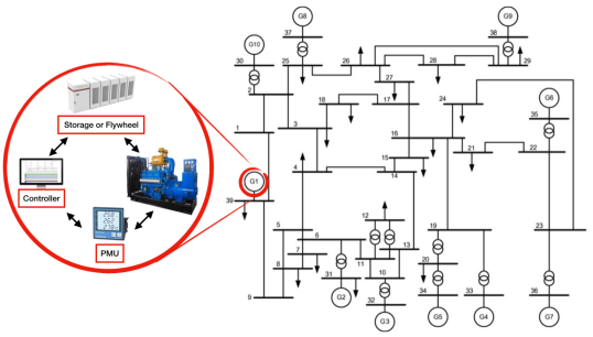
Figure 1: IEEE 10-generator 39-bus power system network (figure is adapted from Atawi (2013)). In Example 1, we assume that each generator has both frequency and angle sensors (e.g., PMUs) and also actuator (e.g., storage or flyweel).

6 Numerical Examples

In this section, we consider a numerical example to demonstrate our results.

Example 1 (Power Network).

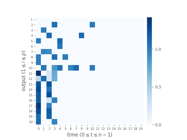
(a)

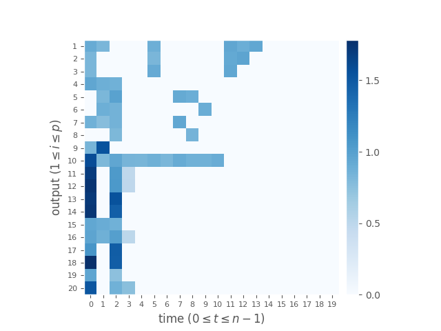
(b)

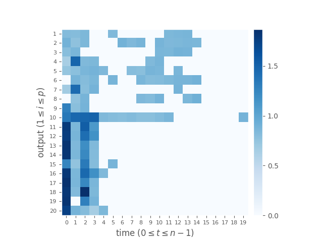
(c)

Figure 2: Subplots (a)-(c) present three weighted sparse sensor schedules for Example 1 based on the proposed deterministic method (Algorithm 2) where $d_{s}\in\{2.2,3.4,6.05\}$ is the average number of active sensors, respectively. The color of element $(i,k)$ is proportional to the scaling factor $\mathfrak{s}^{2}_{i}(k)$ where $i\in[20]$ and $k+1\in[20]$.

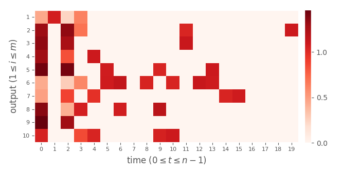
(a)

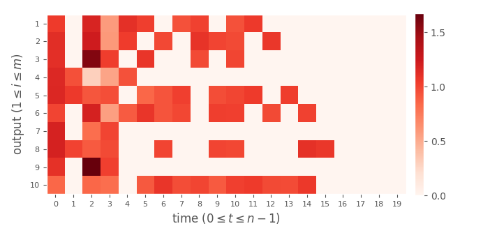
(b)

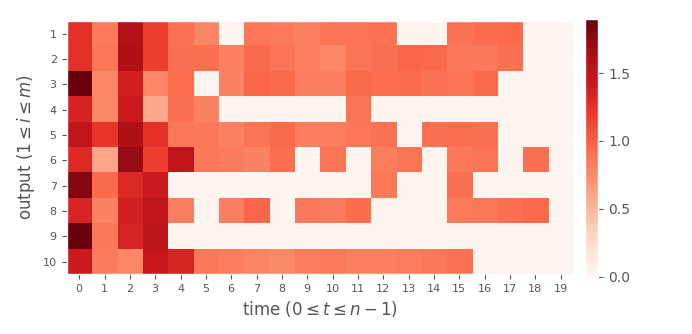
(c)

Figure 3: Subplots (a)-(c) present three weighted sparse actuator schedules for Example 1 based on the proposed deterministic method (Algorithm 2) where $d_{a}\in\{2.3,3.95,6.35\}$ is the average number of active actuators, respectively. The color of element $(i,k)$ is proportional to the scaling factor $\mathfrak{a}^{2}_{i}(k)$ where $i\in[20]$ and $k+1\in[20]$.

The problem is to select a set of sensors and actuators to be involved in the wide-area damping control of power systems. We apply our sparse scheduling approach on the IEEE 39-bus test system (a.k.a. the 10-machine New England Power System; see Fig. 1) (Atawi, 2013; Liu et al., 2017). The single line diagram presented in this figure comprises generators ($G_{i}$ where $i\in[10]$), loads (arrows), transformers (double circles), buses (bold line segments with number $i\in[39]$), and lines between buses (see Atawi (2013); Liu et al. (2017)).

The goal of the wide-area damping control is to damp the fluctuations between generators and synchronize all generators. The voltage at each generator is adjusted by the control inputs to regulate the power output.

We start with a model representing the interconnection between subsystems. Consider the continuous-time swing dynamics

$$m_{i}\ddot{\theta_{i}}+d_{i}\dot{\theta_{i}}~{}=~{}-\sum_{j\sim i}k_{ij}(\theta_{i}-\theta_{j})+u_{i},$$

where $\theta_{i}$ is the rotor angle state and $w_{i}:=\dot{\theta}_{i}$ is the frequency state of generator $i$. We assume this power grid model consists of $n=10$ generators (Liu et al., 2017; Atawi, 2013). The state space model of the swing equation used for frequency control in power networks can be written as follows

$$\left[\begin{array}[]{ccc}\dot{\theta}(t)\\ \dot{w}(t)\end{array}\right] = \left[\begin{array}[]{ccc}0&I\\ -M^{-1}L&-M^{-1}D\end{array}\right]\left[\begin{array}[]{ccc}\theta(t)\\ w(t)\end{array}\right]$$

$$~{}+~{}\left[\begin{array}[]{ccc}0\\ M^{-1}\end{array}\right]u(t)$$

$$y(t) = \left[\begin{array}[]{ccc}\theta(t)\\ w(t)\end{array}\right],$$

where $M$ and $D$ are diagonal matrices with inertia coefficients and damping coefficients of generators and their diagonals, respectively.

We assume that both rotor angle and frequency are available for measurement at each generator. This means each subsystem in the power network has a phase measurement unit (PMU). The PMU is a device that measures the electrical waves on an electricity grid using a common time source for synchronization. The system is discretized to the discrete-time LTI system with state matrices $A$, $B$, and $C$ and the sampling time of $0.2$ second (the matrices are borrowed from Fazelnia et al. (2017)).

Table 1: The values of approximation factor $\epsilon$ for 20 different (S/A) schedules based on Algorithm 2 for the power system given in Example 1. Parameters $d_{\text{s}}$ and $d_{\text{a}}$ are defined by (24) and (25), respectively. The last column (in cyan color) shows the value of approximation factor $\epsilon$ for 5 different sensor schedules where all actuators are active (see Definition 1), and the last row (in blue color) shows the value of approximation factor $\epsilon$ for 4 different actuator schedules where all sensors are active (see Definition 2). Moreover, this table validates Theorem 3 as the sum of approximation factors for the two separate sensor and actuator scheduling problems is greater than the approximation factor for the joint S/A schedule and the gap is small.

		Average Number of Active Actuators
		$d_{\text{a}}=2.3$	$d_{\text{a}}=3.95$	$d_{\text{a}}=6.35$	Fully actuated
Avg.# Active Sensors	$d_{\text{s}}=2.2$	${\bf 4.1330}<{\color[rgb]{0,0,1}1.9434}+{\color[rgb]{0,1,1}2.3281}$	${\bf 3.4365}<{\color[rgb]{0,0,1}1.2366}+{\color[rgb]{0,1,1}2.3281}$	${\bf 2.9078}<{\color[rgb]{0,0,1}0.6983}+{\color[rgb]{0,1,1}2.3281}$	$2.3281$
	$d_{\text{s}}=3.4$	${\bf 3.4794}<{\color[rgb]{0,0,1}1.9434}+{\color[rgb]{0,1,1}1.7157}$	${\bf 2.7821}<{\color[rgb]{0,0,1}1.2366}+{\color[rgb]{0,1,1}1.7157}$	${\bf 2.2595}<{\color[rgb]{0,0,1}0.6983}+{\color[rgb]{0,1,1}1.7157}$	$1.7157$
	$d_{\text{s}}=6.05$	${\bf 2.8551}<{\color[rgb]{0,0,1}1.9434}+{\color[rgb]{0,1,1}1.0691}$	${\bf 2.1545}<{\color[rgb]{0,0,1}1.2366}+{\color[rgb]{0,1,1}1.0691}$	${\bf 1.6316}<{\color[rgb]{0,0,1}0.6983}+{\color[rgb]{0,1,1}1.0691}$	$1.0691$
	$d_{\text{s}}=8.85$	${\bf 2.4421}<{\color[rgb]{0,0,1}1.9434}+{\color[rgb]{0,1,1}0.6399}$	${\bf 1.7370}<{\color[rgb]{0,0,1}1.2366}+{\color[rgb]{0,1,1}0.6399}$	${\bf 1.2107}<{\color[rgb]{0,0,1}0.6983}+{\color[rgb]{0,1,1}0.6399}$	$0.6399$
	Fully sensed	$1.9434$	$1.2366$	$0.6983$	$0$

Figs. 2 and 3 depict joint sparse sensor and actuator schedules based on the proposed deterministic method (Algorithms 2) for different values of $d_{\text{s}}$ and $d_{\text{a}}$.

To have a fair comparison, we normalize the resulting schedules such that the sum of all the scalings satisfies

$$\sum_{k=0}^{n-1}\sum_{i=1}^{p}\mathfrak{s}_{i}^{2}(k)=nd_{\text{s}},$$

and

$$\sum_{k=0}^{n-1}\sum_{i=1}^{m}\mathfrak{a}_{i}^{2}(k)=nd_{\text{a}},$$

where $d_{\text{s}}$ and $d_{\text{a}}$ are average numbers of active sensors and actuators, respectively.

In Table 1, the values of approximation factor $\epsilon$ for 20 different (S/A) schedules based on Algorithm 2 for the power system given in Example 1. The last column (in cyan color) shows the value of approximation factor $\epsilon$ for 5 different sensor schedules where all actuators are active (see Definition 1) and the last row (in blue color) shows the value of approximation factor $\epsilon$ for 4 different actuator schedules where all sensors are active (see Definition 2). Based on Theorem 3 the $(\epsilon,d_{\text{s}},d_{\text{a}})$-joint S/A schedule can be obtained by designing two separate sensor and actuator schedules. This can be validated by Table 1, as the sum of approximation factors for the two separate sensor and actuator scheduling problems is greater than the approximation factor for the joint S/A schedule. For example, based on Table 1, by combining $(1.0691,6.35)$-actuator schedule and $(0.6983,6.05)$-actuator schedule, we get joint $(1.6316,6.35,6.05)$-S/A schedule. We should note that $1.6316<1.0691+0.6983=1.7674$; therefore, it follows that this joint schedule is also $(1.7674,6.35,6.05)$-S/A schedule (cf. Theorem 3).

Table 2: The values of Hankel norm $\sigma_{\max}(\mathcal{H}_{s})$ for 20 different (S/A) schedules based on Algorithm 2 for the power system given in Example 1. Parameters $d_{\text{s}}$ and $d_{\text{a}}$ show average numbers of active sensors and actuators, respectively. For example, $0.1607$ is the value of Hankel norm of the (S/A) schedule with on average $d_{\text{s}}=2.2$ active sensors and $d_{\text{a}}=3.95$ active actuators.

		Average Number of Active Actuators
		$d_{\text{a}}=2.3$	$d_{\text{a}}=3.95$	$d_{\text{a}}=6.35$	$d_{\text{a}}=10$
Avg.# Active Sensors	$d_{\text{s}}=2.2$	$0.1297$	$0.1607$	$0.2020$	$0.2521$
	$d_{\text{s}}=3.4$	$0.1672$	$0.2134$	$0.2697$	0.3429
	$d_{\text{s}}=6.05$	$0.2271$	$0.2935$	$0.3718$	0.4714
	$d_{\text{s}}=8.85$	$0.2800$	$0.3632$	$0.4602$	$0.5838$
	$d_{\text{s}}=20$	$0.3790$	$0.4981$	$0.6322$	$0.8036$

Table 3: The values of $|\log(\frac{\sigma_{\max}(\mathcal{H}_{s})}{\sigma_{\max}(\mathcal{H})})|$ for 20 different (S/A) schedules based on Algorithm 2 for the power system given in Example 1. The matrix $\mathcal{H}_{s}$ and $\mathcal{H}$ are the Hankel matrices of (1)-(2) and (18)-(19), respectively. Parameters $d_{\text{s}}$ and $d_{\text{a}}$ are defined by (24) and (25), respectively. For example, $|\log(\frac{\sigma_{\max}(\mathcal{H}_{s})}{\sigma_{\max}(\mathcal{H})})|=0.7706$ for the (S/A) schedule with on average $d_{\text{s}}=6.05$ active sensors and $d_{\text{a}}=6.35$ active actuators.

		Average Number of Active Actuators
		$d_{\text{a}}=2.3$	$d_{\text{a}}=3.95$	$d_{\text{a}}=6.35$	$d_{\text{a}}=10$
Avg.# Active Sensors	$d_{\text{s}}=2.2$	$1.8237$	$1.6094$	$1.3808$	$1.1592$
	$d_{\text{s}}=3.4$	$1.5698$	$1.3260$	$1.0918$	$0.8515$
	$d_{\text{s}}=6.05$	$1.2634$	$1.0070$	$0.7706$	$0.5333$
	$d_{\text{s}}=8.85$	$1.0543$	$0.7940$	$0.5573$	$0.3194$
	$d_{\text{s}}=20$	$0.7515$	$0.4783$	$0.2399$	$0$

In Tables 2 and 3, the values of Hankel norm $\sigma_{\max}(\mathcal{H}_{s})$ and relative error $|\log(\frac{\sigma_{\max}(\mathcal{H}_{s})}{\sigma_{\max}(\mathcal{H})})|$ for 20 different (S/A) schedules are calculated based on Algorithm 2, respectively.

The sparsity degree of each schedule is captured by $d_{\text{s}}$ and $d_{\text{a}}$. Based on Table 2, as parameter $d_{\text{a}}$ (i.e., the average number of active actuators) increases both the number of non-zero scalings (i.e., activations) and the Hankel norm increase. Similarly, as parameter $d_{\text{s}}$ (i.e., the average number of active sensors) increases both the number of non-zero scalings (i.e., activations) and the Hankel norm increase. As one expects, according to Table 3, the value of $|\log(\frac{\sigma_{\max}(\mathcal{H}_{s})}{\sigma_{\max}(\mathcal{H})})|$ decreases as the number of active sensors or actuators increases.

Finally, we should note that the value of $|\log(\frac{\sigma_{\max}(\mathcal{H}_{s})}{\sigma_{\max}(\mathcal{H})})|$ is less than the value of corresponding approximation factor $\epsilon$ (cf. Tables 1 and 3). The values of $|\log(\frac{\rho(\mathcal{H}_{s})}{\rho(\mathcal{H})})|$ in fact is less than $\epsilon$ for any Hankel-based performance measures based on Definition 3 and (17).

7 Concluding Remarks

In this paper, we studied the problem of designing a joint sparse sensor and actuator (S/A) schedule of linear dynamical systems that retains the full observability and controllability of the system. Based on recent advances in matrix reconstruction and graph sparsification literature, we provide a polynomial-time joint S/A schedule for a discrete time linear dynamical system. This joint S/A schedule on average selects only a constant number of sensors and actuators at each time step, while guaranteeing a control/estimation performance that approximates the fully sensed/actuated setting. We further prove the validity of separation principle for the system, showing that the problem can be decomposed into finding sensor and actuator schedules separately.

References

• (1)
• Allen-Zhu et al. (2017) Allen-Zhu, Z., Y. Li, A. Singh and Y. Wang (2017). Near-optimal design of experiments via regret minimization. In: Proceedings of the 34th International Conference on Machine Learning. Vol. 70. PMLR. pp. 126–135.
• Antoulas (2005) Antoulas, A. C. (2005). Approximation of large-scale dynamical systems. Vol. 6. Siam.
• Argha et al. (2017) Argha, A., S. W. Su, A. Savkin and B. Celler (2017). A framework for optimal actuator/sensor selection in a control system. International Journal of Control pp. 1–19.
• Atawi (2013) Atawi, I. E. (2013). An advance distributed control design for wide-area power system stability. PhD thesis. University of Pittsburgh.
• Athans (1972) Athans, M. (1972). On the determination of optimal costly measurement strategies for linear stochastic systems. Automatica 8(4), 397–412.
• Bopardikar (2017) Bopardikar, S. D. (2017). Sensor selection via randomized sampling. arXiv preprint arXiv:1712.06511.
• Boutsidis et al. (2014) Boutsidis, C., P. Drineas and M. Magdon-Ismail (2014). Near-optimal column-based matrix reconstruction. SIAM Journal on Computing 43(2), 687–717.
• Chakrabortty and Ilić (2011) Chakrabortty, A. and M. D. Ilić (2011). Control and optimization methods for electric smart grids. Vol. 3. Springer.
• Chandra et al. (2011) Chandra, F. A., G. Buzi and J.C. Doyle (2011). Glycolytic oscillations and limits on robust efficiency. Science 333(6039), 187–192.
• Chanekar et al. (2017) Chanekar, P. V., N. Chopra and S. Azarm (2017). Optimal actuator placement for linear systems with limited number of actuators. In: 2017 American Control Conference (ACC). pp. 334–339.
• Fahroo and Demetriou (2000) Fahroo, F. and M. A. Demetriou (2000). Optimal actuator/sensor location for active noise regulator and tracking control problems. Journal of Computational and Applied Mathematics 114(1), 137–158.
• Fazelnia et al. (2017) Fazelnia, G., R. Madani, A. Kalbat and J. Lavaei (2017). Convex relaxation for optimal distributed control problems. IEEE Transactions on Automatic Control 62(1), 206–221.
• Glover (1987) Glover, K. (1987). Model reduction: a tutorial on hankel-norm methods and lower bounds on $L_{2}$ errors. IFAC Proceedings Volumes 20(5), 293–298.
• Jadbabaie et al. (2018a) Jadbabaie, A., A. Olshevsky and M. Siami (2018a). Deterministic and randomized actuator scheduling with guaranteed performance bounds. arXiv preprint arXiv:1805.00606.
• Jadbabaie et al. (2018b) Jadbabaie, A., A. Olshevsky and M. Siami (2018b). Limitations and tradeoffs in minimum input selection problems. In: 2018 Annual American Control Conference, ACC 2018, Milwaukee, WI, USA, June 27-29, 2018. pp. 185–190.
• Jadbabaie et al. (2019) Jadbabaie, A., A. Olshevsky, G. J. Pappas and V. Tzoumas (2019). Minimal reachability is hard to approximate. IEEE Transactions on Automatic Control 64(2), 783–789.
• Kempthorne (1952) Kempthorne, O. (1952). The design and analysis of experiments.. Wiley.
• Liu and Barabási (2016) Liu, YY and AL Barabási (2016). Control principles of complex systems. Reviews of Modern Physics 88(3), 035006.
• Liu et al. (2017) Liu, Z., Y. Long, A. Clark, P. Lee, L. Bushnell, D. Kirschen and R. Poovendran (2017). Minimal input selection for robust control. arXiv preprint arXiv:1712.01232.
• Marcus et al. (2015) Marcus, A. W., D. A. Spielman and N. Srivastava (2015). Interlacing families ii: Mixed characteristic polynomials and the kadison-singer problem. Annals of Mathematics pp. 327–350.
• Marucci et al. (2009) Marucci, L., D. AW Barton, I. Cantone, M. A. Ricci, M. P. Cosma, S. Santini, D. di Bernardo and M. di Bernardo (2009). How to turn a genetic circuit into a synthetic tunable oscillator, or a bistable switch. PLoS One 4(12), e8083.
• Matni and Chandrasekaran (2016) Matni, N. and V. Chandrasekaran (2016). Regularization for design. IEEE Transactions on Automatic Control 61(12), 3991–4006.
• Moore (1981) Moore, B. (1981). Principal component analysis in linear systems: Controllability, observability, and model reduction. IEEE Transactions on Automatic Control 26(1), 17–32.
• Müller and Weber (1972) Müller, PC and HI Weber (1972). Analysis and optimization of certain qualities of controllability and observability for linear dynamical systems. Automatica 8(3), 237–246.
• Nozari et al. (2017) Nozari, E., F. Pasqualetti and J. Cortés (2017). Time-invariant versus time-varying actuator scheduling in complex networks. In: 2017 American Control Conference (ACC). pp. 4995–5000.
• Nozari et al. (2019) Nozari, E., F. Pasqualetti and J. Cortés (2019). Heterogeneity of central nodes explains the benefits of time-varying control scheduling in complex dynamical networks. Journal of Complex Networks.
• Olshevsky (2014) Olshevsky, A. (2014). Minimal controllability problems. IEEE Transactions on Control of Network Systems 1(3), 249–258.
• Olshevsky (2015) Olshevsky, A. (2015). Minimum input selection for structural controllability. In: 2015 American Control Conference (ACC). pp. 2218–2223.
• Pasqualetti et al. (2014) Pasqualetti, F., S. Zampieri and F. Bullo (2014). Controllability metrics, limitations and algorithms for complex networks. IEEE Transactions on Control of Network Systems 1(1), 40–52.
• Pequito et al. (2017) Pequito, S., G. Ramos, S. Kar, A. P. Aguiar and J. Ramos (2017). The robust minimal controllability problem. Automatica 82, 261 – 268.
• Pequito et al. (2015) Pequito, S., S. Kar and A. P. Aguiar (2015). On the complexity of the constrained input selection problem for structural linear systems. Automatica 62, 193–199.
• Rajapakse et al. (2012) Rajapakse, I., M. Groudine and M. Mesbahi (2012). What can systems theory of networks offer to biology?. PLoS computational biology 8(6), e1002543.
• Ravi et al. (2016) Ravi, S. N., V. Ithapu, S. Johnson and V. Singh (2016). Experimental design on a budget for sparse linear models and applications. In: International Conference on Machine Learning. pp. 583–592.
• Siami and Jadbabaie (2019) Siami, M. and A. Jadbabaie (2019). A separation principle for joint sensor and actuator scheduling with guaranteed performance bounds. IEEE Conference on Decision and Control, submitted.
• Siami and Skaf (2018) Siami, M. and J. Skaf (2018). Structural analysis and optimal design of distributed system throttlers. IEEE Transactions on Automatic Control 63(12), 540–547.
• Siami and Motee (2018) Siami, M. and N. Motee (2018). Network abstraction with guaranteed performance bounds. IEEE Transactions on Automatic Control.
• Summers et al. (2016) Summers, T. H., F. L. Cortesi and J. Lygeros (2016). On submodularity and controllability in complex dynamical networks. IEEE Transactions on Control of Network Systems 3(1), 91–101.
• Tzoumas et al. (2018) Tzoumas, V., L. Carlone, G. J. Pappas and A. Jadbabaie (2018). Sensing-constrained LQG control. In: 2018 Annual American Control Conference (ACC). IEEE. pp. 197–202.
• Tzoumas et al. (2016a) Tzoumas, V., M. A. Rahimian, G. J. Pappas and A. Jadbabaie (2016a). Minimal actuator placement with bounds on control effort. IEEE Transactions Control of Network Systems 3(1), 67–78.
• Tzoumas et al. (2016b) Tzoumas, V., M. A. Rahimian, G. J. Pappas and A. Jadbabaie (2016b). Minimal actuator placement with bounds on control effort. IEEE Transactions on Control of Network Systems 3(1), 67–78.
• Yazıcıoğlu et al. (2016) Yazıcıoğlu, A. Y., W. Abbas and M. Egerstedt (2016). Graph distances and controllability of networks. IEEE Transactions on Automatic Control 61(12), 4125–4130.