Exponential decay for negative feedback loop with distributed delay

Abstract

We derive sufficient conditions for exponential decay of solutions of the delay negative feedback equation with distributed delay. The conditions are written in terms of exponential moments of the distribution. Our method only uses elementary tools of calculus and is robust towards possible extensions to more complex settings, in particular, systems of delay differential equations. We illustrate the applicability of the method to particular distributions - Dirac delta, Gamma distribution, uniform and truncated normal distributions.

Keywords: Negative feedback loop, distributed delay, exponential decay.

2010 MR Subject Classification: 34K06, 34K25, 34K11.

1 Introduction and main result

In this paper we derive sufficient conditions for exponential decay of solutions of the delay negative feedback equation with distributed delay,

$$\dot{u}(t)=-F_{P}[u](t):=-\int_{0}^{\infty}u(t-s)\mathrm{d}{P}(s)\qquad\mbox{for }t>0,$$ (1)

where $P$ is a probability measure on $[0,\infty)$. Note that the normalization $\int_{0}^{\infty}\mathrm{d}P=1$ can be imposed by an eventual rescaling of the time variable. For simplicity, we consider (1) subject to the constant initial datum $u(s)\equiv 1$ for $s\leq 0$; alternatively, we may assume that (1) holds globally, i.e., for all $t\in\mathbb{R}$.

The importance of equation (1), also called a linear retarded functional differential equation, stems from the fact that it can be seen as a linearization of many nonlinear models in biology and physics involving delay. As such, it has been a long-standing subject of interest of the mathematical community. Basic theory for delay differential equations and functional differential equations can be found in, e.g., [3] and [9], while [7] and [13] focus on applications. The theory typically focuses on two qualitative aspects of delay/functional differential equations - (asymptotic) stability of the steady state solutions [6, 11], and oscillatory behavior [1, 2, 4, 12]. This note aims to contribute to the study of the latter aspect by deriving sufficient conditions for the solution of (1) to decay monotonically (exponentially) to zero. In contrast to the traditional approach, based on studying the characteristic equation, our method only uses elementary tools of calculus. It provides relatively simple sufficient conditions for exponential decay of the solution, written in terms of the exponential moments of the distribution $P$. Due to its simplicity, it can be applied to systems of delay differential equations, where the analysis of the characteristic equation would be prohibitively complex; see [10] for a recent application. Let us note that in the case when $P$ is a Dirac measure, a slight modification of the method leads to an optimal (i.e., equivalent) condition for monotone decay of the solution.

In the sequel we shall denote, for $\mu>0$, the exponential moment of $p$ by

$$\mathbb{M}_{P}(\mu):=\int_{0}^{\infty}e^{\mu s}\mathrm{d}P(s).$$ (2)

Theorem 1.

If there exists some $\mu>1$ such that

$$\mathbb{M}_{P}(2\mu)\leq\mu^{2}$$ (3)

and

$${\mathbb{M}_{P}(\mu)}(\mathbb{M}_{P}(\mu)-1)<\mu,$$ (4)

then the solution $u=u(t)$ of (1) converges monotonically exponentially to zero as $t\to\infty$ with rate at least

$$2\left(\frac{\mathbb{M}_{P}(\mu)\bigl{(}\mathbb{M}_{P}(\mu)-1\bigr{)}}{\mu}-1\right).$$

Let us note that in the standard theory (1) is called nonoscillatory if there exists an initial datum $u_{0}$ such that the solution of the initial value problem is eventually positive or eventually negative (see Definition 1.1 in [1]). Therefore, Theorem 1 provides sufficient conditions for (1) to be nonoscillatory. Let us again point out the relative simplicity of the conditions (3), (4), being only written in terms of the exponential moments of the distribution $P$.

The proof of Theorem 1 is based on suitable decay estimates for the quantity $y(t):=u^{2}(t)/2$ and is carried out in Section 2. In Section 3 we show the applicability of the result to particular choices of the measure $P$. First, we consider the Dirac measure concentrated at $\tau>0$, $P(s)=\delta(s-\tau)$, which turns (1) into the simple negative feedback equation with constant delay $\tau>0$,

$$\dot{u}(t)=-u(t-\tau)\qquad\mbox{for }t>0.$$ (5)

We shall show that the conditions (3) and (4) are satisfied if

$$\tau<\ln\sqrt{2}.$$

Moreover, we shall show that by a slight modification of the proof of Theorem 1 we obtain monotone decay of the solution as soon as $\tau\leq e^{-1}$. This result is sharp since it is known that for $\tau>e^{-1}$ the nontrivial solutions of (5) must oscillate [8]. The second example is the Gamma distribution $\mathrm{d}P(s)=\lambda^{k}s^{k-1}e^{-\lambda s}/\Gamma(k)$ with shape parameter $k>0$ and rate parameter $\lambda>0$. Here we derive explicit sufficient conditions for satisfiability of (3), (4). In the special case of $k=1$, which corresponds to the exponential distribution, we show that the solution is nonoscillatory if $\lambda\geq 3^{\frac{3}{2}}\approx 5.196$. The optimal condition for nonoscillation is $\lambda\geq 4$, see [5]. Finally, for the uniform and truncated normal distributions we resolve the conditions (3), (4) numerically.

2 Proof of the main result

In this section we assume that $u=u(t)$ is a solution of (1) subject to the constant initial datum, and we introduce the notation

$$y(t) := u^{2}(t)/2\qquad\mbox{for }t\geq 0,$$

$$:= u_{0}^{2}(t)/2\qquad\mbox{for }t<0.$$

Lemma 1.

If assumption (3) is verified for some $\mu>1$, then for all $t>0$ and $s>0$,

$$e^{-2\mu s}y(t)<y(t-s)<e^{2\mu s}y(t).$$ (7)

Proof.

We have

$$\left|\frac{\dot{y}(0+)}{y(0)}\right|=2\left|\frac{\dot{u}(0+)}{u(0)}\right|=2\left|\frac{F_{P}[u](0)}{u(0)}\right|=2<2\mu.$$

Due to the continuity of $\dot{y}(t)$ for $t>0$, there exists $T>0$ such that

$$\left|\frac{\dot{y}(t)}{y(t)}\right|<2\mu\qquad\mbox{for }t<T.$$ (8)

We claim that (8) holds for all $t\in\mathbb{R}$, i.e., $T=+\infty$. For contradiction, assume that $T<+\infty$, then again by continuity we have

$$|\dot{y}(T)|=2\mu y(T).$$ (9)

Integrating (8) on the time interval $(T-s,T)$ with $s>0$ yields

$$y(T-s)<e^{2\mu s}y(T).$$ (10)

Consequently,

$$F_{P}[y](T)=\int_{0}^{\infty}y(T-s)\mathrm{d}P(s)<y(T)\int_{0}^{\infty}e^{2\mu s}\mathrm{d}P(s)=y(T)\mathbb{M}_{P}(2\mu).$$ (11)

Using the Young inequality with some $\varepsilon>0$, we have

$$|\dot{y}(T)|=|u(T)F_{P}[u](T)|\leq\frac{\varepsilon}{2}u(T)^{2}+\frac{1}{2\varepsilon}\bigl{(}F_{P}[u](T)\bigr{)}^{2}$$

and with Jensen inequality

$$\frac{1}{2\varepsilon}\bigl{(}F_{P}[u](T)\bigr{)}^{2}=\frac{1}{2\varepsilon}\left(\int_{0}^{\infty}u(T-s)\mathrm{d}P(s)\right)^{2}\leq\frac{1}{2\varepsilon}\int_{0}^{\infty}u(T-s)^{2}\mathrm{d}P(s)=\frac{1}{\varepsilon}F_{P}[y](T).$$

Consequently, with (11) we arrive at

$$|\dot{y}(T)|\leq y(T)\left(\varepsilon+\frac{1}{\varepsilon}\mathbb{M}_{P}(2\mu)\right)$$

Optimization in $\varepsilon>0$ gives $\varepsilon:=\sqrt{\mathbb{M}_{P}(2\mu)}$, so that we have

$$|\dot{y}(T)|<2y(T)\sqrt{\mathbb{M}_{P}(2\mu)},$$

and, with assumption (3) we finally arrive at

$$|\dot{y}(T)|<2\mu y(T),$$

a contradiction to (9). Consequently, (8) holds with $T:=\infty$, and an integration on the interval $(t-s,t)$ implies (7). ∎

Lemma 2.

If assumptions (3) and (4) are verified for some $\mu>1$, then we have, along the solutions of (1),

$$\dot{y}(t)<2\left(\frac{\mathbb{M}_{P}(\mu)\bigl{(}\mathbb{M}_{P}(\mu)-1\bigr{)}}{\mu}-1\right)y(t)$$ (12)

for all $t>0$.

Proof.

For $t>0$ we have

$$\dot{y}=-uF_{P}[u]=(u-F_{P}[u])u-u^{2}\leq|u-F_{P}[u]||u|-u^{2},$$ (13)

and

$$|u(t)-F_{P}[u](t)|\leq\int_{0}^{\infty}|u(t)-u(t-s)|\mathrm{d}P(s).$$ (14)

With (1) we have

$$|u(t)-u(t-s)|\leq\int_{t-s}^{t}|\dot{u}(\sigma)|\mathrm{d}\sigma\leq\int_{t-s}^{t}|F_{P}[u](\sigma)|\mathrm{d}\sigma,$$

and with Lemma 1,

$$|F_{P}[u](\sigma)|\leq\int_{0}^{\infty}|u(\sigma-\theta)|\mathrm{d}P(\theta)<|u(\sigma)|\int_{0}^{\infty}e^{\mu\theta}\mathrm{d}P(\theta)=|u(\sigma)|\mathbb{M}_{P}(\mu).$$

Using Lemma 1 again, we obtain

$$\int_{t-s}^{t}|F_{P}[u](\sigma)|\mathrm{d}\sigma < \mathbb{M}_{P}(\mu)\int_{t-s}^{t}|u(\sigma)|\mathrm{d}\sigma$$

$$< \mathbb{M}_{P}(\mu)|u(t)|\int_{0}^{s}e^{\mu\theta}\mathrm{d}\theta=\frac{\mathbb{M}_{P}(\mu)}{\mu}\left(e^{\mu s}-1\right)|u(t)|,$$

and inserting into (14),

$$|u(t)-F_{P}[u](t)|<\frac{\mathbb{M}_{P}(\mu)\bigl{(}\mathbb{M}_{P}(\mu)-1\bigr{)}}{\mu}|u(t)|.$$

Using this in (13) gives

$$\dot{y}(t)<\left(\frac{\mathbb{M}_{P}(\mu)\bigl{(}\mathbb{M}_{P}(\mu)-1\bigr{)}}{\mu}-1\right)u^{2}(t)$$

and (12) follows. ∎

The statement of Theorem 1 follows directly from the above two Lemmata. Let us note that the above proofs apply without modification also to the case of global solutions, where (1) holds on the whole real line.

3 Application to generic distributions

We show the application of Theorem 1 to the Dirac delta and exponential distribution, where it provides explicit conditions for monotone decay of the solution.

3.1 Dirac delta.

We choose $P(s)=\delta(s-\tau)$ for a fixed $\tau>0$. Then $F_{P}[u](t)=u(t-\tau)$ and (1) transforms to the negative feedback loop with constant delay,

$$\dot{u}(t)=-u(t-\tau).$$ (15)

Delay negative feedback is arguably the simplest nontrivial delay differential equation. Despite its simplicity, it exhibits a surprisingly rich qualitative dynamics, depending on the value of $\tau>0$. An analysis of the corresponding characteristic equation

$$z+\tau e^{-z}=0,$$

where $z\in\mathbb{C}$, reveals that:

• If $0<\tau\leq e^{-1}$, then $u=0$ is asymptotically stable.

• If $e^{-1}<\tau<\pi/2$, then $u=0$ is asymptotically stable, but every nontrivial solution of (15) is oscillatory.

• If $\tau=\pi/2$, then periodic solutions exist.

• If $\tau>\pi/2$, then $u=0$ is unstable.

In fact, if $\tau\leq e^{-1}$, the solutions subject to the constant initial datum do not oscillate and tend monotonically to zero as $t\to\infty$. If $\tau$ becomes larger than $e^{-1}$ but smaller than $\pi/2$, the nontrivial solutions must oscillate (i.e., change sign infinitely many times as $t\to\infty$), but the oscillations are damped and vanish as $t\to\infty$. Finally, for $\tau>\pi/2$ the nontrivial solutions oscillate with unbounded amplitude as $t\to\infty$. We refer to Chapter 2 of [13] and [8] for details.

With $P(s)=\delta(s-\tau)$ we readily have $\mathbb{M}_{P}[\mu]=e^{\mu\tau}$ and condition (3) reads

$$e^{\mu\tau}\leq\mu.$$

A simple analysis reveals that this condition is satisfiable if and only if $\tau\leq e^{-1}$ and that for $\tau=e^{-1}$ we have to choose $\mu=e$. However, condition (4) is more restrictive, since for $\tau=e^{-1}$, $\mu=e$ it reads $e(e-1)<e$ and clearly is not satisfied. Since the left-hand side of (4) grows exponentially in $\mu\tau$, we are motivated to pick $\mu$ as the solution of $\mu=e^{\mu\tau}$. Inserting into (4) gives then

$$\mu\left(\mu-1\right)<\mu,$$

i.e., $\mu<2$. Going back to (3) with $\mu=2$, we obtain the critical value of $\tau=\ln\sqrt{2}\approx 0.3466$. This is less optimal than the condition $\tau<e^{-1}\approx 0.3679$ by factor of approx. $0.94$. However, let us note that with a slight modification of the proof of Lemma 2 we can obtain monotone decay of the solution to zero for all $\tau\leq e^{-1}$. Indeed, we replace (13) by

$$\dot{y}=-uF_{P}[u]\leq|u-F_{P}[u]||F_{P}[u]|-F_{P}[u]^{2},$$ (16)

and, restricting to $t>\tau$,

$$|u(t)-F_{P}[u](t)|=|u(t)-u(t-\tau)| \leq \int_{t-\tau}^{t}|\dot{u}(s)|\mathrm{d}s$$ (17)

$$\leq \int_{t-\tau}^{t}|u(s-\tau)|\mathrm{d}s=\int_{-\tau}^{0}|u(t+s-\tau)|\mathrm{d}s.$$ (18)

Using Lemma 1 with $\mu:=e$ we obtain $|u(t-\tau+s)|<e^{-es}|u(t-\tau)|$ for $s\in(-\tau,0)$, which gives

$$|u(t)-F_{P}[u](t)|<|u(t-\tau)|\int_{0}^{\tau}e^{es}\mathrm{d}s=\frac{e^{e\tau}-1}{e}|u(t-\tau)|.$$

Therefore, recalling that $F_{P}[u](t)=u(t-\tau)$, we have for $t>\tau$,

$$\dot{y}<\left(\frac{e^{e\tau}-1}{e}-1\right)F_{P}[u]^{2}.$$ (19)

Consequently, for $\tau\leq e^{-1}$ we readily have $\dot{y}<-e^{-1}F_{P}[u]^{2}\leq 0$ for all $t>\tau$, and we conclude that $y=y(t)$, and thus $u=u(t)$, tend monotonically to zero as $t\to\infty$. Let us point out that this result is sharp since we know that if $\tau>e^{-1}$, the solution must oscillate [8].

3.2 Gamma distribution.

For the Gamma distribution $\mathrm{d}P(s)=\lambda^{k}s^{k-1}e^{-\lambda s}/\Gamma(k)$ with shape parameter $k>0$ and rate parameter $\lambda>0$ we have for $\mu<\lambda$,

$$\mathbb{M}_{P}[\mu]=\left(\frac{\lambda}{\lambda-\mu}\right)^{k}.$$

Condition (3) reads

$$\left(\frac{\lambda}{\lambda-2\mu}\right)^{k}\leq\mu^{2}$$

and is satisfiable if and only if

$$\lambda\geq\frac{(k+2)^{\frac{k+2}{2}}}{k^{\frac{k}{2}}}.$$ (20)

with $\mu:=\frac{\lambda}{k+2}$. Inserting this value into condition (4), we obtain

$$\frac{[k(k+2)]^{\frac{k}{2}}}{(k+1)^{k}}\left(\left(\frac{k+2}{k+1}\right)^{k}-1\right)<1,$$

and an inspection reveals that this is satisfied for all $k\leq 4$. Consequently, (1) is nonoscillatory (at least) for $k\leq 4$ if $\lambda$ satisfies (20).

Let us point out the special case of $k=1$, which corresponds to the exponential distribution. Condition (20) gives here $\lambda\geq 3^{\frac{3}{2}}\approx 5.196$, while the optimal condition for nonoscillation is $\lambda\geq 4$, see [5].

3.3 Uniform distribution

For $\mathrm{d}P(s)=\frac{1}{b-a}\chi_{[a,b]}(s)\mathrm{d}s$ with $0\leq a<b$ we have

$$\mathbb{M}_{P}[\mu]=\frac{e^{\mu b}-e^{\mu a}}{(b-a)\mu}.$$

Combining the rough estimate

$$e^{\mu a}\leq\mathbb{M}_{P}[\mu]\leq e^{\mu b}$$

with the results of Section 3.1 implies, as expected, that the solution is nonoscillatory whenever $b<\ln\sqrt{2}$. On the other hand, conditions (3), (4) cannot be satisfied if $a>\ln\sqrt{2}\approx 0.3466$. We resolved the conditions (3), (4) numerically, using the matlab routine fminbnd. The resulting critical curve is plotted in Fig. 1. The upper limit on $a$ is approx. $0.346$, in agreement with the analytical result. On the other hand, for values of $a$ close to zero, the interval length $b-a$ can up to approx. $0.59$.

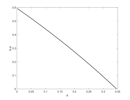
Figure 1: Numerical calculation of the critical value of the interval length $b-a$ as a function of the parameter $a$ for the uniform distribution on $[a,b]$.

3.4 Truncated Gaussian distribution.

For the truncated normal distribution on $(0,\infty)$ with parameters $m\in\mathbb{R}$ and $\sigma>0$ we have

$$\mathrm{d}P(s)=\frac{1}{\sqrt{2\pi\sigma^{2}}}\frac{\exp\left(-\frac{1}{2}\left(\frac{s-m}{\sigma}\right)^{2}\right)}{\Phi\left(\frac{m}{\sigma}\right)}\mathrm{d}s,$$ (21)

and

$$\mathbb{M}_{P}[\mu]=\frac{\Phi\left(\frac{m}{\sigma}+\sigma\mu\right)}{\Phi\left(\frac{m}{\sigma}\right)}\exp\left({m\mu+\frac{\sigma^{2}\mu^{2}}{2}}\right).$$

Since $\mathbb{M}_{P}[\mu]\geq e^{m\mu}$, conditions (3), (4) can only be satisfied if $m\leq\ln\sqrt{2}$. Obviously, as $m\to-\infty$, the critical value of $\sigma$ tends to $+\infty.$ We resolved the conditions (3), (4) numerically for $\mu\in[-\ln\sqrt{2},\ln\sqrt{2}]$, using the matlab procedure fminbnd. The result is shown in Fig. 2, where we plot the critical value of $\sigma$ as a function of the parameter $m$.

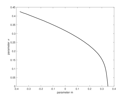
Figure 2: Numerical calculation of the critical value of the parameter $\sigma$ as a function of the parameter $m$ for the truncated normal distribution (21).

References

• [1] R.P. Agarwal, L. Berezansky, E. Braverman and A. Domoshnitsky: Nonoscillation Theory of Functional Differential Equations with Applications. Springer New York Dordrecht Heidelberg London, 2012.
• [2] R.P. Agarwal, S. R. Grace and D. O’Regan: Oscillation Theory for Difference and Functional Differential Equations. Springer-Science+Business Media Dordrecht, 2000.
• [3] R. Bellman and K. Cooke: Differential-difference equations. Academic press, 1963.
• [4] L. Berezansky and E. Braverman: Non-oscillation properties of linear neutral differential equations. Functional Differential Equations 9 (3-4), 2002, pp. 275–288.
• [5] L. Berezansky and E. Braverman: Oscillation of equations with an infinite distributed delay. Computers and Mathematics with Applications 60, 2010, pp. 2583–2593.
• [6] S. Bernard and F. Crauste: Optimal linear stability condition for scalar differential equations with distributed delay. DCDS-B 20(7), 2014.
• [7] T. Erneux: Applied delay differential equations. Springer Verlag, 2009.
• [8] I. Gyori and G. Ladas: Oscillation Theory of Delay Differential Equations with Applications. Oxford Science Publications, Clarendon Press, Oxford, 1991.
• [9] J. Hale and S. Verduyn Lunel: Introduction to functional differential equations. Springer Berlin, 1993.
• [10] J. Haskovec and I. Markou: Asymptotic flocking in the Cucker-Smale model with reaction-type delays in the non-oscillatory regime. To appear in Kin. Rel. Models (2020).
• [11] T. Krizstin: Stability for functional differential equations and some variational problems. Tohoku Math. J. 42, 1990, pp. 407–417.
• [12] G. Ladas, G. Ladde and J.S. Papadakis: Oscillations of functional-differential equations generated by delays. J. Diff. Equ. 12, 1972, pp. 385–395.
• [13] H. Smith: An Introduction to Delay Differential Equations with Applications to the Life Sciences. Springer New York Dordrecht Heidelberg London, 2011.