The Dirac oscillator: an alternative basis for nuclear structure calculations

Abstract

Background: The isotropic harmonic oscillator supplemented by a strong spin-orbit interaction has been the cornerstone of nuclear structure since its inception more than seven decades ago. In this paper we introduce—or rather re-introduced—the “Dirac Oscillator”, a fully relativistic basis that has all the desired attributes of the ordinary harmonic oscillator while naturally incorporating a strong spin-orbit coupling.

Purpose: To assess—to our knowledge for the first time—the power and flexibility of the Dirac Oscillator basis in the solution of nuclear structure problems within the framework of covariant density functional theory.

Methods: Self-consistent calculations of binding energies and ground-state densities for a selected set of doubly-magic magic are performed using the Dirac-oscillator basis and are then compared against results obtained with the often-used Runge-Kutta method.

Results: Results obtained using the Dirac oscillator basis reproduced with high accuracy those derived using the Runge-Kutta method and suggest a clear path for a generalization to systems with axial symmetry.

Conclusions: Although the three-dimensional harmonic oscillator with spin-orbit corrections has been the staple of the nuclear shell model since the beginning, the Dirac oscillator is practically unknown among the nuclear physics community. In this paper we illustrate the power and flexibility of the Dirac oscillator and suggest extensions to the study of systems without spherical symmetry as required in constrained calculations of nuclear excitations.

I Introduction

The isotropic, three-dimensional harmonic oscillator has played a critical role in the development of the nuclear-shell model since its inception in the late 1940s. Indeed, Haxel, Jensen, and Suess start their 1949 seminal paper with: “A simple explanation of the magic numbers 14, 28, 50, 82, 126 follows at once from the oscillator model of the nucleus, if one assumes that the spin-orbit coupling in the Yukawa field theory of nuclear forces leads to a strong splitting …” Haxel et al. (1949). Independently and just two weeks later, Maria Goeppert-Mayer provides detailed evidence supporting the emergence of magic numbers as a consequence of a strong spin-orbit coupling Mayer (1949). In that paper as well as in her 1963 Nobel lectures, Goeppert-Mayer credits Enrico Fermi with a profound insight: “One day as Fermi was leaving my office he asked, Is there any indication of spin-orbit coupling?” Mayer .

Fast forward to today and despite remarkable advances in both refining the underlying interaction and perfecting the many-body methods, the nuclear-structure community continues to rely heavily on the three-dimensional harmonic oscillator with spin-orbit corrections as a convenient and flexible single-particle basis; see Refs. Brown (2001); Dickhoff and Barbieri (2004); Roth et al. (2010); Kortelainen et al. (2010); Hagen et al. (2014); Barrett et al. (2013) and references contained therein for a representative set of modern approaches to nuclear structure. Among the reasons that the harmonic oscillator continues to be heavily used is because it permits a clean separation of the center-of-mass motion and has convenient analytic properties; e.g., it has the same functional form in momentum space as in configuration space.

Although highly successful, relativistic approaches to nuclear structure are more limited in scope and generally fall under the single rubric of covariant density functional theory (DFT) Serot and Walecka (1986); Meng (2016). The aim of covariant DFT is to build high-quality functionals that yield an accurate description of the properties of finite nuclei, generate an equation of state that is consistent with known neutron-star properties, while providing a Lorentz covariant extrapolation to dense matter. However, given that the model parameters underlying the DFT cannot be computed from first principles, their values must be calibrated from a suitable set of experimental data; see Ref. Chen and Piekarewicz (2014) and references contained therein. From such an optimally calibrated density functional, one derives the corresponding Kohn-Sham (or mean-field) equations which are then solved self-consistently Horowitz and Serot (1981). In particular, the nucleon field satisfies a Dirac equation in the presence of strong Lorentz scalar and vector potentials that naturally lead to a very strong spin-orbit splitting. Given that the Dirac equation for spherically symmetric potentials separates into a set of two coupled differential equations in the radial coordinate, one often solves this set of equations using a conventional Runge-Kutta algorithm Horowitz and Serot (1981); Serot and Walecka (1986); Todd and Piekarewicz (2003). Alternatively, one may solve the Dirac equation as a matrix-diagonalization problem by expanding both the upper and lower components of the Dirac spinor in a non-relativistic harmonic oscillator basis; see for example Ref. Meng (2016); Vretenar et al. (2005) and references contained therein. There is, however, a more natural alternative.

Back in 1989 Moshinsky and Szczepaniak modified the free Dirac equation—already linear in the momentum—to one that would be linear in both the coordinates and the momenta of the particle Moshinsky and Szczepaniak (1989); see also a much earlier paper by Itô, Mori, and Carriere Itô et al. (1967). By doing so, they introduced the “The Dirac Oscillator”, a problem that can be solved exactly as both upper and lower components of the Dirac equation satisfy a non-relativistic harmonic oscillator problem with a strong spin-orbit coupling term. Although the paper has generated considerable interest in certain fields, we find surprising that it has not generated as much excitement in the nuclear structure community, given the prominent role that the harmonic oscillator potential supplemented by a strong spin-orbit coupling has played in nuclear physics for so many decades. As we show below, however, the spectrum of the Dirac oscillator is quite different from that of the ordinary non-relativistic harmonic oscillator Quesne and Moshinsky (1990).

The aim of this paper is to introduce and illustrate the value of the Dirac oscillator as a complete basis for the solution of the relativistic Kohn-Sham equations. Comparisons will be made against solutions obtained using the standard Runge-Kutta method. We will also argue in favor of the Dirac oscillator basis over the Runge-Kutta method for the treatment of problems with axial symmetry. The rest of the paper is organized as follows. In Sec. II we briefly review the basic ideas behind covariant DFT. Later on in the section we introduce the Dirac oscillator and obtained a system of equations that, as advertised, will become identical to the differential equation satisfied by the ordinary harmonic oscillator supplemented by a strong spin-orbit term. In Sec. III we will show results obtained from matrix diagonalization in the Dirac oscillator basis and underscore the excellent agreement when compared against the Runge-Kutta method. Finally, in Sec. IV, we summarize our results and suggest other possible applications of the Dirac oscillator basis.

II Formalism

II.1 Covariant Density Functional Theory

In the context of covariant density functional theory, the basic degrees of freedom are nucleons (protons and neutrons) interacting via short-range nuclear interactions mediated by various “mesons” and a long-range Coulomb interactions mediated by the photon. Since the early attempts at a relativistic description of the nuclear dynamics Johnson and Teller (1955); Duerr (1956); Miller and Green (1972); Walecka (1974), various refinements have been made by incorporating density-dependent interactions via self and mixed non-linear meson couplings Boguta and Bodmer (1977); Serot and Walecka (1986); Mueller and Serot (1996); Lalazissis et al. (1997, 2005); Todd-Rutel and Piekarewicz (2005); Chen and Piekarewicz (2014, 2015).

In the framework of relativistic Kohn-Sham (or mean-field) theory, the nucleons satisfy a Dirac equation with strong scalar and (time-like) vector potentials that are generated by the various meson fields which, in the mean-field approximation, become classical fields. In turn, the classical meson fields satisfy Klein-Gordon equations containing both non-linear meson interactions and ground-state baryon densities as source terms. It is this interplay that demands a self-consistent solution to the problem.

For the purpose of this work, it is sufficient to know that the nucleons satisfy a Dirac equation with a DFT Hamiltonian containing scalar and time-like vector potentials. That is,

$$\hat{H}_{\rm DFT}=\bm{\alpha}\cdot\bm{p}+V(r)+\beta\Big{(}m+S(r)\Big{)},$$ (1)

where $S(r)$ and $V(r)$ are the scalar and vector potentials, respectively, $\bm{p}$ is the momentum operator, and $\bm{\alpha}$ and $\beta$ are the four $4\times 4$ Dirac matrices defined as follows:

$$\bm{\alpha}=\left(\begin{array}[]{cc}0&\bm{\sigma}\\ \bm{\sigma}&0\end{array}\right)\quad{\rm and}\quad\beta=\left(\begin{array}[]{cc}1&0\\ 0&-1\end{array}\right).$$ (2)

Note that we have adopted units in which $\hbar\!=\!c\!=\!1$. For a more comprehensive discussion of the covariant DFT formalism see Refs. Todd and Piekarewicz (2003); Chen and Piekarewicz (2014); Yang and Piekarewicz and references contained therein.

The eigenvalue problem associated with the Hamiltonian displayed in Eq.(1) can be solved in multiple ways. For example, the Dirac equation derived from the above Hamiltonian with spherically symmetric scalar and vector potentials results in a set of two coupled, first order, ordinary differential equations that may solved using the Runge-Kutta method. Alternatively, one can expand the Hamiltonian into a suitable basis and then extract the eigenvalues and corresponding eigenvectors by diagonalizing the resulting Hamiltonian matrix Stoitsov et al. (1998); Li et al. (2012); Meng (2016); Vretenar et al. (2005). In this paper we illustrate—to our knowledge for the first time—how to perform the diagonalization of $\hat{H}_{\rm DFT}$ using the Dirac oscillator basis of Moshinsky and Szczepaniak Moshinsky and Szczepaniak (1989); Martinez-Romero et al. (1995). These results will then be compared against those obtained using the Runge-Kutta method. In turn, the flexibility of the Dirac oscillator basis naturally suggests a generalization into the study of deformed nuclei.

II.2 The Dirac Oscillator

The Hamiltonian for the Dirac oscillator is obtained from the free Dirac Hamiltonian by demanding that: (a) the resulting Hamiltonian be linear in both the momenta $\bm{p}$ and coordinates $\bm{r}$ of the particle and (b) both upper and lower components of the Dirac spinor satisfy the conventional harmonic oscillator differential equation. Moshinsky and Szczepaniak Moshinsky and Szczepaniak (1989) were able to satisfy both conditions by performing the following substitution:

$$\bm{p}\rightarrow\bm{p}-im\omega\beta\bm{r},$$ (3)

which in turn transformed the free Dirac Hamiltonian into the Dirac oscillator Hamiltonian:

$$\hat{H}=\bm{\alpha}\!\cdot\!\Big{(}\bm{p}\!-\!im\omega\beta\bm{r}\Big{)}+\beta m=\left(\begin{array}[]{cc}m&\bm{\sigma}\cdot\bm{\pi_{+}}\\ \bm{\sigma}\cdot\bm{\pi_{-}}&-m\end{array}\right),$$ (4)

where $\omega$ will be identified as the frequency of the harmonic oscillator and we have defined

$$\bm{\pi}_{\pm}=\bm{p}\pm im\omega\bm{r}.$$ (5)

Given that the above Hamiltonian is rotationally invariant, the most general solution of the Dirac oscillator is of the form Sakurai (1967):

$$\psi_{E\kappa m}(\bm{r})=\left(\begin{array}[]{c}\phi_{E\kappa m}(\bm{r})\\ \chi_{E\kappa m}(\bm{r})\end{array}\right)=\left(\begin{array}[]{c}\phantom{i}g_{E\kappa}(r)\left|+\kappa m\right\rangle\\ if_{E\kappa}(r)\left|-\kappa m\right\rangle\end{array}\right),$$ (6)

where $g$ and $f$ are radial functions associated to the upper and lower components of the Dirac spinor, respectively. Note that the relative phase (“$i$”) introduced above ensures that both $g$ and $f$ are real functions of $r$. Finally, the quantum number $\kappa\!\neq\!0$ is a nonzero integer related to the spin-spherical harmonic resulting from the coupling of the orbital angular momentum to the intrinsic nucleon spin. That is,

$$|\kappa m\rangle\!\equiv\!|l\frac{1}{2}jm\rangle,\hskip 5.0ptj\!=\!|\kappa|\!-\!\frac{1}{2},\hskip 5.0ptl\!=\!\begin{cases}j\!+\!\frac{1}{2}&\text{if }\kappa\!>\!0,\\ j\!-\!\frac{1}{2}&\text{if }\kappa\!<\!0.\end{cases}$$ (7)

This indicates that whereas $g(r)$ and $f(r)$ share a common value of the total angular momentum $j$, they differ by one unit of orbital angular momentum. For example, assuming $\kappa\!=\!-1$ yields $j\!=\!1/2$, but an $s$-wave upper component with $l\!=\!0$ and a $p$-wave lower component with $l\!=\!1$. Using Eqs.(4) and (6) one derives the eigenvalue equation for the Dirac oscillator. That is,

$$\Big{(}\bm{\sigma}\cdot\bm{\pi}_{+}\Big{)}\chi(\bm{r}) =(E-m)\phi(\bm{r}),$$ (8a)

$$\Big{(}\bm{\sigma}\cdot\bm{\pi}_{-}\Big{)}\phi(\bm{r}) =(E+m)\chi(\bm{r}).$$ (8b)

Although some details will be left to the appendix, we illustrate here some of the essential steps involved in obtaining an equivalent “Schrödinger-like” equation for the upper component. For positive energy states, it is convenient to express the lower component in terms of the upper in order to avoid any potential singular denominator. From Eqs.(8) we obtain

$$\chi(\bm{r})=\frac{(\bm{\sigma}\cdot\bm{\pi}_{-})}{(E+m)}\phi(\bm{r}),$$ (9a)

$$(\bm{\sigma}\cdot\bm{\pi}_{+})(\bm{\sigma}\cdot\bm{\pi}_{-})\phi(\bm{r})=(E^{2}-m^{2})\phi(\bm{r}).$$ (9b)

As in the case of the free Dirac equation, the above result indicates how a set of coupled first-order differential equations may be decoupled at the expense of generating a second order differential equation. After performing some standard spin algebra one obtains the following Schrödinger-like equation for $\phi$:

$$\left(\frac{\bm{p}^{2}}{2m}\!+\!\frac{1}{2}m\omega^{2}\bm{r}^{2}\!-\!\omega\bm{\sigma}\cdot\bm{L}\right)\!\phi(\bm{r})\!=\!\left(\frac{E^{2}\!-\!m^{2}\!+\!3m\omega}{2m}\right)\!\phi(\bm{r}).$$ (10)

This is—indeed—the differential equation of a nonrelativistic, isotropic harmonic oscillator of frequency $\omega$ with an added spin-orbit term and an effective nonrelativistic energy

$$E_{{}_{\!N\!R}}\equiv\left(\frac{E^{2}\!-\!m^{2}\!+\!3m\omega}{2m}\right).$$ (11)

Although the above Schrödinger-like equation has been occasionally referred to as the non-relativistic limit of the Dirac oscillator Moshinsky and Szczepaniak (1989); Quesne and Moshinsky (1990), we should underscore that the physical content of Eqs. (9a) and (10) is identical to the one displayed in the original coupled set of Eqs.(8). That is, no approximations have been made and no limits have been taken.

To compute the spectrum of the Dirac oscillator one uses the fact that the spin-spherical harmonics are eigenstates of the spin-orbit operator Sakurai (1967):

$$(\bm{\sigma}\cdot\bm{L})|\kappa m\rangle=-(1+\kappa)|\kappa m\rangle.$$ (12)

The positive energy spectrum of the Dirac oscillator is now readily obtained by enforcing the following equality:

$$E_{{}_{\!N\!R}}-(1+\kappa)\omega=\left(2n+l+\frac{3}{2}\right)\omega,$$ (13)

where the right-hand side of the equation is the energy of the conventional (i.e., without spin orbit) nonrelativistic harmonic oscillator. One obtains,

$$\frac{E^{2}-m^{2}}{2m}=\begin{cases}\ 2n\omega&\text{if }\kappa<0,\\ \left(2n+2l+1\right)\omega&\text{if }\kappa>0.\end{cases}$$ (14)

This is a very peculiar energy spectrum with energies and degeneracies quite different from those of the ordinary harmonic oscillator. For example, for positive values of $\kappa$, i.e., $l\!=\!\kappa\!>\!0$, the penalty for adding nodes to the wave function is as costly as increasing the angular-momentum barrier. This is unlike the ordinary harmonic oscillator where nodes are twice as costly; see right-hand side of Eq.(13). As such, the degeneracy pattern of the Dirac oscillator for $\kappa\!>\!0$ is closer to the hydrogen atom than to the ordinary oscillator. Even more peculiar is the $\kappa\!<\!0$ case ($s^{1/2}$, $p^{3/2}$, $d^{5/2}$, $\ldots$) where the energy depends only on the number of nodes $n$ and not on $\kappa$ (or the orbital angular-momentum quantum number). That is, for a fixed number of nodes, the Dirac oscillator displays an infinite degeneracy for $\kappa\!<\!0$.

Having computed the energy spectrum of the Dirac oscillator, we can now display the associated eigenvectors; for more details see the appendix. In particular, the positive energy ($E\!>\!0$) solutions of the Dirac oscillator are

$$\psi_{E\kappa m}(\bm{r})\!=\!\left(\begin{array}[]{l}\phantom{+i\zeta_{\kappa}}\displaystyle{\sqrt{\frac{E\!+\!m}{2E}}\,R_{nl}(r)}\left|+\kappa m\right\rangle\vspace{5pt}\\ +i\zeta_{\kappa}\,\displaystyle{\sqrt{\frac{E\!-\!m}{2E}}\,R_{n^{\prime}l^{\prime}}(r)}\!\left|-\kappa m\right\rangle\end{array}\right),$$ (15)

while the negative energy ($E\!<\!0$) solutions are given by

$$\psi_{E\kappa m}(\bm{r})\!=\!\left(\begin{array}[]{l}\phantom{-i\zeta_{\kappa}}\displaystyle{\sqrt{\frac{|E|\!-\!m}{2|E|}}\,R_{nl}(r)}\left|+\kappa m\right\rangle\vspace{5pt}\\ -i\zeta_{\kappa}\,\displaystyle{\sqrt{\frac{|E|\!+\!m}{2|E|}}\,R_{n^{\prime}l^{\prime}}(r)}\!\left|-\kappa m\right\rangle\end{array}\right).$$ (16)

As shown in the appendix, $R_{nl}(r)$ are the radial solutions of the ordinary harmonic oscillator, $\zeta_{\kappa}\!=\!{\rm sgn}(\kappa)$, and the indices describing the upper and lower components are related as follows:

$$n^{\prime}=\begin{cases}n&\text{if }\kappa>0,\\ n\!-\!1&\text{if }\kappa<0,\end{cases}\quad l^{\prime}=\begin{cases}l\!-\!1&\text{if }\kappa>0,\\ l\!+\!1&\text{if }\kappa<0.\end{cases}$$ (17)

In particular, note that for $n\!=\!0$ and $\kappa\!<\!0$, one obtains $E\!=\!m$, so the entire lower component vanishes. The solutions to the Dirac oscillator problem are both intuitive and elegant. Given the relation between the number of nodes and the orbital angular momentum dictated by the Dirac equation, each component satisfies a Schrödinger-like equation supplemented by a strong spin-orbit term. As noted earlier, the upper and lower components have different intrinsic parities, namely, $l^{\prime}\!=\!l\!\pm\!1$, as a consequence that the orbital angular momentum is no longer a good quantum number in the relativistic framework, even when the potentials are spherically symmetric Sakurai (1967).

II.3 Dirac Oscillator Basis:
Applications to Covariant DFT

The previous two sections introduced the Dirac Hamiltonian for a particular version of a covariant energy density functional and the Dirac oscillator basis that will be used to create its matrix representation. Although we are only interested in the positive energy sector of the DFT Hamiltonian, one must underscore that the positive energy sector of the Dirac oscillator by itself is not complete, so care must be taken to also include the negative energy sector in the construction of the matrix. Considering the entire spectrum of the Dirac oscillator, it is convenient to denote its eigenstates as $|sn\kappa m\rangle$, with $s$ the sign of the energy.

We now proceed to compute matrix elements of the Hamiltonian given in Eq.(1) in the Dirac oscillator basis. Before doing so, we rewrite the Hamiltonian by adding and subtracting the linear term in $\bm{r}$ introduced in Eq.(4). That is, $\hat{H}_{\rm DFT}\!\equiv\!\hat{H}_{0}\!+\!\hat{H}_{1}$, where

$$\hat{H}_{0} =\bm{\alpha}\!\cdot\!\big{(}\bm{p}\!-\!im\omega\beta\bm{r}\big{)}+\beta m,$$ (18a)

$$\hat{H}_{1} =V(r)+\beta S(r)-im\omega\beta\bm{\alpha}\cdot\bm{r}.$$ (18b)

For a spherically symmetric problem as the one given above, $\kappa$ and $m$ are good quantum numbers, but the matrix elements are independent of $m$. Thus, one can diagonalize $\hat{H}_{\rm DFT}$ within each $\kappa$ block. For an axially-symmetric problem $\kappa$ is no longer a good quantum number so one must diagonalize $\hat{H}_{\rm DFT}$ within each individual $m$ block. For this case, matrix diagonalization is more efficient than the Runge-Kutta algorithm and this advantage will be explored in a forthcoming work.

By construction, $\hat{H}_{0}$ is diagonal in the Dirac oscillator basis:

$$\left\langle s^{\prime}n^{\prime}\kappa^{\prime}m^{\prime}\left|\hat{H}_{0}\right|sn\kappa m\right\rangle=E_{sn\kappa}\delta_{ss^{\prime}}\delta_{nn^{\prime}}\delta_{\kappa\kappa^{\prime}}\delta_{mm^{\prime}},$$ (19)

where $E_{sn\kappa}$ is the eigenvalue corresponding to the Dirac oscillator eigenstate $|sn\kappa m\rangle$. In turn, for the $\hat{H}_{1}$ part of the Hamiltonian that is diagonal in $\kappa$ and $m$ we obtain

$$\left\langle s^{\prime}n^{\prime}\kappa^{\prime}m^{\prime}\left|\hat{H}_{1}\right|sn\kappa m\right\rangle\!=\!\left\langle s^{\prime}n^{\prime}\kappa m\left|\hat{H}_{1}\right|sn\kappa m\right\rangle\delta_{\kappa\kappa^{\prime}}\delta_{mm^{\prime}}$$ (20)

where

$$\left\langle s^{\prime}n^{\prime}\kappa m\left|\hat{H}_{1}\right|sn\kappa m\right\rangle =$$

$$\int_{0}^{\infty}\Bigg{\{}V(r) \Big{(}g_{\alpha^{\prime}}(r)g_{\alpha}(r)\!+\!f_{\alpha^{\prime}}(r)f_{\alpha}(r)\Big{)}+$$

$$S(r) \Big{(}g_{\alpha^{\prime}}(r)g_{\alpha}(r)\!-\!f_{\alpha^{\prime}}(r)f_{\alpha}(r)\Big{)}-$$

$$(m\omega r) \Big{(}g_{\alpha^{\prime}}(r)f_{\alpha}(r)\!+\!f_{\alpha^{\prime}}(r)g_{\alpha}(r)\Big{)}\Bigg{\}}dr,$$ (21)

and we have used the short-hand notation $\alpha\!\equiv\!sn\kappa$. Here $g_{\alpha}$ and $f_{\alpha}$ are the upper and lower components of the radial wave function of the Dirac oscillator introduced in Eq.(6).

III Results

Observable	Method	${}^{40}\rm{Ca}$	${}^{48}\rm{Ca}$	${}^{132}\rm{Sn}$	${}^{208}\rm{Pb}$
$B/A$ (MeV)	Runge-Kutta	-8.538	-8.584	-8.339	-7.889
	Dirac-Oscillator	-8.539	-8.585	-8.339	-7.888
$R_{\rm skin}$ (fm)	Runge-Kutta	-0.0513	0.1973	0.2709	0.2069
	Dirac-Oscillator	-0.0515	0.1971	0.2712	0.2070

Table 1: Binding energy per nucleon and neutron skin thickness of ${}^{40}\text{Ca}$, ${}^{48}\rm{Ca}$, ${}^{132}\rm{Sn}$, and ${}^{208}\rm{Pb}$ as predicted by the FSUGold model Todd-Rutel and Piekarewicz (2005). Self-consistent calculations were performed using both the Runge-Kutta method and the Dirac oscillator basis.

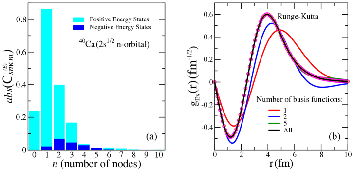
Figure 1: (a) Absolute value of the projections (or amplitudes) of the $2s^{\frac{1}{2}}$ ($\kappa\!=\!-1$) neutron orbital in ${}^{40}\text{Ca}$ on to the various Dirac oscillator basis states; see Eq.(22). The horizontal axis denotes the number of nodes in the first 11 $\kappa\!=\!-1$ basis states. The light (dark) blue bars represent the contribution from the positive (negative) energy states. (b) Piecewise reconstruction of the upper component of $2s^{\frac{1}{2}}$ ($\kappa\!=\!-1$) neutron orbital in ${}^{40}\text{Ca}$ by combining the various Dirac oscillator basis states in order of importance. For example, the red line includes the most important basis state (i.e., the $n\!=\!1$ positive energy state). In turn, the blue line includes the two most important states and so on. The black line includes the contribution of all basis states used in the diagonalization procedure. Finally, the curve depicted with the magenta circles was obtained from using the Runge-Kutta algorithm.

The main purpose of this section is to test the reliability of the Dirac oscillator basis and to discuss the new insights that emerge from such an approach. Although we start with scalar and vector potentials that are spherically symmetric, we will discuss how to construct the Hamiltonian matrix for the more general case of an axially-symmetric problem where the $z$-component of the angular momentum $m$ remains the only good quantum number. One starts by dividing the Hamiltonian matrix $H_{\rm DFT}$ into blocks, each with a well defined value of $m$. For a given value of $m$, the minimum value of the total angular momentum is given by $j_{\rm min}\!=\!|m|$, which in turn implies a minimum value of $|\kappa_{\rm min}|\!=\!j_{\rm min}\!+\!1/2\!=\!|m|+1/2$. The maximum value of $\kappa$ is set by the single-particle orbital with the largest value of the total angular momentum. Given that in this paper we focus on the four doubly-magic nuclei ${}^{40}\text{Ca}$, ${}^{48}\rm{Ca}$, ${}^{132}\rm{Sn}$, and ${}^{208}\rm{Pb}$, the occupied single-particle orbital with the largest value of the total angular momentum is the $i^{13/2}$ ($\kappa\!=\!-7$) neutron orbital in ${}^{208}\rm{Pb}$. Hence, we set $|\kappa_{\rm max}|\!=\!10$, a value that was found to yield well-converged results. Regardless of whether the problem involves spherical symmetry or not, one must also specify the maximum value of $n$. As one increases the number of nodes $n$, one can account for higher momentum components in the wave function. Although for the most extreme case of ${}^{208}\rm{Pb}$ no single-particle orbital displays more than two nodes, we selected $n_{\rm max}\!=\!10$. The results improve very rapidly with increasing $n_{\rm max}$ and are fully converged by $n_{\rm max}\!=\!10$. Note that the range of values adopted for $n$ and $\kappa$ are used for both the positive- and negative-energy sector. Also note that if the entire Hamiltonian is spherically symmetric, one “discovers” that states with different values of $\kappa$ do not mix.

Having identified the Dirac oscillator states that will be used to build the Hamiltonian matrix, one must select the value of the oscillator frequency $\omega$, or equivalently the oscillator length parameter $b\!\equiv\!1/\!\sqrt{m\omega}$. Although in principle one could optimize the diagonalization by selecting the parameter variationally, for our purposes it was sufficient to fix $b$ by demanding good agreement with the lowest $s^{1/2}$ proton orbital in ${}^{208}\rm{Pb}$. By doing so, the value of the oscillator parameter was fixed to $b\!=\!2.4\,{\rm fm}$. Although an optimal value of $b$ reduces the number of basis states required to reproduce the entire spectrum, the adopted value of $b$—together with the range of values chosen for $n$ and $\kappa$—produced stable results for all nuclei under consideration. Finally, to test the reliability of the method we selected the FSUGold model introduced in Ref. Todd-Rutel and Piekarewicz (2005).

Predictions for the binding energy per nucleon and the neutron skin thickness of the doubly-magic nuclei ${}^{40}\text{Ca}$, ${}^{48}\rm{Ca}$, ${}^{132}\rm{Sn}$, and ${}^{208}\rm{Pb}$ are displayed in Table. 1 using both the Runge-Kutta algorithm as well as the Dirac oscillator basis. The neutron skin thickness, a sensitive isovector observable, is defined as the difference between the neutron and proton root-mean-square radii. Evidently, the agreement between the two methods is excellent—even when the small neutron skin thickness emerges from the difference of two radii of similar size.

Besides the fact that the Dirac oscillator method can be easily generalized to the study of axially-deformed nuclei, the method also provides valuable insights. For example, how are the eigenstates of $\hat{H}_{\rm DFT}$ expressed as a linear combination of the Dirac oscillator states? To answer this question we select the $2s^{1/2}$ neutron orbital in ${}^{40}\text{Ca}$ as an example; that is, the orbital with one interior node. In this case spherical symmetry is still preserved so $\kappa\!=\!-1$ emerges as a good quantum number. The corresponding eigenstate may be expressed in terms of the Dirac oscillator basis as follows:

$$|\psi_{E\kappa m}\rangle=\sum_{sn}C_{sn\kappa m}^{(E)}|sn\kappa m\rangle,$$ (22)

where the associated amplitudes $C_{sn\kappa m}^{(E)}$ that emerge from the diagonalization procedure satisfy the normalization condition

$$\sum_{sn}\left|C_{sn\kappa m}^{(E)}\right|^{2}=1.$$ (23)

We display on the left-hand panel of Fig. 1 the absolute value of the amplitudes $C_{sn\kappa m}^{(E)}$ for the $2s^{1/2}$ neutron orbital in ${}^{40}\text{Ca}$ as a function of the number of nodes of each individual basis state $|s,n,\kappa\!=\!-1,m\!=\!0\rangle$. However, since the positive energy states by themselves do not form a complete basis, we depict with the light-blue bars the projections (or amplitudes) into the positive energy states and with dark-blue bars the corresponding projections into the negative energy states. As expected, the largest amplitude is carried by the positive energy state having one interior node. The contribution from this one basis state to the entire upper component of the wave function may be seen on the right-hand panel of Fig. 1. The $n\!=\!2,0,3$ are the next most important basis states, respectively. Yet, the next most important contribution after that comes from the $n\!=\!2$ negative energy state. Indeed, with only 5 basis states one can accurately capture the shape of the exact wave function; see Fig. 1(b). Although small, the contribution from the negative energy sector is vital to accurately reproduce the entire wave function, which is displayed with the black solid line (labeled “All”) in Fig. 1(b). The curve depicted with the red circles represents the exact solution obtained using the Runge-Kutta method and it is clearly indistinguishable from the black line. This simple, yet illustrative example, confirms that the Dirac oscillator basis is both efficient and insightful for the solution of relativistic nuclear-structure problems.

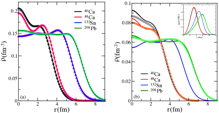
Figure 2: (a) Baryon (neutron-plus-proton) densities of ${}^{40}\text{Ca}$, ${}^{48}\rm{Ca}$, ${}^{132}\rm{Sn}$, and ${}^{208}\rm{Pb}$ as predicted by the FSUGold model Todd-Rutel and Piekarewicz (2005). Results from the Dirac oscillator method are denoted with the solid lines whereas those obtained from the Runge-Kutta algorithm are depicted with the various symbols. (b) Same as in panel (a) but now for the charge density. The nearly identical predictions from the Dirac oscillator and Runge-Kutta methods are plotted jointly as solid lines whereas the experimental results De Vries et al. (1987) are depicted with the various symbols. Note that at present there is no measurement of the charge distribution of ${}^{132}\rm{Sn}$, although see Suda et al. (2009); Tsukada et al. (2017). Finally, the inset displays the charge density multiplied by a suitable phase-space factor that makes the integral under the curve identically equal to one for all nuclei.

We close this section by displaying in Fig. 2 the baryon (neutron-plus-proton) density as well as the charge density as predicted by the FSUGold model Todd-Rutel and Piekarewicz (2005) for ${}^{40}\text{Ca}$, ${}^{48}\rm{Ca}$, ${}^{132}\rm{Sn}$, and ${}^{208}\rm{Pb}$. On the left-hand panel we highlight the excellent agreement between the Runge-Kutta and Dirac oscillator methods in predicting the baryon density—a ground-state property that is sensitive to all nucleon orbitals. Given the excellent agreement between the two methods, we display in Fig. 2(b) their predictions (combined in a single solid line) alongside the experimental charge density (depicted with symbols) for ${}^{40}\text{Ca}$, ${}^{48}\rm{Ca}$, and ${}^{208}\rm{Pb}$ De Vries et al. (1987). Note that at present the charge density of ${}^{132}\rm{Sn}$ is unknown, although enormous progress is being made in the development of electron-scattering techniques for the measurement of the charge density of short-lived isotopes Suda et al. (2009); Tsukada et al. (2017). Although the charge radius of several closed-shell nuclei was used in the calibration of the FSUGold functional, a common deficiency of models of this kind is the poor reproduction of the interior density, a behavior that is controlled by the high-momentum components of the charge form factor. Perhaps a more reliable comparison between theory and experiment is the phase-space weighted charge density displayed in the inset of Fig. 2(b) and defined as,

$$\widetilde{\rho}(r)\equiv\frac{1}{Z}4\pi r^{2}\rho(r)\hskip 10.0pt{\rm with}\hskip 10.0pt\int_{0}^{\infty}\widetilde{\rho}(r)dr=1.$$ (24)

In particular, $\widetilde{\rho}(r)$ has been normalized to 1 for all nuclei and its second moment equals the mean-square radius of the charge distribution.

IV Conclusion

The staple of nuclear structure is the nuclear shell model, a theoretical framework that in its simplest form consists of a harmonic oscillator model supplemented by a strong spin-orbit interaction Haxel et al. (1949); Mayer (1949). Although more than seven decades have passed since its original formulation, this simplest version of the nuclear shell model continues to be used today—often as the first step in the development of more sophisticated models. Initially modeled after the Thomas term in atomic systems, it was soon realized that: “There is no adequate theoretical reason for the large observed value of the spin orbit coupling ” Mayer (1950). Ultimately, of course, the complex dynamical origin of the nuclear spin-orbit force hides within QCD. Nevertheless, inspired by Yukawa’s meson theory, early attempts at building a relativistic models of the nuclear force considered nucleons interacting by the exchange of isoscalar meson fields of Lorentz scalar and vector character Johnson and Teller (1955); Duerr (1956); Miller and Green (1972); Walecka (1974). While successful in many regards Serot and Walecka (1986), the models also provided a natural explanation for the emergence of a strong spin-orbit force. Since then, relativistic nuclear models have been augmented and refined—and are now part of a vast arsenal of theoretical tools devoted to the study of diverse nuclear phenomena. It is in this overall context that we find surprising that the Dirac oscillator model of Moshinsky and Szczepaniak Moshinsky and Szczepaniak (1989)—which may be cast in the form of an ordinary oscillator model with a strong spin-orbit term—has remained largely unknown to the nuclear physics community. The present contribution aims to remedy this situation.

In this paper we introduced the Dirac oscillator and highlighted some of its remarkable properties. Mainly, the fact that the Dirac oscillator can be solved exactly given that both of its upper and lower components satisfy Schrödinger-like equations identical to the conventional harmonic oscillator supplemented by a strong spin-orbit interaction. Matrix elements of a mean-field Hamiltonian containing strong scalar and (time-like) vector potentials were computed in the Dirac oscillator basis. Once the matrix elements were obtained, we carried out the entire self-consistent procedure, which involved solving Klein-Gordon equations for the meson fields and diagonalizing the mean-field Hamiltonian for the nucleon field until convergence was achieved. By selecting a reasonable value for the oscillator frequency, or equivalent the oscillator length, relatively modest-size matrices had to be diagonalized. We note that while the contribution from the negative energy sector of the Dirac oscillator played a relatively minor role, it was by no means negligible. Finally, we compared results against those obtained using the Runge-Kutta method. In all instances the comparisons between the two methods were excellent. Yet, we argue that relative to the Runge-Kutta method, the Dirac oscillator method has the distinct advantage that the generalization to problems with broken spherical symmetry is fairly straightforward.

Problems with axial symmetry may play a pivotal role in the refinement of modern energy density functionals. The standard fitting protocol of energy density functionals (both covariant and non-relativistic) involves calibrating the parameters of the model by invoking genuine physical observables—mostly ground-state properties such as binding energies and charge radii. However, these observables are insensitive to certain critical aspects of the nuclear dynamics. For example, whereas binding energies and charge radii effectively constrain the saturation point (density and binding energy per nucleon) of symmetric nuclear matter, they provide little guidance on the incompressibility coefficient. In an effort to remedy this deficiency, experimental information on isoscalar giant monopole energies—which are strongly correlated to the incompressibility coefficient—are now incorporated into the calibration of the functionals Chen and Piekarewicz (2014). However, in an effort to reduce the computational demands, giant-monopole energies were computed in a constrained approach, thereby avoiding the need for computationally demanding random-phase-approximation (RPA) calculations Chen et al. (2013). In a constrained approach, giant-monopole energies may be directly computed from a ground-state calculation by adding to the Hamiltonian a “constrained” one-body term proportional to the operator responsible for the excitation, namely, $\lambda r^{2}$. Note that for monopole excitations the Hamiltonian remains spherically symmetric.

Whereas binding energies, charge radii, and giant-monopole energies provide stringent constraints on the isoscalar sector of the functional, the lack of experimental data on exotic nuclei with a large neutron-proton asymmetries has hindered our knowledge of the isovector sector. It has been recognized that the neutron skin thickness of neutron rich nuclei such as ²⁰⁸Pb and ⁴⁸Ca can effectively constrain the isovector sector, particularly the density dependence of the nuclear symmetry energy, and experimental campaigns are currently underway at JLab to determine the thickness of the neutron skin in a clean and largely model independent way Abrahamyan et al. (2012); Horowitz et al. (2012); CRE . The electric dipole polarizability has also been shown to be a strong isovector indicator Reinhard and Nazarewicz (2010); Piekarewicz et al. (2012); Roca-Maza et al. (2013). The electric dipole polarizability is a static observable that is proportional to the inverse energy weighted sum $m_{-1}$ of the isovector dipole response. As such, $m_{-1}$ may be computed from a ground-state calculation by adding a “constrained” one-body term of the form: $\lambda rY_{1,0}(\theta,\varphi)\tau_{z}$. As already shown here, matrix elements of operators of the general form $r^{L}Y_{L,0}(\theta,\varphi)$ may be readily evaluated in the Dirac oscillator basis. Hence, in principle one may incorporate experimental information on the electric dipole polarizability in the calibration of the functional, by either computing $m_{-1}$ in a constrained approach or by computing the entire isovector dipole response in a relativistic random phase approximation. Although successful in computing various moments of the monopole and quadrupole distribution in a constrained approach, so far we have been unable to obtain stable results for the electric dipole polarizability. To date, the only successful approach that we are aware of is the one by Yuksel, Marketin, and Paar Yuksel et al. (2019), in which the calibration of a new “point coupling” model involved computing the entire isovector dipole response.

In summary, we have demonstrated that the Dirac oscillator basis provides an ideal tool for solving nuclear-structure problems formulated within the framework of covariant density functional theory. Indeed, excellent agreement was obtained when compared against results generated using the Runge-Kutta method. The Dirac oscillator incorporates two features that have been at the core of nuclear structure since its inception: (i) a harmonic oscillator basis supplemented by (ii) a strong spin-orbit coupling. In this paper we outlined the steps that are necessary to compute matrix elements of an axially symmetric relativistic mean-field Hamiltonian in the Dirac oscillator basis. Problems of this kind are useful for understanding the structure of deformed nuclei as well as in computing various moments of the nuclear response in a constrained approach. Ultimately, an efficient and robust computation of these moments could significantly improve the quality of future covariant energy density functionals.

V Appendix

In this section we provide a detailed derivation of the energies and corresponding eigenfunctions of the relativistic Dirac oscillator. Given the spherical symmetry of the potential, we start by writing the 4-component solution as follows Sakurai (1967):

$$\psi_{E\kappa m}(\bm{r})\!=\!\left(\begin{array}[]{c}\phi_{E\kappa m}(\bm{r})\\ \chi_{E\kappa m}(\bm{r})\end{array}\right)\!=\!\left(\begin{array}[]{c}\phantom{i}g_{E\kappa}(r)\left|+\kappa m\right\rangle\\ if_{E\kappa}(r)\left|-\kappa m\right\rangle\end{array}\right),$$ (A.1)

where both $g_{E\kappa}(r)$ and $f_{E\kappa}(r)$ are real functions of $r$ and the spin-spherical harmonics $|\kappa m\rangle$ have been defined in Eq. (7). As shown in Eq. (10), the upper component of the Dirac equation satisfies a Schrödinger-like equation supplemented by a strong spin-orbit term:

$$\left(\frac{\bm{p}^{2}}{2m}\!+\!\frac{1}{2}m\omega^{2}\bm{r}^{2}\!-\!\omega\bm{\sigma}\cdot\bm{L}\right)\!\phi(\bm{r})\!=\!\left(\frac{E^{2}\!-\!m^{2}\!+\!3m\omega}{2m}\right)\!\phi(\bm{r}).$$ (A.2)

Because of the appearance of the spin-orbit interaction, the energies of the Dirac oscillator depend strongly on the generalized angular momentum quantum number $\kappa$. That is,

$$\frac{E^{2}-m^{2}}{2m}=\begin{cases}\ 2n\omega&\text{if }\kappa<0,\\ \left(2n+2l+1\right)\omega&\text{if }\kappa>0.\end{cases}$$ (A.3)

In particular, for $\kappa\!<\!0$ the energies are independent of any angular momentum quantum number (i.e., $l$ and $j$) so the spectrum—for a fixed value of $n$—displays an infinite degeneracy. Although more reminiscent of the ordinary oscillator, the energies for $\kappa\!>\!0$ weigh equally the number of nodes $n$ as the orbital angular momentum quantum number $l$; recall that in the ordinary case nodes cost twice as much energy as $l$.

At this point it is useful to invoke some well known results from the ordinary harmonic oscillator. For example, the radial solution of the isotropic, three dimensional harmonic oscillator is

$$R_{nl}(x)=A_{nl}\,x^{l}{\cal M}\!\left(-n,l\!+\!\frac{3}{2},x^{2}\right){{e}}^{-x^{2}/2},$$ (A.4)

where $n$ is the number of interior nodes, $l$ is the orbital angular momentum, $x\!\equiv\!r/b$ is the dimensionless radial distance measured in units of the oscillator-length parameter $b\!=\!1/\sqrt{m\omega}$, and $A_{nl}$ is the normalization constant given by

$$A_{nl}=\sqrt{\frac{2\,\Gamma(n\!+\!l\!+\!3/2)}{(n!)\,\Gamma^{2}(l\!+\!3/2)}}.$$ (A.5)

Besides the characteristic Gaussian falloff, the radial dependence of $R_{nl}(r)$ is contained in Kummer’s function Abramowitz and Stegun :

$${\cal M}(\alpha,\beta,z)=\sum_{m=0}^{\infty}\frac{(\alpha)_{m}}{(\beta)_{m}}\frac{z^{m}}{m!}\,,$$ (A.6a)

$${\rm with}\hskip 5.0pt (\alpha)_{m}\equiv\alpha(\alpha+1)(\alpha+2)\ldots(\alpha+m-1).$$ (A.6b)

Although in principle the above sum extends up to infinity, in practice the sum is truncated after $n\!+\!1$ terms, making ${\cal M}(-n,\alpha,\beta)$ a polynomial of degree $n$; note that $(\alpha)_{0}\!\equiv\!1$. In this way, we can write the upper component of the radial solution of the Dirac equation simply as

$$g_{E\kappa}(r)=R_{nl}(x\!=\!r/b),$$ (A.7)

where the energy is given in Eq. (A.3) and $\kappa$ is related to $l$ via Eq. (7). Having solved for the upper component, the lower component may be obtained by differentiation. That is, using Eq. (9a) one obtains

$$\chi(\bm{r})=\frac{(\bm{\sigma}\cdot\bm{\pi}_{-})}{(E+m)}\phi(\bm{r})=\frac{\bm{\sigma}\cdot\left({\bf p}-im\omega{\bf r}\right)}{(E+m)}\phi(\bm{r})$$

$$=\frac{i}{(E\!+\!m)}\left[\frac{\partial}{\partial r}\!+\!\frac{(\kappa\!+\!1)}{r}\!+\!m\omega r\right]\!g_{E\kappa}(r)\left|-\kappa m\rangle\right..$$ (A.8)

Comparing this expression to Eq.(A.1) we conclude that

$$f_{E\kappa}(r)= \left(\frac{1}{E+m}\right)\left[\frac{d}{dr}\!+\!\frac{(\kappa\!+\!1)}{r}\!+\!m\omega r\right]g_{E\kappa}(r)$$

$$= \left(\frac{b^{-1}}{E+m}\right)\left[\frac{d}{dx}\!+\!\frac{(\kappa\!+\!1)}{x}\!+\!x\right]R_{nl}(x).$$ (A.9)

Now, by direct differentiation of Eq. (A.4) one obtains

$$\left[\frac{d}{dx}\!+\!\frac{(\kappa\!+\!1)}{x}\!+\!x\right]R_{nl}(x)=$$

$$A_{nl}\,x^{l} \left[2xM^{\prime}(\alpha,\beta,x^{2})\!+\!\frac{(l\!+\!\kappa\!+\!1)}{x}M(\alpha,\beta,x^{2})\right]{{e}}^{-x^{2}/2},$$ (A.10)

where $\alpha\!=\!-n$, $\beta\!=\!l+3/2$, and the “prime” indicates differentiation with respect to the argument (i.e., $x^{2}$). At this point one must distinguish between $\kappa\!<\!0$ and $\kappa\!>\!0$ and for this we use the following two useful relations involving Kummer’s functions Abramowitz and Stegun :

$$\frac{dM(\alpha,\beta,z)}{dz} \!=\!\frac{\alpha}{\beta}M(\alpha\!+\!1,\beta\!+\!1,z),$$ (A.11a)

$$z\frac{dM(\alpha,\beta,z)}{dz} \!=\!(\beta\!-\!1)\left[M(\alpha,\beta\!-\!1,z)\!-\!M(\alpha,\beta,z)\right],$$ (A.11b)

where the first identity is used for $\kappa\!<\!0$ and the second one for $\kappa\!>\!0$. Using these relations one obtains simple and illuminating expressions for the lower component of the Dirac oscillator

$$f_{E\kappa}(r) =\left(\frac{b^{-1}}{E+m}\right)\left[\frac{d}{dx}\!+\!\frac{(\kappa\!+\!1)}{x}\!+\!x\right]R_{nl}(x)$$

$$=\zeta_{\kappa}\frac{\sqrt{E^{2}-m^{2}}}{E+m}\,R_{n^{\prime}l^{\prime}}(x),$$ (A.12)

where $\zeta_{\kappa}\!=\!{\rm sgn}(\kappa)$, and $n^{\prime}$ and $l^{\prime}$ are defined as

$$n^{\prime}=\begin{cases}n&\text{if }\kappa>0,\\ n\!-\!1&\text{if }\kappa<0,\end{cases}\quad l^{\prime}=\begin{cases}l\!-\!1&\text{if }\kappa>0,\\ l\!+\!1&\text{if }\kappa<0.\end{cases}$$ (A.13)

This illustrates the well known fact that the upper and lower components of the Dirac wave function have different intrinsic parities, namely, $l^{\prime}\!=\!l\!\pm\!1$. That is, in the relativistic framework the orbital angular momentum is no longer a good quantum number.

We can now proceed to write the properly normalized eigenstates of the Dirac oscillator. For the positive energy ($E\!>\!0$) sector one obtains

$$\psi_{E\kappa m}(\bm{r})\!=\!\left(\begin{array}[]{l}\phantom{+i\zeta_{\kappa}}\displaystyle{\sqrt{\frac{E\!+\!m}{2E}}\,R_{nl}(r)}\left|+\kappa m\right\rangle\vspace{5pt}\\ +i\zeta_{\kappa}\,\displaystyle{\sqrt{\frac{E\!-\!m}{2E}}\,R_{n^{\prime}l^{\prime}}(r)}\!\left|-\kappa m\right\rangle\end{array}\right).$$ (A.14)

In turn, eigenstates of the Dirac oscillator with negative energy ($E\!<\!0$) are given by

$$\psi_{E\kappa m}(\bm{r})\!=\!\left(\begin{array}[]{l}\phantom{-i\zeta_{\kappa}}\displaystyle{\sqrt{\frac{|E|\!-\!m}{2|E|}}\,R_{nl}(r)}\left|+\kappa m\right\rangle\vspace{5pt}\\ -i\zeta_{\kappa}\,\displaystyle{\sqrt{\frac{|E|\!+\!m}{2|E|}}\,R_{n^{\prime}l^{\prime}}(r)}\!\left|-\kappa m\right\rangle\end{array}\right).$$ (A.15)

Such a simple expression is reminiscent of the plane-wave (i.e., free) solutions of the Dirac equation, which for positive energy are

$$g_{E\kappa}(r) =j_{l}(kr),$$ (A.16a)

$$f_{E\kappa}(r) =\pm\sqrt{\frac{E-m}{E+m}}\,j_{l^{\prime}}(kr),$$ (A.16b)

where $k\!=\!\sqrt{E^{2}\!-\!m^{2}}$, and $j_{l}(x)$ are $j_{l^{\prime}}(x)$ are spherical Bessel functions. The remarkable feature of Eq. (A.15) is that such a compact expression emerges even in the case of the highly non-trivial Dirac oscillator.

References

- Haxel et al. (1949) O. Haxel, J. H. Jensen, and H. Suess, Phys. Rev. 75, 1766 (1949).
- Mayer (1949) M. G. Mayer, Phys. Rev. 75, 1969 (1949).
- (3) M. G. Mayer, “The Shell Model: 1963 Nobel Lecture,” https://www.nobelprize.org/uploads/2018/06/mayer-lecture.pdf.
- Brown (2001) B. A. Brown, Prog. Part. Nucl. Phys. 47, 517 (2001).
- Dickhoff and Barbieri (2004) W. H. Dickhoff and C. Barbieri, Prog. Part. Nucl. Phys. 52, 377 (2004).
- Roth et al. (2010) R. Roth, T. Neff, and H. Feldmeier, Prog. Part. Nucl. Phys. 65, 50 (2010).
- Kortelainen et al. (2010) M. Kortelainen, T. Lesinski, J. More, W. Nazarewicz, J. Sarich, et al., Phys. Rev. C82, 024313 (2010).
- Hagen et al. (2014) G. Hagen, T. Papenbrock, M. Hjorth-Jensen, and D. J. Dean, Rept. Prog. Phys. 77, 096302 (2014).
- Barrett et al. (2013) B. R. Barrett, P. Navratil, and J. P. Vary, Prog. Part. Nucl. Phys. 69, 131 (2013).
- Serot and Walecka (1986) B. D. Serot and J. D. Walecka, Adv. Nucl. Phys. 16, 1 (1986).
- Meng (2016) J. Meng, “Relativistic density functional for nuclear structure,” (World Scientific, New Jersey, 2016).
- Chen and Piekarewicz (2014) W.-C. Chen and J. Piekarewicz, Phys. Rev. C90, 044305 (2014).
- Horowitz and Serot (1981) C. J. Horowitz and B. D. Serot, Nucl. Phys. A368, 503 (1981).
- Todd and Piekarewicz (2003) B. G. Todd and J. Piekarewicz, Phys. Rev. C67, 044317 (2003).
- Vretenar et al. (2005) D. Vretenar, A. Afanasjev, G. Lalazissis, and P. Ring, Phys. Rept. 409, 101 (2005).
- Moshinsky and Szczepaniak (1989) M. Moshinsky and A. Szczepaniak, J. Phys. A: Math Gen. 22, L817 (1989).
- Itô et al. (1967) D. Itô, K. Mori, and E. Carriere, Nuovo Cimento A 51, 1119 (1967).
- Quesne and Moshinsky (1990) C. Quesne and M. Moshinsky, J. Phys. A: Math Gen. 23, 2263 (1990).
- Johnson and Teller (1955) M. H. Johnson and E. Teller, Phys. Rev. 98, 783 (1955).
- Duerr (1956) H.-P. Duerr, Phys. Rev. 103, 469 (1956).
- Miller and Green (1972) L. D. Miller and A. E. S. Green, Phys. Rev. C5, 241 (1972).
- Walecka (1974) J. D. Walecka, Annals Phys. 83, 491 (1974).
- Boguta and Bodmer (1977) J. Boguta and A. R. Bodmer, Nucl. Phys. A292, 413 (1977).
- Mueller and Serot (1996) H. Mueller and B. D. Serot, Nucl. Phys. A606, 508 (1996).
- Lalazissis et al. (1997) G. A. Lalazissis, J. Konig, and P. Ring, Phys. Rev. C55, 540 (1997).
- Lalazissis et al. (2005) G. A. Lalazissis, T. Niksic, D. Vretenar, and P. Ring, Phys. Rev. C71, 024312 (2005).
- Todd-Rutel and Piekarewicz (2005) B. G. Todd-Rutel and J. Piekarewicz, Phys. Rev. Lett 95, 122501 (2005).
- Chen and Piekarewicz (2015) W.-C. Chen and J. Piekarewicz, Phys. Lett. B748, 284 (2015).
- (29) J. Yang and J. Piekarewicz, arXiv:1912.11112 [nucl-th] .
- Stoitsov et al. (1998) M. Stoitsov, P. Ring, D. Vretenar, and G. Lalazissis, Physical Review C 58, 2086 (1998).
- Li et al. (2012) L. Li, J. Meng, P. Ring, E.-G. Zhao, S.-G. Zhou, et al., Physical Review C 85, 024312 (2012).
- Martinez-Romero et al. (1995) R. P. Martinez-Romero, H. N. Nuñez-Yépez, and A. L. Salas-Brito, European Journal of Physics 16, 135 (1995).
- Sakurai (1967) J. J. Sakurai, “Advanced quantum mechanics,” (Pearson Education, 1967).
- De Vries et al. (1987) H. De Vries, C. W. De Jager, and C. De Vries, Atom. Data Nucl. Data Tabl. 36, 495 (1987).
- Suda et al. (2009) T. Suda et al., Phys. Rev. Lett. 102, 102501 (2009).
- Tsukada et al. (2017) K. Tsukada et al., Phys. Rev. Lett. 118, 262501 (2017).
- Mayer (1950) M. G. Mayer, Phys. Rev. 78, 16 (1950).
- Yuksel et al. (2019) E. Yuksel, T. Marketin, and N. Paar, Phys. Rev. C99, 034318 (2019).
- Chen et al. (2013) W.-C. Chen, J. Piekarewicz, and M. Centelles, Phys. Rev. C 88, 024319 (2013).
- Abrahamyan et al. (2012) S. Abrahamyan, Z. Ahmed, H. Albataineh, K. Aniol, D. S. Armstrong, et al., Phys. Rev. Lett. 108, 112502 (2012).
- Horowitz et al. (2012) C. J. Horowitz, Z. Ahmed, C. M. Jen, A. Rakhman, P. A. Souder, et al., Phys. Rev. C85, 032501 (2012).
- (42) “CREX: Parity-violating measurement of the weak charge distribution of 48Ca,” http://hallaweb.jlab.org/parity/prex/c-rex/c-rex.pdf.
- Reinhard and Nazarewicz (2010) P.-G. Reinhard and W. Nazarewicz, Phys. Rev. C81, 051303 (2010).
- Piekarewicz et al. (2012) J. Piekarewicz, B. Agrawal, G. Colò, W. Nazarewicz, N. Paar, et al., Phys. Rev. C85, 041302(R) (2012).
- Roca-Maza et al. (2013) X. Roca-Maza, M. Centelles, X. Viñas, M. Brenna, G. Colò, et al., Phys. Rev. C88, 024316 (2013).
- (46) M. Abramowitz and Stegun, “Handbook of mathematical functions with formulas” .