Continuation of relative equilibria in the $n$–body problem to spaces of constant curvature

Abstract

We prove that all non-degenerate relative equilibria of the planar Newtonian $n$–body problem can be continued to spaces of constant curvature $\kappa$, positive or negative, for small enough values of this parameter. We also compute the extension of some classical relative equlibria to curved spaces using numerical continuation. In particular, we extend Lagrange’s triangle configuration with different masses to both positive and negative curvature spaces.

Keywords: relative equilibria, spaces of constant curvature, curved $n$–body problem, Palais slice coordinates.

Subjclass[2020] 70F10, 70F07, 70F15, 34A25

1 Introduction

The curved $n$–body problem is a natural extension of the planar Newtonian $n$–body problem to surfaces of nonzero constant curvature. The origin of this problem is in the Kepler and the two body problem on curved spaces, first studied independently by Lobachevsky and Bolyai (co-discoverers of the first non-Euclidean geometries), in the 1830’s. Since then, many authors have worked on this problem, developed their original geometric ideas and expressed them in analytical and modern language; among others, E. Shering, H. Liebmann, P. Serré, and many names from the Russian school (see [7] and [2] for a nice historical review on this problem).

In [9], the Kepler and the two–body problem was extended to the curved $n$–body problem on spaces of positive and negative curvature in an unified way. In this paper the authors show that the Lagrangian equilateral triangle solutions exist on spaces of constant curvature if and only if the three masses are equal. Since then, a natural and pressing question emerged: Is it possible to extend any type of planar Newtonian relative equilibrium (curvature $\kappa=0$) to surfaces of constant curvature different from zero? In particular, what happens with the Lagrangian solutions of the Newtonian problem when all masses are not equal? Can they be continued to curved surfaces?

Most researchers in the field though that this conjecture should be true, but it has remained an open problem until today. In this paper we finally present two proofs of this conjecture and a numerical continuation procedure to compute relative equilibria for negative and positive curvature.

In recent years, relative equilibria on curved spaces have received considerable attention; we now mention some related works. For the case of $n=3$ equal masses, the authors in [4] perform an extensive analysis of the stability of the Lagrangian relative equilibria on spaces of positive curvature, showing all possible bifurcation values and the regions on the sphere where they are stable. More generally, they study the homographic orbits generated by this kind of relative equilibria. In [5] the same authors study relative equilibria of the restricted three-body problem, when the two primary masses form a relative equilibrium. For the case of $n=2$ masses, the authors in [3] perform an interesting analysis of the relative equilibria on spaces of constant curvature using reduction and techniques from geometric mechanics, and rediscover some results stated and proved first in [14], but with simpler proofs. In [17] the authors show an inverse result for the collinear curved $5$ and $7$ problem, where collinear means that all masses are located on the same geodesic for all time. The same authors in [18] show a local and general regularization result for the restricted $n$–body problem, when the $n$ primary equal masses form a relative equilibria.

Notice that all these previous works deal with particular cases, while our present result applies to any non-degenerate relative equilibria (arbitrary number of bodies, unequal masses, etc.). On the other hand, our result is perturbative and applies only for small enough curvature.

The paper is organized as follows: In Section 2, starting from a unified model for the curved $n$–body problem, we express the corresponding Lagrangian in rotating coordinates and obtain the kinetic and potential energy as an expansion in terms of the curvature $\kappa$. In Section 3 we prove the continuation of relative equilibria to spaces of constant curvature using Palais slice coordinates. In Section 4 we give an alternative proof using Lagrange multipliers that is better suited for computations. Finally in Section 5 we implement the continuation numerically and show several examples, both for positive and negative curvatures.

2 Unified model for the $n$–body problem in spaces of constant curvature

In this section we write the Lagrangian for the curved $n$–body problem for positive and negative curvature $\kappa$, and we show that it can be written in a unified way for all $\kappa$ (positive, negative, and zero).

2.1 Lagrangian of $n$ bodies on the sphere of positive curvature $\kappa$

From [16], the Lagrangian for $n$ bodies in the sphere of radius $R$, where the position of the body with mass $m_{j}$ is parametrized by the stereographic projection $z_{j}\in\mathbb{C}$, is given by

$$L(z,\dot{z};R)=T(z,\dot{z})+U(z),$$ (1)

where the kinetic and potential energies are

$$T=\frac{1}{2}\sum_{j=1}^{n}m_{j}\lambda(z_{j})\left|\dot{z}_{j}\right|^{2},\qquad U=\sum_{j<k}m_{k}m_{j}V(z_{j},z_{k})\text{.}$$ (2)

The function $\lambda$ is the conformal factor coming from the stereographic projection through the north pole of the sphere into the plane of the ecuator, and the potential $V$ corresponds to the mutual attraction among the particles. Both functions are analytic in $z_{j}$ and $\bar{z}_{j}$ (i.e. analytic as a function of the real coordinates $x_{j}$ and $y_{j}$) and given by

$$V(z_{j},z_{k}) =\frac{1}{R}\frac{\frac{4\operatorname{Re}\left(z_{j}\bar{z}_{k}\right)}{R^{2}}+\left(\frac{\left|z_{k}\right|^{2}}{R^{2}}-1\right)\left(\frac{\left|z_{j}\right|^{2}}{R^{2}}-1\right)}{\sqrt{\left(\frac{\left|z_{k}\right|^{2}}{R^{2}}+1\right)^{2}\left(\frac{\left|z_{j}\right|^{2}}{R^{2}}+1\right)^{2}-\left(\frac{4\operatorname{Re}\left(z_{j}\bar{z}_{k}\right)}{R^{2}}+\left(\frac{\left|z_{k}\right|^{2}}{R^{2}}-1\right)\left(\frac{\left|z_{j}\right|^{2}}{R^{2}}-1\right)\right)^{2}}},$$

$$\lambda(z_{j}) =\frac{4}{\left(1+\frac{\left|z_{j}\right|^{2}}{R^{2}}\right)^{2}}\text{.}$$

The positive curvature $\kappa$ depends on the radius $R$ as

$$\kappa=\frac{1}{R^{2}}\text{.}$$

Thus the functions $V$ and $\lambda$ expressed in terms of the curvature are

$$V(z_{j},z_{k}) =\frac{4\operatorname{Re}\left(z_{j}\bar{z}_{k}\right)\kappa+\left(\left|z_{k}\right|^{2}\kappa-1\right)\left(\left|z_{j}\right|^{2}\kappa-1\right)}{\sqrt{\kappa^{-1}\left(\left|z_{k}\right|^{2}\kappa+1\right)^{2}\left(\left|z_{j}\right|^{2}\kappa+1\right)^{2}-\kappa^{-1}\left(4\operatorname{Re}\left(z_{j}\bar{z}_{k}\right)\kappa+\left(\left|z_{k}\right|^{2}\kappa-1\right)\left(\left|z_{j}\right|^{2}\kappa-1\right)\right)^{2}}},$$ (3)

$$\lambda(z_{j}) =\frac{4}{\left(1+\kappa\left|z_{j}\right|^{2}\right)^{2}}\text{.}$$ (4)

2.2 Lagrangian of $n$ bodies on the hyperbolic sphere of negative curvature $\kappa<0$.

From [8], the Lagrangian for $n$ bodies in the hyperbolic sphere of radius $R$, where the position of the body with mass $m_{j}$ is parametrized by the stereographic projection $z_{j}\in\mathbb{C}$, is given by

$$L(z,\dot{z};R)=T(z,\dot{z})+U(z),$$ (5)

where the kinetic and potential energies are defined by (2) with the functions $\lambda$ and $V$ given by

$$V(z_{j},z_{k}) =\frac{\frac{-4\operatorname{Re}\left(z_{j}\bar{z}_{k}\right)}{R^{2}}+\left(-\frac{\left|z_{k}\right|^{2}}{R^{2}}-1\right)\left(-\frac{\left|z_{j}\right|^{2}}{R^{2}}-1\right)}{\sqrt{-R^{2}\left(-\frac{\left|z_{k}\right|^{2}}{R^{2}}+1\right)^{2}\left(-\frac{\left|z_{j}\right|^{2}}{R^{2}}+1\right)^{2}+R^{2}\left(\frac{-4\operatorname{Re}\left(z_{j}\bar{z}_{k}\right)}{R^{2}}+\left(-\frac{\left|z_{k}\right|^{2}}{R^{2}}-1\right)\left(-\frac{\left|z_{j}\right|^{2}}{R^{2}}-1\right)\right)^{2}}},$$

$$\lambda(z_{j}) =\frac{4}{\left(1-\frac{\left|z_{j}\right|^{2}}{R^{2}}\right)^{2}}\text{.}$$

Here, the stereographic projection through the north pole of the hyperbolic sphere is used to move the problem to the Poincaré disk $\mathbb{D}_{R}^{2}$.

In this case the curvature is given by

$$\kappa=-\frac{1}{R^{2}}\text{.}$$

Hence the functions $V$ and $\lambda$ expressed in terms of the curvature have exactly the same form as in the case of positive curvature (3), (4).

2.3 Unified model

Notice that the expression of the Lagrangian coincides for positive and negative curvature and is given by equation (3). In the following proposition we simplify the expression of the potential $V$.

Proposition 1.

The function $V(z_{j},z_{k};\kappa)$ is analytic for $z_{j}\neq z_{k}$ and $\left|\kappa\right|<\kappa_{0}$ with $\kappa_{0}$ a positive constant, because

$$V(z_{j},z_{k})=\frac{4\operatorname{Re}\left(z_{j}\bar{z}_{k}\right)\kappa+\left(\left|z_{k}\right|^{2}\kappa-1\right)\left(\left|z_{j}\right|^{2}\kappa-1\right)}{2\left|z_{j}-z_{k}\right|\left(\left|z_{k}\right|^{2}\left|z_{j}\right|^{2}\allowbreak\kappa^{2}+2\operatorname{Re}\left(z_{j}\bar{z}_{k}\right)\allowbreak\kappa+1\right)^{1/2}}.$$ (6)

Proof.

By straightforward computations we have that

$$\left(\kappa\left|z_{j}\right|^{2}+1\right)^{2}\left(\kappa\left|z_{k}\right|^{2}+1\right)^{2}-\left(4\kappa\operatorname{Re}\left(z_{j}\bar{z}_{k}\right)+\left(\kappa\left|z_{j}\right|^{2}-1\right)\left(\kappa\left|z_{k}\right|^{2}-1\right)\right)^{2}$$

$$=4\kappa\left|z_{j}-z_{k}\right|^{2}\allowbreak\left(\left|z_{k}\right|^{2}\left|z_{j}\right|^{2}\allowbreak\kappa^{2}+2\operatorname{Re}\left(z_{j}\bar{z}_{k}\right)\allowbreak\kappa+1\right),$$

so the function (3) can be written as (6). Thus $V$ is analytic in $\kappa$ for $z_{j}\neq z_{k}$. ∎

Therefore we define the unified Lagrangian for $\kappa\in\mathbb{R}$ as $L(z,\dot{z};\kappa)=T(z,\dot{z})+U(z)$, where the kinetic energy $T$ and potential energy $U$ are defined by (2), and $V$ in (6). Notice that when $\kappa=0$, we recover the planar Newtonian $n$–body problem.

Next we express the Lagrangian in rotating coordinates $u_{j}\in\mathbb{C}$ for $j=1,\dotsc,n$. This will be useful for finding relative equilibria in the following section.

Proposition 2.

Define the change of variables

$$z_{j}(t)=e^{it}u_{j}(t).$$

Then the Lagrangian in rotating coordinates $u_{j}(s)$ is given by $L(u,\dot{u};\kappa)=T(u,\dot{u};\kappa)+U(u;\kappa)$, where

$$T(u,\dot{u};\kappa) =\frac{1}{2}\sum_{j=1}^{n}m_{j}\left|\left(\partial_{t}+i\right)u_{j}\right|^{2}\left(4+\mathcal{O}(\kappa^{2})\right),$$

$$U(u;\kappa) =\frac{1}{2}\sum_{j<k}m_{k}m_{j}\frac{1}{\left|u_{k}-u_{j}\right|}+\mathcal{O}(\kappa)\text{.}$$

Here $\mathcal{O(}\kappa^{n})$ are analytic functions of order $\kappa^{n}$ that depend only on $u=(u_{1},...,u_{n})$.

Proof.

The statement for the potential energy follows from the invariance under rotations for expression (6), and by an expansion in power series of $\kappa$. The result for the Kinetic energy follows from the fact that $\lambda(z_{j})=\lambda\left(u_{j}\right)=4+\mathcal{O}(\kappa^{2})$, and that

$$\left|\partial_{t}z_{j}(t)\right|^{2}=\left|e^{it}\left(\partial_{t}u_{j}+iu_{j}\right)\right|^{2}=\left|\left(\partial_{t}+i\right)u_{j}\right|^{2}.$$

∎

3 Continuation of relative equilibria to spaces of constant curvature

In this section we state our main result. First we recall some basic aspects of central configurations and relative equilibria.

3.1 Central configurations in the plane

Central configurations for the classical planar Newtonian $n$–body problem are special positions of the particles where the position and acceleration vectors of each particle are proportional, with the same constant of proportionality for every particle. Central configurations play an important role in celestial mechanics (see for instance [19] and references therein), but the main property of central configurations is that they generate the only known explicit solutions of the $n$–body problem. These are known as homographic solutions and are given by

$$\gamma(t)=R(t)\Omega(\omega t)a,$$

where $R(t)$ is a non-negative scalar function, $\Omega(\omega t)\in SO(2)$ is a rotation matrix with angular frequency $\omega$, and $a$ is a central configuration.

A periodic solution of this form with $R(t)\equiv 1$ is called a relative equilibrium, since in a uniformly rotating frame it becomes an equilibrium point, or a steady solution of the corresponding flow. Normalizing the constant of proportionality in the analysis of central configurations, we define them as follows:

Definition 3.

A central configuration $a=(a_{1},\dots,a_{n})\in\mathbb{R}^{2n}$ is a particular position of the particles on the plane which verifies the equations

$$4a_{j}=\frac{1}{2}\sum_{k\neq j}m_{k}\frac{a_{j}-a_{k}}{\left\|a_{j}-a_{k}\right\|^{3}}\qquad\textrm{for $j=1,\dotsc,n$.}$$ (7)

Remark 4.

If in Proposition 2, one instead makes the change the variables

$$z_{j}(t)=e^{2^{-3/4}\omega it}u_{j}(t),$$

where $\omega\in\mathbb{R}$ is a parameter, then the kinetic energy takes the form

$$\tilde{T}(u;\kappa)=\frac{1}{2}\sum_{j=1}^{n}m_{j}\frac{\omega^{2}}{2}\lambda(u_{j})\left|u_{j}\right|^{2}\text{,}$$ (8)

which follows from

$$\left|\partial_{t}z_{j}(t)\right|^{2}=\left|\left(\partial_{s}+2^{-3/4}\omega i\right)u_{j}\right|^{2}.$$

In this case, the Lagrangian is $L(u;\kappa)=\tilde{T}(u)+U(u)$ and a critical point of $\nabla L(u;0)$ satisfies the classical definition of a central configuration

$$\omega^{2}a_{j}=\sum_{k\neq j}m_{j}\frac{a_{j}-a_{k}}{\left\|a_{j}-a_{k}\right\|^{3}}.$$ (9)

In order to study relative equilibria as steady solutions in uniformly rotating coordinates, we write the Lagrangian $L(u)=T(u)+U(u)$ in real coordinates $u\in\mathbb{R}^{2n}$. For complex variables $u_{j}=x_{j}+iy_{j}\in\mathbb{C}$,

$$\operatorname{Re}(u_{j}\bar{u}_{k})=x_{j}x_{k}+y_{j}y_{k},$$

so the expressions (3), (4) for $\lambda$ and $V$ in real components are given by

$$V(u_{j},u_{k}) =\frac{4\left(u_{j}\cdot u_{k}\right)\kappa+\left(\left|u_{k}\right|^{2}\kappa-1\right)\left(\left|u_{j}\right|^{2}\kappa-1\right)}{2\left|u_{j}-u_{k}\right|\left(\left|u_{k}\right|^{2}\left|u_{j}\right|^{2}\kappa^{2}+2\left(u_{j}\cdot u_{k}\right)\kappa+1\right)^{1/2}},$$ (10)

$$\lambda(u_{j}) =\frac{4}{\left(1+\kappa\left|u_{j}\right|^{2}\right)^{2}}\text{.}$$ (11)

Let $\Omega\subset\mathbb{R}^{2n}$ be a given open collision-less subset. For steady solutions, the Lagrangian obtained in Proposition 2 in real components simplifies to

$$L(u;\kappa) \mathrel{\mathop{\mathchar 58\relax}}\Omega\subset\mathbb{R}^{2n}\times\mathbb{R}\rightarrow\mathbb{R},$$

$$L(u;\kappa) =\frac{1}{2}\sum_{j=1}^{n}4m_{j}\left|u_{j}\right|^{2}+\frac{1}{2}\sum_{j<k}m_{k}m_{j}\frac{1}{\left|u_{k}-u_{j}\right|}+\mathcal{O}(\kappa)\text{.}$$

We define the action of the symmetry group $\theta\in G\mathrel{\mathop{\mathchar 58\relax}}=SO(2)$ in the space $u\in\mathbb{R}^{2n}$ according to

$$\theta\cdot u=e^{\mathcal{J\theta}}u~{},$$

where $\mathcal{J}=J\oplus...\oplus J$ with

$$J\mathrel{\mathop{\mathchar 58\relax}}=\left(\begin{array}[]{cc}0&-1\\ 1&0\end{array}\right)\simeq i~{}.$$ (12)

It is easy to see that the Lagrangian action $L(u;\kappa)$ is invariant under rotations, and the gradient is equivariant, that is:

$$L(\theta\cdot u;\kappa)=L(u),\qquad\nabla L(\theta\cdot u;\kappa)=\theta\cdot\nabla L(u)\text{.}$$

The gradient of $L(u;0)$ with respect to $u=(u_{1},...,u_{n})$ has components

$$\nabla_{u_{j}}L(u;0)=4m_{j}u_{j}\,-\frac{1}{2}\sum_{k=1(k\neq j)}^{n}m_{j}m_{k}\frac{u_{j}-u_{k}}{\left\|u_{j}-u_{k}\right\|^{3}}\text{.}$$

Central configurations are critical points of the unperturbed gradient, $\nabla L(u;0)=0$. Therefore, the gradient $\nabla L(u;0)$ vanishes along all the orbit of the central configuration $a$,

$$G(a)=\{\theta\cdot a=e^{\mathcal{J}\theta}a\mathrel{\mathop{\mathchar 58\relax}}\theta\in G\}\text{.}$$

Next we show that these orbits of solutions persist when considering the perturbation term $\mathcal{O}(\kappa)$ for small $\kappa$.

3.2 Continuation to spaces of constant curvature using Palais slice coordinates

The variational formulation allows us to prove persistence of a relative equilibrium as the $SO(2)$-orbit of a central configuration $a$ for small $\kappa$. For this purpose, we define the $\rho$-neighbourhood of radius $\rho$ around the group orbit $G(a)$,

$$\Omega=\{u\in\mathbb{R}^{2n}\mid\left\|u-\theta\cdot a\right\|<\rho,~{}~{}\theta\in G\}\text{.}$$

The orbit $G(a)$ is a differentiable manifold. The tangent component to the orbit manifold $G(a)$ at $a$ is

$$\frac{d}{d\theta}\left(\theta\cdot a\right)_{\theta=0}=\frac{d}{d\theta}\left(e^{\mathcal{J}\theta}a\right)_{\theta=0}=\mathcal{J}a\text{.}$$

Thus, the tangent space to the $G$-orbit at ${a}$ is $T_{u}G({a})=\{\lambda\mathcal{J}\in\mathbb{R}^{2n}\mathrel{\mathop{\mathchar 58\relax}}\lambda\in\mathbb{R}\}$. Denote by

$$W=\{u\in\mathbb{R}^{2n}\mathrel{\mathop{\mathchar 58\relax}}\left\langle u,\mathcal{J}a\right\rangle=0\}$$

the orthogonal complement to the tangent space of the $G$-orbit of $a$ in $\mathbb{R}^{2n}$.

Definition 5.

We say that $a$ is a non-degenerate central configuration if the Hessian $D_{u}^{2}L(a;0)$ has only one zero eigenvalue with eigenvector $\mathcal{J}a$ corresponding to the generator of the $SO(2)$-rotations.

For example, consider one of Lagrange’s equilateral triangle solutions following rigid circular motion. The relative equilibrium generated by the central configuration $a$ is linearly stable if the mass parameter

$$\beta=27(m_{1}m_{2}+m_{1}m_{3}+m_{2}m_{3})/(m_{1}+m_{2}+m_{3})^{2}$$

is less than 1. When $\beta=1$ there is a loss of linear stability, which means a zero eigenvalue, that is, the relative equilibrium is degenerate. For these mass values, we can not extend the corresponding relative equilibrium to spaces of constant curvature (for more details, see [1, 10, 12]).

We state our main theorem:

Theorem 6.

Assume that $a$ is non-degenerate central configuration in the plane. Then there is a positive constant $\kappa_{0}$ such that for all $\left|\kappa\right|<\kappa_{0}$, the equation $\nabla L(u;\kappa)=0$ has a $G$-orbit of solutions given by

$$u(\kappa)=a+\mathcal{O}(\kappa)\in\mathbb{R}^{2n}.$$

Proof.

We prove this theorem following ideas from [11]. By Palais’ Slice Theorem, the orbit $G(a)$ has an invariant neighborhood $\mathcal{U}$ diffeomorphic to $G\times W_{0}$, where $W_{0}$ is a $G$-invariant neighborhood of $0\in W_{0}\subset W$. Specifically, there is a unique map $\upsilon\mathrel{\mathop{\mathchar 58\relax}}G\times W_{0}\rightarrow\mathcal{U}$ defined in a neighborhood $\mathcal{U}\subset W$ of the orbit $G(a)$ such that $\upsilon(\theta,0)=e^{\mathcal{J}\theta}a$ for $(\theta,0)\in G\times W_{0}$. The image $\mathcal{S}=\{\upsilon(0,w)\in\mathcal{U}\mathrel{\mathop{\mathchar 58\relax}}w\in W_{0}\}$ is called the slice and $\mathcal{U}$ is called a tube of the orbit $G(a)$. The map $\upsilon$ provides slice coordinates $(\theta,w)$ of $\mathcal{U}$ with $(\theta,w)\in G\times W_{0}$. The Lagrangian $L$ defined in coordinates $(\theta,w)$ is given by

$$\mathcal{L}_{\kappa}(\theta,w)\mathrel{\mathop{\mathchar 58\relax}}=L(\upsilon(\theta,w);\kappa).$$

Notice that $\mathcal{L}_{\kappa}(\theta,w)$ is $G$-invariant under the natural action of $G$ on $G\times W_{0}$, so $\mathcal{L}_{\kappa}(\theta,w)$ does not depend on $\theta$, i.e. $\mathcal{L}_{\kappa}(w)\mathrel{\mathop{\mathchar 58\relax}}W_{0}\rightarrow\mathbb{R}.$ By hypothesis the Hessian $D_{w}^{2}\mathcal{L}_{0}(0)$ is invertible, so the implicit function theorem implies that there is a $\kappa_{0}>0$ and a unique map $w\mathrel{\mathop{\mathchar 58\relax}}\{\left|\kappa\right|<\kappa_{0}\}\rightarrow W_{0}$ satisfying $\nabla_{w}\mathcal{L}_{\kappa}(w(\kappa))=0$ and $w(0)=0$. The fact that $\mathcal{L}_{\kappa}(w)$ is differentiable in $\kappa$ implies that $w(a)=\mathcal{O}(\kappa)$. ∎

Therefore, the equation $\nabla L(u;\kappa)=0$ defines implicitly a relative equilibrium $u$ as a function of the curvature $\kappa$. In other words, under the hypotheses of the theorem, one can continue a relative equilibrium on the plane into a family of relative equilibria on spaces of both positive and negative constant curvature.

Notice that we use the stereographic projection on the plane, so the space is fixed and we do not need to constrain the masses to be on the curved space (as the authors do in [9], for example). Of course, one can always invert the projection to obtain the relative equilibria on the curved space.

4 Continuation to spaces of constant curvature using Lagrange multipliers

In the following we give an alternative proof of Theorem 6 using Lagrange multipliers. This second proof has the advantage that it can be easily implemented numerically.

We can obtain the numerical continuation of a given relative equilibrium $a$ to spaces of constant curvature by considering the augmented system

$$\nabla L(u)+\alpha\mathcal{J}u=0,$$

where $\mathcal{J}u\,$is the generator field under rotations $SO(2)$, and $\alpha$ is a Lagrange multiplier or unfolding parameter. In this case we implement the Poincaré section as the set $u\cdot e=0$ where $e$ is a unitary vector.

Proposition 7.

The zeros of the augmented map

$$F(u,\alpha;\kappa)=\binom{\nabla L(u;\kappa)+\alpha\mathcal{J}u}{(u-a)\cdot e}\mathrel{\mathop{\mathchar 58\relax}}\mathbb{R}^{2n+1}\times\mathbb{R\rightarrow R}^{2n+1}$$

are relative equilibria of the $n$-body problem in the space of constant curvature $\kappa$.

Proof.

This follows from Proposition 2 and the fact that the system is invariant under rotation of $SO(2)$, i.e. $\nabla L(u)\cdot\mathcal{J}u=0$ for any $u$. Indeed, we only need to prove that a zero of $F$ has $\alpha=0$, which follows from

$$0=\left(\nabla L(u)+\alpha\mathcal{J}u\right)\cdot\mathcal{J}u=\alpha\left|u\right|^{2}\text{.}$$

∎

Proposition 8.

Let $a$ be a non-degenerate relative equilibrium and $e\cdot\mathcal{J}a\neq 0$, then the augmented map $F$ has a unique continuation of solutions $\left(u;\kappa\right)$ starting from $\left(a;0\right)$.

Proof.

We prove this following ideas in [15]. Since $a$ is a central configuration, it satisfies $\nabla_{u}L(a;0)=0$, i.e. $F(a,0;0)=0$. By the implicit function theorem it is enough to prove that

$$D_{(u,\alpha)}F(a,0;0)=\left(\begin{array}[]{cc}D_{u}^{2}L(a;0)+\alpha\mathcal{J}u&\mathcal{J}u\\ e^{T}&0\end{array}\right)\mathrel{\mathop{\mathchar 58\relax}}\mathbb{R}^{2n+1}\times\mathbb{R\rightarrow R}^{2n+1}$$

is invertible at a non-degenerate relative equilibrium $a$ with $\alpha=0$ (see the previous proposition). Consequently, it is enough to prove that $D_{(u,\alpha)}F(a,0;0)(u,\alpha)=0$ implies that $(u,\alpha)=0$. Assume that $u\neq 0$. Then the equation $D_{u}^{2}L(a)u+\alpha\mathcal{J}a=0$ implies that $D_{u}^{2}L(a)u\in\ker D_{u}^{2}L(a)$. But $\ker D_{u}^{2}L(a)$ is orthogonal to the range of $D_{u}^{2}L(a)$, because $D_{u}^{2}L(a)$ is self adjoint, so $\alpha=0$ and $u\in\ker D_{u}^{2}L(a)$. But the equation $e^{T}u=0$ implies that $u=0$ , since $e\cdot\mathcal{J}a\neq 0$. ∎

5 Numerical continuation of relative equilibria

The system for $u_{j}=x_{j}+iy_{j}$ in real coordinates $u_{j}=(x_{j},y_{j})\in\mathbb{R}^{2}$ is the following: the Lagrangian $L(u;\kappa)=T(u)+U(u)$ has kinetic and potential energies $T$ and $U$ with formulas (2), where the expressions for $\lambda$ and $V$ in real components are presented in (10) and (11). Thus in this section we set the numerical continuation of non-degenerate relative equilibria $a\in\mathbb{R}^{2n}$ satisfying (7) as zeros of the augmented map

$$F(u,\alpha;\kappa)=\binom{\nabla_{u}L(u,\bar{u})+\alpha\mathcal{J}u}{u\cdot\mathcal{J}a}\mathrel{\mathop{\mathchar 58\relax}}\mathbb{R}^{2n}\times\mathbb{R}^{2}\mathbb{\rightarrow R}^{2n}\times\mathbb{R}\text{,}$$ (13)

where $F(a,0;0)=0$, $\mathcal{J}=J\oplus...\oplus J$, and $J$ is the symplectic matrix (12).

5.1 Gradient of the Lagrangian

In this section we find an expression for the gradient $\nabla_{u}L(u)$ in real coordinates $(x_{k},y_{k})\in\mathbb{R}^{2}$.

The real derivatives of the kinetic energy $T$ are

$$\dfrac{\partial{}T}{\partial{x_{k}}} =m_{k}\left(\lambda(u_{k})\frac{-2x_{k}}{R^{2}+\mathinner{\!\left\lvert u_{k}\right\rvert}^{2}}\mathinner{\!\left\lvert u_{k}\right\rvert}^{2}+\lambda(u_{k})x_{k}\right),$$ (14)

$$\dfrac{\partial{}T}{\partial{y_{k}}} =m_{k}\left(\lambda(u_{k})\frac{-2y_{k}}{R^{2}+\mathinner{\!\left\lvert u_{k}\right\rvert}^{2}}\mathinner{\!\left\lvert u_{k}\right\rvert}^{2}+\lambda(u_{k})y_{k}\right).$$ (15)

The real derivatives of the potential energy $U$ are

$$\dfrac{\partial{}U}{\partial{x_{k}}} =\sum_{j=1,j\neq k}^{n}m_{k}m_{j}\dfrac{\partial{}V}{\partial{x_{k}}},$$ (16)

$$\dfrac{\partial{}U}{\partial{y_{k}}} =\sum_{j=1,j\neq k}^{n}m_{k}m_{j}\dfrac{\partial{}V}{\partial{y_{k}}},$$ (17)

where

$$\dfrac{\partial{}V}{\partial{x_{k}}}=\frac{1}{2}\frac{\left(4x_{j}\kappa+2x_{k}\kappa\left(\mathinner{\!\left\lvert u_{j}\right\rvert}^{2}\kappa-1\right)\right)\left(A(u_{j},u_{k})^{1/2}B(u_{j},u_{k})^{1/2}\right)}{A(u_{j},u_{k})B(u_{j},u_{k})}\\ -\frac{1}{2}\frac{\left(4\left(u_{j}\cdot u_{k}\right)\kappa+\left(\left|u_{k}\right|^{2}\kappa-1\right)\left(\left|u_{j}\right|^{2}\kappa-1\right)\right)}{A(u_{j},u_{k})B(u_{j},u_{k})}\\ \cdot\left(-(x_{j}-x_{k})A(u_{j},u_{k})^{-1/2}B(u_{j},u_{k})^{1/2}+\left(x_{k}\mathinner{\!\left\lvert u_{j}\right\rvert}^{2}\kappa^{2}+x_{j}\kappa\right)A(u_{j},u_{k})^{1/2}B(u_{j},u_{k})^{-1/2}\right)$$

and

$$A(u_{j},u_{k}) =\mathinner{\!\left\lvert u_{j}-u_{k}\right\rvert}^{2},$$

$$B(u_{j},u_{k}) =\mathinner{\!\left\lvert u_{k}\right\rvert}^{2}\mathinner{\!\left\lvert u_{j}\right\rvert}^{2}\kappa^{2}+2(u_{j}\cdot u_{k})\kappa+1.$$

5.2 Relative Equilibria on the Plane

As stated in Definition 3, a central configuration verifies equations (7). For equal masses, the polygonal configuration is central [13]:

Proposition 9.

Let

$$s_{1}=\sum_{j=1}^{n-1}\frac{1-e^{ij\zeta}}{\left\|1-e^{ij\zeta}\right\|^{3}}=\frac{1}{2^{2}}\sum_{j=1}^{n-1}\frac{1}{\sin(j\pi/n)}.$$

In the case of $n$ equal masses of value $1$, we have the polygonal central configuration $a_{j}=re^{i\zeta}\in\mathbb{C}$ satisfying (7) with

$$r=\frac{1}{2}\left(s_{1}\right)^{1/3}.$$

Proof.

We have

$$4a_{j}-\frac{1}{2}\sum_{k\neq j}\frac{a_{j}-a_{k}}{\left\|a_{j}-a_{k}\right\|^{3}} =4a_{j}-\frac{1}{2}\sum_{k\neq j}\frac{a_{j}-a_{k}}{\left\|a_{j}-a_{k}\right\|^{3}}$$

$$=a_{j}\left(4-\frac{1}{2}\frac{1}{r^{3}}\sum_{j=1}^{n-1}\frac{1-e^{ij\zeta}}{\left\|1-e^{ij\zeta}\right\|^{3}}\right)=a_{j}\left(4-\frac{1}{2}\frac{1}{r^{3}}s_{1}\right).$$

∎

For $n=3$ equal masses of value $1$ we have

$$s_{1}=\frac{1}{4}\sum_{j=1}^{2}\frac{1}{\sin(j\pi/3)}=\allowbreak 3^{-1/2}$$

and

$$r=\frac{1}{2}\left(3^{-1/2}\right)^{1/3}\approx 0.416\,34\text{.}$$ (18)

5.3 Numerical Results

5.3.1 Equal Masses

Perhaps the most famous relative equilibrium is Lagrange’s equilateral triangle, which was derived in Proposition 9. Assuming three equal masses $m_{1}=m_{2}=m_{2}=1$, Lagrange’s equilateral relative equilibrium $(z_{1},z_{2},z_{3})\in\mathbb{C}^{3}$ is

$$a=(z_{1},z_{2},z_{2})=(re^{i0},re^{i2\pi/3},re^{i4\pi/3}),$$

where $r=\frac{1}{2}3^{-1/6}$.

Using numerical methods one can continue Lagrange’s equilateral triangle $a$ into a family of relative equilibria for positive curvatures. We discretize the values of curvature as $\{\kappa_{i}=0.01i\}$ for $i=0,1,2,\dotsc$. For each curvature value $\kappa_{i}$, we apply an iterative multidimensional root finding algorithm to solve equation (13), using as seed the previous relative equilibrium obtained (that of $\kappa_{i-1}$). Detailed expressions for equation (13) were provided in Section 5.1. The root finding algorithm used is gsl_multiroot_fdfsolver_hybridsj from the GNU Standard Library.

Of course, we can also continue Lagrange’s equilateral triangle $a$ for negative curvatures in the exact same way.

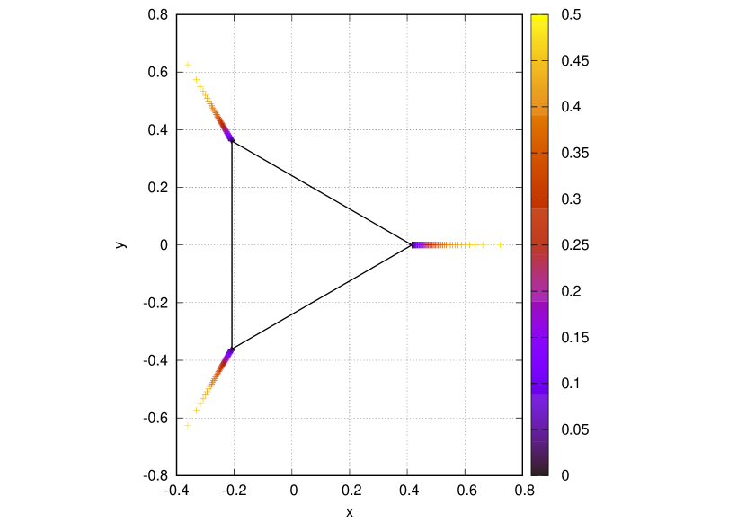
(a) Positive curvatures.

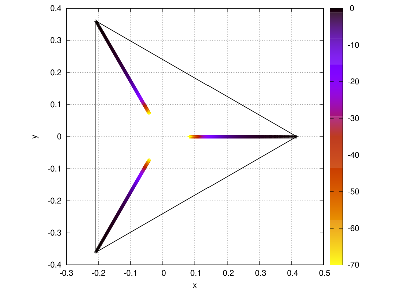
(b) Negative curvatures.

Figure 1: Continuation of Lagrange’s equilateral relative equilibrium $a$ with equal masses $m_{1}=m_{2}=m_{3}=1$. Lagrange’s equilateral relative equilibrium $a$ is marked with a black triangle. Relative equilibria continuating for curved spaces are color-coded according to their curvature value $\kappa$.

Using this methodology, we can numerically continue this relative equilibrium to spaces of constant curvature $\kappa\in[-70,0.48]$. The family of relative equilibria obtained is shown in Figure 1. All configurations shown verify the relative equilibrium condition (13) with precision $10^{-13}$.

When continuing to positive curvature, the family cannot be continued beyond $\kappa\approx 0.48$, possibly due to a bifurcation: this is an interesting question that we will try to answer in a forthcoming paper. When continuing to negative curvature, on the other hand, the family can be continued up to $\kappa\approx-70$ and beyond. We conjecture that the family actually extends to $\kappa\to-\infty$. However, we loose numerical accuracy as the relative equilibrium approaches the origin. In practice, we decided to stop our continuation when the numerical accuracy falls below $10^{-13}$.

5.3.2 Different Masses

Consider now Lagrange’s equilateral triangle on the plane, but assume three different masses, for example $m_{1}=1$, $m_{2}=2$, $m_{3}=3$. It is not hard to find this relative equilibrium analytically, given the following constrains:

1. The triangle is equilateral.

2. The length of each side must fulfill equation (7).

3. The center of mass is at the origin.

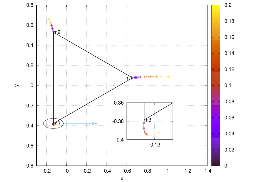
(a) Positive curvatures. Inset: magnification of the region about $m_{3}$.

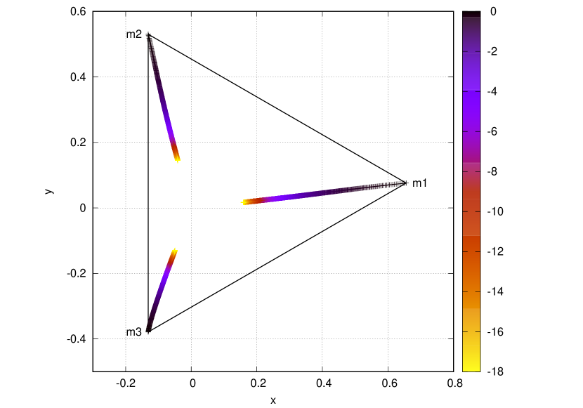
(b) Negative curvatures.

Figure 2: Continuation of Lagrange’s equilateral relative equilibrium $a$ with different masses $m_{1}=1$, $m_{2}=2$, $m_{3}=3$. Lagrange’s equilateral relative equilibrium $a$ is marked with a black triangle. Relative equilibria continuating for curved spaces are color-coded according to their curvature value $\kappa$.

Using the same methodology, we can numerically continue this relative equilibrium to spaces of constant curvature $\kappa\in[-18,0.19]$. The family of relative equilibria obtained is shown in Figure 2. All configurations shown verify the relative equilibrium condition (13) with precision $10^{-13}$.

When continuing to positive curvature, the family cannot be continued beyond $\kappa\approx 0.19$, possibly due to a bifurcation. When continuing to negative curvature, on the other hand, the family can be continued up to $\kappa\approx-18$ and beyond. We conjecture that the family actually extends to $\kappa\to-\infty$. However, we loose numerical accuracy as the relative equilibrium approaches the origin. In practice, we decided to stop our continuation when the numerical accuracy falls below $10^{-13}$.

5.3.3 Configurations in the sphere and hyperboloid

The inverse transformation of the stereographic projection [16, 8] defines the cartesian coordinates $(x,y,z)$ in the inertial frame of reference. The equation that must be fulfilled, due to the restriction that the particles move on the sphere or hyperboloid, is $x^{2}+y^{2}+\sigma z^{2}=\sigma R^{2}$, $\kappa=\sigma/R^{2}$, where $\sigma=1$ for the sphere, and $\sigma=-1$ for the hyperboloid.

In order to show all the configurations with the same curvature sign on a common surface, we rescale the configurations. Configurations with curvature $\kappa>0$ are rescaled in such a way that they lie on the surface of the unitary sphere $x^{2}+y^{2}+z^{2}=1$. Configurations with $\kappa<0$ are rescaled so that $x^{2}+y^{2}-z^{2}=-1$.

For positive curvature, the family that emerges from Lagrange’s equilateral triangle central configuration is shown in Figure 3. For comparison we plot the case of equal masses $m_{1}=m_{2}=m_{3}=1$ and different masses $m_{1}=1$, $m_{2}=2$, $m_{3}=3$ in the same figure. In a similar way, the central configurations for negative curvature are shown in Figure 4.

Under the rescaling, the families of central configurations share, in some sense, features with the the classical case: for a given curvature $\kappa$, if one body is more massive than other one then the body with more mass will be closer to the axis $z$ (in the classical case $z=0$, and the point of reference is the center of mass of the system), therefore also closer to the pole. This property can be appreciated in Figures 5, 6 for positive and negative curvatures, respectively. We remark that this is the opposite that happens without the rescaling. For instance, in the case of positive curvature we have the relation $\kappa=1/R^{2}$, therefore $R\to 0$ as $k\to\infty$.

As proved in [9], Lagrange’s equilateral solutions exist on spaces of constant curvature if and only if the three masses are equal and lie in a circle parallel to the equator. We remark that, until now, there were no results about relative equilibria where the three bodies have different masses and move on circles with different heights $z$ [6].

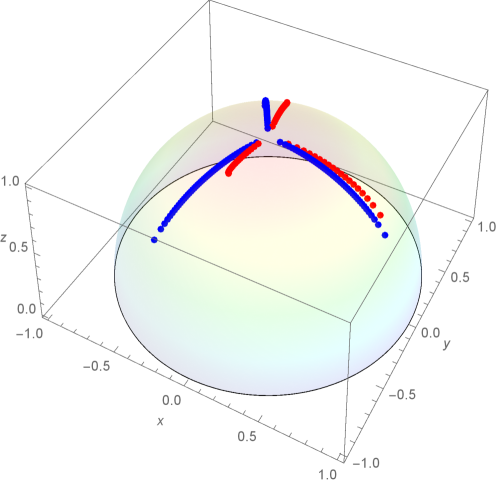
Figure 3: Continuation of Lagrange’s relative equilibrium $a$ in cartesian coordinates $(x,y,z)$ with positive curvature $\kappa=1/R^{2}$. Blue series for $m_{1}=1$, $m_{2}=1$, $m_{3}=1$, and red series for $m_{1}=1$, $m_{2}=2$, $m_{3}=3$. The configuration is rescaled in such a way that $x_{j}^{2}+y_{j}^{2}+z_{j}^{2}=1$ for $j=1,2,3$, and the reflection $z\to-z$ is used.

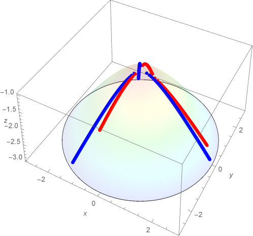
Figure 4: Continuation of Lagrange’s relative equilibrium $a$ in cartesian coordinates $(x,y,z)$ with negative curvature $\kappa=-1/R^{2}$. Blue series for $m_{1}=1$, $m_{2}=1$, $m_{3}=1$, and red series for $m_{1}=1$, $m_{2}=2$, $m_{3}=3$. The configuration is rescaled in such a way that $x_{j}^{2}+y_{j}^{2}-z_{j}^{2}=-1$ for $j=1,2,3$, and the reflection $z\to-z$ is used.

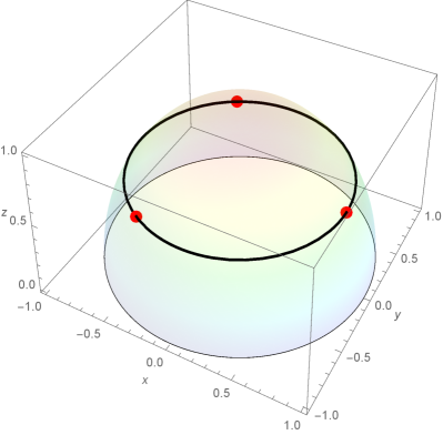
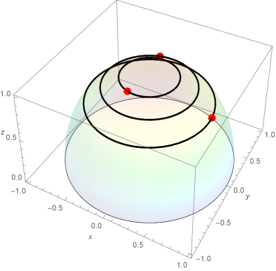
Figure 5: Periodic circular orbits on the sphere. On the left the case $m_{1}=1$, $m_{2}=1$, $m_{3}=1$, with $\kappa=0.49$, and on the right $m_{1}=1$, $m_{2}=2$, $m_{3}=3$, with $\kappa=0.19$. Same rescaling and reflection as in Figure 3.

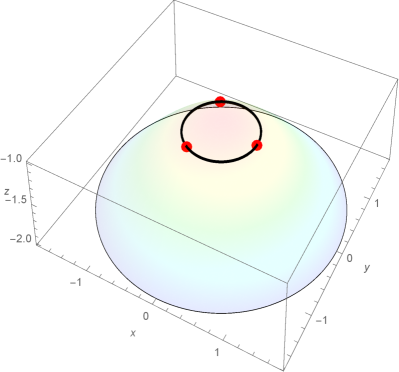
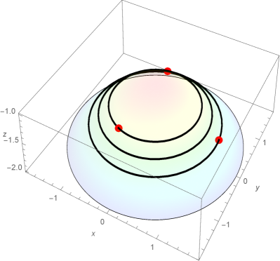
Figure 6: Periodic circular orbits on the hyperboloid. On the left the case $m_{1}=1$, $m_{2}=1$, $m_{3}=1$, with $\kappa=-0.49$, and on the right $m_{1}=1$, $m_{2}=2$, $m_{3}=3$, with $\kappa=-1.99$. Same rescaling and reflection as in Figure 4.

Acknowledgements

The first and third authors have been partially supported by Asociación Mexicana de Cultura A.C. and by CONACYT, México, project A1S10112. Research of P.R. was partially supported by NSF grant DMS-1814543. C.G.A. was partially supported by UNAM-PAPIIT project IN115019.

References

• [1] Sicardy B. Stability of the triangular lagrange points beyond gascheau’s value. Celest Mech Dyn Astr, 107(3):145–155, 2010.
• [2] Bizyaev Ivan A. Borisov Alexey V., Mamaev Ivan S. The spatial problem of two bodies on the sphere. reduction and stochasticity. Reg. Chaotic Dyn., 21(5), 2016.
• [3] Mamaev I.S. Montaldi J. Borisov A.V., Garcia-Naranjo L.C. Reduction and relative equilibria for the $2$-body problem in spaces of constant curvature. Cel. Mech. Dyn. Astr., 130:article 43, 2018.
• [4] Martínez R. Simó C. On the stability of the lagrangian homographic solutions in a curved three-body problem. Disc. Cont. Dyn. Sys., 33(3):1157–1175, 2013.
• [5] Martínez R. Simó C. Relative equilibria of the restricted three body problem in curved spaces. Cel. Mech. Dyn. Astr., 128:221–259, 2017.
• [6] Florin Diacu. Polygonal homographic orbits of the curved $n$–body problem. T. Am. Math. Soc., 364(5):2783–2802, 2011.
• [7] Florin Diacu. Relative equilibria of the Curved $N$–Body Problem. Atlantis Press, first edition, 2012.
• [8] Florin Diacu, Ernesto Pérez-Chavela, and J. Guadalupe Reyes Victoria. An intrinsic approach in the curved $n$-body problem: the negative curvature case. J. Differential Equations, 252(8):4529–4562, 2012.
• [9] Florin Diacu, Ernesto Pérez-Chavela, and Manuele Santoprete. The $n$-body problem in spaces of constant curvature. Part I: Relative equilibria. J. Nonlinear Sci., 22(2):247–266, 2012.
• [10] Routh E.J. On laplace’s three particles, with a supplement on the stability of steady motion. Proc. London Math. Soc., 6(86), 1875.
• [11] M. Fontaine and C. García-Azpeitia. Braids of the $n$-body problem by cabling a body in a central configuration. arXiv:1906.07702.
• [12] Gascheau G.. Examen d’une classe d’équations différentielles et applications à un cas particulier du problème des trois corps. C. R. Acad. Sci., 16:393, 1843.
• [13] C. García-Azpeitia and J. Ize. Global bifurcation of polygonal relative equilibria for masses, vortices and dNLS oscillators. J. Differential Equations, 251(11):3202–3227, 2011.
• [14] Pérez-Chavela E. Rodríguez-Olmos M. García-Naranjo L.C., Marrero J.C. Classification and stability of relative equilibria for the two-body problem in the hyperbolic space of dimension 2. J. Diff. Eq., 260:6375–6404, 2016.
• [15] F. J. Muñoz Almaraz, E. Freire, J. Galán, E. Doedel, and A. Vanderbauwhede. Continuation of periodic orbits in conservative and Hamiltonian systems. Phys. D, 181(1-2):1–38, 2003.
• [16] Ernesto Pérez-Chavela and J. Guadalupe Reyes-Victoria. An intrinsic approach in the curved $n$-body problem. The positive curvature case. Trans. Amer. Math. Soc., 364(7):3805–3827, 2012.
• [17] Sánchez-Cerritos J. Pérez-Chavela E. Hyperbolic relative equilibria for the negative curved n-body problem. Commun. Nonlinear Sci. Number Simulat, 67:460–479, 2019.
• [18] Sánchez-Cerritos J. Pérez-Chavela E. Regularization of the restricted (n+1)-body problem on curved spaces. Astr. Space Sci., 364:article 170, 2019.
• [19] Donald G. Saari. Collisions, Rings and Other Newtonian $N$–Body Problems. CBMS Regional Conference Series in Mathematics, 104, AMS, first edition, 2005.