A Multifactorial Optimization Paradigm for Linkage Tree Genetic Algorithm

Abstract

Linkage Tree Genetic Algorithm (LTGA) is an effective Evolutionary Algorithm (EA) to solve complex problems using the linkage information between problem variables. LTGA performs well in various kinds of single-task optimization and yields promising results in comparison with the canonical genetic algorithm. However, LTGA is an unsuitable method for dealing with multi-task optimization problems. On the other hand, Multifactorial Optimization (MFO) can simultaneously solve independent optimization problems, which are encoded in a unified representation to take advantage of the process of knowledge transfer. In this paper, we introduce Multifactorial Linkage Tree Genetic Algorithm (MF-LTGA) by combining the main features of both LTGA and MFO. MF-LTGA is able to tackle multiple optimization tasks at the same time, each task learns the dependency between problem variables from the shared representation. This knowledge serves to determine the high-quality partial solutions for supporting other tasks in exploring the search space. Moreover, MF-LTGA speeds up convergence because of knowledge transfer of relevant problems. We demonstrate the effectiveness of the proposed algorithm on two benchmark problems: Clustered Shortest-Path Tree Problem and Deceptive Trap Function. In comparison to LTGA and existing methods, MF-LTGA outperforms in quality of the solution or in computation time.

1 Introduction

Linkage Tree Genetic Algorithm has been shown to scale excellently on a variety of discrete, Cartesian-space, optimization problems [1, 2]. Linkage Tree Genetic Algorithm (LTGA) determines the linkages between problem variables in the population, then clusters relevant variables to build a linkage tree. In each generation, the linkage tree is used to create crossover masks to prevent disruption between high-quality linked genes, and different partial structures of two good parent solutions can be juxtaposed to construct a new good solution. LTGA performs well in various problems: Permutation Flowshop Scheduling Problem [2, 3], Nearest-neighbor NK landscapes [4], MAX-SAT problem [5, 6], Deceptive trap function [7], Multidimensional Knapsack Problem [8], etc. and outperforms traditional Genetic Algorithm (GA). However, the linkage tree is built from a single combinatorial optimization problem without transferred knowledge from other relevant problems.

Combinatorial optimization problems in real-life like Jobs scheduling, Cloud computing etc. require solving many tasks simultaneously. Arising from the need to solve a large number of user requests in Cloud Computing, Multifactorial Evolutionary Algorithm (MFEA) proposed by Gupta, et al. [9] can solve multiple independent optimization problems simultaneously using a single population of solutions in the unified search space. The unified search space encompasses the shared knowledge for all of the tasks and the knowledge belonging to the particular optimization task. Transferring knowledge between different tasks occurs through adjusting and exchanging shared genetic material in the unified search space. In the process of transferring knowledge, good partial solutions of each task are used to support the others tasks. Leveraging the supportive genetic material requires calculating the commonality between all tasks for effective knowledge transfer.

Inspired by the idea of Multifactorial Optimization (MFO) and LTGA, we exploit the advantages of crossover mechanism of LTGA and the implicit genetic transferring of MFO. We adopt the idea that many problems are represented in the unified search space, building linkage tree for each task exploits the knowledge from the other tasks. In particular, the linkage tree indicates the distances between problem variables. These variables corresponding to each problem are the partial structure of individuals in the shared representation. The distance between two sets of variables indicates the dependence between them, calculated.

In this paper, we introduce Multifactorial Linkage Tree Genetic Algorithm (MF-LTGA) by combing the main features of LTGA and MFO: Linkage tree is used to determine the relationship between problems variables, which is used to leverage shared information among optimization problems. The assortative mating step is modified to combine crossover mechanism of LTGA and vertical cultural transmission of MFEA: A linkage tree is selected corresponding to a particular task then the crossover operator is applied to generate new offspring based on that linkage tree. The vertical cultural transmission in MF-LTGA serves to transfer the phenotype of parents to their offspring.

The effectiveness of MF-LTGA is shown in comparison to LTGA and existing algorithms on the canonical Clustered Shortest-Path Tree Problem (CluSPT) [10] and Deceptive Trap Function (DTF). The results indicate that MF-LTGA is superior to LTGA in computation time, and quality of the solution.

The main contributions of this paper are:

• We propose a mechanism combining key features of LTGA and MFO, which we call MF-LTGA.

• We modify process for building the linkage tree based on unified search space to exploit both information between problem variables and transfer knowledge of independent tasks.

• We introduce an assortative mating mechanism to enhance the compatibility between the main features of MFO and LTGA.

• We propose a crossover operator to keep the key advantages of MFO and LTGA as well as maintain population diversity.

• The experimental results show that the our algorithm is more efficient than existing methods.

This paper is organized as follows. Section 2 introduces related works. A background of MFO and LTGA are briefed in Section 3. Section 4 describes the MF-LTGA algorithm. Section 5 presents and discusses experimental results. The paper concludes in Section 6 with discussions of the future extension of this research.

2 Related works

Linkage Tree Genetic Algorithm (LTGA) was introduced by Thierens [11] and is one of the newest variants of Evolutionary Algorithm (EA) [12, 13]. LTGA learns the linkage between the problem variables and groups of variables by building a hierarchical clustered tree using a proximity distance metric. In each generation, LTGA builds a linkage tree and then uses that tree to generate new offspring. LTGA has been successfully applied to various types of problems which we review next.

In [1], LTGA was proposed to solve permutation optimization problems by employing the random key encoding of permutations. To evaluate the dependency between two variables, two factors were proposed: the first factor, called relative-ordering information, focuses on the order of two genes while the second factor, called adjacency information, focuses on the proximity of the two genes.

In [11], LTGA is applied to solve the deceptive $mk-trap$ function. The authors use the mutual information for evaluating the dependency between variables and build the linkage tree of a population of solutions.

In [14], Goldman,  et al. introduced a benchmark problem, deceptive step trap problem for testing LTGA. To reduce the time complexity when calculating the entropy between all possible clusters, the authors also proposed the linkage between clusters. Instead of finding the entropy of an entire cluster, the new measure only finds the entropy between all pairs of independent problem variables in the population.

To improve the convergence of LTGA, Bosman, et al. [15] proposed Forced Improvements which is used when a solution cannot be improved. A different linkage model, Linkage Neighbors (LN) was also proposed. An advantage of the LN model compared to the Linkage Tree model is that it is well-suited to represent overlapping linkage relations.

Recently, the concept of Multifactorial Optimization (MFO) [16, 17] has been introduced in [9] as a new optimization paradigm toward evolutionary multitasking with a single population of individuals. In contrast to traditional evolutionary search paradigm, MFO conducts evolutionary search concurrently on multiple search spaces corresponding to the optimization problems, each possessing a unique function landscape. The efficacy of MFO has been confirmed by a set of continuous and combinatorial optimization problems in [18, 2, 19].

MFO has been applied to various algorithms which we review next. Feng, et al. [20] proposed two new mechanisms for combining Multifactorial Evolutionary Algorithm (MFEA) with Particles Warm Optimization Algorithm (PSO) (called MFPSO), Differential Evolution Algorithm (DE) (called MFDE). In the new algorithms, the authors designed new assortative mating schemes while the other components such as unified individual representation, vertical cultural transmission, etc., are kept the same as in the original MFEA.

Xie, et al. [21] introduced a hybrid algorithm combining MFEA and PSO (call HMFEA) in which PSO plays the role of local search in the MFEA. A difference between HMFEA and the original MFEA is that the PSO is added after genetic operation of MFEA and applied to the intermediate-pop in each generation. To adjust dynamically the velocity and guarantee that the convergence velocity is not too fast, an adaptive variation adjustment factor $g_{\alpha}$ is proposed. The factor $g_{\alpha}$ is used to control the velocity of each particle.

In [22], Wen and Ting combine the MFEA with Genetic Programming (GP) for learning an ensemble of decision trees. In this algorithm, each task is associated with one run of GP. To generate diverse decision trees, their algorithm further scrambles the dataset for each task by randomly mapping the feature indexes. The tasks will then work on the dataset with different feature sequences.

Zhong. et al. [23] proposed a multifactorial GP (MFGP) paradigm toward evolutionary multitasking GP. MFGP consists of a novel scalable chromosome encoding scheme and new evolutionary mechanisms for MFO based on self-learning gene expression programming.

Although MFO and LTGA were developed for solving various type of problems, there have been no studies that combine the strengths of MFO and LTGA into a new algorithm. Therefore, this paper proposes mechanisms to take the advantages of both MFO and LTGA into a new algorithm. The experimental results demonstrate the effectiveness of the new algorithm.

3 Preliminaries

This section provides a brief background of the Multifactorial Optimization paradigm and the Linkage Tree Genetic Algorithm.

3.1 Multifactorial Optimizations

In [9], Gupta et al. introduced Multifactorial Optimization as an evolutionary multi-tasking paradigm that optimizes multiple tasks simultaneously. Unlike traditional methods, MFO solves multiple tasks within only a single task. To achieve this, individuals are represented in unified search space and MFO calculates the skill of individual and splits the population into different groups: each individual is placed in the group corresponding to the task it performs best. The ability to solve problems in multitasking environments not only allows MFO to utilize genetic materials created in a specific group but also useful for another task.

To evaluate an individual, Gupta et al. [9] define the following properties for every individual $p_{i}$ in population P:

• Factorial Cost: The factorial cost $\psi^{i}_{j}$ of an individual $p_{i}$ on task $T_{j}$ is computed by its fitness or objective value on a particular task $T_{j}$.

• Factorial rank: Factorial rank $r^{i}_{j}$ is the rank of $p_{i}$ on task $T_{j}$, relative to all other individuals in P.

• Scalar Fitness: Scalar fitness $\varphi_{i}$ of $p_{i}$ is based on its best rank over all tasks; i.e. $\varphi_{i}$ = 1/min{$r^{i}_{1}$, $r^{i}_{2}$, …, $r^{i}_{K}$}.

• Skill Factor: Skill factor $\tau_{i}$ of $p_{i}$ is the one task, amongst all other tasks in MFO, with which the individual is associated. This may be defined as $\tau_{i}=argmin_{j}\{r^{i}_{j}\}$.

In order to calculate fitness of an individual, individuals are decoded in different tasks to obtain “Factorial Cost”. Individuals are evaluated by its correlation with other individuals based on “Factorial Cost” to find the most suitable task called “Skill Factor”.

3.2 Linkage Tree Genetic Algorithm

Recently, a powerful linkage-learning EA, LTGA, was proposed by Dirk Thierens [11]. LTGA maximizes the effectiveness of the crossover operator through discovering and exploiting the relationship between problem variables during the evolutionary searching. To store linkage information, LTGA uses an additional hierarchical tree, called linkage tree. A cluster of problem variables that LTGA believes to be linked is represented by a node in the linkage tree. In each generation, the linkage tree is rebuilt by selecting a set of solutions from the current population before determining the relationship between problem variables in that set.

3.2.1 Constructing Linkage Tree

LTGA aims to identify the variables that make a dependent set, then uses an agglomerative hierarchical clustering algorithm to proceed bottom-up. Hierarchical clustering algorithm constructs Linkage information between variables, and stores it as a Linkage Tree. Each node in the Linkage Tree is a cluster of genes that are close to each other. At its first stage, the algorithm considers each gene to be a dependent cluster, before repeatedly joining the two closest clusters to create a bigger one until all genes are in the same cluster. The size of population may impact the accuracy of the information the linkage tree represents. The larger the population size, the higher the possibility of good solutions appearing in it. Therefore, the linkage tree constructed from larger population may better reflect the relations between the genes. However, for larger population, the construction of linkage tree would be more consuming in terms of computational resources and the number of evolutionary operations on each generation would be higher. Hence, it is necessary to choose an appropriate population size in order to keep a balance between the linkage information accuracy and computational resources consumption.

The details are shown in Algorithm 1:

Input: A set of solutions from the current population

Output: A Linkage tree

1 Compute the proximity matrix using metric $D$.

2 Assign each variable to a single cluster.

3 Repeat until one cluster left:

4  Join two closest clusters $C_{i}$ and $C_{j}$ into $C_{ij}$.

5  Remove $C_{i}$ and $C_{j}$ from the proximity matrix.

6  Compute the distance between $C_{ij}$ and all clusters.

7  Add cluster $C_{ij}$ to the proximity matrix.

Algorithm 1 Hierarchical Clustering

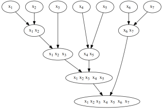
Figure 1: An example of hierarchical clustering algorithm on 7 genes.

An example of hierarchical clustering is shown in Figure 1: The first two closest genes $x_{1}$ and $x_{2}$ are joined into a cluster $x_{1}x_{2}$, clusters $x_{1}$, $x_{2}$ are removed from the proximity matrix. In the next iteration, LTGA considers the distances between the new cluster $x_{1}x_{2}$ and the other clusters, then combines the closest pair of clusters from the current population. After each generation, LTGA rebuilds the linkage tree from current population.

3.2.2 Crossover operator

Each cluster in the Linkage Tree is used as a crossover mask, the variables in a cluster are swapped between parent pair to generate two new offspring. If one of the offspring is better than its parents, then those offspring become parents for the next crossover for the remaining crossover masks. LTGA performs operations through $2l-1$ clusters in Linkage Tree, the order of visiting clusters to perform crossover operations impacts the quality of the final solution.

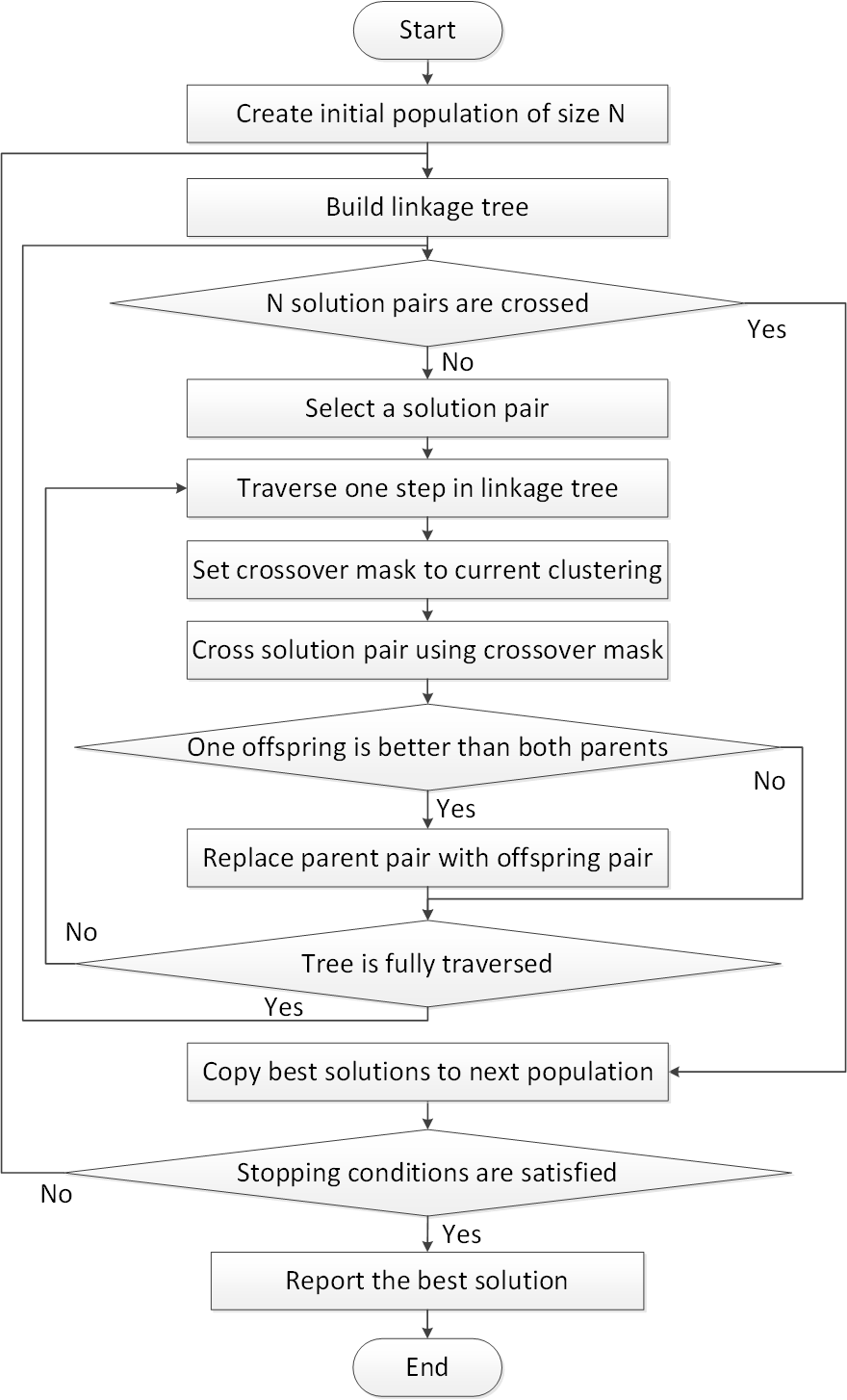
Figure 2: The outline of Linkage Tree Genetic Algorithm

The outline of Linkage Tree Genetic Algorithm is presented in Figure 2.

4 Multifactorial Optimization with Linkage Tree Genetic Algorithm

In this section, we introduce the combination of Multifactorial Optimization (MFO) and Linkage Tree Genetic Algorithm (LTGA) which we call Multifactorial Linkage Tree Genetic Algorithm (MF-LTGA).

MFO is designed for conducting multitasking with the exchange of information among individuals through two key components: assortative mating and vertical cultural transmission. In a standard genetic algorithm and MFO, the solution representation and the crossover operator need to be designed to achieve good solution. However, this design will be difficult to achieve if there is insufficient domain knowledge. Different from the genetic algorithm, LTGA possesses unique solution reproduction and update operations through linkage models which learn the relationship between the problems variable through estimation of distribution.

MF-LTGA is our proposal by combining LTGA and MFO in order to capture the advantages of both algorithms to improve the quality of the solution. To hybridize MFO and LTGA, new assortative mating schemes are required. In addition, some operators like unified individual representation, vertical cultural transmission, etc., also need to change to adapt to LTGA. The workflow in Figure 3 describes the outline of our proposed algorithm, in which we maily focus on the two steps: build linkage tree and perform associative mating based on linkage tree. MF-LTGA start with a initial population of individuals which is presented in a unified search space. The assortative mating of MF-LTGA serves as the genetic operator to reproduce next generation as well as Multifactorial Evolutionary Algorithm (MFEA). However, the assortative mating of MF-LTGA is performed based on linkage tree which learns a probabilistic model of the current population of solutions. In addition, unlike MFEA, vertical cultural transmission is determined in assortative mating because it depends on tree selection. The pseudo code of MF-LTGA is presented in Algorithm 2. In what follows, the design of the MF-LTGA is detailed.

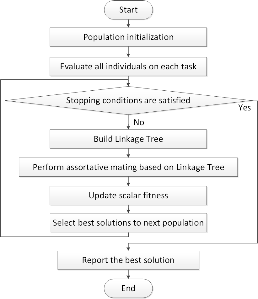
Figure 3: The scheme of Multifactorial Linkage Tree Genetic Algorithm

1Generate an initial population of size $n$;

2 Evaluate all individuals on every task in the multi-tasking environment, and obtain the skill factor of each individual;

3 $t\leftarrow 0$;

4 while stopping conditions are not satisfied do

5       Build linkage tree $\triangleright$ Refer to Algorithm 3;

6       Perform assortative mating based on linkage model on current-pop to generate an intermediate-pop $\triangleright$ Refer to Algorithm 4;

7       Update the scalar fitness of all the individuals in intermediate-pop $\triangleright$ Refer subsection 3.1;

8       Select the fittest individuals from intermediate-pop to form the next generation;

9       $t\leftarrow t+1$;

10      

11 end while

Algorithm 2 MF-LTGA

4.1 Linkage Tree Building

A key strength of LTGA is its ability to learn the relationship between the problem variables. To maintain this strength when applied to a multi-tasking environment, either a linkage tree is built for all tasks, or linkage trees are built separately for each task. Building only a single tree for all tasks can not provide the dependency between the variables because the relationship between two variables in one task might be different from that in another task. Therefore, this paper applies the second approach. The pseudo code of the building linkage tree in MF-LTGA is given in Algorithm 3.

In Algorithm 3, for each task, we firstly generate a selected population including individuals whose Skill Factor is in that task. Next, each individual in the selected population is decoded to a solution for this task which will be added to a population, called task-population. Finally, linkage tree is built based on task-population in the same way in [11].

Input: $P$: A population of individuals in unified search space; $k$: Number of tasks.

Output: Linkage tree $T_{i}$ for task $i,i=1,\ldots,k$.

1 foreach task $i$ do

2       Choose individuals from $P$ which have skill factor of task $i$ to generate selected-population ($C$);

3       Decode all individuals of selected-population ($C$) to generate task-population ($P_{i}$);

4       Build the linkage tree (${T_{i}}$) based on task-population ($P_{i}$);

5 end foreach

return $T_{i},i=1,\ldots,k$

Algorithm 3 Linkage tree building in MF-LTGA

4.2 Assortative Mating

The pseudo code of the assortative mating in MF-LTGA is given in Algorithm 4. Firstly, current-population is partitioned into pairs of individuals which are considered as parents. Next, with each pairs of parents, we select randomly a single task for evaluation, because evaluating every individual for every problem being solved will often be computationally too expensive. However, comparisons and evaluations only on selected task may lead to a loss on good individuals of unselected tasks. These individual that has unselected skill factor might be an outstanding solution for that particular task and could produce good offspring on that task. Therefore, we need to create a backup population which contains the individuals that does not have their skill factor tasks selected. Next, the pair of parents will have crossover operator applied based on the tree of the selected task to generate offspring. As a result, the offspring imitate selected task, so that vertical cultural transmission is integrated into the assortative mating. Finally, offspring-pop and backup-pop are concatenated to form an intermediate-pop.

Input:

• $P$: A population of individuals in unified search space;

• $k$: Number of tasks;

• Linkage tree $T_{i}$ for task $i,i=1,\ldots,k$.

Output: A new population of individuals in unified search space

1 Build a set of selected parents ($S$) by randomly partitioning population ($P$) into pairs of individuals;

2 foreach pair ($p_{i},p_{j}$) in $S$ do

3       $\tau_{i}\leftarrow$ skill factor of $p_{i}$;

4       $\tau_{j}\leftarrow$ skill factor of $p_{j}$;

5       $\tau\leftarrow\tau_{i}$;

6       if $\tau_{i}\neq\tau_{j}$ then

7             $\tau\leftarrow$ A random skill factor from $\{\tau_{i},\tau_{j}\}$;

8             if $\tau=\tau_{i}$ then

9                   Add $p_{j}$ to backup population ($B$);

10                  

11             end if

12            else

13                   Add $p_{i}$ to backup population ($B$);

14                  

15             end if

16            

17       end if

18      Parents $p_{i}$ and $p_{j}$ crossover in task $\tau$ based on $T_{\tau}$ to generate two offspring $o_{i}$ and $o_{j}$ $\triangleright$ Refer to Algorithm 5;

19       Two offspring $o_{i}$ and $o_{j}$ imitates selected skill factor $\tau$ ;

20       Add best individual of $\{o_{i},o_{j}\}$ to offspring population ($O$);

21      

22 end foreach

23Concatenate offspring-pop and backup-pop to form an intermediate-pop ($O\cup B$);

24 return intermediate-pop;

Algorithm 4 Assortative Mating in MF-LTGA

4.3 Crossover Operator

In this part, we will clarify the crossover operator based on linkage tree. The pseudo code of the crossover operator is presented in Algorithm 5. In the new crossover operator, we traverse the linkage tree top-down to set the crossover mask. With each mask, parent pair is crossed using crossover mask to generate a pair of offspring which is evaluated on the selected task to compete with the parent pair. If one of the children is better than both parents then the offspring pair replaces the parent pair, and MF-LTGA continues to traverse the linkage tree with the new pair. If none of the two children is better than their parents, MF-LTGA continues its tree traversal with the parent pair. However, after some traversal in the tree, some individuals cannot be improved. Therefore, we propose a mechanism for replacing these individuals by new individuals. Whenever an individual cannot be improved, we will punish this individual; once the individual’s punishment record reaches the threshold, it is replaced by a new individual.

Input:

• Parents $p_{i}$ and $p_{j}$;

• $max_{p}$: maximum punishment;

• Linkage tree $T_{\tau}$ for task $\tau$;

Output: Two offspring $o_{i}$ and $o_{j}$;

1 change $\leftarrow$ False;

2 $n_{p}\leftarrow$ 0;

3 foreach node $t_{i}$ in $T_{\tau}$ do

4       Set crossover mask to node $t_{i}$;

5       Cross parents $p_{i}$ and $p_{j}$ using crossover mask to generate offspring $o_{i}$ and $o_{j}$;

6      

7      if one offspring better than both parents then

8             Replace parents $p_{i}$ and $p_{j}$ by offspring $o_{i}$ and $o_{j}$;

9             change $\leftarrow$ True;

10            

11       end if

12      

13 end foreach

14if !change then

15       $n_{p}\leftarrow n_{p}$ + 1;

16       if $n_{p}>max_{p}$ then

17             Replace parents $p_{i}$ and $p_{j}$ by two new random individuals;

18             $n_{p}\leftarrow$ 0;

19            

20       end if

21      change $\leftarrow$ False;

22      

23 end if

24

25return Two offspring $o_{i}$ and $o_{j}$;

Algorithm 5 Crossover Operator in MF-LTGA

5 Simulation results

We evaluate the performance of MF-LTGA on two canonical problems: Clustered Shortest-Path Tree Problem (CluSPT) [10, 24] and Deceptive Trap Function (DTF) [4, 11]. These two problems are described in detail later in this section.

5.1 Evaluation criteria

We focus on the following criteria to assess the quality of the output of the algorithms.

Criteria
Average (Avg)	Average function value over all runs.
Best-found (BF)	Best function value achieved over all runs.
Num.Opt	The number of optimal solutions are found.
Num.Eval	Number of evaluations to success.

We compare the performance of algorithms via a normalized difference. More specifically, let $C_{A}$ and $C_{B}$ denote the performance of algorithms A and B under metric C; then the relative performance of algorithm A relative to that of algorithm B is defined as

$PI(A,B)=\dfrac{C_{B}-C_{A}}{C_{B}}*100\%$

As examples: C could denote the cost of the best solution found by an algorithm, or the average number of evaluations needed to obtain a solution.

To evaluate the performance of the MF-LTGA in solving the CluSPT and the DTF, we implemented three sets of experiments.

• In the first set, the quality of the solutions obtained by the C-MFEA [25] and E-MFEA [26] on each instance were compared with those obtained by MF-LTGA.

• In the second set, various experiments were performed to analyze possible influencing factors.

• In the third set, analyze the effective of MF-LTGA on instances of the Deceptive Trap Function.

This paper uses the decoding method and evolutionary operators in [25].

Each problem instance was evaluated 30 times for the CluSPT and 10 times for the DTF on Intel Core i7-3.60GHz, 16GB RAM computer using Windows 8 64-bit. The source codes of LTGA and MF-LTGA were written in the Python.

The simulation parameters include population size = 100, number of evaluations = $10^{6}$, probability of random mating = 0.5, mutation rate = 0.05 and number of tasks = 2.

5.2 Deceptive Trap Function

The Deceptive Trap Function is a well-known canonical benchmark for LTGA. With $m$-Trap Functions, the number of local optima of the deceptive trap function is $2^{m}-1$. A notable point for this problem is that a hillclimbing algorithm quickly becomes trapped in one of the local optima while Genetic Algorithm (GA) will quickly converge to the deceptive local optima [11].

5.2.1 Problem formulation

The Deceptive mk-Trap Function (mk-DTF) is a binary, additively decomposable function composed of $m$ trap functions $DT_{i}$, each defined on a separate group of $k$ bits (the total length is $l=mk$). The cost of mk-DTF is defined as:

$$f_{mk-DTF}(x_{1}\ldots x_{l})=\sum_{i=0}^{m-1}DT_{i}(x_{ik}\ldots x_{ik+k-1})$$ (1)

with $x_{i}\in\{0,1\}$

Call $u$ the number of bits in such a group that are equal to 1:

$$DT_{i}(x_{ik}\ldots x_{ik+k-1})=\begin{cases}k,&\text{if }u=k\\ k-1-u,&\text{otherwise}\end{cases}$$ (2)

Clearly, the array of all 1-bits is the global optimal solution of the mk-DTF and all schemata of order less than $k$ are deceptive.

5.2.2 Experimental setup

The MF-LTGA is tested on deceptive functions with trap length $k$ = 4, 5, 6. The number of blocks $m$ varies from 5 to 30 with increments of 5, the problem length thus varies from 20 to 180. The details of problem instances and parameters are presented in Table 1.

Table 1: mk-DTF Instances and Parameters for Evaluating MF-LTGA and LTGA

k	3	3	3	3	3	3	4	4	4
m	5	10	15	20	25	30	5	10	15
Problem length	15	30	45	60	75	90	20	40	60
Population size	128	128	128	128	128	128	128	128	128
k	4	4	4	5	5	5	5	5	5
m	20	25	30	5	10	15	20	25	30
Problem length	80	100	120	25	50	75	100	125	150
Population size	128	128	128	256	256	256	256	256	256

Each problem instance was evaluated 10 times on Intel Core i7-3.60GHz, 16GB RAM computer using Windows 8 64-bit.

5.2.3 Experimental results

Table 2 presents the results obtained by two algorithms LTGA and MF-LTGA. The results on this table indicate that LTGA slightly outperforms MF-LTGA: LTGA gets optimal solutions in all 100 tests while MF-LTGA only finds optimal results in 99 out of 100 tests.

Table 2: mk-DTF Results Obtained By MF-LTGA and LTGA

. LTGA MF-LTGA k m Num.Opt Num.Evals Num.Opt Num.Evals P.Imp 3 5 10 4,228.0 10 2783.2 34.2% 3 10 10 13,664.8 10 8908.8 34.8% 3 15 10 24,552.0 10 13780.8 43.9% 3 20 10 34,007.6 10 23434.8 31.1% 3 25 10 52,244.0 10 28179.2 46.1% 3 30 10 57,387.2 10 39765.2 30.7% 4 5 10 7706.4 10 6642.4 13.8% 4 10 10 25615.2 10 23587.2 7.9% 4 15 10 39010.8 10 38043.2 2.5% 4 20 10 64053.2 10 61209.2 4.4% 4 25 10 85021.2 10 66013.2 22.4% 4 30 10 111479.2 10 95200.0 14.6% 5 5 10 20342.4 10 13900.8 31.7% 5 10 10 66150.0 10 49568.4 25.1% 5 15 10 123994.4 10 65327.2 47.3% 5 20 10 176378.4 9 145569.6 17.5% 5 25 10 231582.4 10 128116.8 44.7% 5 30 10 284411.2 10 196322.4 31.0% Num.Opt: The number of optimal solutions are found. Num.Eval: The Average number of evaluations to success. P.Imp: The percentage of differences between the average number of evaluations to success.

However, the number of evaluations needed to find successfully the optimal solutions of MF-LTGA is smaller than that of LTGA in all instances, and nearly 18% fewer on average. This difference climbs up to 47.3% on the test case $k=5,m=15$. Detailed comparisons are given in Figure 4 in which Num.Evals denotes number of evaluations needed to find successfully the optimal solutions.

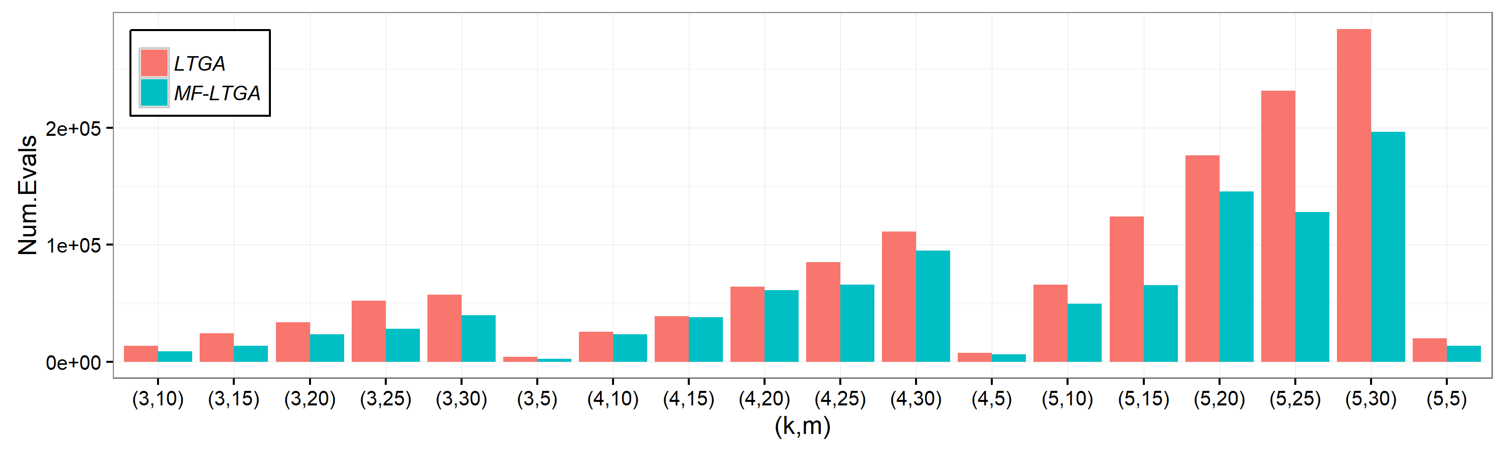
Figure 4: Comparing number of evaluations needed to find success the optimal solutions

5.3 Clustered Shortest-Path Tree Problem

5.3.1 Problem formulation

In this paper, we let $G=(V,E,w)$ represent a simple, connected and undirected graph, with vertex set $V$, edge set $E$, and non-negative edge weights $w$, respectively. An edge between vertices $u$ and $v$ is denoted by $(u,v)$, and its weight is denoted by $w(u,v)$.

For a vertex subset $U$, the sub-graph of $G$ induced by $U$ is denoted by $G[U]$. A collection $C~{}=~{}\{C_{i}|1\leq i\leq k\}$ of subsets of $V$ is a partition of $V$ if the subsets are mutually disjoint and their union is exactly $V$. A path in $G$ is simple if no vertex appears more than once on the path. This paper only considers simple paths.

For a given spanning tree $T$ of $G=(V,E,w)$ and $u,v\in V$, let $d_{T}(u,v)$ denote the shortest path length between $u$ and $v$ on $T$.

The CluSPT problem [10] is defined as following

Input:	- A weighted undirected graph $G=(V,E,w)$.
	- Vertex set $V$ is partitioned into $k$ clusters ${C_{1},C_{2},...,C_{k}}$.
	- A source vertex $s\in V$.
Output:	- A spanning tree $T$ of $G$.
	- Sub-graph $T[C_{i}](i=1,\ldots,k)$ is a connected graph.
Objective:	$\displaystyle\sum_{v\in V}d_{T}(s,v)\rightarrow$ min

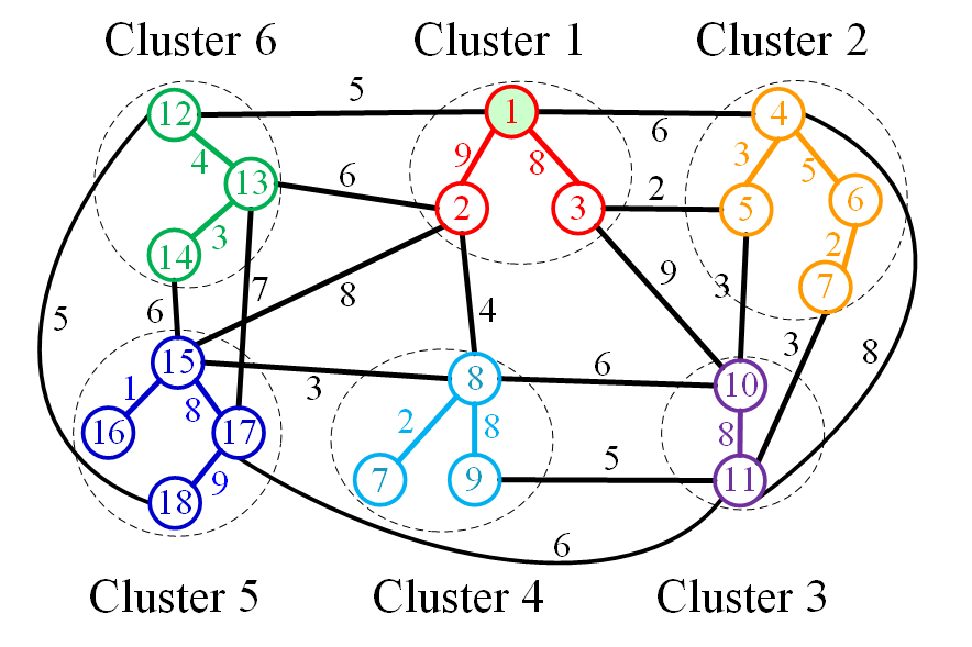
(a)

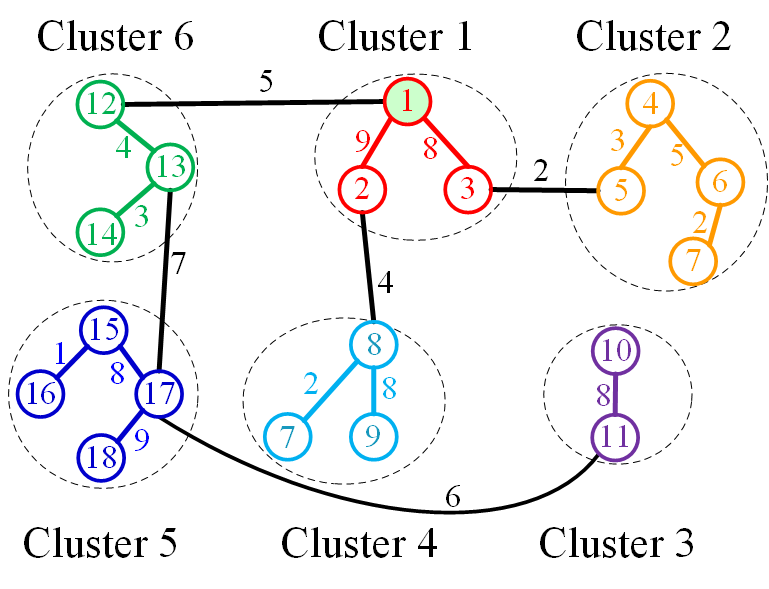
(b)

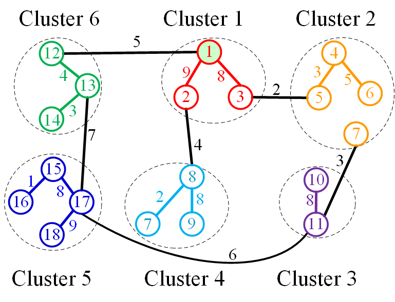
(c)

Figure 5: An example of valid and invalid solutions for the CluSPT

Figure 5 illustrates the cases of valid and invalid solutions of CluSPT. Figure 5(a) shows the input graph G with 6 clusters, 18 vertices and vertex 1 as source vertex. Figure 5(b) presents a valid solution of CluSPT. In Figure 5(c), the vertex 6 and vertex 7 in cluster 2 are not connected, so this solution violates the second condition of the output of the CluSPT problem.

5.3.2 Problem instances

For assessment of the proposed algorithms’ performance, we created instances for CluSPT from Clustered Traveling Salesman Problem (CluTSP) instances [27, 28] by adding the information of the source vertex. The main reason for building CluSPT instances from CluTSP instances was that CluTSP instances have been proved to be suitable for clustered problems in general [28].

All tested instances are available via [29]

5.3.3 Experimental results

Comparison between the performance of existing algorithms and that of MF-LTGA

In this section, we compare the results obtained by C-MFEA [25] and E-MFEA [26] with those achieved by MF-LTGA. Tables 4, 5 and 6 illustrate the results obtained by these algorithm on instances of Type 1, Type 5 and Type 6. In table 6, the symbol “-” indicates that the corresponding instances were not executed by C-MFEA.

The results in Table 4, 5 and 6 point out that both single-tasking (ST) and multitasking (MT) outperform both E-MFEA and C-MFEA in most test cases. In particular, both MT and ST outperformed the two existing algorithms on all test cases in Type 5. Table 3 summarizes the comparison results among E-MFEA, C-MFEA, ST and MT on the benchmarks.

Table 3: Comparison of results obtained by MF-LTGA and the existing algorithms.

Algorithm		Type 1	Type 5	Type 6	Total
	Number of instances in a Type	18	14	20	52
C-MFEA	Number of instances on which MF-LTGA outperformed C-MFEA	13	14	12	39
	Maximum PI(MF-LTGA, C-MFEA)	36.30%	25.90%	32.10%
E-MFEA	Number of instances on which MF-LTGA outperformed E-MFEA	9	14	15	38
	Maximum PI(MF-LTGA, E-MFEA)	28.20%	29.30%	34.20%
LTGA	Number of instances on which MF-LTGA outperformed LTGA	13	10	17	42
	Maximum PI(MF-LTGA, LTGA)	2.50%	2.70%	3.30%

The experimental results point out that MT is also better than ST on approximately 68% of the test cases i.e., 17 out of 26 Type 1 instances, 10 out of 14 Type 5 instances and 25 out of 36 Type 6 instances. Maximum PI(MT, ST) are 2.5% (for Type 1), 2.7% (for Type 5) and 3.3% (for Type 6).

The experimental results obtained by C-MFEA, E-MFEA and MF-LTGA on Type 1 instances are shown in Table 4. On this set of instances, MT outperforms ST on 13 out of 18 instances (values in red). C-MFEA and E-MFEA outperforms ST on 3 and 9 out of 18 instances (values in italics). C-MFEA and E-MFEA outperforms MT on 5 and 9 out of 18 instances respectively (values in bold).

The results on Type 6 instances are displayed in Table 6. ST outperformed C-MFEA on 10 out of 12 instances and outperformed E-MFEA on 15 out of 20 instances.

Convergence trends

We use the functions in [9] for computing the normalized objectives and averaged normalized objectives, and analyze the convergence trends of the proposed algorithm.

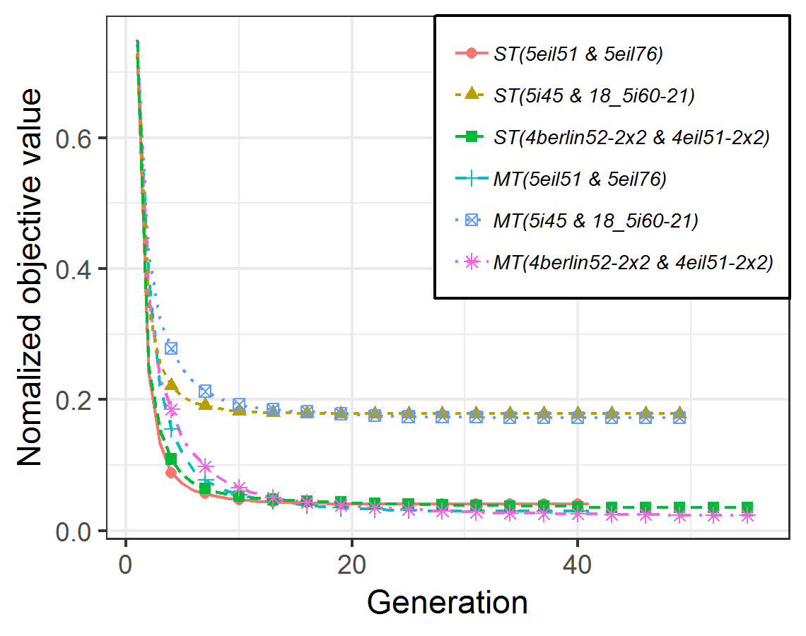
Figure 6: Convergence trends of $\tilde{f}$ in multi-tasks and serial single task for instances 10eil51 and 10eil76 in Type 1; instances 10i60-21 and 10i65-21 in Type 5; instances 4berlin52-2x2 and 4eil51-2x2 in Type 6.

Figure 6 illustrates the convergence trends of the ST and MT for instances 10eil51 and 10eil76 in Type 1; instances 10i60-21 and 10i65-21 in Type 5; instances 4berlin52-2x2 and 4eil51-2x2 in Type 6. These figures point out that the convergence rate of MT is faster than that of ST in most test cases.

A notable point in Figure 6 is that the numbers of evaluations of each generation are proportional to the dimensionalities of the instances. Moreover, in this experiment, the number of evaluations of each generation is a constant parameter. Due to this reason, the number of generations among instances might vary.

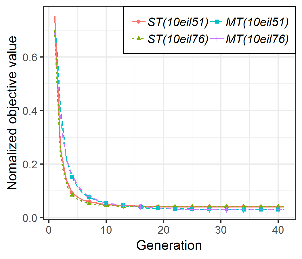
(a)

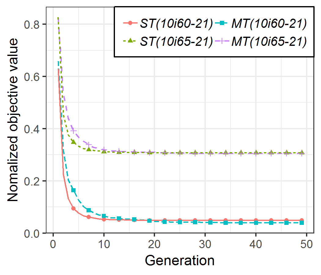
(b)

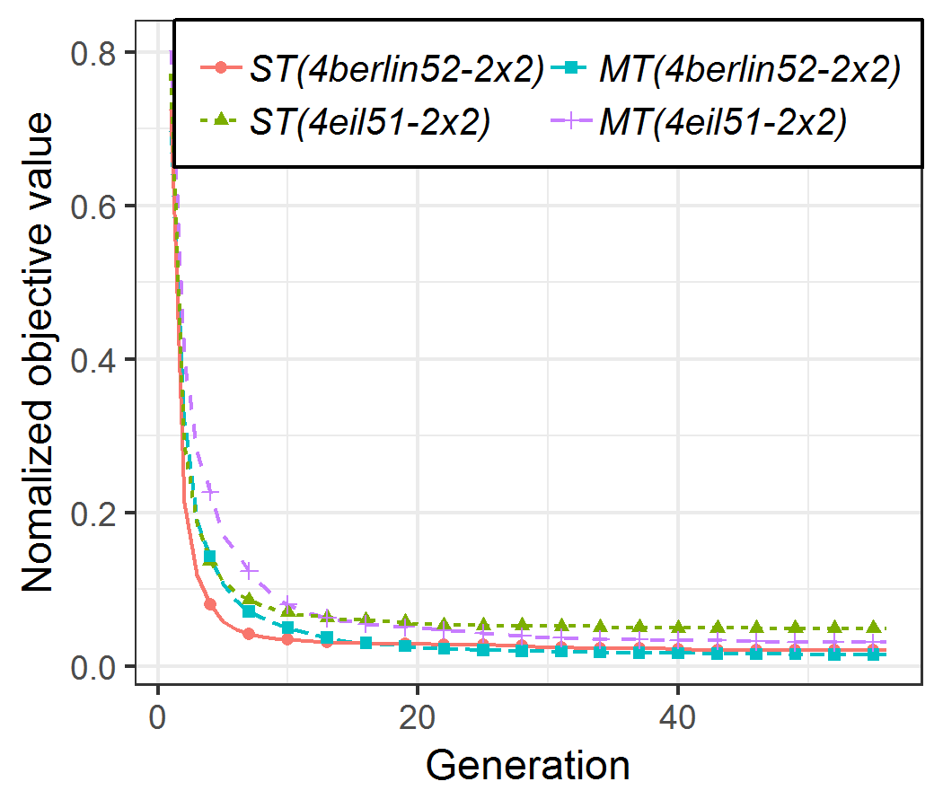
(c)

Figure 7: Comparing convergence trends of $\tilde{f_{1}}$ and $\tilde{f_{2}}$ in multi-tasks and serial single task for instances 10eil51 and 10eil76 in Type 1; instances 10i60-21 and 10i65-21 in Type 5; instances 4berlin52-2x2 and 4eil51-2x2 in Type 6.

The major convergence trends of those algorithms in Figure 6 is that MT converges slower than ST for initial generations but MT surpasses ST in later generations which means that the implicit genetic transferring among tasks in evolutionary multitasking paradigm improves the convergence speed of MT in comparison with ST

Figure 7 provides insight into the improved performance as a consequence of MT. The figure depicts the convergence trends corresponding to each individual task, which is somewhat similar to that of MT and ST in Figure 6 when the convergence rate of each task in MT is better than the corresponding task in ST in later generations.

6 Conclusion

This paper introduced a mechanism for combining LTGA and MFO. The novel algorithm kept the main features of both LTGA and MFO, and descripted new methods for building Linkage Tree Model, Assortative Mating and Crossover Operator. The experimental results show that the newly proposed algorithms were more effective in solving the canonical CluSPT and DTF compared with some other existing meta-heuristics.

Several theoretical aspects of the MF-LTGA will be investigated in more detail. In the future, we will focus on methods for constructing only one Linkage Tree Model for all tasks.

Table 4: Results Obtained By E-MFEA, C-MFEA, LTGA and MF-LTGA on Instances In Type 1

Instances	E-MFEA		C-MFEA		LTGA		MF-LTGA
	BF	Avg	BF	Avg	BF	Avg	BF	Avg
10berlin52	46185.8	46707.8	48569.8	48569.8	44269.0	45071.3	44331.3	44869.7
10eil51	2008.3	2039.4	1891.7	1891.7	1787.5	1861.2	1726.2	1829.4
10eil76	2775.4	2973.3	2489.5	2489.5	2296.0	2505.6	2324.7	2442.3
10kroB100	198181.6	218275.1	170695.2	170695.2	151186.8	158277.4	147780.3	156804.6
10pr76	643903.6	665835.1	632704.5	632704.5	551924.2	579248.6	533900.2	566138.2
10rat99	10427.6	10792.8	8937.1	8937.1	7778.2	8412.0	7904.5	8323.5
15eil51	1662.9	1781.4	1922.0	1922.0	1984.6	2130.4	2019.9	2099.7
15eil76	3349.0	3402.8	3773.0	3773.0	3305.0	3496.0	3318.9	3436.6
15pr76	772173.1	787889.0	833734.0	833734.0	814795.5	835549.4	808406.1	829608.7
15st70	4972.1	5117.7	5171.8	5171.8	4362.2	4522.5	4335.8	4435.4
25eil101	5192.4	5248.4	6852.3	6852.3	4828.9	4983.8	4852.9	4950.5
25kroA100	164038.4	167528.9	266798.7	266798.7	163607.8	171118.9	165696.9	170175.5
25lin105	106500.2	107524.2	182650.4	182650.4	133620.8	141926.3	136782.0	139844.5
25rat99	9234.7	9375.8	12931.7	12931.7	8072.6	8417.5	8213.1	8446.7
50eil101	3978.2	3991.2	9461.1	9461.1	7985.5	8150.7	12356.2	12378.8
50kroA100	173626.5	176321.3	451952.5	451952.5	289992.4	298047.5	525968.7	527328.5
50kroB100	138019.5	138849.1	450713.7	450713.7	236715.1	245304.7	538061.6	538991.1
50lin105	147967.2	148332.6	309399.9	309399.9	226340.0	232625.7	392391.3	392750.7

Table 5: Results Obtained By E-MFEA, C-MFEA, LTGA and MF-LTGA on Instances In Type 5

Instances	E-MFEA		C-MFEA		LTGA		MF-LTGA
	BF	Avg	BF	Avg	BF	Avg	BF	Avg
10i120-46	119168.5	120920.6	105754.4	125137.1	98742.1	101766.7	97389.6	101961.4
10i45-18	26065.2	27515.4	26942.8	32663.5	24209.2	25404.1	23739.6	24727.7
10i60-21	43125.9	45389.1	37640.0	45427.1	34424.5	37629.5	34424.5	37346.9
10i65-21	46456.5	48420.7	41053.9	49824.3	39137.4	41928.4	39511.7	41965.8
10i70-21	49875.8	51532.2	41892.8	55760.2	38714.6	42618.6	39506.1	41476.8
10i90-33	61567.6	64955.9	55361.9	65493.1	54402.0	57278.2	55186.4	57545.4
5i45-18	20042.8	22345.5	15511.5	17007.0	14986.9	16063.1	15068.7	15792.3
5i60-21	35099.9	36474.5	29797.9	34613.0	29263.8	31129.9	29113.7	30500.8
5i65-21	33648.4	35663.9	31517.4	34235.2	31238.8	33537.1	31829.7	33180.1
5i70-21	43816.9	49519.0	35746.0	39302.4	35096.6	38044.7	35706.8	37763.8
5i75-22	37992.7	40668.9	34867.3	38705.1	35700.9	38396.4	35361.8	37813.2
5i90-33	62701.2	65622.1	53230.6	55888.2	53195.0	56485.3	53592.2	56604.4
7i60-21	44669.6	46337.4	37690.6	41532.3	36692.9	40318.7	37186.7	40062.7
7i65-21	45237.3	47211.2	35878.8	40222.5	36230.3	38858.5	35924.4	38116.1

Table 6: Results Obtained By E-MFEA, C-MFEA, LTGA and MF-LTGA on Instances In Type 6

Instances	E-MFEA		C-MFEA		LTGA		MF-LTGA
	BF	Avg	BF	Avg	BF	Avg	BF	Avg
10berlin52-2x5	31659.1	33590.6	-	-	35643.0	37342.1	36449.8	37222.8
12eil51-3x4	1922.1	1960.9	2185.0	2691.5	1782.7	1867.3	1749.8	1826.5
12eil76-3x4	3352.2	3449.3	3065.7	3896.1	2852.6	2938.8	2752.4	2892.6
12pr76-3x4	664562.6	685351.9	-	-	720063.9	767947.9	713144.0	751440.1
12st70-3x4	4750.9	4795.7	-	-	4265.6	4391.7	4619.6	4753.3
15pr76-3x5	601015.9	623645.7	-	-	763415.0	838763.6	778422.9	815522.3
16eil51-4x4	1371.3	1425.9	-	-	1779.3	1843.7	1775.8	1814.1
16eil76-4x4	2314.0	2374.9	-	-	2705.3	2836.7	2569.5	2772.3
16lin105-4x4	179729.7	179729.7	-	-	160926.8	170624.9	161710.3	166233.5
16st70-4x4	3560.4	3560.4	-	-	3248.9	3481.6	3235.8	3369.7
4berlin52-2x2	35413.1	37121.5	23635.3	24751.0	23287.9	24664.1	23509.9	24431.5
4eil51-2x2	2545.3	2641.1	1909.5	2053.9	1934.7	2058.0	1911.6	2010.3
4eil76-2x2	4319.3	4517.2	2949.1	3179.9	2977.2	3231.6	3023.5	3198.8
4pr76-2x2	688228.2	762880.2	446862.4	480043.8	450274.6	513032.1	461545	546392.3
6pr76-2x3	741847.3	771563.7	656978.3	736743.5	661240.6	703446.5	655261.7	694048.9
6st70-2x3	3880.5	4057.0	3508.1	4244.1	3501.1	3764.2	3522.32548	3729.8
9eil101-3x3	4281.2	4585.0	3320.3	4345.8	3292.9	3545.5	3334.0	3501.9
9eil51-3x3	2127.0	2182.7	2106.5	2630.8	1954.5	2073.5	1942.8	2036.8
9eil76-3x3	3599.5	3730.8	3401.8	4048.0	3059.1	3253.1	3091.1	3225.8
9pr76-3x3	713966.7	749030.6	642796.6	783056.1	576233.6	599439.8	576233.6	599439.8

References

- [1] P. A. Bosman, N. H. Luong, D. Thierens, Expanding from Discrete Cartesian to Permutation Gene-pool Optimal Mixing Evolutionary Algorithms, in: Proceedings of the 2016 on Genetic and Evolutionary Computation Conference, ACM, 2016, pp. 637–644.
- [2] A. Bouter, T. Alderliesten, C. Witteveen, P. A. Bosman, Exploiting linkage information in real-valued optimization with the real-valued gene-pool optimal mixing evolutionary algorithm, in: Proceedings of the Genetic and Evolutionary Computation Conference, ACM, 2017, pp. 705–712.
- [3] G. H. Aalvanger, N. H. Luong, P. A. N. Bosman, D. Thierens, Heuristics in Permutation GOMEA for Solving the Permutation Flowshop Scheduling Problem, in: A. Auger, C. M. Fonseca, N. Lourenço, P. Machado, L. Paquete, D. Whitley (Eds.), Parallel Problem Solving from Nature – PPSN XV, Springer International Publishing, 2018, pp. 146–157.
- [4] D. Thierens, P. A. Bosman, Evolvability analysis of the linkage tree genetic algorithm, in: International Conference on Parallel Problem Solving from Nature, Springer, 2012, pp. 286–295.
- [5] R. de Bokx, D. Thierens, P. A. Bosman, In Search of Optimal Linkage Trees, in: Proceedings of the Companion Publication of the 2015 Annual Conference on Genetic and Evolutionary Computation, ACM, 2015, pp. 1375–1376.
- [6] K. L. Sadowski, P. A. Bosman, D. Thierens, On the usefulness of linkage processing for solving MAX-SAT, in: Proceedings of the 15th annual conference on Genetic and evolutionary computation, ACM, 2013, pp. 853–860.
- [7] D. Thierens, The linkage tree genetic algorithm, in: International Conference on Parallel Problem Solving from Nature, Springer, 2010, pp. 264–273.
- [8] J. P. Martins, C. M. Fonseca, A. C. Delbem, On the performance of linkage-tree genetic algorithms for the multidimensional knapsack problem, Neurocomputing 146 (2014) 17–29.
- [9] A. Gupta, Y.-S. Ong, L. Feng, Multifactorial evolution: toward evolutionary multitasking, IEEE Transactions on Evolutionary Computation 20 (3) (2016) 343–357.
- [10] M. D’Emidio, L. Forlizzi, D. Frigioni, S. Leucci, G. Proietti, On the Clustered Shortest-Path Tree Problem., in: ICTCS, 2016, pp. 263–268.
- [11] D. Thierens, Linkage tree genetic algorithm: first results, in: Proceedings of the 12th annual conference companion on Genetic and evolutionary computation, ACM, 2010, pp. 1953–1958.
- [12] E. E. Agoston, Introduction to Evolutionary Computing, Berlin, Springer-Verlag, 2003.
- [13] T. Back, Evolutionary algorithms in theory and practice: evolution strategies, evolutionary programming, genetic algorithms, Oxford university press, 1996.
- [14] B. W. Goldman, D. R. Tauritz, Linkage tree genetic algorithms: variants and analysis, in: Proceedings of the 14th annual conference on Genetic and evolutionary computation, ACM, 2012, pp. 625–632.
- [15] P. A. Bosman, D. Thierens, Linkage neighbors, optimal mixing and forced improvements in genetic algorithms, in: Proceedings of the 14th annual conference on Genetic and evolutionary computation, ACM, 2012, pp. 585–592.
- [16] Y.-S. Ong, A. Gupta, Evolutionary multitasking: a computer science view of cognitive multitasking, Cognitive Computation 8 (2) (2016) 125–142.
- [17] T. B. Trung, L. T. Thanh, L. T. Hieu, P. D. Thanh, H. T. T. Binh, Multifactorial Evolutionary Algorithm For Clustered Minimum Routing Cost Problem, 2019, pp. 170–177.
- [18] P. A. Bosman, D. Thierens, On measures to build linkage trees in LTGA, in: International Conference on Parallel Problem Solving from Nature, Springer, 2012, pp. 276–285.
-
[19]
P. D. Thanh, H. T. T. Binh, T. B. Trung,
An efficient strategy for
using multifactorial optimization to solve the clustered shortest path tree
problem, Applied Intelligencedoi:10.1007/s10489-019-01599-x.
URL https://doi.org/10.1007/s10489-019-01599-x - [20] L. Feng, W. Zhou, L. Zhou, S. Jiang, J. Zhong, B. Da, Z. Zhu, Y. Wang, An empirical study of multifactorial pso and multifactorial de, in: Evolutionary Computation (CEC), 2017 IEEE Congress on, IEEE, 2017, pp. 921–928.
- [21] T. Xie, M. Gong, Z. Tang, Y. Lei, J. Liu, Z. Wang, Enhancing evolutionary multifactorial optimization based on particle swarm optimization, in: Evolutionary Computation (CEC), 2016 IEEE Congress on, IEEE, 2016, pp. 1658–1665.
- [22] Y.-W. Wen, C.-K. Ting, Learning ensemble of decision trees through multifactorial genetic programming, in: Evolutionary Computation (CEC), 2016 IEEE Congress on, IEEE, 2016, pp. 5293–5300.
- [23] J. Zhong, L. Feng, W. Cai, Y.-S. Ong, Multifactorial Genetic Programming for Symbolic Regression Problems, IEEE Transactions on Systems, Man, and Cybernetics: Systems (99) (2018) 1–14.
- [24] M. D’Emidio, L. Forlizzi, D. Frigioni, S. Leucci, G. Proietti, Hardness, approximability, and fixed-parameter tractability of the clustered shortest-path tree problem, Journal of Combinatorial Optimization (2019) 1–20.
- [25] P. D. Thanh, D. A. Dung, T. N. Tien, H. T. T. Binh, An effective representation scheme in multifactorial evolutionary algorithm for solving cluster shortest-path tree problem, in: Evolutionary Computation (CEC), 2018 IEEE Congress on, IEEE, 2018, pp. 811–818.
- [26] H. T. T. Binh, P. D. Thanh, T. B. Trung, L. P. Thao, Effective multifactorial evolutionary algorithm for solving the cluster shortest path tree problem, in: Evolutionary Computation (CEC), 2018 IEEE Congress on, IEEE, 2018, pp. 819–826.
- [27] K. Helsgaun, Solving the Clustered Traveling Salesman Problem Using the Lin-Kernighan-Helsgaun Algorithm, Computer Science Research Report (142) (2011) 1–16.
- [28] M. Mestria, L. S. Ochi, S. de Lima Martins, GRASP with path relinking for the symmetric euclidean clustered traveling salesman problem, Computers & Operations Research 40 (12) (2013) 3218–3229.
- [29] P. D. Thanh, CluSPT instances, Mendeley Data v2, http://dx.doi.org/10.17632/b4gcgybvt6.2, 2018. doi:http://dx.doi.org/10.17632/b4gcgybvt6.2.