A detailed look at the stellar populations in green valley galaxies

Abstract

The green valley (GV) represents an important transitional state from actively star-forming galaxies to passively evolving systems. Its traditional definition, based on colour, rests on a number of assumptions that can be subject to non-trivial systematics. In Angthopo et al. (2019), we proposed a new definition of the GV based on the 4000Å break strength. In this paper, we explore in detail the properties of the underlying stellar populations by use of $\sim$230 thousand high-quality spectra from the Sloan Digital Sky Survey (SDSS), contrasting our results with a traditional approach via dust-corrected colours. We explore high quality stacked SDSS spectra, and find a population trend that suggests a substantial difference between low- and high-mass galaxies, with the former featuring younger populations with star formation quenching, and the latter showing older (post-quenching) populations that include rejuvenation events. Subtle but measurable differences are found between a colour-based approach and our definition, especially as our selection of GV galaxies produces a cleaner “stratification” of the GV, with more homogeneous population properties within sections of the GV. Our definition based on 4000Å break strength gives a clean representation of the transition to quiescence, easily measurable in the upcoming and future spectroscopic surveys.

1 Introduction

Our understanding of galaxy formation and evolution has greatly advanced over the past decades, especially thanks to high quality all-sky galaxy surveys. However, challenges lie ahead, due to the complex mixture of physical processes, the different timescales involved, and the inherent degeneracies in the interpretation of the observations. To tackle these hurdles, we have to combine numerical hydrodynamical simulations based on physical equations, with large galaxy surveys, where the large data sets allow us to carefully select samples, control systematics, and follow a general statistical approach. These surveys often combine photometric and spectroscopic data, enabling the discovery of fundamental relations such as a conspicuous bimodality (see, e.g., Strateva et al., 2001). The bimodal behaviour represents a clear divide regarding star formation activity (or stellar population age) with a strong dependence with stellar mass and cosmic age (see, e.g., Bell et al., 2004). This bimodality can be shown on various diagrams spanned by parameters such as the colour-magnitude (Graves et al., 2009), star formation rate (SFR) - mass (Schiminovich et al., 2007; Cibinel et al., 2013), UVJ bi-colour diagram (Williams et al., 2009), or colour-mass (Bremer et al., 2018; Schawinski et al., 2014), to name a few. The two contrasting galaxy populations have been termed the red sequence (hereafter RS), and the blue cloud (hereafter BC) in colour-mass diagrams. Inherent to this bimodal nature is the region separating BC from RS, commonly known as the green valley (hereafter GV, Salim, 2014).

By construction, the GV can be considered a region overlapping a number of possible evolutionary pathways between BC and RS, and various scenarios have been postulated to understand the observed distribution of galaxies (Faber et al., 2007). It is generally accepted that galaxies on the GV are undergoing quenching of their star formation activity (roughly “ascending” on a colour vs stellar mass diagram, where the colour index increases upwards), or undergoing rejuvenation events (Thomas et al., 2010) from recent infall of gas – therefore tracing a “descending” track on this diagram. Multiple survey-based studies have been carried out to assess the properties of GV galaxies. Martin et al. (2007) combined NUV and optical fluxes to define and study the GV, finding a significant increase in the fraction of AGN, with respect to BC or RS galaxies. The connection of AGN activity with quenching was further supported by the transition phases found in the population analysis of SDSS early-type galaxies made by Schawinski et al. (2007). However, a morphological analysis of GV galaxies revealed a complex mixture (Schawinski et al., 2014), leading to a scenario where, at least, two channels are present, with short quenching timescales ($\sim$100 Myr) being involved in the evolution of early-type galaxies, and longer timescales ($\sim$2-3 Gyr) in late-type systems (see also, Smethurst et al., 2015; Nogueira-Cavalcante et al., 2018). Phillipps et al. (2019) use MAGPHYS to extract star formation histories from GAMA GV galaxies to derive transition times $\sim$2–4 Gyr, with no specific signal that the quenching takes place faster than an otherwise decaying rate. Moreover, the transition processes appear to affect mostly the disk component, favouring secular disk fading (Bremer et al., 2018), and environment unsurprisingly affecting the appearance of the GV (Coenda et al., 2018). It is worth mentioning here that the presence of merger-like morphologies is not favoured in GV galaxies (Mendez et al., 2011). Also note that the GV transition times appear to proceed faster at high redshift, following the standard downsizing scenario (see, e.g., Gonçalves et al., 2012, for a study at z$\sim$0.8).

Regarding intrinsic colour distributions, it is found that GV galaxies present blue outer regions, so that the recent star formation responsible for their being GV galaxies may be caused by rejuvenation events from the infall of gas clouds or gas-rich smaller galaxies (Thilker et al., 2010; Salim & Rich, 2010; Fang et al., 2012). Alternatively, one can consider the quenching of star formation moving outwards from the centre due to gas depletion (Kelvin et al., 2018).

On the theoretical side, state-of-the-art numerical simulations of galaxy formation such as EAGLE are able to quantify quenching timescales (Wright et al., 2019) and the physical processes associated with quenching (Gabor et al., 2010). Through these simulations, they find that the quenching timescale is dependent on galaxy mass and environment. The simulations suggest that low-mass galaxies, M${}_{\star}<10^{9.6}$ M_⊙, feature quenching timescales $\gtrsim$3 Gyr, and intermediate mass galaxies, $10^{9.7}$ M${}_{\odot}<$M${}_{\star}<10^{10.3}$ M_⊙, have the longest quenching timescales, whereas the most massive galaxies, M${}_{\star}>10^{10.3}$ M_⊙ are estimated to have the shortest quenching timescales, $\tau\lesssim$2 Gyr. Moreover, quenching is faster in satellites, with respect to centrals (however see, Trayford et al., 2016). Note though, that alternative selection methods, such as using sub-millimeter fluxes, give rise to different morphologies of the same region (e.g. “green mountain”, Eales et al., 2018), reflecting the complexity of the interpretation of this transition region, and the potential biases caused by the specific details of the selection.

The wide range of timescales found suggests a mixture of evolutionary channels. At low mass, quenching may be mostly due to ram pressure stripping or stellar feedback, depending on whether the galaxies are satellites or centrals. Intermediate mass galaxies, with the highest quenching timescales, are thought to undergo radio-mode AGN and/or stellar feedback. Finally, at the massive end, major mergers that include strong AGN activity seem to be the main cause of quenching (Hopkins et al., 2006). Moreover, halo mass may also provide a valid mode of quenching in galaxies hosted by halos above a critical mass M${}_{\rm crit}\sim 10^{12}$ M_⊙ (Gabor et al., 2010). However, to further complicate our attempt at understanding the nature of GV galaxies, they are also likely to move from RS to GV or even into the BC. This can occur through events such as wet mergers, where a quiescent gas-poor galaxy merges with a star-forming gas-rich galaxy, so that the surplus of gas causes rejuvenation (Thomas et al., 2010). Events such as accretion of gas may also cause rejuvenation.

Due to the importance of the GV as a transition phase that can constrain the underlying physical processes, it is essential that we find an effective and robust definition of the GV, that is easily implemented in theoretical models of galaxy formation. Although many intriguing results have been observed using the colour-based definition of the GV, they may suffer from systematics caused by the adopted dust correction. The standard procedure (see, e.g., Brinchmann et al., 2004) compares a number of photometric and spectroscopic observables with a set of population synthesis models where a dust prescription is applied, assuming an extinction law fixed to constraints from Milky Way stars (Cardelli et al., 1989) or from starburst galaxies (Calzetti et al., 2000). This method appears to work quite well (Angthopo et al., 2019), however the results may be prone to uncontrolled systematics, especially given the observed correlation between the parameters that describe the effective attenuation by dust in star-forming galaxies (see, e.g. Kriek & Conroy, 2013; Tress et al., 2018; Salim et al., 2018; Narayanan et al., 2018).

This paper focuses on an analysis of the new selection of GV galaxies using the 4000Å break strength as proposed by Angthopo et al. (2019, hereafter A19). The 4000Å break is a highly sensitive age indicator defined over a relatively narrow spectral region (250Å using the definition of Balogh et al., 1999), to avoid a large effect from dust, but wide enough to be measured with relatively low S/N spectra, including low spectral resolution, as, e.g. with slitless grism data (Hathi et al., 2009) or medium band filters (Hernán-Caballero et al., 2013). Therefore, the break can be accurately measured at moderately low spectral resolution, opening its use to present and future medium spectral resolution surveys that use slitless grism spectroscopy, such as PEARS (Ferreras et al., 2009); FIGS (Pirzkal et al., 2017); Euclid (Laureijs et al., 2011); WFIRST (Spergel et al., 2015); or imaging surveys that use medium band passbands, such as ALHAMBRA (Aparicio Villegas et al., 2010); SHARDS (Pérez-González et al., 2013); JPAS (Benitez et al., 2014). The definition of the GV with the 4000Å break is expected to provide a more direct representation of the age distribution, with substantially weaker contamination from dust.

Hereafter, we refer to the GV selection via the 4000Å strength as “D4k sel”. We include a comparative study with a colour-based selection, via ${}^{0.1}(g-r)$ – hereafter defined as “${}^{0.1}(g-r)$ sel”. Note the colour is K-corrected to z=0.1, that represents the typical redshift of our SDSS-based sample. Section 2 outlines the survey used, as well as the creation of the spectral stacks used in the analysis of GV galaxies. Section 3 explores the stacks by use of line strengths and simple stellar population (SSP) models. Section 4 analyses the properties of GV galaxies using spectral fitting of composite populations. In Section 5 we discuss the main results, and Section 6 finishes with a summary.

2 Sample selection

2.1 Spectroscopic data

This paper continues the work presented in A19, based on a sample of spectroscopic data from the classic Sloan Digital Sky Survey (SDSS, York et al., 2000). We select the sample and retrieve the spectra from Data Release 14 (Abolfathi et al., 2018). SDSS is a full-sky survey that includes spectroscopic observations of galaxies with Petrosian $r$-band magnitude in the range 14.5$<r_{\rm AB}<$17.7. Our selection criteria identifies targets with relatively high signal-to-noise ratio, snMedian$\_$r$>$10. We stack the spectra within carefully defined regions on the plane that defines GV galaxies (see below).

Our GV is defined on a plane spanned by a stellar population parameter (i.e. either the 4000 Å break strength or a more standard broadband colour) along with velocity dispersion ($\sigma$), as measured in the SDSS fibre. $\sigma$ is preferred with respect to stellar mass, as it is directly measurable in good quality spectra, being free of the systematics associated with stellar mass estimates (such as the derivation of the total flux, or the model-dependent constraint of the stellar mass to light ratio). Furthermore, velocity dispersion is the observable that more strongly correlates with stellar population properties (see, e.g., Bernardi et al., 2003; Ferreras et al., 2019). The use of spectra with the imposed threshold in S/N guarantees a robust estimate of $\sigma$. Our sample is constrained in redshift between z=0.05 and 0.1, (median $0.077\pm 0.013$) resulting in $\sim$228,000 galaxies with high quality spectra. We bin the sample according to velocity dispersion from $\sigma$=70 km/s to 250 km/s, with bin spacing of $30\,$km/s.

The SDSS spectra cover the wavelength range 3800–9200 Å, with variable resolution, from R=1,500 at $\lambda$=3,800 Å, increasing to R=2,500 at $\lambda$=9,000 Å (Smee et al., 2013). The spectra are dereddend with respect to foreground extinction, adopting the standard Milky Way dust law (Cardelli et al., 1989). The correction required was determined by the extinction parameter $A_{g}$, quoted in the SDSS catalogues, evaluated in the $g$ band. Once the foreground dust correction is applied, the spectra are brought to the rest frame, and the individual estimates of the 4000Å break are measured, adopting the following definition (Balogh et al., 1999):

$${\rm D}_{n}(4000)=\frac{\langle\Phi^{R}\rangle}{\langle\Phi^{B}\rangle},\;{\rm where}\;\langle\Phi^{i}\rangle\equiv\frac{1}{(\lambda_{2}^{i}-\lambda_{1}^{i})}\int_{\lambda_{1}^{i}}^{\lambda_{2}^{i}}\Phi(\lambda)d\lambda$$ (1)

and $(\lambda_{1}^{B},\lambda_{2}^{B},\lambda_{1}^{R},\lambda_{2}^{R})=(3850,3950,4000,4100)$Å. Note that our definition contrasts with the traditional approach, originally defined by Bruzual (1983) that integrate $\Phi(\nu)$ in wavelength space. We believe our definition has an easier interpretation, as the flux ratio between two spectral intervals that straddle the 4000Å break. These two definitions can be compared via a rescaling with a constant factor $\sim$1.08 between the old and the new definition, irrespective of the properties of the underlying populations.

In this paper, as well as in A19, we contrast the newly defined GV with the traditional one based on colours from broadband photometry. We adopt ${}^{0.1}(g-r)$ as the reference colour, i.e. all galaxies are measured at a fiducial redshift z=0.1. The colours are taken from the flux ratios as measured within the 3 arcsec fibres of the SDSS classic spectrograph – to be consistent with the analysis of the observed spectra – and the K-correction needed to bring them to the fiducial redshift is measured directly from the spectra, following the standard approach (see, e.g. Hogg et al., 2002), adopting a vanilla-standard cosmology ($\Omega_{m}=0.3$; $\Omega_{\Lambda}=0.7$, $H=70$ km s^-1 Mpc^-1). As reference, our K-correction in $(g-r)$ stays below 0.14 mag (below 0.085 mag in 90% of the sample), and the median correction applied is $+0.04\pm 0.03$ mag. The colour is also corrected for intrinsic dust absorption, following the dust parameters of Kauffmann et al. (2003) and adopting the Calzetti et al. (2000) attenuation law. Note we use $A_{V}$ as baseline for the correction, where we find, at z=0.1, $A_{g}^{0.1}=1.16A_{V}^{0.1}$ and $A_{r}^{0.1}=0.88A_{V}^{0.1}$. We refer the reader to fig. 2 in A19 for a comparison between dust-corrected and uncorrected colours on the selection plane. Note the classic SDSS 3 arcsec diameter fibres map the central region of galaxies, $\sim$3-5 kpc. However the interpertation of our results are robust (see Appendix C for an analysis of aperture effects).

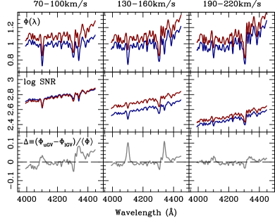
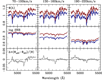
Figure 1: A comparison of the stacks is shown here in two important spectral windows: the neighbourhood of the H$\gamma$ and H$\delta$ absorption lines (left panels) and the region around the H$\beta$ and Mg+Fe complex (right panels). From top to bottom, the panels show the fluxes of the lGV (in blue) and the uGV (in red), with a small arbitrary vertical offset to avoid crowding; the signal to noise ratio on a logarithmic scale; and the relative flux difference between uGV and lGV spectra. The top labels show the velocity dispersion in each case. All stacks have been convolved to a common velocity dispersion equivalent of 235 km/s.

2.2 GV definition

We give here a brief description of the selection of GV galaxies, as proposed by A19, and refer interested readers to that paper for more details. Each galaxy is identified by two parameters: velocity dispersion ($\sigma$) and an indicator of stellar age (hereafter $\pi$), choosing either the 4000Å break strength, D_n(4000), or the dust-corrected colour, ${}^{0.1}(g-r)$. In addition, the sample is cross-matched with the JHU/MPA catalogue (Kauffmann et al., 2003) from which we retrieve the BPT classification of nebular emission lines (Baldwin et al., 1981). This enabled us to split the sample into unclassified/quiescent (BPT=$-$1), star-forming (BPT=1,2), composite (BPT=3), Seyfert (BPT=4) and LINER (BPT=5) galaxies. We do not consider here those spectra classified as composite (BPT=3), for a cleaner classification of the three regions. Moreover, the definition of the GV, as shown below, only relies on quiescent and star-forming galaxies. In each velocity dispersion bin, we fit separately the distribution of star-forming (SF) and quiescent (Q) galaxies adopting a Gaussian distribution with respect to $\pi$, namely:

$${\cal P}_{k}(\pi;\sigma)\equiv\frac{1}{s_{k}(\sigma)\sqrt{2\pi}}e^{-\frac{1}{2}\left[\frac{\pi-\mu_{k}(\sigma)}{s_{k}(\sigma)}\right]^{2}},$$ (2)

where $\mu_{k}(\sigma)$ and $s_{k}(\sigma)$ are, respectively, the mean and the standard deviation of the distribution of $\pi$ corresponding to galaxies in the velocity dispersion bin given by $\sigma$. We now propose the ansatz that these Gaussian distributions be interpreted as the probability distribution function (PDF) of blue cloud galaxies (for $k$=SF) and red sequence galaxies (for $k$=Q). Once the PDFs are defined for the BC and RS, the green valley subset is assumed to follow a probability distribution function given by:

$${\cal P}_{\rm GV}(\pi;\sigma)\equiv\frac{1}{s_{\rm GV}(\sigma)\sqrt{2\pi}}e^{-\frac{1}{2}\left[\frac{\pi-\mu_{\rm GV}(\sigma)}{s_{\rm GV}(\sigma)}\right]^{2}},$$ (3)

where the width of the Gaussian is chosen

$$s_{\rm GV}(\sigma)=\frac{1}{2}s_{\rm Q}(\sigma),$$ (4)

and the mean is given by

$${\cal P}_{\rm SF}[\mu_{\rm SF}(\sigma);\sigma]={\cal P}_{\rm Q}[\mu_{\rm Q}(\sigma);\sigma].$$ (5)

We emphasize these constraints are purely empirical and defined ad hoc. The constraint on the mean implies that at the peak of the GV PDF, a BC galaxy and a RS galaxy are indistinguishable from a probabilistic point of view. The constraint on the width ensures that the GV does not include large fractions of galaxies in the BC or RS regions. Note that this method is performed independently within each velocity dispersion bin. The actual selection of GV galaxies follows a Monte Carlo sampling method. For each galaxy within a given velocity dispersion bin, a uniform random deviate ($r$) is obtained between 0 and 1, and the galaxy is accepted into the GV subset if ${\cal P}_{\rm GV}[\pi;\sigma]>r$. The probability distribution functions obtained for the six velocity dispersion bins can be found in fig. 1 of A19. The GV set is further split into an upper- (uGV), middle- (mGV) and lower- (lGV) green valley, defined by the terciles of the distribution of $\pi$ in the GV sample within each velocity dispersion bin. Table 1, in the appendix, shows the number of galaxies in the uGV and lGV within each velocity dispersion bin and the fraction of galaxies according to their BPT flag. For reference, we include in the table the results when colour is not corrected with respect to intrinsic dust attenuation.

2.3 Spectral Stacking

The subsamples of GV galaxies are then used to produce high quality stacked spectra. High S/N is needed for a robust analysis of the stellar population content. However, more importantly, our motivation to stack the spectra is to average out galaxy-to-galaxy variations, leading to a set of “super-spectra” for which the variations between different regions of the selection plane are only caused by the transitional mechanisms that give rise to the BC/GV/RS distribution.

We follow the standard procedure for the stacking of the SDSS spectra (see, e.g. Ferreras et al., 2013). The stacking was carried on spectra that were de-reddened and brought to a rest-frame wavelength in the air system, applying a normalisation according to the median flux in the rest-frame interval 5000–5500Å. The process implies resampling the flux within each spectral pixel following a linear split between adjacent pixels according to the amount of overlap between the original pixel and the sampled pixel. Each resulting stack is then corrected for nebular emission by performing spectral fitting with the STARLIGHT code (Cid Fernandes et al., 2005). In the stacking procedure, we exclude Seyfert AGN (BPT=4) and Composite systems (BPT=3), since prominent AGN luminosity contaminates the continuum, affecting the colours and the 4000Å break strength, parameters used in the definition of the GV. The residuals with respect to the best fit spectrum are then used to fit Gaussian profiles within the standard emission regions, which are then removed from the stacks (see A19 and La Barbera et al. 2013 for details). In order to compare the spectral features across the wide range of velocity dispersion, we convolve all stacks with a Gaussian kernel to produce a velocity dispersion of 235 km/s in all cases. Fig. 1 compares the stacked data of uGV and lGV galaxies in two important regions: the interval around the age-sensitive Balmer indices H$\gamma$ and H$\delta$ (left panels) and the region covering the metallicity-sensitive indices Mgb and $\langle$Fe$\rangle$ (right panels). From top to bottom, we show the stacked spectra; the S/N; and the difference between uGV and lGV spectra, in three velocity dispersion bins, as labelled.

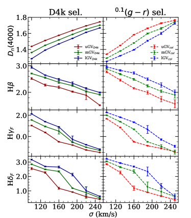
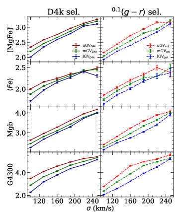
Figure 2: Comparison between line strengths of GV galaxies selected by 4000Å break strength (D4k) or dust-corrected ${}^{0.1}(g-r)$ colour (col). Each panel shows the results for the upper, middle and lower GVs, as labelled. Left: From top to bottom, we show the age-sensitive indices $D_{n}(4000)$, $H\beta$, $H\gamma_{F}$ and $H\delta_{F}$. Right: metallicity-sensitive indices (from top to bottom), [MgFe]^′, $\langle$Fe$\rangle$, Mgb, and the age-sensitive index G4300. All measurements are given as equivalent widths, in Å, except for $D_{n}(4000)$, which is a dimensionless ratio.

2.4 Uncertainty of the stacked spectra

One of the key constraints in our sample selection is the signal to noise ratio of individual spectra (snMedian_r$>$10) in order to avoid stacking large numbers of noisy data. This constraint results in stacked spectra with a very high S/N (see Fig. 1) when computed with the standard statistical noise carried from the individual data. Such high values of S/N lead to underestimated uncertainties on the derived parameters, as the higher values of the best-fit $\chi^{2}$ reflect the shortcomings of population synthesis models at this level of detail. Therefore to ensure our results have more realistic uncertainties, we adapt the noise level including two estimates – added in quadrature – that take into account additional sources of uncertainty in the stacking procedure. (1) We create Monte Carlo realisations of each stack by using the uncertainty of individual fluxes. We carry out the same analysis for these stacks as our original set, therefore giving us a more robust statistical uncertainty of the derived parameters. (2) For each velocity dispersion bin, we bootstrap the subsample, selecting, at random, only $60\%$ of the galaxies. We carry out the same process as for the original stacks, therefore incorporating the systematical uncertainty in our error bars caused by the sample selection. Bins comprising fewer galaxies are expected to carry a larger uncertainty, accounting for sample selection systematics.

Additional systematics may be expected, inherently to the methodology adopted here. One such systematic relates to the use of SSP models (Bruzual & Charlot, 2003; Vazdekis et al., 2012), that carry their own systematic uncertainties that depend upon the stellar library, isochrones and initial mass function (IMF) chosen. Furthermore, the use of STARLIGHT to perform spectral fitting will carry additional uncertainties. One way to mitigate this systematic would involve comparisons among independent spectral fitting algorithms, such as pPXF (Cappellari & Emsellem, 2004) or FIREFLY (Wilkinson et al., 2017), beyond the scope of this paper. Another source of uncertainty arises from the emission line correction that we apply to the Balmer absorption lines. However, our use of a battery of emission line diagnostics, and the comparison with spectral fitting – that mask out such regions – mitigates this potential systematic.

3 Line strength analysis

Our first approach to the analysis of the underlying stellar populations in GV galaxies focuses on the observed absorption line strengths. We select a battery of standard indices from the Lick system: $H\beta$, Mgb, Fe5270, Fe5335, G4300 (Trager et al., 1998), the higher order Balmer indices $H\gamma_{F}$ and $H\delta_{F}$ (Worthey & Ottaviani, 1997), as well as the $D_{n}(4000)$ (Balogh et al., 1999) index already used for the definition of the GV. We combine the iron abundance indices into an average $\langle$Fe$\rangle$ $\equiv$(Fe5270+Fe5335)/2, and also measure the standard index [MgFe]${}^{\prime}\equiv\sqrt{{\rm Mgb}(0.72\times{\rm Fe5270}+0.28\times{\rm Fe5335})}$ (Thomas et al., 2003). These indices can be split into two categories – age- and metallicity-sensitive. The Balmer indices, $D_{n}(4000)$ and G4300 are usually considered age-sensitive, while the others are metallicity-sensitive. However any and all spectral indices mentioned here (and, unfortunately, elsewhere) suffer from the age-metallicity degeneracy (e.g., Worthey, 1994; Ferreras et al., 1999).

3.1 General trends

This approach, solely based on the observed line strengths, is meant to assess in a model-independent way the variations between different regions across the GV. Fig. 2 shows the line strengths measured in the stacks, plotted with respect to velocity dispersion. We note these measurements are taken from the stacks that are smoothed to a common velocity dispersion of 235 km/s. Within each subfigure, the left (right) panels correspond to a selection of GV galaxies based on 4000Å break strength (dust-corrected ${}^{0.1}(g-r)$ colour). Each panel shows independently the trends in the upper, middle and lower GV, as labelled, including an error bar obtained from bootstrapping the sample. The $D_{n}(4000)$ index increases strongly with velocity dispersion in both cases and in all three regions of the GV, in agreement with previous studies (see, e.g., Kauffmann et al., 2003; Graves et al., 2009). However, at low velocity dispersion, the D4k selection produces overall higher values of the break, along with a wider range, towards lower values of the Balmer indices, consistently supporting the hypothesis that the D4k selection produces a GV with older and more homogeneous populations, especially at the low-mass end. At the high mass end, both selection criteria give rather similar results, although the lGV set defined by D4k appears to give slightly lower values than the colour-based lGV. However, this behaviour is not paralleled by the Balmer lines, so the mapping into population trends becomes less trivial. Nevertheless, the strong trends found in all age-sensitive indices with respect to velocity dispersion give robust confirmation of the well-known age-mass relation (see, e.g. Gallazzi et al., 2005).

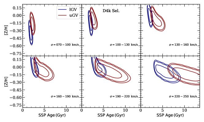
Figure 3: The likelihood derived from the line strength analysis of SSP-equivalent age and metallicity is shown with contour plots at the equivalent 1, 2 and 3 $\sigma$ levels. These stacks correspond to the selection of GV galaxies based on 4000Å break strength. The blue (red) contours represent lGV (uGV) stacks.

Both selection methods unsurprisingly produce the lowest (i.e. youngest) break strengths and highest (i.e. youngest) Balmer indices in the lGV at the low-mass end, whereas at high velocity dispersion, the differences between lGV and uGV are minor. We should keep in mind that the age-sensitive indices presented in Fig. 2 behave differently with respect to the age distribution, with the Balmer indices being more sensitive to recent star formation episodes compared to $D_{n}(4000)$ (Poggianti & Barbaro, 1997). Regardless of the GV selection method, as we traverse from lGV to uGV, we find a decrease in the line strengths of all Balmer indices, thus indicating a smooth transition from the younger lGV to the predominantly quenched, passively evolving uGV. It is worth noting that the colour-based selection produces overall higher Balmer indices, possibly implying the presence of younger (but dustier) galaxies, with respect to the D4k selection. Even though the colour selection includes an intrinsic dust correction, biases may appear as the correction is prone to systematics regarding the derivation of the dust corrections as well as variations of the dust attenuation law caused by the diverse range of dust geometry and chemical composition in galaxies (see, e.g. Tress et al., 2018; Narayanan et al., 2018). Moreover, note that the K-correction applied to bring the observed colour within a fiducial value (z=0.1 in our case) may also introduce an additional systematic: the median K-correction applied is 0.04 mag but there is an obvious dependence with redshift – with the correction trivially vanishing at z=0.1 – and a more subtle trend with the intrinsic colour – with the K-correction being larger in the redder galaxies. The difference in this correction with respect to the intrinsic colour can be as high as $\sim$0.1 mag, thus comparable with the interval that defines the GV. Such behaviour can introduce a correlation in the selection of the GV. In contrast, the 4000Å break selection depends neither on dust correction (see Appendix B) nor on the K-correction (as the index is directly measured on the rest-frame spectra).

The panels on the right of Fig. 2 present the results for metal-sensitive indices along with G4300. The index G4300 increases with velocity dispersion, roughly following a very similar trend as $D_{n}(4000)$. Note that this index separates more smoothly the lGV, mGV and uGV, confirming a strong correlation with the 4000Å break. For [MgFe]^′, $\langle$Fe$\rangle$ and Mgb, we find the expected positive correlation with increasing velocity dispersion (e.g., Sansom & Northeast, 2008). The line strength [MgFe]^′ – that can be approximately considered a total metallicity indicator – shows that, in general, the D4k selection features slightly more metal rich populations compared to the colour selection, in all GV regions. By comparing $\langle$Fe$\rangle$ and Mgb, we find both produce similar trends. As we move up the GV, from lGV to uGV, the data show increasing metallicity. It is worth mentioning here that the dependence of these indices on age – due to the age-metallicity degeneracy – is such that higher values of the index could also be explained by older ages. Section 4 is devoted to a comparison of the stacked spectra with population synthesis models via spectral fitting, to be able to break such degeneracies. Moreover, we show below (Section 3.2) an analysis of stellar ages based on simple stellar populations.

Therefore, Fig. 2 shows a subtle but measurable difference with respect to the GV selection method (D4k vs colour). These differences are especially substantial at low velocity dispersion, where the contribution from dusty, star-forming galaxies may introduce a larger systematic on the dust correction needed when using a colour selection.

3.2 Simple Stellar Population (SSP) properties

In A19 we provided an estimate of the SSP-equivalent ages of GV stacks restricted to the subset of quiescent galaxies. Here, we include star-forming and LINER-like AGN, to produce stacks that give a more comprehensive description of the average properties of GV galaxies. We also include more information about the SSP model fitting procedure – which is identical to the one presented in A19 – and extend the analysis, including a simple measurement of non-solar abundance ratios. The interpretation of the stacked spectra is done via a comparison of a selected set of age- and metallicity-sensitive line strengths, between the observed measurements and the values obtained from stellar population synthesis models.

3.2.1 Age and metallicity

In this section, we produce easy-to-interpret ‘SSP-equivalent’ ages, instead of a more complex combination of populations, left to Section 4. SSP-derived ages should be interpreted as a luminosity averaged age, as if the whole stellar content of the galaxy were formed in a single burst. An alternative definition – based on composite age distributions following a predefined functional form of the star formation rate – can be prone to biases due to the specific form adopted. We show both estimates of age in this paper to be able to assess the actual variations in the underlying populations of GV galaxies. We follow a Bayesian approach, probing a large volume of SSPs from the MIUSCAT population synthesis models (Vazdekis et al., 2012), comparing the observed and the model line strengths with a standard $\chi^{2}$ statistic:

$$\chi^{2}(t,Z)=\sum_{i}\left[\frac{\Delta_{i}(t,Z)}{\sigma_{i}}\right]^{2},$$ (6)

where $\Delta_{i}(t,Z)=O_{i}-M_{i}(t,Z)$ is the difference between the observed line strength and the model prediction for the $i$th index, and $\sigma_{i}$ is the corresponding uncertainty. The grid of SSP models comprise 8,192 synthetic spectra. The stellar age ranges from 0.1 to 13.5 Gyr, in 128 logarithmically-spaced steps, and metallicity ([Z/H]), varies from $-$2.0 to $+$0.2 dex, with 64 steps. We note the original models have a reduced set of metallicity steps (seven in total) and we interpolate (bi)linearly for a given choice of (log) age and metallicity.

Since the signal-to-noise ratio of the data is very high (Fig. 1), we need to apply offsets to the individual indices to account for potential variations due to differences in the [Mg/Fe] abundance ratio of the populations or, indeed, due to an extended age distribution. Our modus operandi involves computing the best fit solution (i.e. giving the minimum $\chi^{2}$) for a fiducial stack. This fiducial stack is chosen as the one that gives the lowest value of $\chi^{2}$ for the best fit. We then define the offsets for each line strength from this best fit solution, and apply these offsets ($\delta_{i}$), such that $\Delta_{i}(t,Z)=O_{i}-M_{i}(t,Z)-\delta_{i}$ in equation 6 – to all the stacks in the sample. Given the large S/N of the spectra, we also add in quadrature – as a potential systematic error, and in order to produce conservative error bars – an additional amount corresponding to 5% of the measured line strength. The resulting $\chi^{2}$ distributions are bivariate functions of age and metallicity. We fix the stellar initial mass function to Kroupa (2001). Note that the results for alternative choices of the IMF, such as Chabrier or Salpeter, give very similar results, and that, within the range of velocity dispersion values considered in this sample, no substantial variations of the IMF are expected (see, e.g. Ferreras et al., 2013).

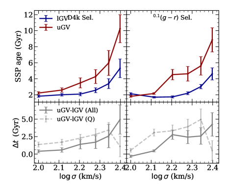
Figure 4: The SSP-equivalent age derived from line strengths is shown with respect to velocity dispersion in the lGV (blue) and uGV (red) subsets for the D4k- (left) and the colour-selected (right) GV. The bottom panels show the age difference between uGV and lGV stacks. These are derived from the stacks presented in this paper, that comprise quiescent, star-forming and LINER AGN galaxies. The dashed grey lines in the bottom panels contrast the results with A19, where the stacks only involve quiescent GV galaxies.

Fig. 3 shows the corresponding probability contours of the bivariate likelihood ${\cal P}(t,Z)$ derived from the spectral stacks of the uGV (red) and lGV (blue) galaxies, selected according to 4,000Å break strength. The contours are slightly smoothed by a Gaussian kernel, and shown at the equivalent 1, 2 and 3 $\sigma$ confidence levels, with each panel representing a velocity dispersion bin. Note the expected positive correlation between velocity dispersion and either SSP-equivalent age or metallicity. We note that the method is especially good for determining relative variations in the stellar age, whereas metallicity is less well constrained. The difference in age between lGV and uGV galaxies is apparent. We marginalize over metallicity, producing the trends in SSP-equivalent age shown in Fig. 4, with the error bars given at the 1 $\sigma$ level. We show the uGV and lGV trends with respect to velocity dispersion in the D4k-selected (left) and colour-selected (right) GV. The bottom panels show the age difference between the two. We stress that this paper focuses on spectral stacks that include star-forming, quiescent and LINER-like galaxies. The dashed grey lines in the bottom panels show the analysis when restricting the stacks to quiescent galaxies, as shown in fig. 4 of A19. Both sets of stacks feature a similar increasing trend with $\sigma$, except at the highest velocity dispersion bin, where the quiescent sample shows a significant decrease.

3.2.2 [Mg/Fe]

Overabundances in [Mg/Fe] are traditionally associated with short and intense star formation episodes where the delayed Fe-rich contribution from type Ia supernovae is not incorporated into stars (see, e.g., Thomas et al., 1999). Standard models based on a single or double degenerate progenitor imply delays between 0.5 and 2 Gyr (Matteucci & Recchi, 2001). Therefore, populations with super-solar [Mg/Fe] are expected to have been formed over similar timescales. Therefore, an estimate of [Mg/Fe] provides a stellar clock that has been exploited, for instance, to show that massive early-type galaxies must have formed their central regions within a dynamical timescale. Here we look for potential variations of [Mg/Fe] in the stacked GV spectra, following the proxy adopted in La Barbera et al. (2013). This proxy allows one to use standard, solar-scaled population synthesis models to measure [Mg/Fe]. The procedure involves constraining a grid of SSP models using two different sets of line strengths, one involving age-sensitive indices along with an Mg-sensitive index (obtaining a metallicity [Z_Mg/H]; in this case we use Mgb) and another one involving the same age-sensitive indices plus a Fe-sensitive index (producing [Z_Mg/H], we use here $\langle$Fe$\rangle$). The difference, i.e. [Z_Mg/Z_Fe] is the adopted proxy for [Mg/Fe].

Fig. 5 plots [Z_Mg/Z_Fe] against velocity dispersion for both definitions of the GV, where the numbers in the legend represent the Pearson correlation coefficient (pcc). Our estimate of pcc along with its uncertainty involves 100 Monte Carlo realisations. For each realisation, we remove at random one data point and calculate the resulting pcc; this is done to mitigate the effect of outliers. The pcc is quoted as the median of the distribution and the uncertainty is one standard deviation. The data points are shifted horizontally by an arbitrary amount to avoid overcrowding. In the D4k selection (top panel), the uGV behaves differently with respect to lGV and mGV, which behave in a similar manner to each other. Both mGV (pcc=$+0.77\pm 0.06$) and lGV (pcc=$+0.59\pm 0.14$) show a weak but significant correlation with velocity dispersion, whereas the abundance ratio in uGV galaxies (pcc=$-0.24\pm 0.14$) seems rather constant. Interestingly, the colour-based selection (bottom panel) shows an increasing trend in all subsamples of the GV, although [Z_Mg/Z_Fe] appears to flatten in uGV galaxies with $\sigma\gtrsim$150 km/s. The trends support the scenario of a more extended star formation history in lower mass galaxies (see, e.g., de la Rosa et al., 2011).

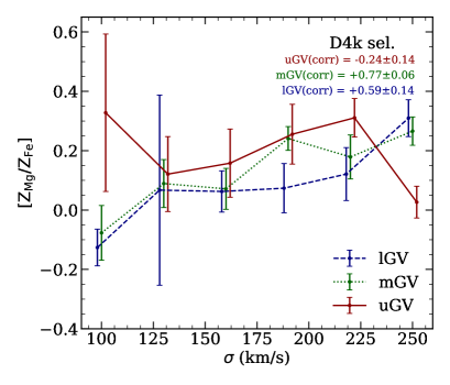
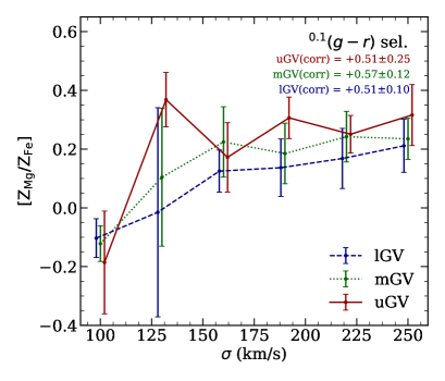
Figure 5: The relation between the abundance ratio proxy $\mathrm{[Z_{Mg}/Z_{Fe}]}$ and velocity dispersion for 4000Å break strength (top) and colour selection (bottom). The blue, green and red lines show the trends for lGV, mGV and uGV galaxies, respectively (see text for details about the derivation of this [Mg/Fe] proxy). The numbers in red, green, and blue show the Pearson correlation coefficient (pcc) between $\mathrm{[Z_{Mg}/Z_{Fe}]}$ and velocity dispersion in the uGV, mGV and lGV subsamples, respectively.

3.3 Difference regarding (nebular) activity

In A19, we restricted the stacking procedure to quiescent galaxies. The motivation in that letter was to assess the transition period of quenched galaxies across the GV, by considering systems where star formation is already absent. In this paper, we consider, instead, the general trends of GV galaxies, so that the different contributions of quiescent, star-forming, and AGN systems (see Table 1) manifests in those trends. Moreover, as systems with nebular emission are expected to be significantly affected by dust, we want to explore the differences between the D4k selection (minimally affected by dust) and the colour selection (that applies a dust correction, but may be affected by systematics from this correction). Therefore, a comparison between the quiescent stacks of A19 and those that include star forming and LINER-like emission, provides useful insight on the properties of GV galaxies and the potential biases caused by the selection method.

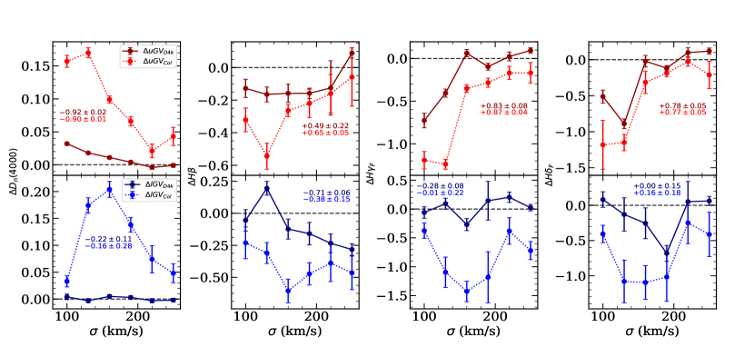
Figure 6: Differences in age-sensitive line strengths between uGV (top panel) and lGV (bottom panel) between Q only stacks and “full” stacks, comprising SF, LINERS and Q galaxies. The light red and blue dotted data shows the difference for colour selection, while dark red and blue solid lines show the difference in the D4k selection. Likewise, the numbers shown in light red and light blue give the Pearson correlation coefficient regarding the colour selection data points, while the dark red and blue text shows the correlation coefficient calculated for the D4k-selected sample. The error bars are quoted at the 1 $\sigma$ level.

Fig. 6 shows the difference in the age-sensitive indices between the Q stacks (hereafter $Q_{stack}$) and the combined Q$+$SF$+$LINER stacks (hereafter $All_{Stack}$). The top and bottom panels show the difference in results for uGV and lGV galaxies, respectively. Solid and dashed lines show the results for D4k and colour selection, respectively. In uGV galaxies, a decrease in the difference of $D_{n}(4000)$ with respect to velocity dispersion is evident, for both D4k (pcc=$-0.92\pm 0.02$) and colour selection (pcc=$-0.90\pm 0.01$). This trend can be attributed to the lower contribution of star-forming galaxies as velocity dispersion increases (see Table 1). It should be noted that the variation in $\Delta D_{n}(4000)$ (leftmost panels) for the D4k selection should be, by construction, minimal, as we are constraining the $D_{n}(4000)$ index within certain values. Note, in contrast, the different trends found in the Balmer indices. For the uGV, inclusion of SF galaxies increases Balmer absorption in both definitions of the GV, as expected from the decrease in average age. Furthermore, the values of pcc show a stronger correlation/anti-correlation in uGV in comparison to lGV; this effect can be attributed to a lower percentage of SF and AGN galaxies in uGV in contrast to lGV with increasing velocity dispersion. We find a more homogeneous distribution of stellar populations when GV galaxies are selected according to D4k, whereas the colour-based selection produces larger differences in the indices in both uGV and lGV.

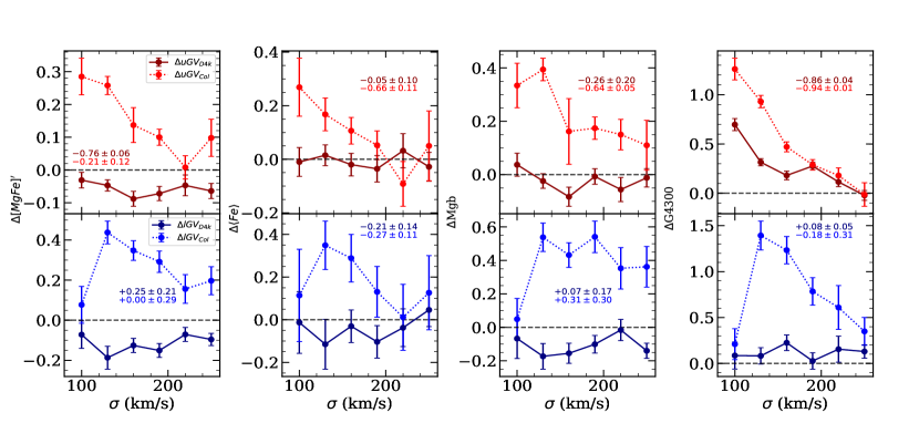
Figure 7: Same as Fig. 6 but here we show metallicity sensitive indices and G4300.

Fig. 7 shows the results for the remaining line strengths. Note the age-sensitive G4300 behaves similarly to $D_{n}(4000)$, as in Fig. 2. Both Figs. 6 and 7 show that in all cases, the line strength variations are significantly smaller for the D4k selection, confirming that a more homogeneous distribution of GV galaxies is produced when selecting the sample on break strength. A colour-based selection, even after a careful dust correction is applied, produces a more complex mixture of galaxies, regarding nebular activity. We argue that the D4k selection results in a more representative sample of transitioning galaxies from the BC to the RS. Note that for the metallicity sensitive indices, the difference between stacks gives a negative value, that may suggest lower average metallicities when stacking only quiescent galaxies. Note that, e.g. [MgFe]^′ also increases with stellar age, so that an age-dependent explanation would need to invoke younger populations in Q galaxies. In contrast, the colour selection yields positive variations in the metal-sensitive indices, as expected if $All_{stack}$ is dominated by younger, metal-poor, star-forming galaxies. This result further supports the idea of population contamination when using colour selection. This contamination seems to affect not only the age- but also the metallicity-sensitive indices at all values of the velocity dispersion, although the difference appears to decrease towards higher velocity dispersion, where the contamination from dusty BC galaxies decreases.

4 Spectral fitting analysis

In order to look in more detail at the stellar population content of GV galaxies, we carried out spectral fitting, by use of the STARLIGHT code (Cid Fernandes et al., 2005), to produce best-fit composite mixtures. Variations of these mixtures across the GV will inform us of the transition between the lGV to the uGV – note that depending on whether the dominant mode is quenching or rejuvenation, it is possible to evolve in both directions. STARLIGHT performs linear superpositions of simple stellar population (SSP) spectra supplied by the user, selecting a best fit by minimizing a $\chi^{2}$ statistic with an MCMC sampler. In this paper we use a grid of $N_{*}$=138 SSPs from the models of Bruzual & Charlot (2003, hereafter BC03), adopting a Chabrier (2003) IMF. Our grid consists of 28 distinct stellar ages and 6 different metallicities. The age ranges from 1 Myr to 13 Gyr, spaced logarithmically, and the metallicity varies from [Z/H]=$-$2.3 to $+$0.4.

We mask out the standard spectral regions where nebular emission may be prominent. The fitting range we chose – 3500-7500Å– includes a number of age- and metallicity-sensitive regions such as those targeted in the previous section. Spectral fitting provides an alternative approach to individual line strength analysis; the larger amount of information, including the stellar continuum from the NUV, optical and NIR windows, allows for constraints on more complex distributions of stellar ages and metallicities.

4.1 Luminosity-weighted parameters

Fig. 8 shows the luminosity-weighted averages of some key stellar population parameters of the GV stacks as a function of velocity dispersion. The left (right) panels show the D4k- (colour-) based selection, respectively. The blue dashed, green dotted and red solid lines represent the result for lGV, mGV and uGV, respectively. Each panel quotes the corresponding Pearson correlation coefficient (pcc). From top to bottom, we show the average stellar age, $\langle t\rangle$, a parameter, $\Delta t$, defined below, that keeps track of the width of the age distribution, the average total metallicity, $\langle[Z/H]\rangle$, and the dust attenuation applied as a foreground screen, $A_{V}$. The average age is defined as:

$$\langle\log\ t\rangle=\sum_{j=1}^{N_{*}}x_{j}\,\log\ t_{j},$$ (7)

where $x_{j}$ is the normalized luminosity weight (i.e. $\sum_{j}x_{j}=1$) and $t_{j}$ is the age of the $j$-th SSP in the basis set (see Cid Fernandes et al., 2005, for details). The average age shows the well-established trend, where velocity dispersion, roughly a proxy for galaxy mass, is positively correlated with the average age (e.g., Gallazzi et al., 2005). Galaxies on the uGV are consistently older at all values of velocity dispersion. The age difference between mGV and lGV is less prominent than between these two and the uGV. A possible explanation for this trend is discussed in Sec. 5.2. The age difference between the uGV and lGV stays in the region 0.5-1 Gyr, a consistent result with respect to the SSP analysis shown in Sec. 3.2.

The uncertainties of the parameter estimates are obtained by making 20 Monte Carlo realizations of each stack, by adding noise consistently with the uncertainties in each flux bin, and re-running each one of them through STARLIGHT. The realizations produce a distribution from which the standard deviation of the parameter estimates is quoted as the uncertainty. Galaxies in the lGV have a smoother age trend with respect to velocity dispersion.

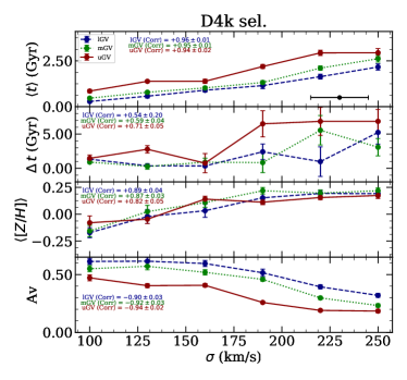
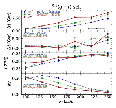
Figure 8: From top to bottom, trends with velocity dispersion of average stellar age, $\Delta t$ – that acts as pseudo quenching timescale – metallicity, and dust attenuation. The blue dashed, green dotted and red solid lines show the results for lGV, mGV and uGV, respectively. Results are shown for the 4000 Å  break selection (left) and the colour selection (right) of GV galaxies. The numbers in each panel quote the Pearson correlation coefficient (pcc), where the colours correspond to lGV, mGV and uGV, accordingly.

The second age indicator, $\Delta t$ (second panel from the top), is extracted from the cumulative stellar mass profile:

$${\cal C}(s)=\sum_{j}x_{j}(t\leq s).$$ (8)

Defining the inverse of this function as $\tau(y)\equiv{\cal C}^{-1}(y)$, we take the time interval $\Delta t\equiv\tau(0.70)-\tau(0.30)$, i.e. the time lapse spanning the epochs when the galaxy, or its progenitors, formed between 30% and 70% of its total stellar mass. The motivation behind this definition is to provide a GV transition interval that could be related, for instance, with a quenching timescale. However note two important caveats. Firstly, if the galaxy has experienced a rejuvenation episode, the recently formed stars will be given more weight, thus leading to high $\Delta t$ values: even if the actual quenching timescale is relatively short. Secondly, we are dealing with stacks that include star-forming galaxies. Therefore, our definition of $\Delta t$ should be considered as an effective GV timescale, rather than a true quenching interval. Previous results from the literature noted that the quenching timescale evolves in a complex way with velocity dispersion, with an initial increase, followed by a decrease at the massive end (Gabor et al., 2010; Wright et al., 2019). Here, we find $\Delta t$ increases in all cases, in contrast with the trends found in the line strength analysis of A19, where a non-monotonic behaviour was found between the SSP-equivalent age difference of galaxies on the uGV and lGV with respect to velocity dispersion.

The third panel from the top shows the average total metallicity, calculated in a similar manner to average age, namely:

$$\langle[Z/H]\rangle=\sum_{j=1}^{N_{*}}x_{j}[Z/H]_{j},$$ (9)

where $[Z/H]_{j}$ is the individual SSP metallicity of the $j$th component. A strong positive trend is also found between total metallicity and velocity dispersion, once more in agreement with previous studies of the general population (see, e.g., Gallazzi et al., 2005; Graves et al., 2010). At the low mass end, the colour-based selection (panels on the right), shows a consistent trend towards a higher metallicity in the uGV with respect to the lGV. However, this trend is less evident in the D4k selection (left panels), which is less sensitive to contamination from dusty, star-forming (and possibly lower metallicity) galaxies, especially in the lGV; resulting in a weaker correlation for D4k selected samples in comparison to a colour-based GV. The D4k selection shows that, within error bars, metallicity does not segregate within the GV at fixed velocity dispersion. This result suggests a potential bias when selecting GV according to colour. The next (bottom) panels of Fig. 8 show the monotonically decreasing trend of dust attenuation with $\sigma$, consistent with previous studies (e.g., La Barbera et al., 2014), featuring a clear stratification from lGV to uGV, with mGV galaxies having, once more, properties closer to lGV galaxies. This information can also help assess potential biases related to the dust correction needed in the colour-based selection. It is worth mentioning the small difference in $A_{V}$ at the lowest velocity dispersion in colour-based GV galaxies. One could argue that the dust correction could be partly responsible for this result, whereas the D4k selection shows the $A_{V}$ stratification between uGV, mGV and lGV at all values of $\sigma$.

Fig. 9 shows the variation in average metallicity as a function of $\Delta t$ and average age, as labelled. The results of a D4k (colour) selection of GV galaxies is shown on the left (right) panels, following the same colour coding as the previous figure to represent the uGV, mGV, lGV stacks. The marker size maps velocity dispersion. Focusing on the D4k selected sets, we find two different trends in the sample: i) At low metallicity ($\langle[Z/H]\rangle\lesssim+0.1$), GV galaxies have short $\Delta t\,\,(\lesssim$3 Gyr); ii) At higher metallicity, GV galaxies have a broader distribution of $\Delta t$, a result indicative of rejuvenation. In this region, galaxies have higher velocity dispersion and feature older stellar populations. Moreover, lGV and mGV galaxies have relatively shorter $\Delta t$, with respect to uGV systems, that have $\Delta t\gtrsim$5 Gyr. Therefore, a higher fraction of uGV galaxies at the massive end appear to have undergone more substantial episodes of rejuvenation. The standard age-metallicity relation can be found in the figure, with a significant stratification towards older populations at fixed metallicity in uGV galaxies. This effect is more pronounced in the D4k selection, whereas the colour-based selection produces a more complex mixture at low velocity dispersion, as expected from the contribution of dust, more prevalent at this end of the distribution.

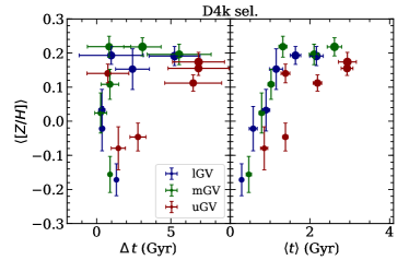
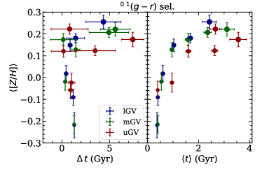
Figure 9: Trends between metallicity and either $\Delta t$, or average age. The blue, green and red data points show the results for lGV, mGV and uGV respectively. The marker size follows velocity dispersion. The uncertainty in average metallicity remains constant, whereas the error bar in $\Delta t_{Q}$ increases with average metallicity. Results are shown for the 4000 Å break selection (left) and the colour selection (right) of GV galaxies.

4.2 Star Formation History (SFH)

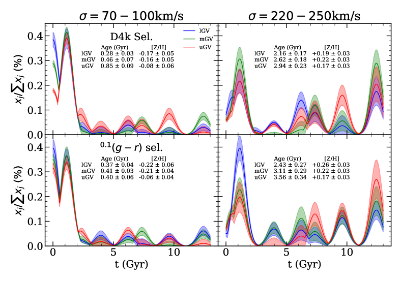
Figure 10: The star formation history is shown for both $D_{n}(4000)$ (top) and colour (bottom) selected GV galaxies. The left and right sides show the SFH in the lowest velocity dispersion bin $70<\sigma<100\,$km/s and the highest velocity dispersion bin $220<\sigma<250\,$km/s, respectively. The blue, green and red curves represent the SFHs of lGV, mGV and uGV galaxies, respectively.

The next step in the analysis of the spectral fitting constraints is the star formation history, namely the distribution of SSP weights, ${x_{j}}$ as a function of age – i.e. marginalized with respect to metallicity. Note that individual SFHs constrained on a galaxy by galaxy basis are rather uncertain with any population fitting code, and STARLIGHT is no exception. However as we are dealing with stacked spectra covering a large number of galaxies, we can assume that the derived SFHs represent statistical trends in the various regions of the GV probed here. Fig. 10 shows the luminosity-weighted output for lGV (blue), mGV (green) and uGV (red). The histograms bin the age intervals in a linear manner. The average age and metallicity, quoted in each panel, have been calculated using the SSP ages of the basis set, along with their corresponding weights, following equations 7 and 9. The left and right panels show the results at the lowest and highest velocity dispersion bins, 70$<\sigma<$100 km/s and 220$<\sigma<$250 km/s, respectively. The upper (lower) panels show the results for the D4k (colour) selection, as labelled. Note these results are robust regarding the relative weight contributions, whereas absolute estimates may carry larger uncertainties. To assess the statistical uncertainty, we perform for each stack a Monte Carlo set of 20 realizations of spectra with the same flux distribution and noise compatible with the stack under consideration, following an identical methodology. The shaded regions in the figure show the expected uncertainty from this comparison. Note that spectral fitting inherently constrains luminosity-weighted properties. A translation into mass-weighted values unavoidably carries additional uncertainties, related to the mapping from luminosity into stellar mass. For instance, a recent episode of star formation can bias the results as the hot, massive stars present in young populations contribute significantly more than their cool, low-mass (although equally young) counterparts.

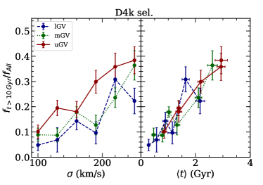
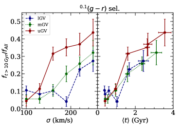
Figure 11: Relation between the mass fraction in old stellar populations ($\gtrsim$10,Gyr), with respect to velocity dispersion (left) and average age (right). The blue, green and red lines correspond to lGV, mGV and uGV galaxies, respectively. Results are shown for the 4000 Å break selection (left) and the colour selection (right) of GV galaxies.

At low velocity dispersion (left panels) the stellar populations are mostly young. As we traverse the GV from lGV to uGV, more weight is given to the older components, increasing the average age from $\langle t\rangle\sim$0.3 Gyr in the lGV to $\sim$1 Gyr in the uGV, for the D4k selection, whereas the colour-based selection produces a more homogeneous distribution, with undistinguishable age differences “across the valley”, and a significantly larger scatter. In all cases, the SFHs concentrate within the most recent $\sim$2 Gyr, with small, subdominant old populations that become, only slightly, more prominent in the uGV. At high velocity dispersion (right panels), the SFHs evolve towards older components, with average (luminosity-weighted) ages $\sim 2-3$ Gyr.

Fig. 11 shows the variation of the mass fraction in old ($>$10 Gyr) stars with respect to velocity dispersion and average age, for the D4k (left) and colour (right) selection. Both cases produce similar increasing trends of the old contribution in the most massive galaxies and towards higher average ages. The latter statement is not trivial, as this diagnostic is sensitive to whether the age distribution changes its width with respect to average age. The D4k selection produces consistently higher old stellar fractions at all values of velocity dispersion, whereas the colour-based selection, once more, shows some mixing at the low mass end. Regardless of the selection process, uGV galaxies display more of a difference with respect to mGV and lGV galaxies. Note that at low velocity dispersion, the colour selection yields a lower fraction in old stars, specially in the uGV. This is interesting as even though both selection methods feature not too dissimilar low fractions of Q galaxies ($7.3\pm 0.4$% for D4k, and $4.2\pm 0.4$% for colour), we see a greater number of SF galaxies in the colour-based selection (namely $70.0\pm 1.3$% in the D4k selection versus $78.4\pm 2.1$% for the colour selection). This could be a further indication of a possible bias due to dust attenuation that causes BC galaxies to “creep” into the GV (Schawinski et al., 2014). This theory is further supported at intermediate velocity dispersion bins, 100$<\sigma<$190 km/s, where even though there is a lower contribution of SF galaxies in the D4k Selection of the uGV, a higher fraction of old stars is found in the colour-based GV stacks.

4.3 Mass-weighted population properties

In addition to the luminosity-weighted properties presented above, we can extend the analysis by use of the stellar mass to light ratio ($\Upsilon_{\star}$) provided by the population synthesis models for each SSP. Although this translation carries additional uncertainty, it is a way to assess whether the older components are more dominant than expected from a simple fit to the observations, which are inherently biased towards the most luminous stars. Mass-weighted parameters provide a more physical interpretation of the SFHs. The analysis is based on models with a fixed initial mass function, namely Chabrier (2003). We stress that within the velocity dispersion probed by this sample, no significant variations from a “standard” IMF are expected (see, e.g., Ferreras et al., 2013; La Barbera et al., 2013).

Fig. 12 is the equivalent of the best-fit stellar parameters shown in Fig. 8 for the mass-weighted case, using the same line and colour coding. Similarly to the luminosity-weighted values, a general increase is found in average age with velocity dispersion but the absolute values are higher, as expected, and plateau at the massive end. Regarding GV sub regions, we also find here more affinity between lGV and mGV, whereas uGV galaxies appear older. This result is consistent regardless of the GV selection method, confirming that a selection based on the 4000Å break provides a homogeneous population. An increased scatter is evident in the mass-weighted estimates, partly due to the added uncertainties regarding the translation from light to mass. The $\Delta t$ parameter shows a significant difference with respect to the luminosity-weighted counterpart, with overall high values and a decreasing trend with velocity dispersion, and no segregation regarding GV location (i.e. lGV, mGV and uGV). Note, though, there is an anti-correlation, that is weaker in comparison to Fig. 8. Estimates of average metallicity are now higher, and appear rather flat with respect to velocity dispersion, within error bars.

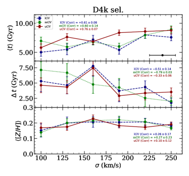
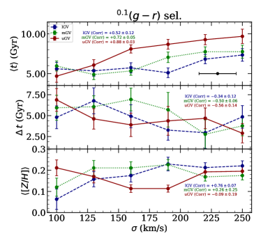
Figure 12: This is the equivalent of Fig. 8, showing mass-weighted parameters.

5 Discussion

This paper looks in detail at the stellar population properties of green valley galaxies, selected with a new methodology based on the 4000Å break strength (A19), and contrasts the results with respect to the traditional approach based on dust-corrected broadband colours. In this section we briefly explore the implications of this analysis.

5.1 Dust-related systematics

The traditional selection of GV galaxies, based on colours derived from broadband photometry, is affected by dust attenuation. In order to remove the effect of dust, a model is applied to derive a colour correction term. However, these corrections are subject to uncertainties that depend on the model fitting as well as on additional systematics related to the details of dust attenuation in galaxies. It is worth emphasizing that the net effect of dust is to impose an effective, wavelength-dependent attenuation law. However, in detail, it is a result of a wide range of mechanisms involving scattering and absorption of photons from the illuminating source (i.e. the underlying stellar populations) by the dust particles. The effective attenuation depends not only on the composition of dust, but also on its distribution within the galaxy (see, e.g., Galliano et al., 2018). The dust is typically concentrated around star-forming sites, and motivates the birth cloud model, where a time-dependent dust attenuation provides a suitable description of the net attenuation law (see, e.g., Charlot & Fall, 2000). Observationally, star-forming galaxies feature a wide range of effective attenuation laws beyond the standard ones that fit the Milky Way average extinction curve (Cardelli et al., 1989) or the average attenuation of star-burst galaxies (Calzetti et al., 2000). The variation of the parameters that describe the attenuation law also appear to correlate (Tress et al., 2018; Narayanan et al., 2018). Therefore, such trends can lead to significant systematics in the dust correction.

Our comparison of GV galaxies between the dust-corrected colour selection and our proposed 4000Å break strength selection enables us to assess the role of these systematics. In appendix B we quantify the dependence of the two observables chosen to select GV galaxies, on dust attenuation, using a simple attenuation law parameterised by the colour excess.

Table 1, in the appendix, shows the fraction of galaxies in the lGV and uGV, when selected according to either D4k or colour, with the latter shown with and without a dust correction. A graphical description of this table can be found in fig. 3 of A19. Note the D4k-selected GV yields a larger population of SF galaxies, than the uncorrected colour selection, especially towards high velocity dispersion ($\sigma\sim$200 km/s), along with a lower percentage of Q galaxies. Such a trend could be down to 2 reasons. Firstly, dust could have reddened the galaxies to different amounts, so that SF galaxies occupy a wider region, leading to broader Gaussian PDFs when performing a colour-based selection. Secondly, due to our GV definition being dependent on the PDF of SF galaxies, the GV might have been shifted towards the RS in the colour-based approach. This explains the large (small) percentage of Qs (SF) population in lGV $72.5\pm 13.5\%$ ($7.5\pm 4.3\%$)and uGV $82.2\pm 13.5\%$ ($8.9\pm 4.4\%$), at the highest velocity dispersion ($220<\sigma<250\,$km/s).

The introduction of a dust correction makes the D4k- and colour-based selections closer together (see also fig. 3 of A19), illustrating the importance of dust correction when using colours. In more detail, note that the dust-corrected colour-based GV gives a lower fraction of Q galaxies in both lGV and uGV, with respect to the D4k selection. Although this might seem counter-intuitive, note that the largest effect when applying the dust correction of the colours is to increase the number of SF galaxies. Therefore, we deduce that most of the galaxies that appear on the GV after the dust correction is applied originate from the RS defined by the dust-uncorrected classification – as the effect of the correction is always to make the colours bluer. Another interesting trend can be seen when going from intermediate ($\sigma$=160–190 km/s), to high ($\sigma$=190-220 km/s) velocity dispersion, where we see an increase in the SF population in both D4k and dust-corrected ${}^{0.1}(g-r)$ selection of lGV and uGV. Note this trend is not seen in the dust uncorrected ${}^{0.1}(g-r)$ selection.

Moreover, note the difference in the line strengths between the full GV stacks and those consisting exclusively of Q galaxies – shown in Figs. 6 and 7. The D4k-selected sample shows a more homogeneous distribution, in contrast with the larger variations found in the colour-based selection. These results illustrate the highly non-trivial issue of the systematics expected in the selection of GV galaxies, and leads us to adopt the D4k selection as a more robust representation of the GV.

5.2 Interpretation of the GV as a transition region

We now take the D4k-selected GV as our standard sample. The differences in the stellar population properties of the three different areas of the GV, at fixed velocity dispersion, reflect the nature of the GV as a transition phase. The line strength results allow us to see in a model-independent way these variations. Fig. 2 shows a substantial difference in the higher order Balmer lines, especially H$\delta_{F}$, with respect to the other indices. This line is especially sensitive to recent episodes of star formation (see, e.g., Martin et al., 2007) and thus may imply, when considering stacked spectra, that the contribution from rejuvenated galaxies dominates the flux, especially at high velocity dispersion. Also note that at low velocity dispersion, the trend of H$\delta_{F}$ is smoother, tentatively meaning that a smoother decaying (or truncated) star formation is in operation, suggesting a quenching mechanism – of otherwise younger populations – at the low-mass end.

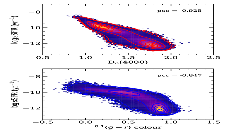
Figure 13: Relation between the sSFR and D4k $({\it top})$ and sSFR and dust-corrected colour $({\it bottom})$. The values denoted by pcc give the Pearson correlation coefficient. Note D4k shows a stronger (anti-)correlation with sSFR than colour.

Further supporting the results from line strength analysis, the population constraints based on spectral fitting (Fig. 8), give further evidence towards rejuvenation at high velocity dispersion: the parameter $\Delta t$ is defined as an estimator of the width of the stellar age distribution, and stays at $\Delta t\lesssim$2 Gyr for $\sigma<$170 km/s (luminosity-weighted) – corresponding to a more compact age distribution – followed by very large values of $\Delta t$ at the massive end, as expected from the presence of two or more disjoint star formation events across cosmic time, expected when rejuvenation produces a significant young component. Moreover, Fig. 11 emphasizes that the fraction of old ($>$10 Gyr) stars in uGV galaxies is high in massive galaxies and low at small velocity dispersion. Therefore, in this SDSS-based, low-redshift sample, quenching appears at late cosmic times in low-mass galaxies, whereas at the massive end one can only measure recent rejuvenation events on an otherwise old population. The mass-weighted results (Fig. 12) feature more scatter – as expected from the added uncertainties in $\Upsilon_{\star}$,when converting the SSP contributions into mass fractions – but interestingly produce a decreasing trend of $\Delta t$ with velocity dispersion, implying that the rejuvenation events at the massive end cannot involve a large mass fraction of young stars. Nelson et al. (2018) explored the fractional contribution of rejuvenated galaxies in the IllustrisTNG simulation, finding that $\sim 10\%$ of the subset of massive galaxies (M${}_{\star}/\mathrm{M_{\odot}}>10^{11}\mathrm{M_{\odot}}$) have undergone rejuvenation once and $\sim 1\%$ have experienced more than one rejuvenation event. Note our analysis shows rejuvenation to be dominant in stacked spectra at the massive end. However, the percentage of different types of galaxies in the stacks (Tab. 1) are roughly in agreement with the numerical simulations. Focusing on the uGV at high velocity dispersion (220$<$$\sigma$$<$250 km/s) we find 19% are star-forming galaxies. If we assume that a fraction of these SF galaxies are simply transitioning from BC to RS, with the remainder representing rejuvenation events, i.e. galaxies that have dropped down from RS, we might find similar fractions of rejuvenated systems as those found in the literature (Thomas et al., 2010; Nelson et al., 2018). A similar argument can be made for galaxies in lGV and mGV. However, the fractional contribution from star-forming galaxies is higher, and we expect a smaller contribution from rejuvenation events.

Regarding metallicity, we recover the standard mass-metallicity relation, as shown in Fig. 8. Although on a speculative tone, note the metallicity trend between uGV and lGV gets inverted between low- and high velocity dispersion (in the luminosity weighted version). Such a trend would be a consequence of fresh, lower metallicity gas contributing to the rejuvenation events at the massive end of the sample.

Concerning the transition from BC to RS, previous work from the literature indicates a rapid evolution through the GV due to its sparsity (see, e.g., Baldry et al., 2004; Taylor et al., 2015). However, this transition time depends on morphology. For instance, Schawinski et al. (2014) distinguish at least two morphologically-related transition paths. Early-type galaxies are thought to traverse the GV in a rapid manner, quenching their star formation very quickly and moving onto the RS, while, in contrast, late-type galaxies are expected to undergo a slower quenching process. This is supported by Kelvin et al. (2018), where they look at structural variations with respect to colour and morphology, and argue in favour of inside-out formation, which is related to slow quenching, instead of a violent transformative event. Additionally, the observational constraints from the stacked spectra give timescales between 2 to 4 Gyr (Phillipps et al., 2019). Using SSP-equivalent ages, the derived transition times are similar when stacking spectra regardless of nebular activity (Fig. 4). However, the difference between uGV and lGV luminosity-weighted average ages, from spectral fitting, results in a lower transition time $\sim$1.0 Gyr. Interpreting $\Delta t$ as a transition timescale leads to a higher value $\gtrsim$5 Gyr, with respect to Phillipps et al. (2019). Note this is to be expected as (i) STARLIGHT is very robust at tracing average parameters but produce weaker constraints on the details of the SFH; (ii) The parameter $\Delta t$ traces the transition time in a slightly different manner, as it is very sensitive to recent bursting episodes (see Sec. 4.1 for details), while the methodology adopted by Phillipps et al. (2019) uses a fixed exponentially decaying SFH, thus making it less sensitive to rejuvenation effects.

In addition, state of the art simulations give further support to a rapid transition through the GV; Wright et al. (2019) state that low velocity dispersion galaxies feature relatively long quenching timescales, $\tau_{Q}\gtrsim$3 Gyr. This timescale increases with velocity dispersion; but at the highest values of velocity dispersion, they find a drop to $\tau_{Q}\lesssim$2 Gyr. As for the physical mechanism that produces this transition, it is stated that in low-mass galaxies it is mostly due to processes such as ram pressure stripping, while in more massive galaxies quenching operates though events such as stellar feedback (Wright et al., 2019). Finally, in the most massive systems, major mergers and quasar-mode AGN are thought to quench star formation.

Finally note the similar behaviour between lGV and mGV, in contrast with uGV for the D4k-selected sample. Interestingly, this behaviour between the different GV regions was also seen by Phillipps et al. (2019) in their study of “green” galaxies using sSFR. They noted a lower transition time going from their “lGV” to “mGV” – selected by sSFR_lGV/sSFR${}_{mGV}\sim$1.6, giving 2 Gyr – with respect to their “mGV” to “uGV” – selected by sSFR_mGV/sSFR${}_{uGV}\sim$ 2.5, giving 3–4 Gyr. Fig. 13 shows the relation between D4k and sSFR $({\it top})$ and between colour and sSFR $({\it bottom})$. The relation with D4k presents a stronger correlation (pcc=$-$0.925) compared to colour (pcc=$-$0.847), therefore it is not surprising that sSFR behaves in a similar manner to the 4000Å break strength. This similarity reinforces the trends found here.

6 Conclusions

We present in this paper a detailed analysis of the recently proposed re-definition of green valley galaxies based on the 4000Å break strength (A19), along with a comparison with the standard selection based on dust-corrected colours from broadband photometry. We make use of a large sample of high quality spectroscopic data from the Sloan Digital Sky Survey (SDSS). The new definition adopts the well-known spectral index D_n(4000) of Balogh et al. (1999), whereas the colour-based approach uses the SDSS-defined, dust corrected colour ${}^{0.1}(g-r)$, i.e. K-corrected to redshift z=0.1. The “population” indicator, i.e. either D_n(4000) or ${}^{0.1}(g-r)$, is plotted against velocity dispersion ($\sigma$), and the sample – defined between 70 and 250 km/s – is split into six bins in $\sigma$. A probability-based approach is followed, where the star-forming and quiescent samples define a Blue Cloud (BC) and a Red Sequence (RS), respectively, and an intermediate population, i.e., the green valley (GV) is introduced, and further split into three regions, lower (lGV), middle (mGV) and upper (uGV), based on the value of the population indicator.

Our results show overall consistent properties between the new definition, that is more resilient to potential systematics from the dust properties, and the dust corrected selection based on colour, with similar fractions between star-forming (SF), quiescent (Q) and AGN galaxies, with respect to velocity dispersion (see Table 1 and fig. 3 in A19). However, when studying the stellar population property in more detail, differences are found between these two selection criteria that may affect the interpretation of galaxy evolution between the BC and RS regions. For instance, Figs. 6 and 7 show the difference between the line strength indices in spectral stacks comprising either the full set of GV galaxies, or only the quiescent subsample. The colour-based selection produces a different, more complex population mixture, part of which may be a systematic bias caused by dust attenuation and the subsequent correction. We also find that the population properties of lGV and mGV galaxies are closer together, with the uGV sample representing an altogether different set, with older, less dusty and more extended population mixtures (see Figs. 8 and 9).

The population analysis, based on spectral fitting of high quality stacked data, reveals the standard age- and metallicity- positive correlations with velocity dispersion (or alternatively mass). Moreover, we define a parameter, $\Delta t$, that describes the width of the age distribution, and find an interesting different between low- and high-$\sigma$ galaxies (Fig. 9). The former have rather narrow widths ($\Delta t\lesssim$0.3 Gyr), whereas the latter feature more extended distributions ($\Delta t\gtrsim$4 Gyr). This result is consistent with the idea that at the low-mass end, the data reveal quenching of star formation, whereas massive galaxies display significant (luminosity weighted) late events, which would imply rejuvenation. The mass-weighted equivalent (Fig. 12), although presenting more uncertainty from the conversion of light into mass, confirms that these events do not contribute very large amounts in terms of the mass fraction.

Appendix A Fractions according to nebular activity

Table 1 shows the distribution of galaxy spectra in the upper (uGV) and lower (lGV) green valley, with respect to velocity dispersion, split according to nebular activity, following the BPT standard classification (Baldwin et al., 1981). For reference, we show three selection criteria, from top to bottom, the 4000Å break strength (adopted in this paper), the uncorrected ($g-r$) colour evaluated at a fiducial redshift of z=0.1, and the dust-corrected colour, all measured within the SDSS spectroscopic fibre. A graphical version of this table can be found in fig. 3 of A19.

Table 1: Number of SDSS galaxy spectra in the upper and lower sections of the green valley, following the definition of GV based on the 4,000Å break strength. The table also shows the fractional contribution (as percentages) with respect to the “spectral activity”, classified as star-forming (labelled SF; BPT flag 1 or 2); quiescent (labelled Q; BPT flag $-1$), or Active Galactic Nucleus, including LINER emission (labelled AGN; BPT flag 4 or 5)

$\sigma$ (km/s)	No. Gal	f(SF)$\%$	f(Q)$\%$	f(AGN)$\%$	No. Gal	f(SF)$\%$	f(Q)$\%$	f(AGN)$\%$
	lower GV				upper GV
D4k selection
70–100	4265	95.1$\pm$1.5	1.3$\pm$0.2	3.6$\pm$0.3	3845	70.0$\pm$1.3	7.3$\pm$0.4	22.6$\pm$0.8
100–130	2369	77.8$\pm$1.8	3.2$\pm$0.4	19.1$\pm$0.9	2627	42.2$\pm$1.3	17.3$\pm$0.8	40.5$\pm$1.2
130–160	1078	45.8$\pm$2.1	8.2$\pm$0.9	46.0$\pm$2.1	1344	24.5$\pm$1.3	25.7$\pm$1.4	49.8$\pm$1.9
160–190	500	26.6$\pm$2.3	17.0$\pm$1.8	56.4$\pm$3.4	631	13.8$\pm$1.5	39.5$\pm$2.5	46.8$\pm$2.7
190–220	190	33.2$\pm$4.2	25.3$\pm$3.6	41.6$\pm$4.7	254	14.6$\pm$2.4	51.2$\pm$4.5	34.3$\pm$3.7
220–250	118	24.6$\pm$4.6	28.8$\pm$4.9	46.6$\pm$6.3	117	19.7$\pm$4.1	47.0$\pm$6.3	33.3$\pm$5.3
colour selection ${}^{0.1}(g-r)$ (no dust correction)
70–100	3384	95.7$\pm$1.7	1.7$\pm$ 0.2	2.6$\pm$0.3	3174	83.9$\pm$1.6	7.7$\pm$ 0.5	8.3$\pm$0.5
100–130	1844	81.1$\pm$2.1	8.5$\pm$ 0.7	10.5$\pm$0.8	1824	56.2$\pm$1.8	25.4$\pm$ 1.2	18.4$\pm$1.0
130–160	813	52.6$\pm$2.5	24.8$\pm$ 1.7	22.5$\pm$1.7	953	25.6$\pm$1.6	52.4$\pm$ 2.3	22.0$\pm$1.5
160–190	311	30.5$\pm$3.1	44.7$\pm$ 3.8	24.8$\pm$2.8	353	16.7$\pm$2.2	65.4$\pm$ 4.3	17.8$\pm$2.2
190–220	103	18.4$\pm$4.2	61.2$\pm$ 7.7	20.4$\pm$4.4	110	10.0$\pm$3.0	74.5$\pm$ 8.2	15.5$\pm$3.7
220–250	40	7.5$\pm$4.3	72.5$\pm$13.5	20.0$\pm$7.1	45	8.9$\pm$4.4	82.2$\pm$13.5	8.9$\pm$4.4
colour selection ${}^{0.1}(g-r)$ (dust corrected)
70–100	3534	94.5$\pm$2.3	0.8$\pm$0.2	4.7$\pm$0.3	3233	78.4$\pm$2.1	4.2$\pm$0.4	17.6$\pm$0.8
100–130	1623	69.2$\pm$2.7	3.8$\pm$0.5	27.0$\pm$1.5	1722	44.8$\pm$1.9	13.6$\pm$0.9	41.6$\pm$1.8
130–160	1028	40.8$\pm$2.4	6.7$\pm$0.8	52.5$\pm$2.8	1194	22.2$\pm$1.5	22.7$\pm$1.5	55.1$\pm$2.7
160–190	487	23.8$\pm$2.5	12.3$\pm$1.7	63.9$\pm$4.6	586	14.0$\pm$1.6	32.6$\pm$2.7	53.4$\pm$3.7
190–220	231	31.6$\pm$4.2	10.0$\pm$2.2	58.4$\pm$6.3	266	24.1$\pm$3.3	42.1$\pm$4.7	33.8$\pm$4.1
220–250	110	27.7$\pm$5.6	20.9$\pm$4.8	51.8$\pm$8.5	125	25.6$\pm$5.1	36.8$\pm$6.3	37.6$\pm$6.4

Appendix B The effect of dust

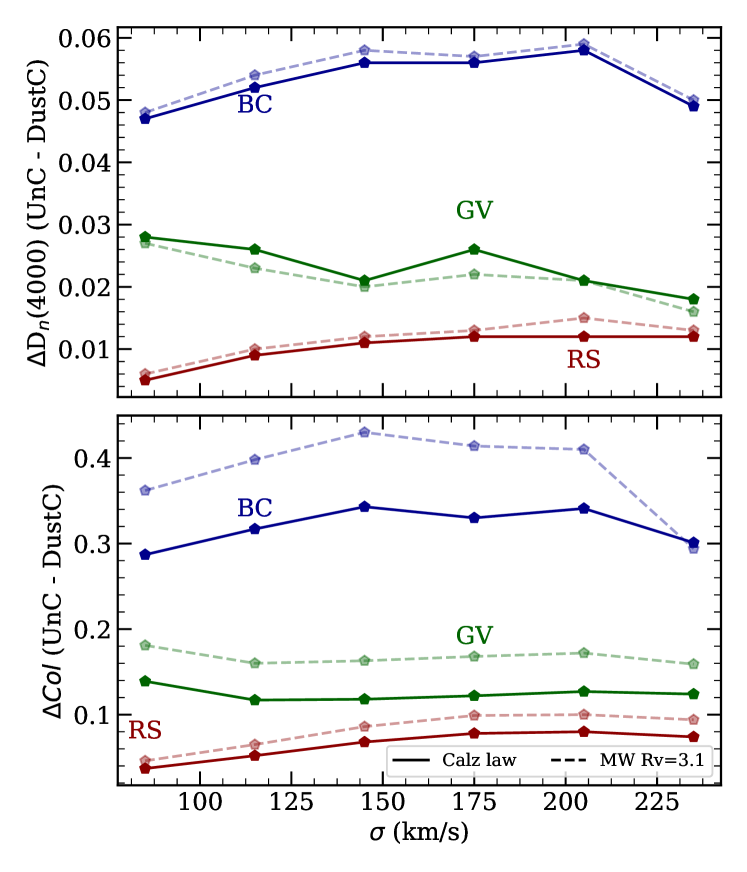
Figure 14: Dependence of 4000Å break strength (top) and ($g-r$) colour (bottom) on dust attenuation. The blue, green and red data points show the difference in 4000Å break strength (top) and colour (bottom), after correction for dust attenuation. The solid and dashed lines represent the two attenuation laws considered, Calzetti et al. (2000) and Cardelli et al. (1989), respectively.

To illustrate the dependence of the 4000Å break and colour-selection of GV galaxies with respect to dust attenuation, we compare in Fig. 14 the difference between the trends found for the location of the BC (blue); GV (green) and RS (red), as a function of velocity dispersion. Each one corresponds to the mean of the PDF associated to each sub-population (see Sec. 2.2). The top and bottom panels display the difference between BC, GV and RS with and without dust correction for D_n(4000) and colour, respectively. To test for systematics we apply either a Milky Way extinction law (Cardelli et al., 1989, dashed lines) or a Calzetti et al. (2000, solid lines) law. Note the small difference when using the selection based on break strength (top panels), especially on GV galaxies, at the level $\Delta D_{n}(4000)<$0.03, whereas the colours (bottom panels) are not only substantially affected – with correction terms comparable to the actual separation between BC and RS, but are also heavily dependent on the attenuation law adopted, and thus prone to systematics from the variance regarding the details of dust composition and geometry.

Appendix C The effect of aperture

This study focuses on the use of spectroscopic data of the classic SDSS dataset, therefore confined to a 3 arcsec diameter fibre. For consistency, our comparison with respect to colour, ${}^{0.1}(g-r)$, is done within the same aperture. This could introduce a bias with respect to stellar mass (or velocity dispersion), as more massive, and generally larger, galaxies would have a lower fraction of the light from their stellar populations inside the fibre. To assess this bias, we use the JHU/MPA catalogue (Kauffmann et al., 2003) and compare the colour within the aperture with the modelled colour for the whole galaxy (Fig. 15). The difference between these two definitions of colour shows a minimal trend with stellar mass. Due to D_n(4000) tracing the average age in a similar manner to colour, we expect a similar, minor, difference between D_n(4000) inside the fibre and D_n(4000) measured in the whole galaxy.

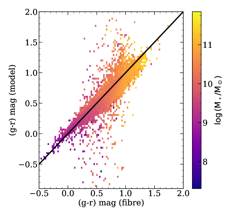
Figure 15: Relation between the colour measured inside the 3 arcsec fibre, and the one from a surface brightness modelling to the whole galaxy (i.e. determined from the official SDSS model magnitudes). The data are colour coded with respect to stellar mass (colour bar on the right). The solid black line illustrates a 1:1 correspondence.

Though there is no bias in relation to stellar mass, we do see an offset between the colour in the fibre and that of the whole galaxy. Therefore, a similar behaviour in D_n(4000) is expected. The inconsistency in colour between fibre and whole galaxy is partially due to biases from surface brightness modelling, as well as from the presence of gradients in population content. One physical mechanism that can give rise to these gradients is the inside-out/outside-in quenching. For instance, inside-out quenching will result in younger populations outside of the reach of the fibre (Kelvin et al., 2018). The opposite will be true when galaxy is undergoing outside-in quenching. Another cause for such behaviour would be galaxy morphology. More specifically, spiral galaxies with a strong bulge will produce a greater difference between fibre and whole galaxy estimates of both the colour and D_n(4000).

Appendix D SDSS Green Valley Probability Catalogue

Adopting the methodology laid out in A19, we are able to assign to each galaxy, on the D_n(4000) vs velocity dispersion plane, a probability of it belonging to the Blue Cloud ($\hat{\cal P}_{BC}$), Green Valley ($\hat{\cal P}_{GV}$), or Red Sequence ($\hat{\cal P}_{RS}$). Each probability can be written:

$$\hat{\cal P}_{k}=\eta_{k}{\cal P}_{k}(\pi;\sigma),$$ (10)

where ${\cal P}_{k}$ is given by Eq. 2 and $\eta_{k}$ is a weight factor dependent on the number of galaxies in BC, GV or RS.

To assign a probability to an individual galaxy, we firstly obtain the PDF averages: $\mu_{BC}$, $\mu_{GV}$, $\mu_{RS}$, and “widths”: $s_{BC}$, $s_{GV}$ and $s_{RS}$ for 11 bins from 50 to 350 km/s. Then we interpolate between the velocity dispersion bins with a third order polynomial that enables us to find the effective $\mu_{k}$ and $s_{k}$ in each group, BC, GV and RS, at any velocity dispersion. For each galaxy, we obtain its ${\cal P}_{k}({\cal G}_{i})$, along with $\mu_{k}({\cal G}_{i})$ and $s_{k}({\cal G}_{i})$. To determine $\eta_{k}$, we select all galaxies with velocity dispersion within an interval centered at the $\sigma$ of the chosen galaxy, with width $\Delta\sigma$=15 km/s, and then assign them either to the BC, GV or RS, following the methodology described in A19, and in Sec. 2.2 of this paper. For any galaxy sitting on adjacent regions, we assign them evenly to their overlapping regions; e.g., if they overlap between BC and GV, they are equally likely to count towards the BC or GV. Thus we obtain $\eta_{k}$ for each galaxy. Once we obtain $\hat{\cal P}_{k}$, we normalise the total probability to unity. Note we assign galaxies with D_n(4000)$>$1.99, $\hat{\cal P}_{RS}$=1, and $\hat{\cal P}_{BC}=\hat{\cal P}_{GV}$=0, as we know that galaxies with a high 4000 Å break strength are old and quiescent. Likewise galaxies with D_n(4000)$<$0.8 are assigned $\hat{\cal P}_{BC}$=1, and $\hat{\cal P}_{GV}=\hat{\cal P}_{RS}$=0.

A small number of galaxies from the catalogue is shown in Tab. 2 for reference. The full catalogue can be found in the online version of the paper. Note owing to the methology used, the probabilites presented here are not unique solutions, but a realisation of the three groups. Thus if one were to carry out the outlined steps, the results should not be identical, but statistically equivalent. Fig. 16 illustrates the probability density of galaxies residing in BC, GV or RS, as presented in A19 and this paper.

Table 2: Probabilities of BC, GV or RS membership assigned to each galaxy from the SDSS set. This table shows a small portion of the full set, giving the SDSS spectral identification (plate, Julian date and fibre ID) along with the 4000Å break strength and velocity dispersion (measured within the 3 arcsec diameter fibres of the spectrograph). The final three columns list the normalized probability of belonging to either Blue Cloud, Green Valley, or Red Sequence, respectively, using the methodology presented here and in A19.

SDSS ID				Velocity	Probabilities
plate	mjd	fibre ID	Dn(4000)	dispersion	$\hat{\cal P}_{BC}$	$\hat{\cal P}_{GV}$	$\hat{\cal P}_{RS}$
				km/s
315	51663	560	1.012	64.5	0.970	0.009	0.021
326	52375	86	1.584	99.2	0.001	0.026	0.973
326	52375	119	1.509	104.6	0.011	0.360	0.629
326	52375	150	1.777	168.2	0.000	0.000	1.000
327	52294	147	1.651	147.9	0.001	0.013	0.986

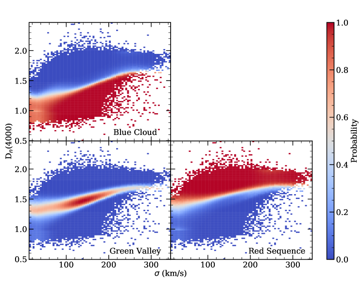
Figure 16: The probability of galaxies belonging to the Blue Cloud (top left), Green Valley (bottom left) and Red Sequence (bottom right). Blue colours represent galaxies with a low probability of residing in the three regions, as labelled, while red shows high probability (see colour bar for reference). For ease of visualisation, the resulting density plots have been modified with a Gaussian smoothing kernel.

References

- Abolfathi et al. (2018) Abolfathi B., et al., 2018, ApJS, 235, 42
- Angthopo et al. (2019) Angthopo J., Ferreras I., Silk J., 2019, MNRAS, 488, L99 (A19)
- Aparicio Villegas et al. (2010) Aparicio Villegas T., et al., 2010, AJ, 139, 1242
- Baldry et al. (2004) Baldry I. K., Glazebrook K., Brinkmann J., Ivezić Ž., Lupton R. H., Nichol R. C., Szalay A. S., 2004, ApJ, 600, 681
- Baldwin et al. (1981) Baldwin J. A., Phillips M. M., Terlevich R., 1981, PASP, 93, 5
- Balogh et al. (1999) Balogh M. L., Morris S. L., Yee H. K. C., Carlberg R. G., Ellingson E., 1999, ApJ, 527, 54
- Bell et al. (2004) Bell E. F., et al., 2004, ApJ, 608, 752
- Benitez et al. (2014) Benitez N., et al., 2014, J-PAS red book, p. arXiv:1403.5237
- Bernardi et al. (2003) Bernardi M., et al., 2003, AJ, 125, 1882
- Bremer et al. (2018) Bremer M. N., et al., 2018, MNRAS, 476, 12
- Brinchmann et al. (2004) Brinchmann J., Charlot S., White S. D. M., Tremonti C., Kauffmann G., Heckman T., Brinkmann J., 2004, MNRAS, 351, 1151
- Bruzual (1983) Bruzual G., 1983, ApJ, 273, 105
- Bruzual & Charlot (2003) Bruzual G., Charlot S., 2003, MNRAS, 344, 1000
- Calzetti et al. (2000) Calzetti D., Armus L., Bohlin R. C., Kinney A. L., Koornneef J., Storchi-Bergmann T., 2000, ApJ, 533, 682
- Cappellari & Emsellem (2004) Cappellari M., Emsellem E., 2004, PASP, 116, 138
- Cardelli et al. (1989) Cardelli J. A., Clayton G. C., Mathis J. S., 1989, ApJ, 345, 245
- Chabrier (2003) Chabrier G., 2003, PASP, 115, 763
- Charlot & Fall (2000) Charlot S., Fall S. M., 2000, ApJ, 539, 718
- Cibinel et al. (2013) Cibinel A., et al., 2013, ApJ, 777, 116
- Cid Fernandes et al. (2005) Cid Fernandes R., Mateus A., Sodré L., Stasińska G., Gomes J. M., 2005, MNRAS, 358, 363
- Coenda et al. (2018) Coenda V., Martínez H. J., Muriel H., 2018, MNRAS, 473, 5617
- Eales et al. (2018) Eales S. A., et al., 2018, MNRAS, 481, 1183
- Faber et al. (2007) Faber S. M., et al., 2007, ApJ, 665, 265
- Fang et al. (2012) Fang J. J., Faber S. M., Salim S., Graves G. J., Rich R. M., 2012, ApJ, 761, 23
- Ferreras et al. (1999) Ferreras I., Charlot S., Silk J., 1999, ApJ, 521, 81
- Ferreras et al. (2009) Ferreras I., et al., 2009, ApJ, 706, 158
- Ferreras et al. (2013) Ferreras I., La Barbera F., de La Rosa I. G., Vazdekis A., de Carvalho R. R., Falcon-Barroso J., Ricciardelli E., 2013, MNRAS, 429, L15
- Ferreras et al. (2019) Ferreras I., et al., 2019, MNRAS, 489, 608
- Gabor et al. (2010) Gabor J. M., Davé R., Finlator K., Oppenheimer B. D., 2010, MNRAS, 407, 749
- Gallazzi et al. (2005) Gallazzi A., Charlot S., Brinchmann J., White S. D. M., Tremonti C. A., 2005, MNRAS, 362, 41
- Galliano et al. (2018) Galliano F., Galametz M., Jones A. P., 2018, ARA&A, 56, 673
- Gonçalves et al. (2012) Gonçalves T. S., Martin D. C., Menéndez-Delmestre K., Wyder T. K., Koekemoer A., 2012, ApJ, 759, 67
- Graves et al. (2009) Graves G. J., Faber S. M., Schiavon R. P., 2009, ApJ, 693, 486
- Graves et al. (2010) Graves G. J., Faber S. M., Schiavon R. P., 2010, ApJ, 721, 278
- Hathi et al. (2009) Hathi N. P., Ferreras I., Pasquali A., Malhotra S., Rhoads J. E., Pirzkal N., Windhorst R. A., Xu C., 2009, ApJ, 690, 1866
- Hernán-Caballero et al. (2013) Hernán-Caballero A., et al., 2013, MNRAS, 434, 2136
- Hogg et al. (2002) Hogg D. W., Baldry I. K., Blanton M. R., Eisenstein D. J., 2002, arXiv e-prints, pp astro–ph/0210394
- Hopkins et al. (2006) Hopkins P. F., Hernquist L., Cox T. J., Di Matteo T., Robertson B., Springel V., 2006, ApJS, 163, 1
- Kauffmann et al. (2003) Kauffmann G., et al., 2003, MNRAS, 341, 33
- Kelvin et al. (2018) Kelvin L. S., et al., 2018, MNRAS, 477, 4116
- Kriek & Conroy (2013) Kriek M., Conroy C., 2013, ApJ, 775, L16
- Kroupa (2001) Kroupa P., 2001, MNRAS, 322, 231
- La Barbera et al. (2013) La Barbera F., Ferreras I., Vazdekis A., de la Rosa I. G., de Carvalho R. R., Trevisan M., Falcón-Barroso J., Ricciardelli E., 2013, MNRAS, 433, 3017
- La Barbera et al. (2014) La Barbera F., Pasquali A., Ferreras I., Gallazzi A., de Carvalho R. R., de la Rosa I. G., 2014, MNRAS, 445, 1977
- Laureijs et al. (2011) Laureijs R., et al., 2011, Euclid red book, p. arXiv:1110.3193
- Martin et al. (2007) Martin D. C., et al., 2007, ApJS, 173, 342
- Matteucci & Recchi (2001) Matteucci F., Recchi S., 2001, ApJ, 558, 351
- Mendez et al. (2011) Mendez A. J., Coil A. L., Lotz J., Salim S., Moustakas J., Simard L., 2011, ApJ, 736, 110
- Narayanan et al. (2018) Narayanan D., Conroy C., Davé R., Johnson B. D., Popping G., 2018, ApJ, 869, 70
- Nelson et al. (2018) Nelson D., et al., 2018, MNRAS, 475, 624
- Nogueira-Cavalcante et al. (2018) Nogueira-Cavalcante J. P., Gonçalves T. S., Menéndez-Delmestre K., Sheth K., 2018, MNRAS, 473, 1346
- Pérez-González et al. (2013) Pérez-González P. G., et al., 2013, ApJ, 762, 46
- Phillipps et al. (2019) Phillipps S., et al., 2019, MNRAS, 485, 5559
- Pirzkal et al. (2017) Pirzkal N., et al., 2017, ApJ, 846, 84
- Poggianti & Barbaro (1997) Poggianti B. M., Barbaro G., 1997, A&A, 325, 1025
- Salim (2014) Salim S., 2014, Serbian Astron. J., 189, 1
- Salim & Rich (2010) Salim S., Rich R. M., 2010, ApJ, 714, L290
- Salim et al. (2018) Salim S., Boquien M., Lee J. C., 2018, ApJ, 859, 11
- Sansom & Northeast (2008) Sansom A. E., Northeast M. S., 2008, MNRAS, 387, 331
- Schawinski et al. (2007) Schawinski K., Thomas D., Sarzi M., Maraston C., Kaviraj S., Joo S.-J., Yi S. K., Silk J., 2007, MNRAS, 382, 1415
- Schawinski et al. (2014) Schawinski K., et al., 2014, MNRAS, 440, 889
- Schiminovich et al. (2007) Schiminovich D., et al., 2007, ApJS, 173, 315
- Smee et al. (2013) Smee S. A., et al., 2013, AJ, 146, 32
- Smethurst et al. (2015) Smethurst R. J., et al., 2015, MNRAS, 450, 435
- Spergel et al. (2015) Spergel D., et al., 2015, WFIRST-AFTA 2015 Report, p. arXiv:1503.03757
- Strateva et al. (2001) Strateva I., et al., 2001, AJ, 122, 1861
- Taylor et al. (2015) Taylor E. N., et al., 2015, MNRAS, 446, 2144
- Thilker et al. (2010) Thilker D. A., et al., 2010, ApJ, 714, L171
- Thomas et al. (1999) Thomas D., Greggio L., Bender R., 1999, MNRAS, 302, 537
- Thomas et al. (2003) Thomas D., Maraston C., Bender R., 2003, MNRAS, 339, 897
- Thomas et al. (2010) Thomas D., Maraston C., Schawinski K., Sarzi M., Silk J., 2010, MNRAS, 404, 1775
- Trager et al. (1998) Trager S. C., Worthey G., Faber S. M., Burstein D., González J. J., 1998, ApJS, 116, 1
- Trayford et al. (2016) Trayford J. W., Theuns T., Bower R. G., Crain R. A., Lagos C. d. P., Schaller M., Schaye J., 2016, MNRAS, 460, 3925
- Tress et al. (2018) Tress M., et al., 2018, MNRAS, 475, 2363
- Vazdekis et al. (2012) Vazdekis A., Ricciardelli E., Cenarro A. J., Rivero-González J. G., Díaz-García L. A., Falcón-Barroso J., 2012, MNRAS, 424, 157
- Wilkinson et al. (2017) Wilkinson D. M., Maraston C., Goddard D., Thomas D., Parikh T., 2017, MNRAS, 472, 4297
- Williams et al. (2009) Williams R. J., Quadri R. F., Franx M., van Dokkum P., Labbé I., 2009, ApJ, 691, 1879
- Worthey (1994) Worthey G., 1994, ApJS, 95, 107
- Worthey & Ottaviani (1997) Worthey G., Ottaviani D. L., 1997, ApJS, 111, 377
- Wright et al. (2019) Wright R. J., Lagos C. d. P., Davies L. J. M., Power C., Trayford J. W., Wong O. I., 2019, MNRAS, 487, 3740
- York et al. (2000) York D. G., et al., 2000, AJ, 120, 1579
- de la Rosa et al. (2011) de la Rosa I. G., La Barbera F., Ferreras I., de Carvalho R. R., 2011, MNRAS, 418, L74